Differential rotation in K, G, F and A stars

Abstract

Rotational light modulation in Kepler photometry of K – A stars is used to estimate the absolute rotational shear. The rotation frequency spread in 2562 carefully selected stars with known rotation periods is measured using time-frequency diagrams. The variation of rotational shear as a function of effective temperature in restricted ranges of rotation period is determined. The shear increases to a maximum in F stars, but decreases somewhat in the A stars. Theoretical models reproduce the temperature variation quite well. The dependence of rotation shear on rotation rate in restricted temperature ranges is also determined. The dependence of the shear on the rotation rate is weak in K and G stars, increases rapidly for F stars and is strongest in A stars. For stars earlier than type K, a discrepancy exists between the predicted and observed variation of shear with rotation rate. There is a strong increase in the fraction of stars with zero frequency spread with increasing effective temperature. The time-frequency diagrams for A stars are no different from those in cool stars, further supporting the presence of spots in stars with radiative envelopes.

1 Introduction

The rotation period of an individual sunspot depends on it latitude: the higher the latitude, the longer the period. Examination of spectral line Doppler shifts at the limb of the Sun shows that the rotational velocity has the same latitude dependence as sunspot rotation rates. In addition, helioseismic measurements have revealed the internal rotation profile of the Sun. This shows that differential rotation varies with depth as well as latitude. However, the radiative inner core of the Sun appears to rotate almost as a solid body (Thompson et al., 2003).

Most cool stars, either fully convective or with a convective envelope like the Sun, will have spots on their surfaces, giving rise to light variations. The rotation periods can be obtained from a time series of photometric observations. Over 500 stars of spectral types F–M observed from the ground are classified as rotational variables (Strassmeier, 2009). The Kepler mission has been a very fruitful source for the study of starspots and the rotation periods of many thousands of cool Kepler stars have been measured (McQuillan et al., 2013, 2014; Reinhold et al., 2013; Nielsen et al., 2013).

Surface differential rotation can be inferred using three different techniques. The first technique is Doppler imaging (DI). In DI the location of individual spots can be estimated from their effect on the spectral line profiles, provided the star is rotating at a sufficiently high rate (Collier Cameron et al., 2002). A time series of Doppler images obtained with high dispersion and high signal to noise (S/N) allows differential rotation to be measured from differences in the rotation periods of individual spots at different latitudes. The second technique is the Fourier transform (FT) method (Reiners & Schmitt, 2002). In the FT method, the Doppler shift at different latitudes due to rotation can be inferred from the Fourier transform of the line profiles. Note that the star does not need have starspots for this method to be used, but a spectrum with very high S/N is required. The method is limited to stars with moderate and rapid rotation. The big advantage is that latitudinal differential rotation can be measured from a single exposure. The third method, time series photometry, has already been mentioned. By following the variation of rotation period over time, a lower limit can be estimated for the rotational shear. If there is more than one starspot at different latitudes, photometric measurements will show close multiple periods. The range in periods provides a lower limit to the rotational shear (Reinhold et al., 2013).

The latitudinal differential rotation in stars is usually described by a law of the form $\Omega(\theta)=\Omega_{e}(1-\alpha\sin^{2}\theta)$, where $\theta$ is the latitude and $\Omega_{e}$ the angular rotation rate at the equator. The rotational shear is the difference in rotation rate between the equator and pole, $\Delta\Omega=\Omega_{e}-\Omega_{p}=\alpha\Omega_{e}$. For the Sun $\alpha=0.2$. Differential rotation is categorized as “solar-like” when $\alpha>0$, or as “antisolar” when the polar regions rotate faster than the equator ($\alpha<0$). In order to determine $\alpha$, the latitude of a spot needs to be known. This can only be done with the DI method. Photometric methods can only provide a lower limit of $\Delta\Omega$. It is difficult to determine the sign of $\alpha$ and usually only the absolute value can be inferred.

Investigation of differential rotation in stars has a long history. Henry et al. (1995) monitored the light curves of four active binary stars and found that their rotation periods changed with time, suggesting differential rotation. From photometric time series observations of 36 cool stars, Donahue et al. (1996) found that the range of period variation increases with increasing period. Reiners & Schmitt (2003) used the FT method to estimate $\alpha$ in 32 stars of spectral types F0–G0. Non-zero values of $\alpha$ were obtained for 10 stars. They find that differential rotation appears to be more common in slower rotators and that the rotational shear depends on the rotation period.

Barnes et al. (2005a) applied the DI technique to 10 G2–M2 stars and found that rotational shear increases with effective temperature. They find a weak dependence on rotation rate. Using the FT method, Reiners (2006) concluded that A stars generally rotate as solid bodies. Using the same method, Ammler-von Eiff & Reiners (2012) were able to measure differential rotation in 33 A–F stars. They found evidence for two populations of differential rotators: one of rapidly rotating late A stars at the granulation boundary with strong horizontal shear and the other of mid- to late-F type stars with moderate rates of rotation and less shear.

The photometric method in which a periodogram is used to detect multiple close rotation periods has been used by Reinhold et al. (2013) for Kepler stars with $T_{\rm eff}<6000$ K. They find that $\alpha$ increases with rotational period, and slightly increases towards cooler stars. The absolute shear shows only a weak dependence on rotation period over a large period range. More recently, Reinhold & Gizon (2015) confirmed that $\alpha$ increases with rotation period for stars with $T_{\rm eff}<6700$ K, while hotter stars show the opposite behaviour.

In summary, there is general agreement that the rotational shear, $\Delta\Omega$, is low in M and K stars and reaches a maximum in F stars. The dependence of shear with period seems to be weak. The DI and FT methods require expensive resources and cannot be applied to stars with slow rotation. Kepler photometry provides an invaluable resource, consisting of nearly four years of almost uninterrupted photometric measurements with unprecedented precision at a cadence of 30 min. While progress has been made in investigating differential rotation in these stars (Reinhold et al., 2013; Reinhold & Gizon, 2015), the results are somewhat confusing.

In this paper we selected a sample of Kepler stars with known rotation periods, but excluded pulsating stars and eclipsing variables. A different approach is used to estimate the rotational shear. Instead of relying on a secondary period, we construct a time-frequency diagram for each star. In this way, spots with variable frequencies and amplitudes can be recognized by visual inspection of the time-frequency diagram presented as a grayscale image. The total spread in rotation frequency for each star is estimated, giving a lower bound for $\Delta\Omega$. In addition, the analysis is extended to A stars which in the past have been neglected in the belief that starspots should not exist in stars with radiative envelopes.

2 The data

Kepler light curves are available as uncorrected simple aperture photometry (SAP) and with pre-search data conditioning (PDC) in which instrumental effects are removed (Stumpe et al., 2012; Smith et al., 2012). The vast majority of the stars are observed in long-cadence (LC) mode with exposure times of about 30 min. These data are publicly available on the Barbara A. Mikulski Archive for Space Telescopes (MAST, archive.stsci.edu). We used all available PDC data for each star.

The sample is taken from a list of over 20000 Kepler stars which consists of all stars observed in long-cadence mode (30 min cadence) and $T_{\rm eff}>6500$ K and nearly all stars with Kepler magnitude $K_{p}<12.5$ mag. We classified these stars according to variability type. Most of the stars with $6500<T_{\rm eff}<7500$ K could not be used because they have multiple stable frequencies and amplitudes. These are the pulsating $\gamma$ Doradus variables. The $\delta$ Scuti stars, which are the only other type of pulsating main sequence star later than type B, are easily identified by the presence of high frequencies. These were excluded as were eclipsing binaries.

Of the remaining stars, only those appearing in the catalogues of rotation periods by (McQuillan et al., 2014) or Reinhold et al. (2013) (stars cooler than 7500 K) or Balona (2013) (A-type stars) were selected. The stars are all on the main sequence with rotation periods shorter than about 30 d.

3 Method

Because we expect starspots to migrate in latitude, the rotation frequency may slightly change with time. This results in a broadening of the rotational peak in the periodogram of the whole data set. If the spot changes size or contrast, the resulting change in light amplitude will also cause line broadening. These effects tend to reduce the visibility of a spot in the periodogram and the estimated frequency spread will be reduced. To avoid this problem, we need to sample the frequency and amplitude of the spot over a sufficiently small time interval. The evolution of frequency and amplitude with time can be constructed by sampling the periodogram over a limited time span at regular intervals over the whole light curve. The time span used for the periodogram is called the “window size”.

The choice of window size requires some consideration. If it is small, time resolution is good, but frequency resolution is poor and vice-versa. After some trial and error, we settled on a window size of 200 d and a step size of 20 d. In calculating the time-frequency diagram we used a weighting scheme in which points further from a given time step are given lower weights in accordance with a Gaussian. We chose the FWHM of the Gaussian to be half the window size (i.e. FWHM = 100 d). However, the result does not depend very much on the FWHM or even if the points are given the same weight. The window size of the first and last sampling times are, of necessity, only half the chosen window size. It is possible to use the full window size only after the first 100 d and before the last 100 d in the data set. The Lomb-Scargle periodogram for unequally-spaced data (Press & Rybicki, 1989) was used in constructing the time-frequency diagram.

The time-frequency diagram can be displayed as a grayscale image in which a sinusoidal signal of constant period and amplitude appears as a sharp line of constant intensity. A spot which drifts in latitude and changes in size or contrast will appear as a curve with variable intensity. The time-frequency diagram thus displays how the spot evolves in period and amplitude and can be used to discriminate between a starspot and a pulsational signal, for example. Furthermore, spots which might exist for a short period, and which would not necessarily give rise to a significant secondary peak in the periodogram, will be easier to detect.

Examples of time-frequency grayscale plots are shown in Fig. 1. As the figure shows, the grayscale image does not show just a single line, but a band of closely-spaced and often interweaving lines of variable intensity caused by spots drifting in latitude and of finite lifetime. A lower limit of the rotation shear, $\Delta\Omega$, is obtained from the frequency difference between the highest and lowest frequencies. The shear can be measured in 2562 stars. For most of these stars, the first harmonic of the rotation frequency is also visible.

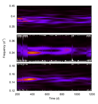
Figure 1: Examples of time-frequency grayscale plots. The top panel is for KIC 7135294 ($T_{\rm eff}=5953$ K), the middle panel KIC 12061741 ($T_{\rm eff}=9169$ K) and the bottom panel KIC 3122749 ($T_{\rm eff}=9745$ K).

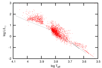
Figure 2: The H-R diagram for stars with measured values of the differential rotation shear. The dashed line is the solar abundance zero-age main sequence from Bertelli et al. (2008).

4 Normalization

The frequency spread, $\delta\omega$ estimated from the time-frequency plots provides only a lower bound for the shear, $\Delta\Omega$. For two spots at latitudes $\theta_{1}$ and $\theta_{2}$, $\delta\omega=\Delta\Omega(|\sin^{2}\theta_{2}-\sin^{2}\theta_{1}|)=f\Delta\Omega$. The unknown factor $f$ depends on the spot locations. Hall & Henry (1994) made a simple estimate of $f$ on the assumption that spots are equally spaced in latitude, in which case $f$ is easily calculated as a function of the number of spots. It turns out that $0.5<f<1.0$.

In general, we do not know the number of spots or their distribution in latitude unless the DI method is used. Usually, discussions in the literature are confined to the power laws describing how $\Delta\Omega$ varies with effective temperature or rotation rate, which do not require knowledge of the scaling factor, $f$. An alternative approach is to assume that $\Delta\Omega$ in stars with approximately the same effective temperature and rotation period as the Sun will be the solar value, $\Delta\Omega_{\odot}=0.073$ rad d^-1. The normalization procedure consists in finding the mean of the frequency spread, $\langle\delta\omega\rangle$, for a group of stars with similar effective temperatures and rotation periods as the Sun and using $f=\langle\delta\omega\rangle/\Delta\Omega_{\odot}$.

To obtain the normalizing factor, we selected stars with $5300<T_{\rm eff}<6300$ K and $20<P_{\rm rot}<30$ d from which we obtain $\langle\delta\omega\rangle=0.104\pm 0.005$ rad d^-1 and $f=1.43\pm 0.06$ from 82 stars. The fact that $f>1$ is a surprise. Perhaps the assumption that rotational shear in these stars is similar to that in the Sun is not correct.

5 Results

In Fig. 2 we show the location of the stars in the H-R diagram. Effective temperatures, surface gravities and metallicities were taken from Huber et al. (2014). The luminosities are calculated using the relationships in Torres et al. (2010). The pulsating $\gamma$ Dor stars have multiple frequencies within the range of the expected rotational frequencies. It is not possible to distinguish between rotational modulation and pulsation in these stars, so they were excluded. A large fraction of F stars appear to be $\gamma$ Dor variables, which accounts for the gap in the 6500–7500 K range in Fig. 2.

The A stars are usually omitted in discussions of starspots. This follows from the long-held view that radiative atmospheres cannot support a magnetic field; hence no starspots should exist. However, even a quick inspection of the Kepler A-star light curves shows that this view is not correct, as discussed in Balona (2013). In fact, the time-frequency diagrams for A stars do not differ in any general way from those of F, G, or K stars. Fig. 1 includes the time-frequency diagrams for two early A stars.

The properties of the sample of stars used in this investigation are shown in Table 1. The number of stars with a measurable frequency spread is given by $N$. In some cases no frequency spread could be measured, and $\Delta\Omega=0$. The number of these stars is given by $N_{0}$. The mean values of the normalized shear and $\alpha$ are also shown.

Table 1: The number of stars, $N$, within the given effective temperature range, and with $\Delta\Omega>0$ is given. $N_{0}$ is the number of stars with $\Delta\Omega=0$. The mean rotation period, $P_{\rm rot}$, the mean rotational shear, $\Delta\Omega$, and the mean relative shear, $\alpha$ are shown. Values of $\Delta\Omega$ have been normalized to the Sun.

Sp.Ty.	$T_{\rm eff}$	$N$	$N_{0}$	$P_{\rm rot}$	$\Delta\Omega$	$\alpha$
	K			d	rad d-1
K9–G9	3600–5000	166	4	11.90	0.039	0.072
K3–G4	4500–5600	272	4	12.09	0.068	0.126
G7–G1	5200–5900	385	8	12.42	0.083	0.157
G4–F8	5600–6200	604	20	11.08	0.112	0.181
G0–F6	6000–6600	969	82	8.27	0.159	0.172
F0–A0	7400–10000	315	207	3.41	0.263	0.066

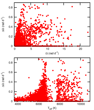
Figure 3: Individual measurements of normalized differential rotation shear, $\Delta\Omega$, as a function of angular rotation rate (top panel) and effective temperature (bottom panel).

6 Variation of the shear with effective temperature and rotation

Fig. 3 shows the normalized estimates of $\Delta\Omega$ as a function of effective temperature and rotation rate for each star. $\Delta\Omega$ increases with effective temperature up to the convective boundary, but decreases slightly for the A stars. In general the shear increases with increasing rotation rate.

It is evident that the shear is a complex function of both effective temperature and rotation rate. Since only a lower bound of $\Delta\Omega$ is measured, a relatively large number of stars within a given range of effective temperature and rotation rate is required to minimize uncertainties. Because of the small number of stars, previous attempts have used stars of all rotation rates to analyse the dependence of the shear on effective temperature. In the same way, stars of all effective temperatures have been used to determine the dependence of shear on the rotation rate. This has prevented any meaningful estimate on how $\Delta\Omega$ varies independently with effective temperature and rotation rate. The sample of 2562 Kepler stars is sufficiently large to solve this problem.

The relationship between the shear and effective temperature needs to be evaluated for constant values of rotation rate, $\Omega$. For this purpose the mean rotation frequency spread of stars within a small range of $\Omega$ was calculated. Stars with zero frequency spread were not included. Fig. 4 shows how $\Delta\Omega$ in stars with approximately the same rotational period varies with effective temperature.

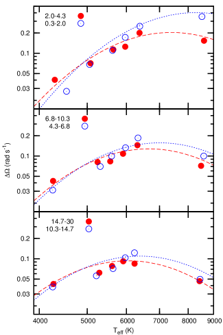
Figure 4: The normalized differential rotation shear, $\Delta\Omega$, as a function of effective temperature for the indicated ranges of rotation period (in days). The curves are calculated using the interpolation formula Eq. 1.

In the same way, to evaluate the relationship between the shear and rotation rate, the mean rotation frequency spread of stars within a small range of effective temperature was calculated. Fig. 5 shows how $\Delta\Omega$ in stars of about the same effective temperature varies with rotation rate.

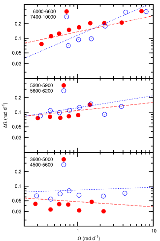
Figure 5: The variation of $\Delta\Omega$ as a function of angular rotation frequency for the indicated ranges of effective temperature. The solid curves are calculated using the interpolation formula.

The figures show that $\Delta\Omega$ is weakly dependent on effective temperature for slowly rotating stars, but the dependence increases with increasing rotation rate. For K and G stars there is very little dependence of $\Delta\Omega$ on rotation rate, but this dependence increases for F and A stars. The fact that the shear depends on effective temperature and rotation rate in a rather complex way probably explains why there is so much disagreement in the literature.

A reasonable fit to the data may be obtained using the following interpolation formula:

$$\log\Delta\Omega =-211.12+109.67x-11.14y-14.30x^{2}+3.02xy,$$ (1)

where $x=\log T_{\rm eff}$ and $y=\log\Omega$ with $\Omega$ and $\Delta\Omega$ in rad d^-1. In Figs. 4 and 5, the curves show $\Delta\Omega$ calculated from this formula.

7 Comparison with previous observations

Several observational studies have found a power law of the form $\Delta\Omega\propto\Omega^{n}$. By measuring the change in rotation periods in 36 F–K stars, Donahue et al. (1996) found that $n\approx 0.7$. Messina & Guinan (2003) estimated $n\approx 0.6$ from the period variation in 14 K5–G2 stars. Barnes et al. (2005a) find $n\approx 0.15$ by combining their DI results of 10 stars with previous studies. Using the FT method, Reiners (2006) find $n\approx 1.5$ from 10 F and G stars. Using the interpolation formula we get $n=-0.1$, 0.2, 0.4 and 0.7 for K, G, F and A stars respectively. It is evident that the relationship depends rather sensitively on the effective temperature.

There is also a power law relating $\Delta\Omega$ to effective temperature of the form $\Delta\Omega\propto T_{\rm eff}^{p}$. Barnes et al. (2005a) found $p\approx 8.9$. The interpolation formula gives $p=6.4$, 3.5, 1.0 and -2.0 for K, G, F and A stars. It is clearly necessary to disentangle the temperature and rotation rate variation for a proper description of the shear.

Table 2: Measurements of rotational shear, $\Delta\Omega$, obtained by Doppler imaging. The star name and effective temperature are given. References are as follows: 1 - Marsden et al. (2004); 2 - Marsden et al. (2005); 3 - Donati et al. (2000); 4 - Barnes et al. (2000); 5 - Collier Cameron & Donati (2002); 6 - Donati et al. (2003); 7 - Barnes et al. (2005a); 8 - Barnes et al. (2005b); 9 - Barnes et al. (2004); 10 - Jeffers & Donati (2009); 11 - Jeffers & Donati (2008); 12 - Järvinen et al. (2015); 13 - Kővári et al. (2014); 14 - Fares et al. (2012); 15 - Kővári et al. (2011); 16 - Waite et al. (2011); 17 - Marsden et al. (2011b); 18 - Marsden et al. (2011a); 19 - Dunstone et al. (2008).

Star	$T_{\rm eff}$	$\Delta\Omega$	$P_{\rm rot}$	Ref.
	K	rad d-1	d
HD 307938	5859	$0.025\pm 0.015$	0.57	1
HD 307938	5859	$0.140\pm 0.010$	0.57	2
LQ Lup	5729	$0.130\pm 0.020$	0.31	3
PZ Tel	5448	$0.101\pm 0.007$	0.95	4
AB Dor	5386	$0.046\pm 0.006$	0.51	5
AB Dor	5386	$0.091\pm 0.012$	0.51	5
AB Dor	5386	$0.089\pm 0.008$	0.51	5
AB Dor	5386	$0.067\pm 0.020$	0.51	5
AB Dor	5386	$0.071\pm 0.006$	0.51	5
AB Dor	5386	$0.058\pm 0.005$	0.51	5
AB Dor	5386	$0.053\pm 0.003$	0.51	6
AB Dor	5386	$0.047\pm 0.003$	0.51	6
AB Dor	5386	$0.058\pm 0.002$	0.51	6
AB Dor	5386	$0.046\pm 0.003$	0.51	6
AB Dor	5386	$0.054\pm 0.001$	0.51	6
HD 197890	4989	$0.032\pm 0.002$	0.38	7
LQ Hya	5019	$0.194\pm 0.022$	1.60	6
LQ Hya	5019	$0.014\pm 0.003$	1.60	6
LO Peg	4577	$0.036\pm 0.007$	0.42	8
HK Aqr	3697	$0.005\pm 0.009$	0.43	9
EY Dra	3489	$0.000\pm 0.003$	0.46	7
HD 171488	5800	$0.340\pm 0.040$	1.33	10
HD 171488	5800	$0.402\pm 0.044$	1.33	10
HD 171488	5800	$0.470\pm 0.044$	1.33	11
AF Lep	6100	$0.259\pm 0.019$	0.97	12
IL HYa	4500	$0.035\pm 0.003$	12.73	13
HD 179949	6160	$0.216\pm 0.061$	7.62	14
V889 Her	5750	$0.042$	1.34	15
HD 106506	5900	$0.240\pm 0.030$	1.39	16
HD 106506	5900	$0.210\pm 0.030$	1.39	16
HD 141943	5850	$0.240\pm 0.030$	2.17	17
HD 141943	5850	$0.360\pm 0.090$	2.17	18
HD 141943	5850	$0.450\pm 0.080$	2.17	18
HD 155555A	5400	$0.078\pm 0.006$	1.67	19
HD 155555A	5400	$0.143\pm 0.008$	1.67	19
HD 155555A	5400	$0.104$	1.67	19
HD 155555B	5050	$0.039\pm 0.006$	1.67	19
HD 155555B	5050	$0.088\pm 0.006$	1.67	19
HD 155555B	5050	$0.060$	1.67	19

The DI technique provides a direct method to estimate $\Delta\Omega$. Table 2, which is an update of Table 1 of Barnes et al. (2005a), lists stars for which $\Delta\Omega$ has been determined. It is interesting to compare these values with the values predicted from Eq. 1. It turns out that the average difference in shear between the stars observed by the DI method and that calculated from the interpolating formula is $\langle\Delta\Omega_{\rm DI}-\Delta\Omega_{\rm Eq1}\rangle=0.000\pm 0.018$ rad d^-1. In other words, there is no significant difference between the two values of $\Delta\Omega$. Also, there is no discernible systematic trend in this difference as a function of effective temperature or rotation period. This suggests that the adopted normalizing factor, $f$, is probably correct. It also suggests that differential rotation in these heavily-spotted stars is similar to that in the Sun.

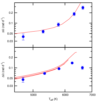
Figure 6: Top panel: the solid line is the variation of $\Delta\Omega$ with effective temperature for models with a rotation period of $P_{\rm rot}=2.5$ d by Küker & Rüdiger (2011). The points are the observed values for stars with $2.0<P_{\rm rot}<3.0$ d. Bottom panel: The lines are models with abundances of $Z=0.01,0.02$ and 0.03 and a rotation period of 10 d by Kitchatinov & Olemskoy (2012). The points are the observed values with $6.0<P_{\rm rot}<14.0$ d. Error bars are one standard deviation in length.

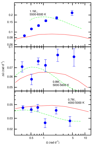
Figure 7: The solid lines are the variation of $\Delta\Omega$ with angular rotation rate for models of stars by Küker & Rüdiger (2011) with the indicated masses. The dashed lines are the corresponding models by Kitchatinov & Olemskoy (2012). The filled circles are normalized values of $\Delta\Omega$ for stars in the indicated range of effective temperature. Error bars are one standard deviation in length.

8 Comparison with theory

Rotation reduces the effective gravity at the equator which, in turn, leads to a temperature variation from equator to pole. This creates a thermal imbalance which is the cause of meridional circulation. Angular momentum transport by convection and by the meridional flow together with the Coriolis force produces differential rotation. Differential rotation of main-sequence dwarfs is predicted to vary mildly with rotation rate but to increase strongly with effective temperature. Meridional circulation and differential rotation are key ingredients in the current theory of the solar dynamo (Choudhuri et al., 1995; Küker & Stix, 2001).

Models of stellar differential rotation for F, G, K and M dwarfs were computed by Küker & Rüdiger (2005) by solving the equation of motion and the equation of convective heat transport in a mean-field formulation. For each spectral type, the rotation rate is varied to study the dependence of the surface shear on this parameter. The horizontal shear, $\Delta\Omega$, turns out to depend strongly on the effective temperature and only weakly on the rotation rate. Later, Küker & Rüdiger (2007) calculated differential rotation specifically for F stars. These models show signs of very strong differential rotation in some cases. Stars just cooler than the granulation boundary have shallow convection zones with short convective turnover times. This leads to a horizontal shear that is much larger than on the solar surface, in agreement with observations.

More recently, Küker & Rüdiger (2011) have further explored the variation of surface differential rotation and meridional flow along the lower part of the zero age main sequence. They construct mean field models of the outer convection zones and compute differential rotation and meridional flow by solving the Reynolds equation with transport coefficients from the second order correlation approximation. For a fixed rotation period of 2.5 d, they find a strong dependence of $\Delta\Omega$ on the effective temperature, which is weak in M dwarfs and rises sharply for F stars (top panel of Fig. 6). The increase with effective temperature is modest below 6000 K but very steep above 6000 K. Both the surface rotation and the meridional circulation are solar-type over the entire temperature range.

They also study the dependence of $\Delta\Omega$ on the rotation rate. This dependence is weak (Fig. 7). Numerical experiments show that for effective temperatures below 6000 K the Reynolds stress is the dominant driver of differential rotation. At this time, there has been no numerical study of differential rotation for A stars.

In Fig. 6 we show how $\Delta\Omega$ varies with $T_{\rm eff}$ for stars with rotation periods in the range 2.0–3.0 d. There is good agreement with the models of Küker & Rüdiger (2011). Fig. 7 shows how $\Delta\Omega$ varies with rotation rate for Kepler stars within limited effective temperature ranges. There agreement with the Küker & Rüdiger (2011) models is reasonable for K stars but there are significant departures for G stars. For F stars the observations depart quite strongly from the models, particularly at high rotation rates. In the models $\Delta\Omega$ attains a maximum at about $\Omega\approx 2$ rad d^-1, whereas the observations show that it increases monotonically with increasing rotation rate.

Kitchatinov & Olemskoy (2012) have also calculated models of differentially rotating stars using the mean field formulation. They find that the dependence of $\Delta\Omega$ on metallicity for stars of a given mass is quite pronounced. However, the dependence almost disappears when differential rotation is considered as a function of effective temperature. Their models of $\Delta\Omega$ as a function of effective temperature for a fixed rotation period of 10 d is compared with observations in the bottom panel of Fig. 6. The agreement is good except for the very hottest stars. Kitchatinov & Olemskoy (2012) also computed models of how $\Delta\Omega$ varies with rotation rate for models with different masses and metallicity $Z=0.02$. The results are shown in Fig. 7. As with Küker & Rüdiger (2011), there is poor agreement with observations except for the K stars.

Augustson et al. (2012) use a three-dimensional anelastic spherical harmonic code to simulate global-scale turbulent flows in 1.2 and $1.3M_{\odot}$ F-type stars at varying rotation rates. They find that differential rotation becomes much stronger with more rapid rotation and larger mass, such that the rotational shear between the equator and a latitude of $60^{\circ}$ is $\Delta\Omega_{60}=0.083\left(\frac{M}{M_{\odot}}\right)^{3.9}\left(\frac{\Omega}{\Omega_{\odot}}\right)^{0.6}$ rad d^-1. The model roughly corresponds to a main sequence star with $T_{\rm eff}\approx 6500$ K.

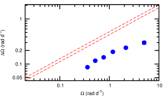
Figure 8: The dashed lines are the $\Delta\Omega_{60}$ relationships of Augustson et al. (2012) for $M/M_{\odot}=1.2$ (bottom line) and 1.3 (top line). The filled circles are the observed values for $6000<T_{\rm eff}<7000$.

In Fig. 8 we show a comparison of this relationship with observations. The slope is in good agreement, though the constant factor is too large for the models.

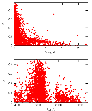
Figure 9: Individual measurements of the relative differential rotation shear, $\alpha$, as a function of effective temperature (bottom panel) and angular rotational rate (top panel).

In summary, it appears that all current models describe the variation of $\Delta\Omega$ with effective temperature rather well. Although models using the mean field formulation seem to describe the variation of $\Delta\Omega$ with rotation rate quite well for K stars, problems begin with the G stars and are very severe in the F stars. The models of Augustson et al. (2012) for F stars gives the correct power law for $\Delta\Omega$ as a function of rotation rate, but the shear is consistently too high.

9 The relative shear, $\alpha$

The relative shear is given by $\alpha=\Delta\Omega/\Omega_{e}$. For each star in our sample we use the normalized value of $\Delta\Omega$ and the known rotation period to obtain $\alpha$. Fig. 9 shows individual values of $\alpha$ as a function of effective temperature and rotation rate.

As before, the mean value of $\alpha$ within narrow ranges of rotation period are calculated as a function of effective temperature. Fig. 10 shows the results. In the same way, the mean value of $\alpha$ within narrow temperature ranges are calculated as a function of rotation rate. This is shown in Fig. 11.

A suitable interpolation formula is given by:

$$\log\alpha =-210.91+109.59x-12.22y-14.30x^{2}+3.05xy,$$ (2)

where $x=\log T_{\rm eff}$ and $y=\log\Omega$ with $\Omega$ and $\Delta\Omega$ in rad d^-1. The fit to the observations are shown in Figs. 10 and 11 by the lines.

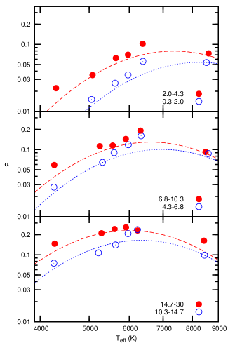
Figure 10: The normalized relative rotational shear, $\alpha$, as a function of effective temperature for the indicated ranges of rotation period (in days). The curves are calculated using the interpolation formula.

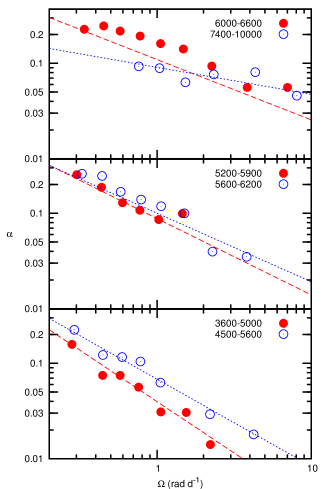
Figure 11: The variation of $\alpha$ as a function of angular rotation frequency for the indicated ranges of effective temperature. The curves are calculated using the interpolation formula.

Notice that the maximum value of $\alpha$ is less than 0.3 for all stars and decreases quite sharply with increasing rotation rate. This is in contrast to the absolute shear which stays the same or increases with rotation rate. The reason for the different behaviour is the rapid increase of rotation rate, $\Omega_{e}$, with effective temperature. For example, the typical rotation period of A stars is about 3 d, while it is around 10 d for K and G stars.

10 The A stars

Because of the perception that starspots cannot exist on stars with radiative envelopes, the A and B stars have been omitted from differential rotation studies using the DI and photometric techniques. The FT method, which measures the shape of the line profile, does not require the presence of starspots. Using this method, Reiners & Royer (2004) and Reiners (2006) were able to detect differential rotation in three mid- to late-A stars. Using the same method, Ammler-von Eiff & Reiners (2012) confirmed differential rotation among the same three A stars near the granulation boundary, but not in other A stars. In fact, no differential rotation was found in stars with $T_{\rm eff}>7400$ K. This is in contrast to our results which clearly show differential rotation in more than half of the Kepler A stars.

It should be noted that the FT method measures $\alpha$, the dimensionless differential rotation constant and not the absolute shear, $\Delta\Omega$. We have seen that the value of $\alpha$ is small for the A stars; in fact $\alpha<0.1$ for nearly all A stars. Ammler-von Eiff & Reiners (2012) state that the detection limit for $\alpha$ is $\approx 0.05$. This means that most of the A stars that were observed by them are probably close to the detection limit for differential rotation. This may be the reason for their failure to detect differential rotation for stars hotter than 7400 K.

In Fig. 12 the average rotational light modulation amplitudes are shown as a function of effective temperature. The amplitudes are large in the K and G stars, but fall sharply for the F and A stars. Let us suppose that the temperature difference between the spot and surrounding photosphere, $\Delta T$, is a constant for stars of all spectral types. It then follows that the light amplitude, which is approximately proportional to $(\Delta T/T)^{4}$, must decrease with increasing temperature, $T$. This contrast effect is most likely responsible for the light amplitude decrease from G to A stars. The rotational light amplitudes for A stars are less than 1 millimag and not detectable from ground-based observations. This is possibly why rotational modulation in A stars escaped detection until recently.

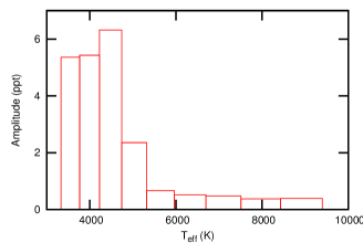
Figure 12: The distribution of rotational modulation amplitude (in parts per thousand) as a function of effective temperature.

The large fraction of A stars with no detectable rotational frequency spread, i.e. with $\Delta\Omega=0$ (see Table 1) deserves attention. In Fig. 13 the relative number of stars with $\Delta\Omega=0$ is shown as a function of effective temperature. It is evident that the numbers of A stars with zero frequency spread is large. In fact, about 40 per cent of A stars showing rotational modulation do not have measurable frequency spread. This fraction decreases sharply for the F stars (about 25 per cent) and is less than 5 per cent for cooler stars.

There is no tendency for stars with zero frequency spread to have significantly different light modulation amplitudes or different rotation rates. There appears to be two distinct groups among the A and F stars: the majority with large differential rotation shear and a smaller group with no shear at all or spots confined to a narrow range of latitude. It would be important to use the FT method with more precision to decide which of the two explanations is correct.

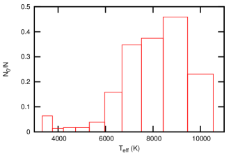
Figure 13: The fraction of stars with $\Delta\Omega=0$ as a function of effective temperature.

11 Summary and discussion

We used Kepler photometry of stars with rotational modulation to measure the frequency spread, $\delta\omega$, around the rotational period. The frequency spread, which is assumed to be a result of starspots at different latitudes, provides a lower bound to the absolute rotational shear, $\Delta\Omega$. Estimation of frequency spread was made by visual examination of time-frequency grayscale diagrams. We were careful to avoid pulsating stars, eclipsing binaries or other types of variable which might be mistaken for rotational modulation. We also confined the sample to stars with known rotational periods. In this way we obtained estimates of $\delta\omega$ for 2562 Kepler stars, including A stars.

The frequency spread is related to the rotational shear by $\delta\omega=f\Delta\Omega$. If it is assumed that the distribution of spots in latitude is approximately the same in all stars, then the average value of $f$ is independent of surface temperature or rotation period. Since $\delta\omega$ provides a lower bound to $\Delta\Omega$, we expect $f<1$. Furthermore, if we assume that surface differential rotation in the Sun is typical of stars with about the same effective temperature and rotation period, then we can obtain $f$ from the mean value of $\delta\omega$ of these stars and the solar value of $\Delta\Omega$. It is found that $f=1.43$, which is puzzling because the frequency spread should be lower than the rotational shear. We suspect that one of the assumptions is not correct. It is possible that $\Delta\Omega$ may be systematically larger in these stars which have spots that are at least 100 times larger than in the Sun.

To investigate the functional dependence of $\Delta\Omega$ on effective temperature we determined $\Delta\Omega$ in restricted ranges of rotation period. In like manner, we found the functional dependence of the shear on the rotation period by determining $\Delta\Omega$ in restricted ranges of effective temperature. The result can be expressed by the interpolation formula, Eq. 1. It is possible that not all stars obey this relationship exactly, since $\Delta\Omega$ probably depends on the history of the star. Eq. 1 should be taken as an approximation which applies, on average, to a group of stars with similar effective temperatures and rotation periods.

The discrepancies which arise in the literature regarding the power law dependence of $\Delta\Omega$ on effective temperature and rotation rate are most likely a result of an insufficient number of stars with known values of rotational shear. We compared $\Delta\Omega$ obtained with the Doppler imaging technique with Eq. 1. There is no significant difference between the two values of $\Delta\Omega$, which provides confidence in the procedure of using the solar value to obtain the normalizing factor, $f$.

We compared the observed values of $\Delta\Omega$ with those predicted by the models of Küker & Rüdiger (2011); Kitchatinov & Olemskoy (2012) and Augustson et al. (2012). The models provide a good description of how $\Delta\Omega$ varies with effective temperature. However, the models predict a variation with rotation rate which differs from the observed values for G and F stars. Whereas the models predict a decrease in $\Delta\Omega$ for rotation periods shorter than about 6 d, the observations show that the shear keeps on increasing towards shorter periods for G and F stars. The discrepancy is very large for F stars except in the models by Augustson et al. (2012) which predicts the correct power law.

We also studied the relative shear, $\alpha$, which reaches a maximum for F stars. For A stars $\alpha<0.1$, a value which is near the detection limit of the Fourier transform method. This may explain the discrepancy in the estimation of $\Delta\Omega$ for A stars between Ammler-von Eiff & Reiners (2012) and the results presented here. We provide an interpolation formula (Eq. 2) which allows $\alpha$ to be calculated given the effective temperature and rotation rate.

The number of stars with no detectable rotational shear is largest among the A stars, comprising nearly 40 per cent of the sample. This number is about 25 per cent for F stars but drops to less than 5 per cent for G and K stars. Perhaps there are two populations of F and A stars: a minority with rigid body rotation and a majority with large rotational shear. Alternatively, starspots may be restricted to a relatively small range of latitude in some F and A stars. Observations using the Fourier transform method applied with greater precision would be able to resolve this problem.

One of the most important aspects of this study is the fact that rotational shear in A stars is clearly observed. The time-frequency plots show the same pattern of spot migration and spot lifetimes in A stars as in the cooler stars. Moreover, the functional behaviour of absolute and relative shear in A stars is a smooth extension of that in K, G and F stars. The fact that photometric rotation periods agree with those determined from spectroscopic measurements of projected rotational velocity (Balona, 2013), shows that the variability in A stars is indeed a result of rotational modulation. Recently, Böhm et al. (2015) have detected starspots in the hot A star Vega using high-dispersion spectroscopy. The long-held notion that spots should not exist in stars with radiative envelopes is clearly not correct. It is likely that starspots are also present in B stars. The few Kepler observations of B stars show that rotational modulation is probably present in nearly half of these stars (Balona et al., 2011, 2015a; Balona, 2016).

There are further indications that the current view of A star atmospheres is not correct. Space photometry has shown that all $\delta$ Scuti stars pulsate with both high and low frequencies (Balona et al., 2015b), but models are unable to account for low-frequency pulsations. Multiple low frequencies are, however, a characteristic feature of the cooler $\gamma$ Doradus stars. The pulsations in these F stars are driven by the convective blocking mechanism (Guzik et al., 2000). In other words, pulsations in the A-type $\delta$ Scuti stars behave as if they have convective envelopes.

A study of differential rotation in A stars does not yet exist. Although hardly surprising, this serious shortcoming may hopefully be addressed soon. In A stars, the shear is very sensitive to rotation rate, increasing rather steeply with increasing rotation rate. Such a study may shed light on the nature of A star atmospheres from the behaviour of $\Delta\Omega$ with effective temperature and rotation rate.

References

- Ammler-von Eiff & Reiners (2012) Ammler-von Eiff M., Reiners A., 2012, A&A, 542, A116
- Augustson et al. (2012) Augustson K. C., Brown B. P., Brun A. S., Miesch M. S., Toomre J., 2012, ApJ, 756, 169
- Balona (2013) Balona L. A., 2013, MNRAS, 431, 2240
- Balona (2016) —, 2016, MNRAS, 457, 3724
- Balona et al. (2015a) Balona L. A., Baran A. S., Daszyńska-Daszkiewicz J., De Cat P., 2015a, MNRAS, 451, 1445
- Balona et al. (2015b) Balona L. A., Daszyńska-Daszkiewicz J., Pamyatnykh A. A., 2015b, MNRAS, 452, 3073
- Balona et al. (2011) Balona L. A., Pigulski A., Cat P. D., Handler G., Gutiérrez-Soto J., Engelbrecht C. A., Frescura F., Briquet M., Cuypers J., Daszyńska-Daszkiewicz J., Degroote P., Dukes R. J., Garcia R. A., Green E. M., Heber U., Kawaler S. D., Lehmann H., Leroy B., Molenda-Żaaowicz J., Neiner C., Noels A., Nuspl J., Østensen R., Pricopi D., Roxburgh I., Salmon S., Smith M. A., Suárez J. C., Suran M., Szabó R., Uytterhoeven K., Christensen-Dalsgaard J., Kjeldsen H., Caldwell D. A., Girouard F. R., Sanderfer D. T., 2011, MNRAS, 413, 2403
- Barnes et al. (2005a) Barnes J. R., Collier Cameron A., Donati J.-F., James D. J., Marsden S. C., Petit P., 2005a, MNRAS, 357, L1
- Barnes et al. (2000) Barnes J. R., Collier Cameron A., James D. J., Donati J.-F., 2000, MNRAS, 314, 162
- Barnes et al. (2005b) Barnes J. R., Collier Cameron A., Lister T. A., Pointer G. R., Still M. D., 2005b, MNRAS, 356, 1501
- Barnes et al. (2004) Barnes J. R., James D. J., Collier Cameron A., 2004, MNRAS, 352, 589
- Bertelli et al. (2008) Bertelli G., Girardi L., Marigo P., Nasi E., 2008, A&A, 484, 815
- Böhm et al. (2015) Böhm T., Holschneider M., Lignières F., Petit P., Rainer M., Paletou F., Wade G., Alecian E., Carfantan H., Blazère A., Mirouh G. M., 2015, A&A, 577, A64
- Choudhuri et al. (1995) Choudhuri A. R., Schussler M., Dikpati M., 1995, A&A, 303, L29
- Collier Cameron & Donati (2002) Collier Cameron A., Donati J.-F., 2002, MNRAS, 329, L23
- Collier Cameron et al. (2002) Collier Cameron A., Donati J.-F., Semel M., 2002, MNRAS, 330, 699
- Donahue et al. (1996) Donahue R. A., Saar S. H., Baliunas S. L., 1996, ApJ, 466, 384
- Donati et al. (2003) Donati J.-F., Collier Cameron A., Petit P., 2003, MNRAS, 345, 1187
- Donati et al. (2000) Donati J.-F., Mengel M., Carter B. D., Marsden S., Collier Cameron A., Wichmann R., 2000, MNRAS, 316, 699
- Dunstone et al. (2008) Dunstone N. J., Hussain G. A. J., Collier Cameron A., Marsden S. C., Jardine M., Barnes J. R., Ramirez Velez J. C., Donati J.-F., 2008, MNRAS, 387, 1525
- Fares et al. (2012) Fares R., Donati J.-F., Moutou C., Jardine M., Cameron A. C., Lanza A. F., Bohlender D., Dieters S., Martínez Fiorenzano A. F., Maggio A., Pagano I., Shkolnik E. L., 2012, MNRAS, 423, 1006
- Guzik et al. (2000) Guzik J. A., Kaye A. B., Bradley P. A., Cox A. N., Neuforge C., 2000, ApJ, 542, L57
- Hall & Henry (1994) Hall D. S., Henry G. W., 1994, International Amateur-Professional Photoelectric Photometry Communications, 55, 51
- Henry et al. (1995) Henry G. W., Eaton J. A., Hamer J., Hall D. S., 1995, ApJS, 97, 513
- Huber et al. (2014) Huber D., Silva Aguirre V., Matthews J. M., Pinsonneault M. H., Gaidos E., García R. A., Hekker S., Mathur S., Mosser B., Torres G., Bastien F. A., Basu S., Bedding T. R., Chaplin W. J., Demory B.-O., Fleming S. W., Guo Z., Mann A. W., Rowe J. F., Serenelli A. M., Smith M. A., Stello D., 2014, ApJS, 211, 2
- Järvinen et al. (2015) Järvinen S. P., Arlt R., Hackman T., Marsden S. C., Küker M., Ilyin I. V., Berdyugina S. V., Strassmeier K. G., Waite I. A., 2015, A&A, 574, A25
- Jeffers & Donati (2008) Jeffers S. V., Donati J.-F., 2008, MNRAS, 390, 635
- Jeffers & Donati (2009) —, 2009, in Astronomical Society of the Pacific Conference Series, Vol. 405, Solar Polarization 5: In Honor of Jan Stenflo, Berdyugina S. V., Nagendra K. N., Ramelli R., eds., p. 523
- Kővári et al. (2011) Kővári Z., Frasca A., Biazzo K., Vida K., Marilli E., Çakırlı Ö., 2011, in IAU Symposium, Vol. 273, Physics of Sun and Star Spots, Prasad Choudhary D., Strassmeier K. G., eds., pp. 121–125
- Kővári et al. (2014) Kővári Z., Kriskovics L., Oláh K., Vida K., Bartus J., Strassmeier K. G., Weber M., 2014, in IAU Symposium, Vol. 302, Magnetic Fields throughout Stellar Evolution, Petit P., Jardine M., Spruit H. C., eds., pp. 379–380