An accurate scheme to solve cluster dynamics equations using a Fokker-Planck approach

Abstract

We present a numerical method to accurately simulate particle size distributions within the formalism of rate equation cluster dynamics. This method is based on a discretization of the associated Fokker-Planck equation. We show that particular care has to be taken to discretize the advection part of the Fokker-Planck equation, in order to avoid distortions of the distribution due to numerical diffusion. For this purpose we use the Kurganov-Noelle-Petrova scheme coupled with the monotonicity-preserving reconstruction MP5, which leads to very accurate results. The interest of the method is highlighted on the case of loop coarsening in aluminum. We show that the choice of the models to describe the energetics of loops does not significantly change the normalized loop distribution, while the choice of the models for the absorption coefficients seems to have a significant impact on it.

1 Introduction

Nucleation, growth and coarsening of particles are three mechanisms which appear in gases, liquids and solids. For example, in solids the formation and evolution of secondary-phase precipitates or point defect clusters such as voids, dislocation loops and stacking fault tetrahedra can be described by a combination of these three mechanims. The evolution of a system in terms of particle size distributions thus can be modeled by coupling methods specifically designed to describe one particular mechanism [1, 2]. An alternative modeling approach relies on the observation that the three processes result from the absorption and emission of mobile particles by other particles (birth and death process). To avoid the approximations which are needed when methods are coupled, it is therefore interesting to directly model the evolution of particles due to these absorption and emission processes.

Only a few methods allow a seamless description of the nucleation, growth and coarsening processes by simulating the absorption and emission of particles over time scales comparable to experiments. Atomistic and Object kinetic Monte Carlo (kMC) methods are classical methods to perform such tasks [3, 4, 5]. Their computational cost however limits the size of the systems which can be simulated, so that it is impossible to simulate the whole evolution of a realistic microstructure. Cluster dynamics, or rate equation cluster dynamics (RECD), appears to be an efficient alternative which can accurately describe a locally homogeneous system with a moderate volume fraction of particles. In RECD, the system is modeled as a gas of particles (often called clusters), which can migrate in the solvent (the matrix in case of a solid), associate and dissociate [6, 7]. Comparisons with kMC methods have shown that, provided the parameters of the RECD models are carefully chosen, particle size distributions (also called cluster distributions in the following) obtained by the two methods are very similar [8, 9].

RECD models are written as a set of ordinary differential equations (ODEs) which correspond to the birth and death process. The variables are the concentrations of each cluster type (see details below). Despite their simplicity, RECD equations are notably difficult to solve. They are in general very stiff, so that the integration in time should be performed with implicit methods [10]. These methods require solving linear systems based on the Jacobian matrix of the ODE set. Since there is one equation per cluster size, the number of equations and thus the size of the Jacobian matrix can be larger than $10^{6}$ to handle clusters of a few tens of nanometers. This can become prohibitively large in terms of computational time and memory use, even when the sparsity of the matrix is taken into account [11]. Alternatively, stochastic methods can be used [12, 13, 14]: they do not require the storage of the Jacobian matrix but the time step is often much smaller than with deterministic methods.

In order to reduce the number of equations to solve, several methods have been introduced. They can be divided into two main classes, the “grouping” methods and the methods based on a partial differential equation (PDE) obtained in the continuum limit. The former approach, first developed by Kiritani [15], consists in solving equations for the moments of the distribution over groups of equations. It was shown by Golubov et al. [16, 17] that using at least the zeroth and first moments of the distribution was necessary to obtain accurate results. The second class of methods is based on the observation that, for large cluster sizes, the master equation can be approximated by a Fokker-Planck equation. By discretizing this equation on a sufficiently coarse mesh, a significant reduction in the number of equations can be achieved. However, assessment of the accuracy of this class of methods remains scarce compared to grouping methods. It is sometimes even argued that Fokker-Planck based methods inherently cannot be accurate [18].

In this article we show that, by carefully discretizing the Fokker-Planck equation, it is possible to achieve high accuracy in the simulation of cluster distributions. A proper spatial discretization of the advection term turns out to be critical to obtain qualitatively and quantitatively accurate results. As an application, we simulate the coarsening of loops, for which an analytical form of the loop distribution is known under some approximations. These various approximations are discussed in light of our RECD calculations.

Our article is organized as follows. We recall the RECD model and its continuum Fokker-Planck limit in Section 2. Various discretization schemes for the Fokker-Planck equation are discussed in Section 3, with an emphasis on the spatial discretization of the advection term. Numerical results are then presented in Section 4. First, we compare in Section 4.1 the various numerical schemes on a simple test case where reference simulations can be performed, in order to validate the scheme presented in Section 3.3. We next use this scheme in Section 4.2 to assess the relevance of various modeling assumptions to describe loop coarsening in aluminum. Our conclusions are collected in Section 5.

2 Master equation and the Fokker-Planck approximation

2.1 Master equation approach to RECD

For the sake of simplicity, we consider in the following the evolution of cluster concentrations due to the absorption and emission of monomers. Clusters are assumed to contain only one type of species. For secondary-phase precipitates or point defect clusters in solids, this species represents a solute, a vacancy or a self-interstitial. Clusters thus can be referred to by a single index $n=1,\dots,N$ and their concentration is denoted by $C_{n}$. More general cases (clusters with multiple species and absorption of mobile clusters) are described in [11]. In the case considered here, the RECD equations to solve are

$$\frac{\mathrm{d}C_{n}}{\mathrm{d}t} =\beta_{n-1}C_{n-1}C_{1}-\alpha_{n}C_{n}-\beta_{n}C_{n}C_{1}+\alpha_{n+1}C_{n+1}\qquad\text{for any $n\geq 2$},$$ (1)

$$\frac{\mathrm{d}C_{1}}{\mathrm{d}t} =-2\beta_{1}C_{1}C_{1}+2\alpha_{2}C_{2}-\sum_{n\geq 2}\left[\beta_{n}C_{n}C_{1}-\alpha_{n+1}C_{n+1}\right].$$ (2)

The coefficients $\beta_{n}$ and $\alpha_{n}$ represent the absorption and emission rates of monomers respectively. For example, if clusters are spherical and if the reactions between clusters are controlled by diffusion, these coefficients read [19, 20]

$$\beta_{n} =4\pi r_{n}D_{1},$$ (3)

$$\alpha_{n} =\frac{\beta_{n-1}}{V_{\mathrm{at}}}\exp{\left(-\frac{F_{n}^{b}}{kT}\right)},$$ (4)

where $r_{n}$ is a reaction distance, $V_{\mathrm{at}}$ is the atomic volume, $F_{n}^{b}$ is the binding free energy of a monomer to a cluster containing $n-1$ monomers, $k$ is the Boltzmann constant, $T$ is the temperature and $D_{1}$ is the diffusion coefficient of the monomer given by

$$D_{1}=D_{1,0}\exp{(-E^{\mathrm{m}}_{1}/kT)}.$$ (5)

In this expression, $D_{1,0}$ is a diffusion prefactor and $E^{\mathrm{m}}_{1}$ is the migration energy of the monomer.

Using (1)–(2), it is straightforward to check that the total quantity of matter $S$ is conserved, ie

$$\frac{\mathrm{d}S}{\mathrm{d}t}=\frac{\mathrm{d}}{\mathrm{d}t}\left(\sum_{n\geq 1}nC_{n}\right)=0.$$ (6)

2.2 Fokker-Planck approach to RECD

Using a Taylor expansion, it can be shown [21, 22] that Eq. (1) can be approximated, for $n\gg 1$, by a Fokker-Planck equation of the form

$$\frac{\partial}{\partial t}C(x,t)=-\frac{\partial}{\partial x}\left[F(x,t)C(x,t)\right]+\frac{\partial^{2}}{\partial x^{2}}\left[D(x,t)C(x,t)\right],$$ (7)

with $x_{n}=n$, $C(x_{n},t)\approx C_{n}(t)$ and

$$F(x,t) =\beta(x)C_{1}(t)-\alpha(x),$$ (8)

$$D(x,t) =\frac{1}{2}\left[\beta(x)C_{1}(t)+\alpha(x)\right].$$ (9)

To perform this approximation, it has been assumed that there exist two functions $\alpha$ and $\beta$ such that $\alpha_{n}=\alpha(x_{n})$ and $\beta_{n}=\beta(x_{n})$. In practice this is the case for large values of $n$, for which $F_{n}^{b}$ and $r_{n}$ in Eqs. (3) and (4) can be expressed analytically as functions of $n$ (an example is given in Section 4.2). The transformation to a Fokker-Planck equation is interesting as such, since the two physical ingredients present in the rate equations are clearly highlighted. The advection term, proportional to $F(x,t)$, is related to cluster growth. The diffusive part, proportional to $D(x,t)$, is related to cluster size fluctuations due to random absorption and emission of monomers. It is responsible for a broadening of the cluster distribution. If clusters contain multiple species, a multidimensional Fokker-Planck equation can be written in a very similar way [23]. The method proposed in this work for the advective term can simply be applied componentwise. For the diffusion part, cross-terms of the type $\partial^{2}./\partial x\partial y$ appear if clusters containing multiple species are mobile. The treatment of such terms is not addressed in the present article.

Since we intend to use a Finite Volume formulation in Section 3, it is convenient to rewrite Eq. (7) in a conservative form, as a function of the flux $J$. It also permits to exhibit the advection and diffusion fluxes $J^{\mathrm{a}}$ and $J^{\mathrm{d}}$:

$$\frac{\partial C}{\partial t}=-\frac{\partial J}{\partial x}=-\frac{\partial J^{\mathrm{a}}}{\partial x}-\frac{\partial J^{\mathrm{d}}}{\partial x}$$ (10)

with

$$J^{\mathrm{a}}(x,t,C(x,t)) =F(x,t)C(x,t)$$ (11)

$$J^{\mathrm{d}}(x,t,C(x,t)) =-\frac{\partial}{\partial x}\left[D(x,t)C(x,t)\right].$$ (12)

In general no analytical solution can be found for the partial differential equation (7), but it can be discretized along $x$ and solved numerically as an ODE set. The advantage with respect to (1)–(2) is that a coarse mesh size $\Delta x$ may often be used. The resulting set of ODEs is thus posed in a space of lower dimension than (1)–(2). Usually, due to the strong stiffness of the ODE set, implicit methods with backward differentiation formula or Runge-Kutta time stepping are used [10].

Discretizing and directly solving the Fokker-Planck equation for cluster dynamics is not a very common approach. Among the few attempts that can be found in the literature, one can note the works by Ghoniem and Sharafat [24, 25] and, more recently, Turkin and Bakai [26]. In these works, the advective term is taken care of by centered finite differences. This approach has been shown to give satisfactory results when the advective flux is small, such as for the simulation of aging [27, 11]. However, for large advection terms, this scheme is known to be unstable [28], which manifests itself through spurious oscillations in the cluster distributions as will be shown in Sec. 4.1. To solve this problem, upwind schemes [28, 29] or related schemes such as the Chang-Cooper scheme [30] can be used [31, 11]. Essentially, the Chang-Cooper scheme automatically and seamlessly switches from a centered scheme to an upwind scheme as the advective flux increases, so that the resulting scheme remains stable. The drawback of this method is that it introduces (as any upwind scheme) some numerical diffusion [28], which can alter the cluster distribution by enhancing the effect of the diffusive term $D(x,t)$ [29, 11]. If one is interested only in the zeroth and first moments of the distribution (corresponding to the density and average size of clusters respectively) or if the distribution is not strongly peaked, the Chang-Cooper scheme can be used and yields accurate results [11]. In other cases, this scheme should be used with caution.

2.3 Coupling the master equation and the Fokker-Planck limit

Another aspect to consider while using a discretization of the Fokker-Planck equation (7) is that it is valid only for $n\gg 1$. For small values of $n$, only the master equation (1)–(2) can accurately describe the evolution of clusters. This is especially true given that binding energies $F_{n}^{b}$ (and so the parameters $\alpha_{n}$ through (4)) often strongly vary for small cluster sizes, and that cluster distributions are known to be very sensitive to these parameters [32]. This observation led to the development of hybrid schemes [24, 26, 11], which use the master equation for small clusters (in the so-called “discrete region”) and the Fokker-Planck equation for larger clusters (“continuous region”). A key problem is the coupling between the discrete and continuous regions. For this purpose, it is interesting to note that in the continuous region, a centered scheme with a mesh size equal to 1 reduces to the original master equation when only monomers are mobile [26]. By imposing a centered scheme and a mesh size equal to one at the boundary between the discrete and continuous regions, it is thus possible to seamlessly couple the ODE (1)–(2) to the PDE (7). If small clusters are mobile, correction terms should be added to obtain a rigorous coupling which ensures the continuity of cluster fluxes at the interface between the two regions. It has been shown that, with this method, the quantity of matter $S$ is conserved up to machine precision [11]. This type of coupling is therefore used in all calculations performed in the present work.

3 Discretization of the Fokker-Planck equation

To discretize the Fokker-Planck equation, we decouple time and space. Equations are first discretized in space, and the system of ODEs is next solved using an appropriate ODE solver. Indeed, RECD equations are in general very stiff, so we want to take advantage of the implicit solvers [33, 34] which have proved to be efficient to solve such equations [11]. In the following, we use the CVODES package [33], which contains variable-order and variable-step linear multistep methods with backward differentiation formulas. As discussed in the next sections, most spatial discretizations of the advection term are built specifically to ensure total variation diminishing (TVD) properties for the forward Euler scheme, or for any Runge-Kutta scheme which can be decomposed into successive explicit Euler stages. The TVD property ensures that an initially monotone solution remains monotone at future time steps, and does not become oscillatory. Although it cannot be guaranteed that CVODES is as precise and efficient as TVD solvers for the sole advection term, it was shown to give very satisfactory results with much lower computation times than TVD solvers for all the tests we performed.

Let us now focus on the spatial discretization of the Fokker-Planck equation. We consider the non-uniform mesh of Fig. 1, where $C_{n}$ represents the average of $C(x,t)$ over the cell of width $\Delta x_{n}$ (for the sake of clarity, we omit the time dependence in the following). To conserve the flux of clusters, we discretize the conservative form (10):

$$\frac{\mathrm{d}C_{n}}{\mathrm{d}t}=-\frac{J_{n+1/2}-J_{n-1/2}}{\Delta x_{n}},$$ (13)

where $J_{n+1/2}$ is the flux of clusters between classes $n$ and $n+1$. It is the sum of the diffusion term $J_{n+1/2}^{\mathrm{d}}$ and the advective term $J_{n+1/2}^{\mathrm{a}}$.

Figure 1: One-dimensional non-uniform mesh

The discretization of the diffusion term (12) can be done with the classical centered scheme:

$$J_{n+1/2}^{\mathrm{d}}=\frac{D_{n+1}C_{n+1}-D_{n}C_{n}}{\frac{\Delta x_{n}}{2}+\frac{\Delta x_{n+1}}{2}},$$ (14)

with $D_{n}=D(x_{n},t)$.

As mentioned previously, the discretization of the advection flux is more difficult. Various numerical schemes offer a better accuracy than the upwind scheme while avoiding oscillations produced by the centered scheme. Among these schemes, which are generally called “high-resolution schemes” [35], we only consider the semi-discrete ones. In addition, although $J^{\mathrm{a}}$ depends linearly on $C(x,t)$ in the present case, it can be nonlinear in general, since the drift $F$ can also depend on cluster concentrations [36]. It is therefore important to use a scheme that can also be extended to nonlinear equations.

One particularly interesting semi-discrete scheme adapted for nonlinear equations is the central-upwind scheme developed by Kurganov, Noelle and Petrova (KNP) [37]. In the wake of the scheme proposed by Kurganov and Tadmor for nonlinear conservation laws [38], it has the advantage of being a Riemann-solver-free approach, thus leading to simple implementation. With the KNP scheme, the advective flux is given by

$$J_{n+1/2}^{\mathrm{a}}=\frac{a^{+}_{n+1/2}\ J^{\mathrm{a}}\left(x_{n+1/2},C^{-}_{n+1/2}\right)-a^{-}_{n+1/2}\ J^{\mathrm{a}}\left(x_{n+1/2},C^{+}_{n+1/2}\right)}{a^{+}_{n+1/2}-a^{-}_{n+1/2}}\\ +\frac{a^{+}_{n+1/2}\ a^{-}_{n+1/2}}{a^{+}_{n+1/2}-a^{-}_{n+1/2}}\left(C^{+}_{n+1/2}-C^{-}_{n+1/2}\right).$$ (15)

In this expression, $C^{-}_{n+1/2}$ and $C^{+}_{n+1/2}$ are the left and right values of the reconstruction of $C$ at point $x_{n+1/2}$ from the values $\{C_{j}\}_{j\in\mathbb{N}}$. Possible definitions for $C^{-}_{n+1/2}$ and $C^{+}_{n+1/2}$ will be detailed in Sections 3.1, 3.2 and 3.3 below. The reconstruction procedure is at the heart of the numerical method.

Before moving on to that reconstruction procedure, we explain how $a^{+}_{n+1/2}$ and $a^{-}_{n+1/2}$ are defined. In the current case, $C$ is a scalar. In the general case where $C\in\mathbb{R}^{N}$, we denote by $\lambda_{1}^{-}<\dots<\lambda_{N}^{-}$ the $N$ eigenvalues of the Jacobian matrix $\partial J^{\mathrm{a}}/\partial C(C^{-}_{n+1/2})$ and $\lambda_{1}^{+}<\dots<\lambda_{N}^{+}$ the $N$ eigenvalues of the Jacobian matrix $\partial J^{\mathrm{a}}/\partial C(C^{+}_{n+1/2})$. Then the coefficients $a^{+}_{n+1/2}$ and $a^{-}_{n+1/2}$ read

$$a^{+}_{n+1/2} =\max{\left(\lambda_{N}^{-},\lambda_{N}^{+},0\right)},$$ (16)

$$a^{-}_{n+1/2} =\min{\left(\lambda_{1}^{-},\lambda_{1}^{+},0\right)}.$$ (17)

It should be noted that for the (linear) problem under consideration, it holds

$$a^{+}_{n+1/2} =\max{\left(F(x_{n+1/2}),0\right)},$$ (18)

$$a^{-}_{n+1/2} =\min{\left(F(x_{n+1/2}),0\right)},$$ (19)

so for a positive advective term ($F(x)>0$), the flux simply is

$$J_{n+1/2}^{\mathrm{a}}=J^{\mathrm{a}}\left(x_{n+1/2},C^{-}_{n+1/2}\right)=F(x_{n+1/2})C^{-}_{n+1/2}.$$ (20)

Similarly, for a negative advective term, the flux reduces to

$$J_{n+1/2}^{\mathrm{a}}=J^{\mathrm{a}}\left(x_{n+1/2},C^{+}_{n+1/2}\right)=F(x_{n+1/2})C^{+}_{n+1/2}.$$ (21)

In the linear case, this expression is the natural upwind flux expression. Different options are available to compute reconstructed left and right values $C^{-}_{n+1/2}$ and $C^{+}_{n+1/2}$. The goal of reconstruction is to increase the order of the method in smooth regions while retaining stability, by avoiding oscillations near discontinuities or strong gradients. Various reconstructions are presented in the following sections.

3.1 Minmod reconstruction

The minmod reconstruction is a simple reconstruction, which guarantees that the KNP scheme is total variation diminishing (TVD) when the forward Euler scheme is used to discretize the left-hand side of (13), see [38]. As a consequence, an initially monotone solution remains monotone at future time steps, and does not become oscillatory.

For a non-uniform mesh, the minmod reconstruction can be written as (see [35])

$$C^{+}_{n+1/2} =C_{n+1}-\frac{\Delta x_{n+1}}{2}\sigma_{n},$$ (22)

$$C^{-}_{n+1/2} =C_{n}+\frac{\Delta x_{n}}{2}\sigma_{n},$$ (23)

where $\sigma_{n}$ is a so-called slope limiter. It is given here by

$$\sigma_{n}=\operatorname*{minmod}{\left(\frac{C_{n}-C_{n-1}}{\frac{\Delta x_{n}}{2}+\frac{\Delta x_{n-1}}{2}}\ ,\ \frac{C_{n+1}-C_{n}}{\frac{\Delta x_{n+1}}{2}+\frac{\Delta x_{n}}{2}}\right)},$$ (24)

where, for $M$ arguments, the $\operatorname*{minmod}{}$ operator reads

$$\operatorname*{minmod}{(r_{1},\dots,r_{M})}=\begin{cases}\min\{r_{1},\dots,r_{M}\}&\mbox{if $r_{i}>0$ for all $i=1,\dots,M$},\\ \max\{r_{1},\dots,r_{M}\}&\mbox{if $r_{i}<0$ for all $i=1,\dots,M$},\\ 0&\textrm{otherwise.}\end{cases}$$ (25)

This simple reconstruction performs in general much better than the upwind scheme (which corresponds to $\sigma_{n}=0$ everywhere), but it reduces the slope rather strongly and therefore tends to smear out solutions. Near extrema, as all TVD schemes, it reduces to a first order scheme (upwind scheme) and the solution is in general smoothed.

3.2 Monotonized central-difference reconstruction

The monotonized central-difference (MC) reconstruction follows the slope limiter approach. It is given by Eqs. (22)–(23) where $\sigma_{n}$ is now given by

$$\sigma_{n}=\operatorname*{minmod}{\left(\frac{C_{n+1}-C_{n-1}}{\frac{\Delta x_{n-1}}{2}+\Delta x_{n}+\frac{\Delta x_{n+1}}{2}}\ ,\ 2\frac{C_{n}-C_{n-1}}{\frac{\Delta x_{n}}{2}+\frac{\Delta x_{n-1}}{2}}\ ,\ 2\frac{C_{n+1}-C_{n}}{\frac{\Delta x_{n+1}}{2}+\frac{\Delta x_{n}}{2}}\right)}.$$ (26)

As the minmod reconstruction, it can be shown that MC reconstruction is TVD when the explicit Euler scheme is used for the time integration [38], so there can be loss of accuracy near extrema. However, since the slopes are less reduced than with the minmod reconstruction, it leads in general to more accurate results.

3.3 MP5 reconstruction

To avoid smoothing of the solution at extrema, it is necessary to relax the TVD constraints in these regions. This is the case for the MP5 reconstruction of Suresh and Huynh [39], which is monotonicity preserving (MP). In particular initial upper and lower bounds on the solution are preserved at later times. The value $C_{n+1/2}^{+}$ is defined using the five values $C_{n-2}$, $C_{n-1}$, $C_{n}$, $C_{n+1}$ and $C_{n+2}$ (Fig. 1). Essentially, the use of five points instead of three points as in the two previous methods makes it possible to distinguish a discontinuity (where slope limiting should be active) from an extremum (where slope limiting leads to excessive smearing and should not be used). Though not TVD, MP5 reconstruction does not produce oscillatory solutions when a forward Euler scheme is used to discretize the left-hand side of (13). Any Runge-Kutta method made of successive applications of explicit Euler integrations in time may also be used.

In [39], this scheme was derived for a uniform mesh. It can however be generalized to non-uniform meshes. We have built a non-uniform variant of the scheme (see A) and only found improvements in terms of accuracy when using meshes exhibiting very strong variations. For the spatial meshes considered in Sec. 4 to discretize the Fokker-Planck equation, no difference is visible between the results obtained by the two variants of the scheme. It should also be noted that the non-uniform scheme is slightly more complicated in its formulation and slightly less efficient. Therefore, in the following, we use the scheme as derived for uniform meshes although our meshes are not uniform.

4 Results and discussion

We consider two examples in this section. The first one is the evolution of quenched-in vacancies (see Section 4.1), which provides an interesting setup to test the accuracy of the numerical schemes. In particular, it allows us to validate the quality of the MP5 reconstruction. We next use in Section 4.2 the scheme with MP5 reconstruction to test the sensitivity of cluster distributions to the absorption and emission terms $\beta_{n}$ and $\alpha_{n}$. More specifically, many experimental studies have focused on the cluster distributions during coarsening by Ostwald ripening [40], following the seminal theoretical work by Lifshitz and Slyozov [41] and Wagner [42] (LSW) for three-dimensional particles and by Kirchner [43] and Burton and Speight [44] (KBS) for two-dimensional dislocation loops. We study here the influence of some parameters on the cluster distribution shapes during the coarsening of dislocation loops, a simulation which is impossible by a direct integration of the original ODE set of RECD.

4.1 Clustering of quenched-in vacancies

We consider Eqs. (1)–(2) with the following parameters:

$$\beta_{n} =\beta\qquad\mbox{for }n\geq 2,$$ (27)

$$\beta_{1} =\eta\beta,$$ (28)

$$\alpha_{n} =0\qquad\mbox{for }n\geq 2,$$ (29)

for some $\eta<1$. The initial condition corresponds to a material with quenched-in vacancies: $C_{1}(t=0)=C_{\mathrm{q}}$ and $C_{n}(t=0)=0$ for any $n\geq 2$.

This test case was first proposed by Koiwa [45] to investigate the validity of the grouping method of Kiritani [15], and was subsequently used to validate the grouping method of Golubov et al. (G-method) [16]. Since clusters cannot dissociate ($\alpha_{n}=0$), the ratio of the advective flux to the diffusive flux is high (see Eqs. (8) and (9)), which makes this test particularly interesting to validate the numerical schemes for the Fokker-Planck equation, and in particular to investigate numerical diffusion. As time increases, the concentration of monomers $C_{1}$ decreases due to the absorption reactions, until it becomes zero. At this time, the cluster distribution does not evolve any more.

To perform this test, we simply choose $\beta=a_{0}D_{1}$, where $a_{0}$ is the lattice parameter and $D_{1}$ is the diffusion coefficient (Eq. (5)). Numerical values of parameters are given in Tab. 1. The value of $\beta$ only has an influence on the time at which the distribution reaches its final stationary state [45]. This time is set to $2\times 10^{5}$ s in our calculations.

Symbol	Description	Value	Unit
$a_{0}$	Lattice parameter	0.364	nm
$V_{\mathrm{at}}=a_{0}^{3}/4$	Atomic volume	$1.206\times 10^{-29}$	m3
$E^{\mathrm{m}}_{1}$	Migration energy of vacancies	0.7	eV
$D_{0,1}$	Diffusion prefactor of vacancies	$2\times 10^{-6}$	m2 s-1
$T$	Temperature	523	K
$C_{\mathrm{q}}$	Initial concentration of vacancies	$10^{-8}/V_{\mathrm{at}}$	m-3
$\eta$	Coefficient for the clustering of two vacancies	$10^{-4}$

Table 1: Parameters used for the simulation of clustering of quenched-in vacancies [16].

In Fig. 2 we show the stationary cluster distributions obtained for $\eta=10^{-4}$ with different numerical schemes: the Chang-Cooper scheme [30], which reduces to the upwind scheme in this case ($F_{n}=F(x_{n})$):

$$J^{\mathrm{a}}_{n+1/2}=F_{n}C_{n},$$ (30)

the centered scheme:

$$J^{\mathrm{a}}_{n+1/2}=\frac{1}{2}\left(F_{n}C_{n}+F_{n+1}C_{n+1}\right),$$ (31)

and the KNP scheme with the three reconstructions presented in Sections 3.1, 3.2 and 3.3. For the sake of completeness, we also present the results obtained by the G-method, which is not based on the Fokker-Planck equation but on grouping of equations of the initial master equation. The reference calculation, shown by the black solid line in each figure, is produced by including all cluster classes in the simulation. The mesh used for the other calculations is constant over the 4 first cluster classes and then increases geometrically, that is $\Delta x_{n+1}=(1+\epsilon)\Delta x_{n}$ with $\epsilon=0.1$ for $n\geq 4$. Near the distribution peak, the width of the mesh is close to 7.

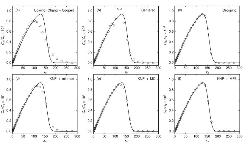
Figure 2: Long time limit cluster size distributions for the test proposed by Koiwa [45] (clustering of quenched-in vacancies) using different approximations (circles): (a) Chang-Cooper scheme (upwind scheme), (b) centered scheme, (c) grouping method (G-method), KNP with (d) minmod, (e) MC and (f) MP5 reconstructions. The exact calculation, taking into account all cluster classes, is shown by the black solid line.

As expected, the upwind method (Fig. 2-a) introduces substantial numerical diffusion and the distribution broadens. It should be noted, however, that the zeroth and first moments of the distribution are well reproduced. The error on the cluster density ($n\geq 2$) is about 5 %, while for the average number of vacancies inside clusters it is only 2 %. Owing to its simplicity and high efficiency (see below), this method is attractive if the quantity of interest is the cluster density or the average number of vacancies. However, if a precise description of the cluster distribution is needed, this scheme should be avoided. The centered scheme (Fig. 2-b) introduces spurious oscillations in the solution. It is therefore clearly inappropriate for this test, and more generally for all cases with strong advection terms. Significant improvement is obtained with the simple minmod reconstruction (Fig. 2-d): no oscillations appear and it produces less numerical diffusion than the upwind scheme. Numerical diffusion can be even more reduced by the use of MC reconstruction (Fig. 2-e), although near the peak one can still observe a small deviation with respect to the reference calculation. Among the reconstructions that were tested, MP5 clearly appears to be the best one; it perfectly reproduces the reference calculation (Fig. 2-f). Incidentally, this calculation also shows that the error due to the transformation of the master equation into a Fokker-Planck equation is completely negligible. Although the Fokker-Planck approximation is derived from a Taylor expansion of the master equation, which is strictly valid only for $n\gg 1$, we observe numerically that using this approximation for $n$ as low as 5 does not introduce error in the solution. Concerning grouping methods, the G-method (Fig. 2-c) performs very well also, the only difference with the MP5 reconstruction being the presence of unphysical negative concentrations in the large cluster size tail of the distribution (value for $x_{n}$ around 180 in Fig. 2-c). Such unphysical effects cannot appear with the MP5 reconstruction since the scheme is monotonicity preserving. We conclude from this test that the MP5 scheme is indeed very accurate.

The primary purpose of this work is to compare the accuracy of the discretization schemes. It is however instructive to compare the computation times required to perform the simulations with a given time solver. The wall-clock computation times on a single core processor are given in Tab. 2 using CVODES package. To make the comparison sensible between the different schemes, the Jacobian matrix is evaluated by CVODES using finite differences and the standard dense linear solver included in the package is used. In all cases, the computation time is rather short to reach $t=2\times 10^{5}$ s (less than 10 s), but it varies from one method to another. The shortest times are for the Chang-Cooper and centered schemes. It gradually increases with the complexity of limiters. For larger systems, linear algebra dominates the overall computation time and one can expect the efficiency of the grouping method to decrease, since it uses two equations per group, so approximately twice more equations than the Fokker-Planck based methods. A systematic study of the efficiency is however difficult to perform, since a time solver can be more or less adapted to a spatial discretization. For example, implicit methods as implemented in CVODES are probably not optimal when limiters are used, due to the frequent switches in the discretization stencils. Implicit-explicit methods, treating advective fluxes in the explicit part, may be more efficient. We emphasize however that even with CVODES, the computation time is reasonable with the MP5 scheme. If a large number of calculations are required, as for parameter fitting, it may be advantageous to use Chang-Cooper scheme or minmod limiter to get rough solutions, and then refine the final solution with the MP5 scheme.

Scheme	Computation time (s)
Chang-Cooper	1.3
Centered	1.3
Grouping	3.0
KNP + minmod	2.8
KNP + MC	4.2
KNP + MP5	9.1

Table 2: Wall-clock computation times to reach $t=2\times 10^{5}$ s with various numerical schemes, for the test proposed by Koiwa [45]. Time integration is performed on a 2.80 GHz processor using CVODES, with finite difference calculation of the Jacobian matrix and the dense linear solver included in the package.

4.2 Loop coarsening

Loop coarsening by Ostwald ripening was studied theoretically by Burton and Speight [44] and Kirchner [43] (a model known as KBS). They found that the loop distribution in the coarsening regime obeys the following law:

$$C(\rho,t)=A\frac{\rho}{(2-\rho)^{4}}\exp{\left(-\frac{4}{2-\rho}\right)}\frac{1}{\langle r(t)\rangle^{2}},$$ (32)

where $\rho=r/\langle r(t)\rangle$, $r$ is the loop radius and $\langle r(t)\rangle$ is the mean loop radius of the cluster distribution. The parameter $A$ is a normalizing constant, which can be expressed, for example, as a function of the total concentration of defects inside the loops, which remains constant during the coarsening process. For a pure prismatic loop, the loop radius $r$ is related to the number of particles $x$ by $\pi r^{2}b=xV_{\mathrm{at}}$, where $b$ is the Burgers vector.

To make the problem tractable, in addition to the classical hypotheses of the LSW theory for 3D particles [41, 42], two main approximations are made in the KBS approach in order to obtain Eq. (32):

1. The formation energy of unfaulted, circular loops is given by a simple line tension model:

   $$E^{\mathrm{f}}(r)=2\pi r\mathcal{T},$$ (33)

   where $\mathcal{T}$ is the line tension, which is considered constant. Another expression is given by Hirth and Lothe [46] using isotropic elasticity, for an isolated pure prismatic loop:

   $$E^{\mathrm{f}}(r)=2\pi r\frac{\mu b^{2}}{4\pi(1-\nu)}\left[\ln{\left(\frac{4r}{r_{\mathrm{c}}}\right)}-1\right],$$ (34)

   where $\mu$ is the shear modulus, $\nu$ is Poisson’s ratio and $r_{\mathrm{c}}$ is a core cut-off radius. Since $F_{n}^{\mathrm{b}}=E^{\mathrm{f}}_{1}+E^{\mathrm{f}}_{n-1}-E^{\mathrm{f}}_{n}$ with $E^{\mathrm{f}}_{n}=E^{\mathrm{f}}(r_{n})$ in Eq. (4), the logarithmic dependency may affect the emission rates $\alpha_{n}$ and therefore the shape of the loop distribution.

2. The diffusion flux of defects to a loop can be written as the flux to a spherical cluster of the same radius, which means that $\beta_{n}$ is given by Eq. (3) with $\pi r_{n}^{2}b=x_{n}V_{\mathrm{at}}$ (the loop is assumed to be pure prismatic). Therefore, the toroidal shape of the cluster is not taken into account. Seeger and Gösele [47] have shown that, when the diffusion problem is solved in toroidal geometry, the absorption coefficient reads

   $$\beta_{n}=2\pi r_{n}\frac{2\pi}{\ln{\left(\frac{8r_{n}}{r_{\mathrm{p}}}\right)}}D_{1},$$ (35)

   where $r_{\mathrm{p}}$ is a core cut-off radius. More accurate formulas take into account the drift-diffusion process due to the elastic interaction between the defect and the loop [48, 49].

To test the validity of the formula (32) given by the KBS theory and the sensitivity of cluster distributions to absorption rates $\beta_{n}$ and to the energetics of loops, RECD calculations were performed with different approximations:

1. Spherical model for the absorption kinetics (Eq. (3)), line tension model for the energetics of loops (Eq. (33)), as for the KBS approach.

2. Spherical model for the absorption kinetics (Eq. (3)), formula based on isotropic elasticity for the energetics of loops (Eq. (34)).

3. Toroidal model for the absorption kinetics (Eq. (35)), line tension model for the energetics of loops (Eq. (33)).

The list of parameters corresponding to loops in aluminum is given in Tab. 3. In our calculations the line tension is given by $\mathcal{T}=\kappa\mu b^{2}$, where $\kappa$ has been adjusted to give a continuous evolution for binding energies from di-vacancies, the value of which is imposed, to larger clusters, for which the line tension is used. Likewise, the value of the core cut-off radius $r_{\mathrm{c}}$ in Tab. 3 ensures a smooth transition between di-vacancies and larger loops.

Symbol	Description	Value	Unit	Reference
$V_{\mathrm{at}}$	Atomic volume	$1.648\times 10^{-29}$	m3
$b$	Burgers vector	0.2857	nm
$E^{\mathrm{m}}_{1}$	Migration energy of vacancies	0.61	eV	[50]
$D_{0,1}$	Diffusion prefactor of vacancies	$1.18\times 10^{-5}$	m2 s-1	[51]
$T$	Temperature	600	K
$\mu$	Shear modulus	26.5	GPa	[51]
$\nu$	Poisson’s ratio	0.345		[51]
$E^{\mathrm{f}}_{1}$	Formation energy of vacancies	0.67	eV	[50]
$F^{\mathrm{b}}_{2}$	Binding energy of two vacancies	0.2	eV	[50]
$\kappa$	Coefficient for the line tension	0.1
$r_{\mathrm{c}}$	Core cut-off radius for the elastic law	0.15	nm	[51]
$r_{\mathrm{p}}$	Core cut-off radius for the absorption rate	0.5713	nm

Table 3: Parameters used for the simulation of vacancy loop coarsening in aluminum.

Initial distributions are only populated for the class $n=100$ ($x_{n}\approx 391$ due to the geometric progression of the mesh), with a concentration equal to $10^{23}$ m^-3. This initial condition permits to determine the normalizing constant $A$ in (32). The use of a Fokker-Planck approach enables us to simulate cluster distributions with less than 1000 classes, whereas a simulation with all cluster classes would require approximately 16 million equations. The first 20 cluster classes are described by the master equation, then a geometric progression is used with $\epsilon=0.03$ for 100 classes and $\epsilon$ is decreased to 0.01 for the remaining classes. Calculations are performed with MP5 reconstruction up to a time at which the normalized distributions are stationary. It has been checked that it is the case for all parametrizations at $t=5$ s. In Fig. 3 (a)–(c) we show the normalized cluster distributions $\tilde{C}(\rho,t)=C(\rho,t)\langle r(t)\rangle^{2}/A$ obtained by RECD within the Fokker-Planck approach at $t=5$ s as well as the one predicted by the KBS theory.

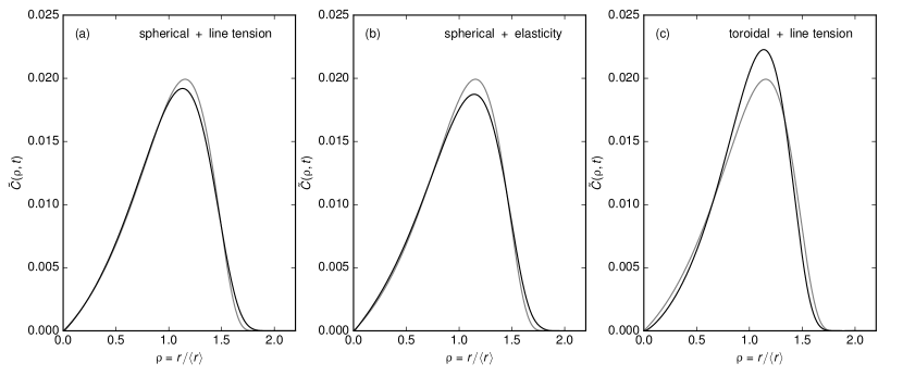
Figure 3: Distributions obtained by RECD using various approximations (black line, see text) and given by the KBS theory (gray line).

With parametrization (a), which is based on the same approximations as KBS theory, a good agreement is obtained (Fig. 3-(a)). The profile given by RECD is slightly less peaked and broader than the theoretical profile. We have checked, by varying the mesh size, that numerical diffusion is negligible and cannot explain this small discrepancy. Most probably it comes from the probabilistic nature of the growth law in RECD, whereas in KBS it is purely deterministic. In RECD, growth occurs by successive absorptions of monomers but emissions can also occur, whereas in KBS theory any cluster of size larger than the critical radius will grow. Such an argument has been put forward to explain the discrepancy between LSW theory and RECD calculations of the coarsening of 2D deposits [52]. Broader distributions were also obtained with RECD, but the difference was much more important between LSW and RECD than in the present case. Our results are also in line with the work by Senkov [53], who pointed out the role of fluctuations to explain why experimental distributions are often broader than those predicted by LSW theory.

When Eq. (34) based on isotropic elasticity is used, results are almost identical to those obtained with the simple line tension model (Fig. 3-(b)). This result is compatible with dislocation dynamics simulations of the coarsening of loops [51]: the authors obtained distributions in good agreement with KBS theory, although no assumption on the energetics of loops as in Eqs. (33) and (34) is made in this type of simulations. These results can also be compared to experimental results in silicon. Some authors found that the loop distributions followed a KBS law [54], while others found loop distributions with much longer tails [55]. They ascribed this discrepancy to the logarithmic term in Eq. (34). Although our simulations are performed on a different material, they clearly do not support this interpretation.

Interestingly, a more significant difference appears between RECD results and KBS theory if the absorption coefficient takes into account the toroidal geometry of the loop (Fig. 3-(c)). In this case, the distribution is sharper. This can be explained by the logarithmic term in Eq. (35) which decreases the absorption rate for large clusters with respect to the spherical approximation, thereby lowering their growth rate.

It should be noted that the influence of other loops on the absorption flux due to overlapping diffusion fields and on the energetics of loops is not taken into account in these calculations. More complex models would be necessary to include these effects, see e.g. [56], but this is beyond the scope of the present work. What we want to emphasize here is the importance of using a proper numerical scheme to obtain physical distributions which are not distorted by numerical diffusion, in order to compare the various physical models. Essentially, our conclusions would have been difficult, if not impossible to draw, with other numerical schemes.

5 Conclusion

In this work we have introduced a numerical scheme to accurately and efficiently solve cluster dynamics equations. It is based on a coupling between the master equation (for small clusters) and the discretization of the Fokker-Planck equation (for large clusters). To avoid the distortion of cluster distributions in the region where the Fokker-Planck equation is used, special care must be taken. We have shown that high resolution methods must be used for the advection term. More specifically, the KNP scheme coupled with the MP5 reconstruction appears to be a very attractive method. On the cases that have been tested, the results obtained by MP5 reconstruction are in very good agreement with the reference solution even when using rather large mesh sizes. The so-obtained numerical method compares favourably with the grouping methods, since it uses twice less equations and prevents the appearance of negative concentrations. In addition, the use of the Fokker-Planck equation permits to clearly identify the drift and diffusion terms, which can be interesting for physical interpretation. The method can be easily generalized to simulations containing two species by applying the algorithm along each dimension, except if cross-terms in the Fokker-Planck equation are present [11]. Such terms arise if clusters containing several species are mobile. For higher dimensions, stochastic methods are probably more appropriate due to the increase in the number of equations to solve [12, 13, 14]. It should also be noted that the method is not adapted if large clusters are mobile since it is based on a Taylor expansion, whereas grouping methods are applicable to this case [57].

Using this method, we have simulated the loop coarsening in aluminum and compared our results to the KBS theory. When the same assumptions are taken for the absorption coefficients and energetics of loops, a good agreement is obtained. Cluster distributions are found to be only slightly broader in RECD calculations, which can be ascribed to the probabilistic nature of the growth law in RECD. Additional calculations show that normalized cluster distributions do not depend much on the energetics of loops, but that they are sensitive to the model used for the absorption coefficients.

6 Acknowledgments

This work was performed within the NEEDS project MathDef (Projet Blanc). We gratefully acknowledge the financial support of NEEDS. The CRESCENDO code, which was used for this study, is developed in collaboration with EDF R&D within the framework of I3P institute.

Appendix A MP5 reconstruction

We recall here briefly the MP5 reconstruction by Suresh and Huynh [39], adapted to the case of non-uniform meshes. We assume that $F(x)$ is positive at $x_{n+1/2}$, so in view of (20) we need to determine $C_{n+1/2}^{-}$. The arguments can be easily adapted to the case $F(x)<0$.

The method proceeds in two steps that are successively detailed in A.1 and A.2 below:

1. A high order approximation of $C_{n+1/2}^{-}$ is calculated, based on the values $\{C_{j}\}_{j\in\mathbb{N}}$;

2. The value of $C_{n+1/2}^{-}$ is possibly changed (limiting process) to ensure that if the $\{C_{j}\}_{j\in\mathbb{N}}$ are initially monotone, they remain monotone at the subsequent timestep. This amounts to imposing the value of $C_{n+1/2}^{-}$ to lie inside some prescribed intervals which depend on the initial values of $\{C_{j}\}_{j\in\mathbb{N}}$. Limiting leads to a lower order reconstruction, but guarantees that no oscillations appear. Intervals can be set to impose TVD property, but it can lead to too much smearing near extrema. With MP5 reconstruction the intervals are enlarged near extrema, to keep as much as possible the initial high order approximation of $C_{n+1/2}^{-}$: although TVD property is lost in general, monotonicity is preserved and the accuracy is higher than with TVD schemes.

A.1 Original interface value

The value at the interface $C_{n+1/2}^{-}$ is defined by $C_{n+1/2}^{-}=\tilde{C}_{n}(x_{n+1/2})$, where

$$\tilde{C}_{n}(x)=\sum_{i=1}^{5}a_{i-1}\left(x-x_{n}\right)^{i-1}.$$ (36)

Following Ref. [58], the coefficients $a_{i}$ are obtained by imposing that

$$\frac{1}{\Delta x_{n+k}}\int_{I_{n+k}}\tilde{C}_{n}(x)\,\mathrm{d}x=C_{n+k}\qquad\textrm{for any }k\in[-2,1,0,1,2],$$ (37)

where $I_{n}$ is the interval corresponding to index $n$. For a uniform mesh, this leads to

$$C_{n+1/2}^{-}=\frac{1}{60}\left(2C_{n-2}-13C_{n-1}+47C_{n}+27C_{n+1}-3C_{n+2}\right).$$ (38)

Higher order reconstructions may be used [39], but in practice for cluster dynamics problems this reconstruction appears accurate enough. To determine $C_{n+1/2}^{-}$ in the non-uniform case, a linear system must be solved at each interface point for the non-uniform scheme, which makes it more complicated to implement and less efficient than the uniform scheme. For meshes with low spatial variation as those considered in the present work, we have found that the two versions lead to nearly identical results.

A.2 Slope limiter

The following steps are performed to preserve the monotonicity of the solution:

• The following values are computed:

  $$C_{n}^{\mathrm{UL}} =C_{n}+2\gamma\frac{C_{n}-C_{n-1}}{\Delta x_{n}+\Delta x_{n-1}}\Delta x_{n}$$ (39)

  $$C_{n}^{\mathrm{MP}} =C_{n}+\operatorname*{minmod}{\left(C_{n+1}-C_{n},C_{n}^{\mathrm{UL}}-C_{n}\right)},$$ (40)

  with $\gamma\geq 2$. We adopted $\gamma=4$, in agreement with Ref. [39].

• If $(C_{n+1/2}^{-}-C_{n})(C_{n+1/2}^{-}-C_{n}^{\mathrm{MP}})<0$, the value of $C_{n+1/2}^{-}$ is left unchanged. Otherwise, we must perform the limiting process which is detailed in the next step.

• If limiting is necessary, the value $C_{n+1/2}^{-}$ is changed to

  $$\operatorname*{minmod}{\left(C_{n}^{\mathrm{min}}-C_{n+1/2}^{-},C_{n}^{\mathrm{max}}-C_{n+1/2}^{-}\right)},$$

  with:

  $$C_{n}^{\mathrm{min}} =\max{\left[\min{\left(C_{n},C_{n+1},C^{\mathrm{MD}}\right)},\min{\left(C_{n},C_{n}^{\mathrm{UL}},C_{n}^{\mathrm{LC}}\right)}\right]}$$ (41)

  $$C_{n}^{\mathrm{max}} =\min{\left[\max{\left(C_{n},C_{n+1},C^{\mathrm{MD}}\right)},\max{\left(C_{n},C_{n}^{\mathrm{UL}},C_{n}^{\mathrm{LC}}\right)}\right]}$$ (42)

  $$C_{n}^{\mathrm{LC}} =C_{n}+2\frac{C_{n}-C_{n-1}}{\Delta x_{n}+\Delta x_{n-1}}\frac{\Delta x_{n}}{2}+\frac{1}{6}\zeta_{n}\operatorname*{minmod}{\left(\delta_{n-1},\delta_{n}\right)}\Delta x_{n}\left(\Delta x_{n}+\Delta x_{n-1}\right).$$ (43)

  $$C_{n}^{\mathrm{MD}} =C_{n}^{\mathrm{AV}}+\operatorname*{minmod}{\left(C_{n}^{\mathrm{FL}}-C_{n}^{\mathrm{AV}},C_{n}^{\mathrm{FR}}-C_{n}^{\mathrm{AV}}\right)}.$$ (44)

  $$C_{n}^{\mathrm{FL}} =C_{n}+\frac{C_{n}-C_{n-1}}{\Delta x_{n}+\Delta x_{n-1}}\Delta x_{n}$$ (45)

  $$C_{n}^{\mathrm{FR}} =C_{n+1}+\frac{C_{n+1}-C_{n+2}}{\Delta x_{n+1}+\Delta x_{n+2}}\Delta x_{n+1}$$ (46)

  $$C_{n}^{\mathrm{AV}} =\frac{C_{n}\Delta x_{n+1}+C_{n+1}\Delta x_{n}}{\Delta x_{n+1}+\Delta x_{n}}$$ (47)

  $$\zeta_{n} \leq\zeta_{n}^{\max}$$ (48)

  $$\zeta_{n}^{\max} =(2\gamma-1)\frac{3}{4}\frac{\Delta x_{n}+\Delta x_{n-2}+2\Delta x_{n-1}}{\Delta x_{n}+\Delta x_{n-1}}$$ (49)

  $$\delta_{n-1/2}^{\mathrm{MM}} =\operatorname*{minmod}{\left(\delta_{n-1},\delta_{n}\right)}$$ (50)

  $$\delta_{n} =\frac{8d_{n}}{(\Delta x_{n+1}+\Delta x_{n-1}+2\Delta x_{n})(\Delta x_{n}+\Delta x_{n+1})(\Delta x_{n}+\Delta x_{n-1})}$$ (51)

  $$d_{n} =C_{n-1}(\Delta x_{n+1}+\Delta x_{n})+C_{n+1}(\Delta x_{n}+\Delta x_{n-1})-C_{n}(\Delta x_{n+1}+\Delta x_{n-1}+2\Delta x_{n}).$$ (52)

For a uniform mesh and $\gamma=2$, inequality (48) leads to $\zeta_{n}\leq 9/2$, which is in line with the choice $\zeta_{n}=4$ in Ref. [39] (we recall that we have set $\gamma=4$ in this work). Reducing $\zeta_{n}$ activates limiting more often, thereby increasing stability at the cost of accuracy.

Finally, the following timestep restriction is necessary to ensure that the scheme is monotonicity preserving with an explicit Euler integration:

$$\Delta t\leq\min_{n}\left(\frac{1}{F_{n}}\frac{\Delta x_{n}}{1+\frac{2\gamma\Delta x_{n}}{\Delta x_{n}+\Delta x_{n-1}}}\right)$$ (53)

References

- Langer and Schwartz [1980] J. S. Langer, A. J. Schwartz, Phys. Rev. A 21 (1980) 948.
- Maugis and Gouné [2005] P. Maugis, M. Gouné, Acta Mater. 53 (2005) 3359.
- Soisson and Fu [2007] F. Soisson, C.-C. Fu, Phys. Rev. B 76 (2007) 214102.
- Domain et al. [2004] C. Domain, C. S. Becquart, L. Malerba, J. Nucl. Mater. 335 (2004) 121.
- Jourdan et al. [2010] T. Jourdan, J.-L. Bocquet, F. Soisson, Acta Mater. 58 (2010) 3295.
- Ortiz and Caturla [2007] C. J. Ortiz, M. J. Caturla, Phys Rev B 75 (2007) 184101.
- Clouet [2009] E. Clouet, in: D. U. Furrer, S. L. Semiatin (Eds.), Fundamentals of Modeling for Metals Processing, volume 22A of ASM Handbook, ASM International, 2009, p. 203.
- Jourdan et al. [2010] T. Jourdan, F. Soisson, E. Clouet, A. Barbu, Acta Mater. 58 (2010) 3400.
- Jourdan and Crocombette [2012] T. Jourdan, J.-P. Crocombette, Phys. Rev. B 86 (2012) 054113.
- Hairer and Wanner [1996] E. Hairer, G. Wanner, Solving Ordinary Differential Equations II: Stiff and Differential-Algebraic Problems, Springer, 1996.
- Jourdan et al. [2014] T. Jourdan, G. Bencteux, G. Adjanor, J. Nucl. Mater. 444 (2014) 298.
- Marian and Bulatov [2011] J. Marian, V. V. Bulatov, J. Nucl. Mater. 415 (2011) 84.
- Gherardi et al. [2012] M. Gherardi, T. Jourdan, S. Le Bourdiec, G. Bencteux, Comput. Phys. Commun. 183 (2012) 1966.
- Dunn and Capolungo [2015] A. Y. Dunn, L. Capolungo, Comp. Mater. Sci. 102 (2015) 314.
- Kiritani [1973] M. Kiritani, J. Phys. Soc. Jpn 35 (1973) 95.
- Golubov et al. [2001] S. I. Golubov, A. M. Ovcharenko, A. V. Barashev, B. N. Singh, Philos. Mag. A 81 (2001) 643.
- Ovcharenko et al. [2003] A. Ovcharenko, S. Golubov, C. Woo, H. Huang, Comput. Phys. Commun. 152 (2003) 208 – 226.
- Golubov et al. [2012] S. I. Golubov, A. V. Barashev, R. E. Stoller, in: R. J. Konings (Ed.), Comprehensive Nuclear Materials, Elsevier, Oxford, 2012, pp. 357 – 391.
- Waite [1957] T. R. Waite, Phys. Rev. 107 (1957) 463.
- Russel [1971] K. Russel, Acta Metallurgica 19 (1971) 753.
- Goodrich [1964] F. C. Goodrich, Proceedings of the Royal Society of London. Series A, mathematical and physical science 277 (1964) 167.
- Terrier et al. [????] P. Terrier, M. Athènes, T. Jourdan, G. Adjanor, G. Stoltz, in preparation.
- Sharafat and Ghoniem [1990] S. Sharafat, N. Ghoniem, Radiat. Eff. Defects Solids 113 (1990) 331.
- Ghoniem and Sharafat [1980] N. Ghoniem, S. Sharafat, J. Nucl. Mater. 92 (1980) 121.
- Ghoniem [1999] N. Ghoniem, Radiat. Eff. Defects Solids 148 (1999) 269.
- Turkin and Bakai [2006] A. A. Turkin, A. S. Bakai, J. Nucl. Mater. 358 (2006) 10.
- Turkin and Bakai [2007] A. A. Turkin, A. S. Bakai, Probl. At. Sci. Tech. 3 (2007) 394.
- Fletcher [1991] C. A. J. Fletcher, Computational Techniques for Fluid Dynamics 1: Fundamental and General Techniques, Springer-Verlag, Berlin, 1991.
- Ozkan and Ortoleva [2000] G. Ozkan, P. Ortoleva, J. Chem. Phys. 112 (2000) 10510.
- Chang and Cooper [1970] J. Chang, G. Cooper, J. Comput. Phys. 6 (1970) 1.
- Rempel et al. [2009] J. Y. Rempel, M. G. Bawendi, K. F. Jensen, J. Am. Chem. Soc. 131 (2009) 4479.
- Johnson [1978] R. A. Johnson, J. Nucl. Mater. 75 (1978) 77.
- Hindmarsh et al. [2005] A. C. Hindmarsh, P. N. Brown, K. E. Grant, S. L. Lee, R. Serban, D. E. Shumaker, C. S. Woodward, ACM Trans. Math. Softw. 31 (2005) 363–396.
- Hairer and Wanner [1999] E. Hairer, G. Wanner, J. Comput. Appl. Math. 111 (1999) 93.
- Leveque [2004] R. J. Leveque, Finite-Volume Methods for Hyperbolic Problems, 2004.
- Brailsford et al. [1976] A. D. Brailsford, R. Bullough, M. R. Hayns, J. Nucl. Mater. 60 (1976) 246–256.
- Kurganov et al. [2001] A. Kurganov, S. Noelle, G. Petrova, SIAM J. Sci. Comput. 23 (2001) 707–740.
- Kurganov and Tadmor [2000] A. Kurganov, E. Tadmor, J. Comput. Phys. 160 (2000) 241.
- Suresh and Huynh [1997] A. Suresh, H. T. Huynh, J. Comput. Phys. 136 (1997) 83–99.
- Ardell [1988] A. J. Ardell, in: G. W. Lorimer (Ed.), Phase transformations ’87.
- Lifshitz and Slyozov [1961] I. M. Lifshitz, V. V. Slyozov, J. Phys. Chem. Solids 19 (1961) 35.
- Wagner [1961] C. Wagner, Z. Elektrochem. 65 (1961) 581.
- Kirchner [1973] H. O. K. Kirchner, Acta Metall. 21 (1973) 85.
- Burton and Speight [1986] B. Burton, M. V. Speight, Philos. Mag. A 53 (1986) 385.
- Koiwa [1974] M. Koiwa, J. Phys. Soc. Jpn 37 (1974) 1532.
- Hirth and Lothe [1968] J. P. Hirth, J. Lothe, Theory of dislocations, McGraw-Hill, 1968.
- Seeger and Gösele [1977] A. Seeger, U. Gösele, Phys. Lett. A 61 (1977) 423.
- Dubinko et al. [2005] V. I. Dubinko, A. S. Abysov, A. A. Turkin, J. Nucl. Mater. 336 (2005) 11.
- Jourdan [2015] T. Jourdan, J. Nucl. Mater. 467 (2015) 286.
- Ehrhart et al. [1991] P. Ehrhart, P. Jung, H. Schultz, H. Ullmaier, Landolt–Börnstein, Numerical Data and Functional Relationships in Science and Technology, Atomic Defects In Metals, Springer, 1991.
- Bakó et al. [2011] B. Bakó, E. Clouet, L. M. Dupuy, M. Blétry, Philos. Mag. 91 (2011) 3173.
- Berthier et al. [2011] F. Berthier, E. Maras, I. Braems, B. Legrand, Solid State Phenom. 172-174 (2011) 664.
- Senkov [2008] O. N. Senkov, Scr. Mater. 59 (2008) 171.
- Bonafos et al. [1998] C. Bonafos, D. Mathiot, A. Claverie, J. Appl. Phys. 83 (1998) 3008.
- Pan et al. [1997] G. Z. Pan, K. N. Tu, A. Prussin, J. Appl. Phys. 81 (1997) 78.
- Brailsford and Wynblatt [1979] A. D. Brailsford, P. Wynblatt, Acta Metall 27 (1979) 489.
- Golubov et al. [2007] S. Golubov, R. Stoller, S. Zinkle, A. Ovcharenko, J. Nucl. Mater. 261 (2007) 149.
- Capdeville [2008] G. Capdeville, J. Comput. Phys. 227 (2008) 2977–3014.