On exact and optimal recovering of missing values for sequences

Abstract

The paper studies recoverability of missing values for sequences in a pathwise setting without probabilistic assumptions. This setting is oriented on a situation where the underlying sequence is considered as a sole sequence rather than a member of an ensemble with known statistical properties. Sufficient conditions of recoverability are obtained; it is shown that sequences are recoverable if there is a certain degree of degeneracy of the Z-transforms. We found that, in some cases, this degree can be measured as the number of the derivatives of Z-transform vanishing at a point. For processes with non-degenerate Z-transform, an optimal recovering based on the projection on a set of recoverable sequences is suggested. Some robustness of the solution with respect to noise contamination and truncation is established.

Key words: data recovery, discrete time, sampling theorem, band-limited interpolation.

1 Introduction

The paper studies optimal recovering of missing values for sequences, or discrete time deterministic processes. This important problem was studied intensively. The classical results for stationary stochastic processes with the spectral density $\phi$ is that a single missing value is recoverable with zero error if and only if

$$\int_{-\pi}^{\pi}\phi(\omega)^{-1}d\omega=-\infty.$$ (1)

(Kolmogorov [12], Theorem 24). Stochastic stationary Gaussian processes without this property are called minimal [12]. In particular, a process is recoverable if it is “band-limited” meaning that the spectral density is vanishing on an arc of the unit circle ${\mathbb{T}}=\{z\in{\bf C}:\ |z|=1\}$. This illustrates the relationship of recoverability with the notion of bandlimitiness or its relaxed versions such as (1). In particular, criterion (1) was extended on stable processes Peller [14] and vector Gaussian processes Pourahmadi [15].

In theory, a process can be converted into a band-limited and recoverable process with a low-pass filter. However, a ideal low-pass filter cannot be applied if there are missing values. This leads to approximation and optimal estimation of missing values. For the forecasting and other applications, it is common to use band-limited approximations of non-bandlimited underlying processes. There are many works devoted to smoothing and sampling an based on frequency properties; see e.g. Alem eta al [1], Cai [2], Candes et al [3, 4], Dokuchaev [5, 6, 7], Donoho and Stark [8], Ferreira [9, 10, 11], Kolmogorov [12], Peller [14], Pourahmadi [15, 16], Tropp [17].

The present paper also consider band-limited approximations. We consider approximation of an observed sequence in $\ell_{r}$-norms rather than matching the values at selected points. The solution is not error-free; the error can be significant if the underlying process is not band-limited. This is different from a setting in Cai [2], Candes et al [3, 4], Ferreira [11], Lee and Ferreira [13], where error-free recovering was considered. Our setting is closer to the setting from Tzschoppe and Huber [18], Zhao [20]. In Tzschoppe and Huber [18], optimization was considered as minimization of the total energy for an approximating bandlimited process within a given distance from the original process smoothed by an ideal low-pass filter. In Zhao [20], extrapolation of a band-limited process matching a finite number of points process was considered using special Slepian’s type basis in the frequency domain.

The present paper considers optimal recovering of missing values of sequences (discrete time processes) based on intrinsic properties of sequences, in the pathwise setting, without using probabilistic assumptions on the ensemble. This setting targets a scenario where a sole underlying sequence is deemed to be unique and such that one cannot rely on statistics collected from observations of other similar samples. To address this, we use a pathwise optimality criterion that does not involve an expectation on a probability space. For this setting, we obtained explicit optimal estimates for missing values of a general type processes (Theorems 1 and 2). We identified some classes of processes with degenerate Z-transforms allowing error-free recoverability (Corollary 1 and 3). For a special case of a single missing values, this gives a condition of error-free recoverability of sequences reminding classical criterion (1) for stochastic processes but based on intrinsic properties of sequences, in the pathwise setting (Corollary 3). In addition, we established numerical stability and robustness of the method with respect to the input errors and data truncation (Section 5).

2 Some definitions and background

Let ${\mathbb{Z}}$ be the set of all integers. For a set $G\subset{\mathbb{Z}}$ and $r\in[1,\infty]$, we denote by $\ell_{r}(G)$ a Banach space of complex valued sequences $\{x(t)\}_{t\in G}$ such that $\|x\|_{\ell_{r}(G)}\stackrel{{\scriptstyle{\scriptscriptstyle\Delta}}}{{=}}\left(\sum_{t\in G}|x(t)|^{r}\right)^{1/r}<+\infty$ for $r\in[1,+\infty)$, and $\|x\|_{r(G)}\stackrel{{\scriptstyle{\scriptscriptstyle\Delta}}}{{=}}\sup_{t\in G}|x(t)|<+\infty$ for $r=\infty$.

For $x\in\ell_{2}({\mathbb{Z}})$, we denote by $X={\cal Z}x$ the Z-transform

$$X(z)=\sum_{t=-\infty}^{\infty}x(t)z^{-t},\quad$$

defined for $z\in{\bf C}$ such that the series converge. For $x\in\ell_{2}({\mathbb{Z}})$, the function $X\left(e^{i\omega}\right)|_{\omega\in(-\pi,\pi]}$ is defined as an element of $L_{2}(-\pi,\pi)$. For $x\in\ell_{1}({\mathbb{Z}})$, the function $X\left(e^{i\omega}\right)$ is defined for all $\omega\in(-\pi,\pi]$ and is continuous in $\omega$.

Let $m\in{\mathbb{Z}}$ be given, $m\geq 0$. For $s\in{\mathbb{Z}}$, let $M_{s}=\{s,s+1,s+2,...,s+m\}$.

We consider data recovery problem for input processes $x\in\ell_{r}$ such that the trace $\{x(t)\}_{t\in{{\mathbb{Z}}\setminus M_{s}}}$ represents the available observations; the values $\{x(t)\}_{t\in M_{s}}$ are missing.

Definition 1.

Let ${\cal Y}\subset\ell_{r}$ be a class of sequences. We say that this class is recoverable if, for any $s\in{\mathbb{Z}}$, there exists a mapping $F:\ell_{r}({{\mathbb{Z}}\setminus M_{s}})\to{\bf R}^{m+1}$ such that $x|_{M_{s}}=F\left(x|_{{{\mathbb{Z}}\setminus M_{s}}}\right)$ for all $x\in{\cal Y}$.

For a sequence that does not belong to a recoverable class, it is natural to accept, as an approximate solution, the corresponding values of the closest process from a preselected recoverable class. More precisely, given observations $x|_{{{\mathbb{Z}}\setminus M_{s}}}$ and a recoverable class ${\cal Y}\subset\ell_{r}$, we suggest to find an optimal solution $\widehat{x}\in{\cal Y}$ of the minimization problem

$$\hbox{Minimize}\quad\sum_{t\in{{\mathbb{Z}}\setminus M_{s}}}|\widehat{x}(t)-x(t)|^{2}\quad$$

$$\hbox{over}\quad\widehat{x}\in{\cal Y},$$ (2)

and accept the trace $\widehat{x}|_{M_{s}}$ as the recovered missing values $x|_{M_{s}}$.

3 Recovering based on band-limited smoothing

We assume that we are given $\Omega\in(0,\pi)$. Let $\ell_{2}^{{\scriptscriptstyle BL},\scriptscriptstyle{\Omega}}$ be the set of all $x\in\ell_{2}({\mathbb{Z}})$ such that $X\left(e^{i\omega}\right)=0$ for $|\omega|>\Omega$ for $X={\cal Z}x$. We will call sequences $x\in\ell_{2}^{{\scriptscriptstyle BL},\scriptscriptstyle{\Omega}}$ band-limited. Let $\ell_{2}^{{\scriptscriptstyle BL},\scriptscriptstyle{\Omega}}({{\mathbb{Z}}\setminus M_{s}})$ be the subset of $\ell_{2}({{\mathbb{Z}}\setminus M_{s}})$ consisting of traces $x|_{{{\mathbb{Z}}\setminus M_{s}}}$ for all sequences $x\in\ell_{2}^{{\scriptscriptstyle BL},\scriptscriptstyle{\Omega}}$.

Proposition 1.

For any $x\in\ell_{2}^{{\scriptscriptstyle BL},\scriptscriptstyle{\Omega}}({{\mathbb{Z}}\setminus M_{s}})$, there exists a unique $\widehat{x}\in\ell_{2}^{{\scriptscriptstyle BL},\scriptscriptstyle{\Omega}}$ such that $\widehat{x}(t)=x(t)$ for $t\in{{\mathbb{Z}}\setminus M_{s}}$.

In a general case, where the sequence of observations $x|_{{\mathbb{Z}}\setminus M_{s}}$ does not necessarily represents a trace of a band-limited process, we will be using approximation described in the following lemma.

Lemma 1.

There exists a unique optimal solution $\widehat{x}\in\ell_{2}^{{\scriptscriptstyle BL},\scriptscriptstyle{\Omega}}$ of the minimization problem (2) with $r=2$ and ${\cal Y}=\ell_{2}^{{\scriptscriptstyle BL},\scriptscriptstyle{\Omega}}$.

Under the assumptions of Lemma 1, there exists a unique band-limited process $\widehat{x}$ such that the trace $\widehat{x}|_{{{\mathbb{Z}}\setminus M_{s}}}$ provides an optimal approximation of its observable trace $x|_{{{\mathbb{Z}}\setminus M_{s}}}$. The corresponding trace $\widehat{x}|_{M_{s}}$ is uniquely defined and can be interpreted as the solution of the problem of optimal recovering of the missing values $x|_{M_{s}}$ (optimal in the sense of problem (2) given $\Omega$). In this setting, the process $\widehat{x}$ is deemed to be a smoothed version of $x$, and the process $\eta=x-\widehat{x}$ is deemed to be an irregular noise. This justifies acceptance of $\widehat{x}|_{M_{s}}$ as an estimate of missing values. It can be noted that the recovered values depend on the choice of $\Omega$; the selection of $\Omega$ has to be based on some presumptions about cut-off frequencies suitable for particular applications.

Let $H(z)$ be the transfer function for an ideal low-pass filter such that $H\left(e^{i\omega}\right)={\mathbb{I}}_{[-\Omega,\Omega]}(\omega)$, where ${\mathbb{I}}$ denotes the indicator function. Let $h={\cal Z}^{-1}H$; it is known that $h(t)=\Omega\,{\rm sinc\,}(\Omega t)/\pi$; we use the notation ${\rm sinc\,}(x)=\sin(x)/x$, and we use notation $\circ$ for the convolution in $\ell_{2}({\mathbb{Z}})$. The definitions imply that $h\circ x\in\ell_{2}^{{\scriptscriptstyle BL},\scriptscriptstyle{\Omega}}$ for any $x\in\ell_{2}({\mathbb{Z}})$.

Consider a matrix ${\rm A}=\{h(k-p)\}_{k=0,p=0}^{m,m}\in{\bf R}^{(m+1)\times(m+1)}$. Let $I_{m+1}$ be the unit matrix in ${\bf R}^{(m+1)\times(m+1)}$.

Lemma 2.

The matrix $I_{m+1}-{\rm A}$ is non-degenerate.

Theorem 1.

Let $x\in\ell_{2}({\mathbb{Z}})$ and $\Omega\in(0,\pi)$. Given observations $x|_{{{\mathbb{Z}}\setminus M_{s}}}$, the problem (2) with $r=2$ and ${\cal Y}=\ell_{2}^{{\scriptscriptstyle BL},\scriptscriptstyle{\Omega}}$ has a unique optimal solution $\widehat{x}\in\ell_{2}^{{\scriptscriptstyle BL},\scriptscriptstyle{\Omega}}$ which yields an estimate of $x|_{M_{s}}$ defined as

$$\widehat{x}(s+p)=y_{p},\quad p=0,1,...,m,$$ (3)

where $y=\{y_{p}\}_{p=0}^{m}\in{\bf C}^{m+1}$ is defined as

$$y=(I_{m+1}-{\rm A})^{-1}z,$$ (4)

with $z=\{z_{p}\}_{p=0}^{m}\in{\bf C}^{m+1}$ defined as

$$z_{p}=\sum_{t\in{{\mathbb{Z}}\setminus M_{s}}}h(p-t)x(t).$$ (5)

Corollary 1.

For any $\Omega\in(0,\pi)$, the class $\ell_{2}^{{\scriptscriptstyle BL},\scriptscriptstyle{\Omega}}$ is recoverable in the sense of Definition 1.

Remark 1.

Equations (3)-(5) applied to a band-limited process $x\in\ell_{2}^{{\scriptscriptstyle BL},\scriptscriptstyle{\Omega}}$ represent a special case of the result Ferreira [9, 10]. The difference is that $x$ is Theorem 1 and (3)-(5) is not necessarily band-limited.

The case of a single missing value

It appears that the solution for the special case of a single missing value (i.e. where $m=0$) allows a convenient explicit formula.

Corollary 2.

Let $\Omega\in(0,\pi)$ and $x\in\ell_{2}({\mathbb{Z}})$ be given. Given observations $x|_{{\mathbb{Z}}\setminus\{s\}}$, the problem (2) with $r=2$ and ${\cal Y}=\ell_{2}^{{\scriptscriptstyle BL},\scriptscriptstyle{\Omega}}$ has a unique solution $\widehat{x}\in\ell_{2}^{{\scriptscriptstyle BL},\scriptscriptstyle{\Omega}}$ which yields an estimate of $x(s)$ defined as

$$\widehat{x}(s)=\frac{\Omega}{\pi-\Omega}\sum_{t\in{{\mathbb{Z}}\setminus M_{s}}}x(t){\rm sinc\,}[\Omega(s-t)].$$ (6)

This solution is optimal in the sense of problem (2) with $m=0$, $M_{s}=\{s\}$, $r=2$, and ${\cal Y}=\ell_{2}^{{\scriptscriptstyle BL},\scriptscriptstyle{\Omega}}$, given $\Omega\in(0,\pi)$.

Remark 2.

Corollary 2 applied to a band-limited process $x_{\scriptscriptstyle BL}\in\ell_{2}^{{\scriptscriptstyle BL},\scriptscriptstyle{\Omega}}$ gives a formula

$$x_{\scriptscriptstyle BL}(s)=\frac{\Omega}{\pi-\Omega}\sum_{t\in{{\mathbb{Z}}\setminus M_{s}}}x_{\scriptscriptstyle BL}(t){\rm sinc\,}[\Omega(s-t)].$$

This formula is known Ferreira [9, 10]; however, equation (6) is Corollary 2 is different since $x$ in (6) is not necessarily band-limited.

4 Recovering without smoothing

Theorem 1 suggests to replace missing values by corresponding values of a smoothed band-limited process. This process is actually different from the underlying input process; this could cause a loss of some information contained in high-frequency components. Besides, it could be difficult to justify a particular choice of $\Omega$ in (6) defining the degree of smoothing. To overcome this, we consider below the limit case where $\Omega\to\pi-0$.

Again, we consider input sequences $\{x(t)\}_{t\in{{\mathbb{Z}}\setminus M_{s}}}$ representing the observations available; the values for $t\in M_{s}$ are missing.

Without a loss of generality, we assume that either $s=0$ or $m=0$.

Let $\omega_{0}\in(0,\pi]$ be given. For $x\in\ell_{2}$, l

For $\sigma=(\sigma_{0},\sigma_{1}...,\sigma_{m})\in{\bf R}^{m+1}$ such that $\sigma_{k}\geq 0$, $k=0,1,...,m$, let

$${\cal X}_{\sigma}\stackrel{{\scriptstyle{\scriptscriptstyle\Delta}}}{{=}}\Bigl{\{}x\in\ell_{1}:\ \sum_{t\in{\mathbb{Z}}}|t|^{m}|x(t)|<+\infty,\quad\left|\frac{d^{k}X}{d\omega^{k}}\left(e^{i\omega_{0}}\right)\right|\leq\sigma_{k},$$

$$k=0,1,...,m,\quad X={\cal Z}x\Bigr{\}}.$$

Here and below we assume, as usual, that $d^{k}X/d\omega^{k}=X$ for $k=0$.

It can be shown that, for $x\in{\cal X}_{\sigma}$ and $X={\cal Z}x$, we have that the functions $\frac{d^{k}X\left(e^{i\omega}\right)}{d\omega^{k}}$ are continuous in $\omega$ for $k=0,1,...,m$.

Definition 2.

Let ${\cal X}_{0}$ be the corresponding set ${\cal X}_{\sigma}$ with $\sigma=0$, i.e. with $\sigma_{p}=0$ for $p=0,1,...,m$. We will call $x$ degenerate of order $m$.

Let us introduce a matrix ${\rm B}(\omega)=\{b_{pk}(\omega)\}_{k=0,p=0}^{m,m}\in{\bf C}^{(m+1)\times(m+1)}$ such that

$$b_{pk}(\omega)=[-i(s+k)]^{p}e^{-i\omega(s+k)},\quad\omega\in(-\pi,\pi].$$

In particular, if $m=0$, then ${\rm B}(\omega)=e^{-i\omega s}$. If $m>0$, then, by the assumptions, $s=0$ and $b_{pk}(\omega)=(-ik)^{p}e^{-i\omega k}$.

Lemma 3.

For any $\omega\in(-\pi,\pi]$, the matrix ${\rm B}(\omega)$ is non-degenerate.

Theorem 2.

Let $x\in\ell_{1}({\mathbb{Z}})$ be given such that $\sum_{t\in{\mathbb{Z}}}|t|^{m}|x(t)|<+\infty$. Given observations $x|_{{{\mathbb{Z}}\setminus M_{s}}}$, the problem (2) with $r=1$ and ${\cal Y}={\cal X}_{0}$ has a unique solution $\widehat{x}\in\ell_{2}^{{\scriptscriptstyle BL},\scriptscriptstyle{\Omega}}$ which yields an estimate of $x|_{M_{s}}$ defined as

$$\widehat{x}(s+p)=y_{p}(\omega_{0}),\quad p=0,1,...,m,$$ (7)

where $y(\omega)=\{y_{p}(\omega)\}_{p=0}^{m}\in{\bf C}^{m+1}$ is defined as

$$y(\omega)={\rm B}(\omega)^{-1}z(\omega),$$ (8)

with $z(\omega)=\{z_{p}(\omega)\}_{p=0}^{m}\in{\bf C}^{m+1}$ defined as

$$z_{p}(\omega)=-\sum_{t\in{{\mathbb{Z}}\setminus M_{s}}}(-it)^{p}e^{-i\omega t}x(t).$$ (9)

Under the assumptions of Theorem 2, there exists a unique recoverable process $\widehat{x}\in{\cal X}_{0}$ such that $\widehat{x}|_{t\in{{\mathbb{Z}}\setminus M_{s}}}=x|_{t\in{{\mathbb{Z}}\setminus M_{s}}}$. The corresponding trace $\widehat{x}|_{M_{s}}$ is uniquely defined and can be interpreted as the solution of the problem of optimal recovering of the missing values $x|_{M_{s}}$ (optimal in the sense of problem (2) for ${\cal Y}={\cal X}_{0}$). In addition, Theorem 2 implies that ${\cal X}_{0}\neq\emptyset$ for any $m\geq 0$; this follows from the implication from this theorem that a sequence from $\ell_{1}$ can be transformed into a sequence in ${\cal X}_{\sigma}$ by changing its $m$ terms.

Corollary 3.

The class ${\cal X}_{0}$ is recoverable in the sense of Definition 1 with $r=1$ and ${\cal Y}={\cal X}_{0}$.

Remark 3.

By Corollary 3 applied with $m=0$, a single missing value process $x\in\ell_{1}$ is recoverable if $X\left(e^{\omega_{0}}\right)=0$ for $X={\cal Z}x$; this reminds condition (1) for spectral density of minimal Gaussian processes [12].

The case of a single missing value

Again, the solution for the special case of a single missing value (i.e. where $m=0$ and $M_{s}=\{s\}$) allows a simple explicit formula.

Corollary 4.

Let $s\in{\mathbb{Z}}$ and $x\in\ell_{1}({\mathbb{Z}})$ be given. Given observations $x|_{{\mathbb{Z}}\setminus\{s\}}$, the problem (2) with $r=1$ and ${\cal Y}={\cal X}_{0}$ has a unique solution $\widehat{x}\in\ell_{2}^{{\scriptscriptstyle BL},\scriptscriptstyle{\Omega}}$ which yields an estimate of $x(s)$ defined as

$$\widehat{x}(s)=-\sum_{t\neq s}e^{i\omega_{0}(s-t)}x(t),$$ (10)

where the optimality is understood in the sense of problem (2) with $m=0$, $M_{s}=\{s\}$, $r=1$, and ${\cal Y}={\cal X}_{0}$.

Remark 4.

Formula (10) with $\omega_{0}=\pi$ has the form

$$\widehat{x}(s)=-\sum_{t\in{{\mathbb{Z}}\setminus M_{s}}}(-1)^{t-s}x(t).$$ (11)

This represents the limit case of formula (6), since

$$\frac{\Omega}{\pi-\Omega}{\rm sinc\,}[\Omega(s-t)]\to-(-1)^{t-s}\quad\hbox{as}\quad\Omega\to\pi-0$$

for all $t\neq s$.

Optimality in the minimax sense

It will be convenient to use mappings $\delta_{p}:{\bf C}^{m+1}\to{\bf C}$, where $p\in\{0,1,...,m\}$, such that $\delta_{p}(y)=y_{p}$ for a vector $y=(y_{0},y_{1},...,y_{m})\in{\bf C}^{m+1}$.

Proposition 2.

In addition to the optimality in the sense of problem (2) with ${\cal Y}={\cal X}_{0}$, solutions obtained in Theorems 2 and Corollalry 2 are also optimal in the following sense.

1. If $m=0$, then solution (6) is optimal in the minimax sense such that

   $$\sup_{x\in{\cal X}_{\sigma}}|\widehat{x}(s)-x(s)|\leq\sigma_{0}\leq\sup_{x\in{\cal X}_{\sigma}}|\widetilde{x}(s)-x(s)|$$ (12)

   for any estimator $\widetilde{x}(s)=F\left(x|_{{\mathbb{Z}}\setminus\{s\}}\right)$, where $F:\ell_{1}({\mathbb{Z}}\setminus\{s\})\to{\bf C}$ is a mapping.

2. If $m\geq 0$ and $s=0$, then solution (7)-(9) is optimal in the mininax sense such that

   $$\sup_{x\in{\cal X}_{\sigma}}|\delta_{p}({\rm B}(\omega_{0})\widehat{\eta})|\leq\sigma_{p}\leq\sup_{x\in{\cal X}_{\sigma}}|\delta_{p}({\rm B}(\omega_{0})\widetilde{\eta})|,\quad$$

   $$p=0,1,...,m,$$ (13)

   for any estimator $\widetilde{x}|_{M_{s}}=F\left(x|_{{\mathbb{Z}}\setminus M_{s}}\right)$, where $F:\ell_{1}({{\mathbb{Z}}\setminus M_{s}})\to{\bf C}^{m+1}$ is a mapping, $\widehat{\eta}=\{\widehat{x}(t)-x(t)\}_{t=s}^{s+m}\in{\bf C}^{m+1}$, $\widetilde{\eta}=\{\widetilde{x}(t)-x(t)\}_{t=s}^{s+m}\in{\bf C}^{m+1}$.

5 Robustness with respect to noise contamination and data truncation

Let us consider a situation where an input process $x|_{{\mathbb{Z}}\setminus M_{s}}$ is observed with an error. In other words, assume that we observe a process $x_{\eta}|_{{\mathbb{Z}}\setminus M_{s}}=x|_{{\mathbb{Z}}\setminus M_{s}}+\eta|_{{\mathbb{Z}}\setminus M_{s}}$, where $\eta$ is a noise.

For a matrix $S\in{\bf C}^{m+1}$ and $r_{1},r_{2}\in[1,+\infty]$, we denote by $\|S\|_{r_{1},r_{2}}$ the operator norm of this matrix considered as an operator $S:{\bf C}^{m+1}_{r_{1}}\to{\bf C}^{m+1}_{r_{2}}$, where ${\bf C}^{m+1}_{r}$ denote the linear normed space formed as ${\bf C}^{m+1}$ provided with $\ell_{r}$-norm.

Proposition 3.

In the notations of Theorem 1,

$$\|\widehat{x}|_{M_{s}}\|_{\ell_{\theta}(M_{s})}\leq\left\|(I_{m+1}-{\rm A})^{-1}\right\|_{2,\theta}\|x|_{{{\mathbb{Z}}\setminus M_{s}}}\|_{\ell_{2}({{\mathbb{Z}}\setminus M_{s}})}.$$

for any $\theta\in[1,+\infty]$. In particular, under the assumption of Corollary 2,

$$|\widehat{x}(s)|\leq\frac{\Omega}{\pi-\Omega}\|x\|_{\ell_{2}({{\mathbb{Z}}\setminus M_{s}})}.$$

Proposition 4.

In the notations of Theorem 2,

$$\|\widehat{x}|_{M_{s}}\|_{\ell_{\theta}(M_{s})}\leq\left\|{\rm B}(\omega_{0})^{-1}\right\|_{\infty,\theta}\sum_{t\in{{\mathbb{Z}}\setminus M_{s}}}|t|^{m}|x(t)|$$

for any $\theta\in[1,+\infty]$. In particular, under the assumption of Corollary 4,

$$|\widehat{x}(s)|\leq\|x\|_{\ell_{1}({{\mathbb{Z}}\setminus M_{s}})}.$$

Propositions 3 and 4 ensure robustness of the data recovering with respect to noise contamination and truncation. This can be shown as the following.

Let $\widehat{x}_{\eta}|_{M_{s}}$ be the sequence of corresponding values defined by (3)-(5) or (7)-(9) with $x_{\eta}|_{{\mathbb{Z}}\setminus M_{s}}$ as an input, and let $\widehat{x}|_{M_{s}}$ be the corresponding values defined by (3)-(5) or with $x|_{{\mathbb{Z}}\setminus M_{s}}$ as an input. By Proposition 3,

$$\|(\widehat{x}-\widehat{x}_{\eta})|_{M_{s}}\|_{\ell_{r}(M_{s})}\leq\|(I_{m+1}-{\rm A})^{-1}\|_{\rho,2}\|\eta\|_{\ell_{2}({{\mathbb{Z}}\setminus M_{s}})}$$ (14)

for all $\eta|_{{\mathbb{Z}}\setminus M_{s}}\in\ell_{2}({{\mathbb{Z}}\setminus M_{s}})$. In particular, under the assumption of Corollary 2, i.e. for $m=0$ and $M_{s}=\{s\}$, it follows that, in the notations of Theorem 1,

$$|\widehat{x}(s)-\widehat{x}(s)|\leq\frac{\Omega}{\pi-\Omega}\|\eta\|_{\ell_{2}({{\mathbb{Z}}\setminus M_{s}})}.$$ (15)

Similarly, Propositions 4 implies that

$$|\widehat{x}(s)-\widehat{x}_{\eta}(s)|\leq\|z_{\eta}(\omega_{0})\|_{\ell_{1}({{\mathbb{Z}}\setminus M_{s}})}$$ (16)

for all $\eta|_{{\mathbb{Z}}\setminus M_{s}}\in\ell_{1}({{\mathbb{Z}}\setminus M_{s}})$, under the assumptions of this theorem, with $z_{\eta}(p,\omega)=\{z_{\eta}(p,\omega)\}_{p=0}^{m}\in{\bf C}^{m+1}$ defined as

$$z_{\eta}(p,\omega)=-\sum_{t\in{{\mathbb{Z}}\setminus M_{s}}}(-it)^{p}e^{-i\omega t}\eta(t).$$

This demonstrates some robustness of the method with respect to the noise in the observations. In particular, this ensures robustness of the estimate with respect to truncation of the input processes, such that infinite sequences $x\in\ell_{r}({{\mathbb{Z}}\setminus M_{s}})$, $r\in\{1,2\}$, are replaced by truncated sequences $x_{\eta}(t)=x(t){\mathbb{I}}_{\{|t|\leq q\}}$ for $q>0$; in this case $\eta(t)={\mathbb{I}}_{|t|>q}x(t)$. Clearly, $\|\eta\|_{\ell_{r}({{\mathbb{Z}}\setminus M_{s}})}\to 0$ as $q\to+\infty$. This overcomes principal impossibility to access infinite sequences of observations.

The experiments with sequences generated by Monte-Carlo simulation demonstrated a good numerical stability of the method; the results were quite robust with respect to deviations of input processes and truncation.

On a choice between recovering formulae (6) and (10)

It can be seen from (14) and (16) that recovering formula (10) is less robust with respect to data truncation and the noise contamination than recovering formula (6). In addition, recovering formula (10) is not applicable to $x\in\ell_{2}({\mathbb{Z}})\setminus\ell_{1}({\mathbb{Z}})$. On the other hand, application of (10) does not require to select $\Omega$. In practice, numerical implementation requires to replace a sequence $\{x(t)\}$ by a truncated sequence $x(t){\mathbb{I}}_{\{t:\ |t|\leq q\}}$; technically, this means that both formulas could be applied. The choice between (6) and (10) and of a particular $\Omega$ for (6) should be done based on the purpose of the model. In general, a more numerically robust result can be achieved with choice of a smaller $\Omega$.

This can be illustrated with the following example for a case of a single missing value. Consider a band-limited input $x\in\ell_{2}^{{\scriptscriptstyle BL},\scriptscriptstyle{\Omega}}$ with a missing value $x(0)$ (i.e, $m=0$ and $s=0$, in the notations above). In theory, application of (6) with $\Omega$ replaced by $\Omega_{1}\in(\Omega,\pi]$ produces error-free recovering, i.e. $\widehat{x}(0)=x(0)$. However, application of (6) with $\Omega$ replaced by $\Omega_{2}\in(0,\Omega_{1})$ may lead to a large error $\widehat{x}(0)-x(0)$.

On the other hand, application of (10), where $\Omega$ is not used, performs better than (6) with too small miscalculated $\Omega_{1}$. This is illustrated by Figure 1 that shows an example of a process $x(t)\in\ell_{2}^{{\scriptscriptstyle BL},\scriptscriptstyle{\Omega}}$ with $\Omega=0.1\pi$ and recovered values $\widehat{x}(0)$ corresponding to band-limited extensions obtained from (6) with $\Omega=0.1\pi$ and $\Omega=0.05\pi$. In addition, this figure shows $\widehat{x}(0)$ calculated by (10).

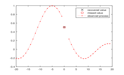
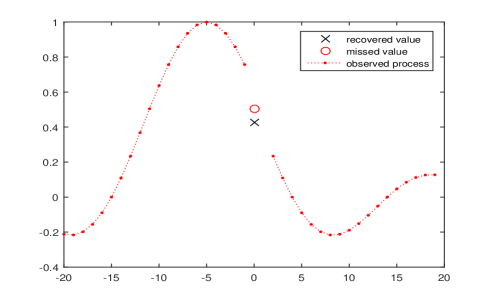
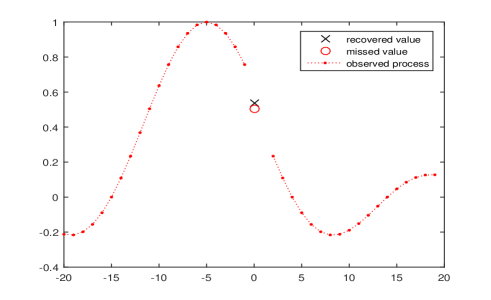
Figure 1: Example of a path $x\in\ell_{2}^{{\scriptscriptstyle BL},\scriptscriptstyle{\Omega}}$ with $\Omega=0.1\pi$ and the recovered values $\widehat{x}(0)$ calculated using 100 observations: (i) calculated by (6) for $\Omega=0.1\pi$ (top); (ii) calculated by (6) with $\Omega=0.05\pi$ (middle); (iii) calculated by (10) (bottom).

On the hand, the presence of a noise in processes that are nor recoverable without error may lead to a larger error for estimate (10). This is illustrated by Figure 2 that shows an example of a noisy process $x$ and recovered values $\widehat{x}(0)$ corresponding to band-limited extensions obtained from (6) with $\Omega=0.1\pi$ and $\Omega=0.05\pi$. In addition, this figure shows $\widehat{x}(0)$ calculated by (10).

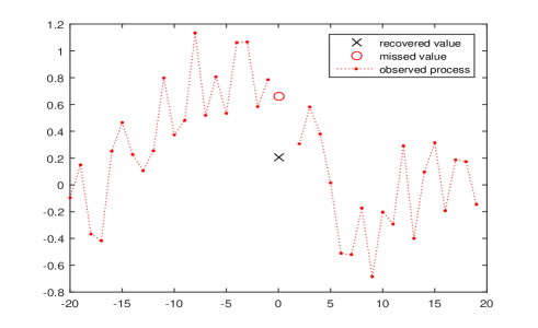
Figure 2: Example of a path $x\in\ell_{2}({{\mathbb{Z}}\setminus M_{s}})$ and the recovered values $\widehat{x}(0)$ calculated using 100 observations: (i) calculated by (6) for $\Omega=0.1\pi$ (top); (ii) calculated by (6) with $\Omega=0.05\pi$ (middle); (iii) calculated by (10) (bottom).

In these experiments, we used $M_{s}=\{0\}$ and truncated sums (6) and (10) with 100 members.

6 Proofs

Proof of Proposition 1. It is known Ferreira [9, 10, 11] that a continuous time bandlimited function can be recovered without error from an oversampling sequence where a finite number of sample values is unknown. This implies that if $x\in\ell_{2}^{{\scriptscriptstyle BL},\scriptscriptstyle{\Omega}}$ is such that $x(t)=0$ for $t\in{{\mathbb{Z}}\setminus M_{s}}$, then $x\equiv 0$. Then the proof of Proposition 1 follows. $\Box$

Proof of Lemma 1. It suffices to prove that $\ell_{2}^{{\scriptscriptstyle BL},\scriptscriptstyle{\Omega}}({{\mathbb{Z}}\setminus M_{s}})$ is a closed linear subspace of $\ell_{2}({{\mathbb{Z}}\setminus M_{s}})$. In this case, there exists a unique projection $\widehat{x}|_{{{\mathbb{Z}}\setminus M_{s}}}$ of $x|_{{{\mathbb{Z}}\setminus M_{s}}}$ on $\ell_{2}^{{\scriptscriptstyle BL},\scriptscriptstyle{\Omega}}({{\mathbb{Z}}\setminus M_{s}})$, and the proof will be completed.

Let ${\mathbb{B}}$ be the set of all mappings $X:{\mathbb{T}}\to{\bf C}$ such that $X\left(e^{i\omega}\right)\in L_{2}(-\pi,\pi)$ and such that $X\left(e^{i\omega}\right)=0$ for $|\omega|>\Omega$ for $X=\ Zx$.

Consider the mapping $\zeta:{\mathbb{B}}\to\ell_{2}^{{\scriptscriptstyle BL},\scriptscriptstyle{\Omega}}({{\mathbb{Z}}\setminus M_{s}})$ such that

$$x(t)=(\zeta(X))(t)=\frac{1}{2\pi}\int_{-\pi}^{\pi}X\left(e^{i\omega}\right)e^{i\omega t}d\omega,\quad t\in{{{\mathbb{Z}}\setminus M_{s}}}.$$

It is a linear continuous operator. By Proposition 1, it is a bijection.

Since the mapping $\zeta:{\mathbb{B}}\to\ell_{2}^{{\scriptscriptstyle BL},\scriptscriptstyle{\Omega}}({{\mathbb{Z}}\setminus M_{s}})$ is continuous, it follows that the inverse mapping $\zeta^{-1}:\ell_{2}^{{\scriptscriptstyle BL},\scriptscriptstyle{\Omega}}({{\mathbb{Z}}\setminus M_{s}})\to{\mathbb{B}}$ is also continuous; see e.g. Corollary in Ch.II.5 Yosida [19], p. 77. Since the set ${\mathbb{B}}$ is a closed linear subspace of $L_{2}(-\pi,\pi)$, it follows that $\ell_{2}^{{\scriptscriptstyle BL},\scriptscriptstyle{\Omega}}({{\mathbb{Z}}\setminus M_{s}})$ is a closed linear subspace of $\ell_{2}({{\mathbb{Z}}\setminus M_{s}})$. Then a solution $\widehat{x}$ of problem (2) is such that $\widehat{x}|_{D}$ is a projection of $x|_{D}$ on $\ell_{2}^{{\scriptscriptstyle BL},\scriptscriptstyle{\Omega}}({{\mathbb{Z}}\setminus M_{s}})$ which is unique. Then the proof of Lemma 1 follows. $\Box$

Proof of Lemma 2. Let $\bar{y}=\{\bar{y}_{k}\}_{k=0}^{m}\in{\bf C}^{m+1}$ be arbitrarily selected such that $\|\bar{y}\|_{\ell_{2}}\neq 0$. Let $y\in\ell_{2}({\mathbb{Z}})$ be such that $y|_{{{\mathbb{Z}}\setminus M_{s}}}=0$ and that $\bar{y}=y|_{M}$. In this case, $y\notin\ell_{2}^{{\scriptscriptstyle BL},\scriptscriptstyle{\Omega}}$; it follows, for instance, from Proposition 1. Let $Y={\cal Z}y$. We have that ${\cal Z}(h\circ y)=H\left(e^{i\omega}\right)Y\left(e^{i\omega}\right)$. Hence $\|H\left(e^{i\omega}\right)Y\left(e^{i\omega}\right)\|_{L_{2}(-\pi,\pi)}<\|Y\left(e^{i\omega}\right)\|_{L_{2}(-\pi,\pi)}$. This implies that $\|h\circ y\|_{\ell_{2}}<\|y\|_{\ell_{2}}$. Hence

$$\|{\rm A}\bar{y}\|_{\ell_{2}}=\|{\mathbb{I}}_{M}(h\circ y)\|_{\ell_{2}}\leq\|h\circ y\|_{\ell_{2}}<\|y\|_{\ell_{2}}=\|\bar{y}\|_{\ell_{2}}.$$

Since the space $\ell_{2}(M)$ is finite dimensional, it follows that $\|{\rm A}\|_{2,2}<1$. Then the statement of Lemma 2 follows. $\Box$

Proof of Theorem 1. Assume that the input sequences $\{x(t)\}_{t\in{{\mathbb{Z}}\setminus M_{s}}}$ are extended on $M_{s}$ such that $x|_{M_{s}}=\widehat{x}|_{M_{s}}$, where $\widehat{x}$ is the optimal process that exists according to Lemma 1. Then $\widehat{x}$ is a unique solution of the minimization problem

$$\hbox{Minimize}\quad\sum_{t\in{\mathbb{Z}}}|x_{\scriptscriptstyle BL}(t)-x(t)|^{2}\quad$$

$$\hbox{over}\quad x_{\scriptscriptstyle BL}\in\ell_{2}^{{\scriptscriptstyle BL},\scriptscriptstyle{\Omega}}.$$ (17)

By the property of the low-pass filters, $\widehat{x}=h\circ x$. Hence the optimal process $\widehat{x}\in\ell_{2}^{{\scriptscriptstyle BL},\scriptscriptstyle{\Omega}}$ from Lemma 1 is such that

$$\widehat{x}=h\circ\left(x{\mathbb{I}}_{{{\mathbb{Z}}\setminus M_{s}}}+\widehat{x}{\mathbb{I}}_{M_{s}}\right).$$

Hence

$$\widehat{x}(t)=\sum_{s\in{{\mathbb{Z}}\setminus M_{s}}}h(t-s)x(s)+\sum_{s\in M_{s}}h(t-s)\widehat{x}(s).$$ (18)

This gives that

$$x(t)-\sum_{s\in M_{s}}{\rm A}_{t,s}x(s)=z_{t}.$$

This gives (3)-(5). $\Box$

Proof of Corollary 1. If $x\in\ell_{2}^{{\scriptscriptstyle BL},\scriptscriptstyle{\Omega}}$, then $\widehat{x}=x$, since it is a solution of (2). By Theorem 1, $\widehat{x}$ is obtained as is required in Definition 1 with $r=2$ and ${\cal Y}=\ell_{2}^{{\scriptscriptstyle BL},\scriptscriptstyle{\Omega}}$. $\Box$

Proof of Lemma 3. The case where $m=0$ is trivial, since ${\rm B}(\omega)=e^{-\omega s}$ in this case. Let us consider the case where $m>0$; by the assumptions, $s=0$ in this case. Suppose that there exists $\omega\in(-\pi,\pi]$ such that the matrix ${\rm B}(\omega)$ is degenerate. In this case, there exists $q=\{q(k)\}_{k=0}^{m}\in{\bf C}^{m+1}$ such that $q\neq 0$ and ${\rm B}(\omega)y=0$. Let $Q(z)\stackrel{{\scriptstyle{\scriptscriptstyle\Delta}}}{{=}}\sum_{k=s}^{s+m}q(k)z^{k}=\sum_{k=0}^{m}q(k)z^{k}$, $z\in{\bf C}$. By the definition of ${\rm B}(\omega)$, it follows that $\frac{d^{p}Q}{d\omega^{p}}\left(e^{i\omega}\right)=0$ for $p=0,1,...,m$. Hence $\frac{d^{p}Q}{dz^{p}}(z_{0})=0$ at $z_{0}=e^{i\omega}$ for $p=0,1,...,m$. Hence $Q\equiv 0$. Therefore, the vector $q$ cannot be non-zero. This completes the proof. $\Box$

Proof of Theorem 2. Let $y\in\ell_{1}$ be selected such that $y(t)=x(t)$ for $t\notin M_{s}$ and $y|_{M_{s}}=0$. Let $Y={\cal Z}y$, and let $\widehat{x}\in\ell_{1}$ be selected such that $\widehat{x}(t)=x(t)$ for $t\notin M_{s}$, with some choice of $\widehat{x}|_{M_{s}}$. Let $\widehat{X}={\cal Z}\widehat{x}$. It follows from the definitions that

$$\frac{d^{p}\widehat{X}}{d\omega^{p}}\left(e^{i\omega}\right)=\frac{d^{p}Y}{d\omega^{p}}\left(e^{i\omega}\right)+\sum_{t=s}^{s+m}(-i\omega t)^{p}e^{-i\omega t}\widehat{x}(t)$$

$$=-z_{p}(\omega)+\delta_{p}({\rm B}(\omega)y(\omega)),\quad p=0,1,...,m.$$

For $\omega=\omega_{0}$, this gives ${\rm B}(\omega_{0})y(\omega_{0})=z(\omega_{0})$. Hence there is a unique choice that ensures that $\widehat{x}\in{\cal X}_{0}$ and $\widehat{x}|_{{\mathbb{Z}}\setminus M_{s}}=x|_{{\mathbb{Z}}\setminus M_{s}}$; this choice is defined by equations (7)-(9). Clearly, this is a unique optimal solution of the minimization problem (13) with $r=1$ and ${\cal Y}={\cal X}_{0}$. This completes the proof of Theorem 2. $\Box$

Proof of Proposition 2. It suffices to prove statement (ii) only, since statment (i) is its special case. Let $x\in{\cal X}_{\sigma}$ for some $\sigma\neq 0$, and let $Y\left(e^{i\omega}\right)=\sum_{k\in{{\mathbb{Z}}\setminus M_{s}}}e^{-i\omega k}x(k)$, $\omega\in(-\pi,\pi]$; this function is observable. By the definitions, it follows that

$$X\left(e^{i\omega}\right)=Y\left(e^{i\omega}\right)+\sum_{t\in M_{s}}e^{-i\omega k}x(t)$$

and

$$\frac{d^{p}X}{d\omega^{p}}\left(e^{i\omega}\right)=\frac{d^{p}Y}{d\omega^{p}}\left(e^{i\omega}\right)+\delta_{p}({\rm B}(\omega)y(\omega)),\quad p=0,1,...,m.$$

For $\omega=\omega_{0}$, it gives

$$\xi=-z(\omega_{0})+{\rm B}(\omega_{0})y(\omega_{0}),$$

where $\xi=\{\xi_{p}\}_{p=0}^{m}\in{\bf C}^{m+1}$ has components $\xi_{p}=\frac{d^{p}X}{d\omega^{p}}\left(e^{i\omega_{0}}\right)$ such that $|\xi_{p}|\leq\sigma_{p}$. Using the estimator from Theorem 2, we accept the value $\widehat{y}(\omega_{0})={\rm B}(\omega_{0})^{-1}z(\omega_{0})$ as the estimate of $y(\omega_{0})=\{x(s+p)\}_{p=0}^{m}$. We have that ${\rm B}(\omega_{0})y(\omega_{0})-{\rm B}(\omega_{0})\widehat{y}(\omega_{0})=\xi$. It follows that the first inequality in (13) holds. If $\sigma=0$ then the estimator is error-free.

Let us show that the second inequality in (13) holds. Suppose that we use another estimator $\widetilde{x}(s)=\widetilde{F}\left(x|_{{\mathbb{Z}}\setminus M_{s}}\right)$, where $\widetilde{F}:\ell_{2}({{\mathbb{Z}}\setminus M_{s}})\to{\bf C}$ is some mapping. Let $p\in\{0,1,...,m\}$, and let $X_{\pm}\left(e^{i\omega}\right)$ be such that $\delta_{k}({\rm B}(\omega)y(\omega))=\pm\sigma_{k}{\mathbb{I}}_{\{k=p\}}$, $k\in\{0,1,...,m\}$, and $x_{\pm}(t)=0$ for $t\in{{\mathbb{Z}}\setminus M_{s}}$ for $x_{\pm}={\cal Z}^{-1}X_{\pm}$. By the definition of ${\rm B}(\omega)$, it follows $\frac{d^{k}X_{\pm}}{d\omega^{k}}\left(e^{i\omega}\right)=\pm\sigma_{k}{\mathbb{I}}_{\{k=p\}}$. Clearly, $x_{\pm}\in{\cal X}_{\sigma}$. Moreover, we have that $\widetilde{x}_{-}|_{M_{s}}=\widetilde{x}_{+}|_{M_{s}}$ for $\widetilde{x}_{\pm}=\widetilde{F}\left(x_{\pm}|_{{\mathbb{Z}}\setminus M_{s}}\right)$, for any choice of $\widetilde{F}$, and

$$\max(|\delta_{p}({\rm B}(\omega_{0})\eta_{-})|,|\delta_{p}({\rm B}(\omega_{0})\eta_{+})|)\geq\sigma_{p},$$

$$\quad p=0,1,...,m,$$

where $\eta_{-}=\{\widetilde{x}_{-}(t)-x_{-}(t)\}_{t=s}^{s+m}\in{\bf C}^{m+1}$, $\eta_{+}=\{\widetilde{x}_{+}(t)-x_{+}(t)\}_{t=s}^{s+m}\in{\bf C}^{m+1}$. Then the second inequality in (13) and the proof of Proposition 2 follow. $\Box$

Proof of Corollary 3. If $x\in{\cal X}_{0}$, then $\widehat{x}=x$ since it is a solution of (2). By Theorem 2, $\widehat{x}$ is obtained as is required in Definition 1 with $r=1$ and ${\cal Y}={\cal X}_{0}$. $\Box$

Proof of Proposition 3. By Theorem 1,

$$\|\widehat{x}|_{M_{s}}\|_{\ell_{\theta}(M_{s})}\leq\|(I_{m+1}-{\rm A})^{-1}\|_{2,\theta}\|z\|_{\ell_{2}(M_{s})}.$$

In addition,

$$\|z\|_{\ell_{2}(M_{s})}\leq\|{\mathbb{I}}_{M_{s}}(h\circ x{\mathbb{I}}_{{{\mathbb{Z}}\setminus M_{s}}})\|_{\ell_{2}({\mathbb{Z}})}\leq\|x|_{{{\mathbb{Z}}\setminus M_{s}}}\|_{\ell_{2}({{\mathbb{Z}}\setminus M_{s}})}.$$

Then the proof of Proposition 3 follows. $\Box$

Proof of Proposition 4. By Theorem 2,

$$\|\widehat{x}|_{M_{s}}\|_{\ell_{\theta}(M_{s})}\leq\|{\rm B}(\omega_{0})^{-1}\|_{\rho,\theta}\|z(\omega_{0})\|_{\ell_{\rho}({{\mathbb{Z}}\setminus M_{s}})}.$$

Further,

$$|z_{p}(\omega_{0})|\leq\sum_{t\in{{\mathbb{Z}}\setminus M_{s}}}|t|^{m}|x(t)|.$$

Then the proof of Proposition 3 follows. $\Box$

7 Discussion and possible modifications

The present paper is focused on theoretical aspects of possibility to recover missing values. The paper suggests frequency criteria of error-free recoverability of a single missing value in pathwise deterministic setting. In particular, $m$ missing values can be recovered for processes that are degenerate of order $m$ (Definition 2). Corollary 3 gives a recoverability criterion reminding the classical Kolmogorov’s criterion (1) for the spectral densities Kolmogorov [12]. However, the degree of similarity is quite limited. For instance, if a stationary Gaussian process has the spectral density $\phi(\omega)\geq{\rm const\,}\cdot(\pi^{2}-\omega^{2})^{\nu}$ for $\nu\in(0,1)$, then, according to criterion (1), this process is not minimal Kolmogorov [12], i.e. this process is non-recoverable. On the other hand, Corollary 3 imply that single values of processes $x\in\ell_{1}$ are recoverable if $X(-1)=0$ for $X={\cal Z}x$. In particular, this class includes sequences $x$ such that $|X\left(e^{i\omega}\right)|\leq{\rm const\,}\cdot(\pi^{2}-\omega^{2})^{\nu}$ for $\nu\in(0,1)$. Nevertheless, this similarity still could be used for analysis of the properties of pathwise Z-transforms for stochastic Gaussian processes. In particular, assume that $y=\{y(t)\}_{t\in{\mathbb{Z}}}$ is a stochastic stationary Gaussian process with spectral density $\phi$ such that (1) does not hold. It follows that adjusted paths $\{(1+\delta t^{2})^{-1}y(t)\}_{t\in{\mathbb{Z}}}$, where $\delta>0$, cannot belong to $\ell_{2}^{{\scriptscriptstyle BL},\scriptscriptstyle{\Omega}}$ or ${\cal X}_{0}$. We leave this analysis for the future research.

There are some other open questions. The most challenging problem is to obtain pathwise necessary conditions of recoverability that are close enough to sufficient conditions. In addition, there are more technical questions. In particular, it is unclear if it possible to relax conditions of recoverability described as weighted $\ell_{1}$-summarability presented in the definition for ${\cal X}_{\sigma}$. It is also unclear if it is possible to replace the restrictions on the derivatives of Z-transform imposed at one common point for the processes from ${\cal X}_{0}$ by conditions at different points. We leave this for the future research.

Acknowledgment

This work was supported by ARC grant of Australia DP120100928 to the author. In addition, the author thanks the anonymous referees for their valuable suggestions which helped to improve the paper.

References

Alem eta al [2014]
Y. Alem, Z. Khalid, R.A. Kennedy. (2014).
Band-limited extrapolation on the sphere for signal reconstruction in the presence of noise, Proc. IEEE Int. Conf.
ICASSP’2014, pp. 4141-4145.
Cai [2009]
T. Cai, G. Xu, and J. Zhang. (2009), On recovery of sparse signals via
minimization, IEEE Trans. Inf. Theory, vol. 55, no. 7, pp. 3388-3397.
Candes et al [2006a]
E. Candés, T. Tao. (2006), Near optimal signal recovery from random projections: Universal encoding strategies?
IEEE Transactions on Information Theory 52(12) (2006), 5406-5425.
Candes et al [2006b]
E.J. Candes, J. Romberg, T. Tao. (2006).
Robust uncertainty principles: Exact signal reconstruction from highly incomplete frequency information.
IEEE Transactions on Information Theory52 (2), 489–509.
Dokuchaev [2010a] N. Dokuchaev. (2012). On predictors for band-limited and
high-frequency time series. Signal Processing92, iss.
10, 2571-2575.
Dokuchaev [2012b]
N. Dokuchaev. (2012). Predictors for discrete time processes with
energy decay on higher frequencies. IEEE Transactions on Signal
Processing60, No. 11, 6027-6030.
Dokuchaev [2016] N. Dokuchaev. (2016). Near-ideal causal smoothing filters for the real sequences. Signal Processing118, iss. 1, pp. 285-293.
Donoho and Stark [1989]
D. L. Donoho and P. B. Stark. (1989). Uncertainty principles and signal recovery.
SIAM J. Appl. Math., vol. 49, no. 3, pp. 906–931.
Ferreira [1992]
P.J.S.G. Ferreira. (1992). Incomplete sampling series and the recovery of missing samples
from oversampled band-limited signals, IEEE Transactions on signal processing,
40(1), pp.225–227.
Ferreira [1994a] P.J.S.G. Ferreira. (1994). The stability of a procedure for the recovery of lost samples in
band-limited signals, Signal Processing, 40(2-3), pp.195-205.
Ferreira [1994] P. G. S. G.
Ferreira (1994).
Interpolation and the discrete Papoulis-Gerchberg algorithm. IEEE Transactions on Signal Processing42 (10), 2596–2606.
Kolmogorov [1941]
A.N. Kolmogorov. (1941).
Interpolation and extrapolation of stationary stochastic series.
Izv. Akad. Nauk SSSR Ser. Mat., 5:1, 3–14.
Lee and Ferreira [2014]
D.G. Lee, P.J.S.G. Ferreira. (2014). Direct construction of superoscillations. IEEE Transactions on Signal processing, V. 62, No. 12,3125-3134.
Peller [2000] V. V. Peller (2000). Regularity conditions for vectorial stationary processes.
In: Complex Analysis, Operators, and Related Topics. The S.A. Vinogradov Memorial Volume. Ed. V. P. Khavin and N. K. Nikol’skii. Birkhauser Verlag, pp
287-301.
Pourahmadi [1984]
M. Pourahmadi (1984). On minimality and interpolation of harmonizable stable processes.
SIAM Journal on Applied Mathematics, Vol. 44, No. 5, pp. 1023–1030.
Pourahmadi [1989]
M. Pourahmadi. Estimation and interpolation of missing values of a stationary time series. J. Time Ser. Anal., 10 (1989), pp. 149-169
Tropp [2007]
J. Tropp and A. Gilbert. (2007). Signal recovery from partial information via
orthogonal matching pursuit, IEEE Trans. Inf. Theory, vol. 53, no. 12,
pp. 4655–4666.
Tzschoppe and Huber [2009]
R. Tzschoppe, J.B. Huber. (2009). Causal discrete-time system approximation of non-bandlimited continuous-time systems by means of discrete prolate spheroidal wave functions. Eur. Trans. Telecomm.20, 604–616.
Yosida [1965] K. Yosida. (1965). Functional Analysis. Springer, Berlin Heilderberg New York.
[20]
H. Zhao, R. Wang, D. Song, T. Zhang, D. Wu. (2014). Extrapolation of discrete bandlimited signals in linear canonical transform domain
Signal Processing94, 212–218.