The scaling limit of critical Ising interfaces is $\mathrm{CLE}_{3}$

Abstract.

In this paper, we consider the set of interfaces between $+$ and $-$ spins arising for the critical planar Ising model on a domain with $+$ boundary conditions, and show that it converges towards nested CLE₃.

Our proof relies on the study of the coupling between the Ising model and its random cluster (FK) representation, and of the interactions between FK and Ising interfaces. The main idea is to construct an exploration process starting from the boundary of the domain, to discover the Ising loops and to establish its convergence to a conformally invariant limit. The challenge is that Ising loops do not touch the boundary; we use the fact that FK loops touch the boundary (and hence can be explored from the boundary) and that Ising loops in turn touch FK loops, to construct a recursive exploration process that visits all the macroscopic loops.

A key ingredient in the proof is the convergence of Ising free arcs to the Free Arc Ensemble (FAE), established in [BDH16]. Qualitative estimates about the Ising interfaces then allow one to identify the scaling limit of Ising loops as a conformally invariant collection of simple, disjoint $\mathrm{SLE}_{3}$-like loops and thus by the Markovian characterization of [ShWe12] as a $\mathrm{CLE}_{3}$.

A technical point of independent interest contained in this paper is an investigation of double points of interfaces in the scaling limit of critical FK-Ising. It relies on the technology of [KeSm12].

1. Introduction

1.1. Schramm-Loewner Evolution

The introduction of Schramm’s SLE curves [Sch00] opened the road to decisive progress towards the understanding of 2D statistical mechanics. The $\left(\mathrm{SLE}_{\kappa}\right)_{\kappa>0}$ form a one-parameter family of conformally invariant random curves that are the natural candidates for the scaling limits of interfaces found in critical lattice models, as shown by Schramm’s principle [Sch00]: if a random curve is conformally invariant and satisfies the domain Markov property, then it must be an $\mathrm{SLE}_{\kappa}$ for some $\kappa>0$. The convergence of lattice model curves to SLE has been established in a number of cases, in particular for the loop-erased random walk ($\kappa=2$) and the uniform spanning tree ($\kappa=8$) [LSW04], percolation ($\kappa=6$) [Smi01], the Ising model ($\kappa=3$) and FK-Ising ($\kappa=16/3$) [CDHKS14], and the discrete Gaussian free field $\left(\kappa=4\right)$ [ScSh09].

The development of SLE has had rich ramifications, in particular the introduction of the Conformal Loop Ensembles (CLE) [She09]. The $\left(\mathrm{CLE}_{\kappa}\right)_{\kappa\in(\frac{8}{3},8]}$ are conformally invariant collections of $\mathrm{SLE}_{\kappa}$-like random loops; they conjecturally describe the full set (rather than a fixed marked set) of macroscopic interfaces appearing in discrete models. For percolation, the convergence of the full set of interfaces to $\mathrm{CLE}_{6}$ has been established [CaNe07b]. For the Gaussian free field, the connection with $\mathrm{CLE}_{4}$ is established in [MS16, ASW16]. For the random-cluster (FK) representation of the Ising model, the convergence of boundary-touching interfaces to a subset of CLE_16/3 has been established in [KeSm15]. This paper shows convergence of Ising interfaces to CLE₃, and this is the first convergence result in the non boundary touching regime $\kappa\leq 4$.

1.2. Ising Interfaces and SLE

The Ising model is the most classical model of equilibrium statistical mechanics. It consists of random configurations of $\pm 1$ spins on the vertices of a finite graph $\mathcal{G}$, which interact with their neighbors: the probability of a spin configuration $\left(\sigma_{x}\right)_{x\in V}$ is proportional to $\exp\left(-\beta H\left(\sigma\right)\right)$, where the energy $H\left(\sigma\right)$ is given by $-\sum_{x\sim y}\sigma_{x}\sigma_{y}$ and $\beta$ is a positive parameter called the inverse temperature.

The two-dimensional Ising model (i.e. when $\mathcal{G}\subset\mathbb{Z}^{2}$) has been the subject of intense mathematical and physical investigations. A phase transition occurs at the critical value $\beta_{c}=\frac{1}{2}\ln\left(\sqrt{2}+1\right)$: for $\beta<\beta_{c}$ the spins are disordered at large distances, while for $\beta>\beta_{c}$ a long range order is present. Thanks to the exact solvability of the model, much is known about the phase transition of the model; the recent years have in particular seen important progress towards understanding rigorously the scaling limit of the fields [Hon10, HoSm13, CHI15, HKV17] and the interfaces [Smi06, CDHKS14, BDH16] of the model at the critical temperature $\beta_{c}$.

For the two-dimensional Ising model, we call spin interfaces the curves that separate the $+$ and $-$ spins of the model (as a technical aside, one needs to make choices when trying to follow an Ising interface on the square lattice, however these discrete choices are irrelevant in the scaling limit). In the case of Dobrushin boundary conditions (i.e. $+$ spins on a boundary arc and $-$ spins on the boundary complement) the resulting distinguished spin interface linking boundary points can be shown to converge to $\mathrm{SLE}_{3}$ [CDHKS14], using the discrete complex analysis of lattice fermions [Smi10a, ChSm12]. In the case of more general boundary conditions (in particular free ones), one obtains convergence to variants of $\mathrm{SLE}_{3}$, as was established in [HoKy13, Izy15].

Another natural class of random curves are the interfaces of random-cluster representation of the model (which separate ‘wired’ from ‘free’ regions in the domain). Following the introduction of the fermionic observables [Smi10a], it was shown that the Dobrushin random-cluster interfaces converge to chordal $\mathrm{SLE}_{16/3}$.

The study of more general collections of interfaces for the Ising model and its FK representation has seen recent progress. With free boundary conditions, the scaling limit of the interface arcs was obtained [BDH16]: by taking advantage of the fact that such arcs touch the boundary, an exploration tree is constructed, made of a bouncing and branching version of the dipolar $\mathrm{SLE}_{3}$ process.

For the FK representation of the Ising model, an exploration tree is constructed in [KeSm15], and this tree allows one to represent the random-cluster loops that touch the boundary in terms of a branching $\mathrm{SLE}_{16/3}$. More recently, the convergence of the full set of these random-cluster interfaces to $\mathrm{CLE}_{16/3}$ has been shown in [KeSm16].

1.3. Ising Model and CLE

The purpose of this paper is to rigorously describe the full scaling limit of the Ising loops that arise in a domain with $+$ boundary conditions:

Theorem 1.

Consider the critical Ising model on a discretization $\left(\Omega_{\delta}\right)_{\delta>0}$ of a (simply-connected) Jordan domain $\Omega$, with $+$ boundary conditions. Then the set of the interfaces between $+$ and $-$ spins converges in law to a nested $\mathrm{CLE}_{3}$ as $\delta\to 0$, with respect to the metric $d_{\mathcal{X}}$ on the space of loop collections.

The statement we prove is actually slightly stronger (Theorem 6 in Section 3.1). The precise definition of the Ising interfaces is given in Section 2.5, the CLE processes are introduced in Section 2.11 and the metric $d_{\mathcal{X}}$ is defined in Section 2.7.

Our strategy is to identify the scaling limit of these curves by using the coupling between the Ising model and its random-cluster (FK) representation, often called Edwards-Sokal coupling [Gri06]. This allows one to construct an exploration tree describing the Ising loops, by relying on the recursive application of a two-staged exploration:

• We first study the random-cluster interfaces by relying on the fact that they touch the boundary and hence can be described in terms of an exploration tree (as in [KeSm15], and similarly to [BDH16]).

• We then explore the Ising loops, which are contained inside the random-cluster loops: conditionally on the random-cluster loops, the Ising model inside has free boundary conditions, allowing one to use the result of [BDH16] to identify a subset of the Ising interfaces.

• At the end of the second stage, we obtain a number of a loops. Conditionally on these loops, the boundary conditions for Ising on the complement are monochromatic (either completely $+$ or completely $-$), allowing one to re-iterate the exploration inside of those.

We then show that the conformally invariant interfaces that we have explored are simple and $\mathrm{SLE}_{3}$-like. Together with the Markov property inherited from the lattice level, this allows one to use the uniqueness result of [ShWe12] to identify this limit as $\mathrm{CLE}_{3}$.

For the FK model naturally associated with Ising, the result equivalent to Theorem 1, namely that the FK interfaces converge to CLE_16/3, was proved by [KeSm15, KeSm16], at least when the domain boundary is analytic. Even though our proof uses a coupling with the FK model to show convergence of the Ising loops, we do not get the joint convergence of FK and Ising interfaces. Another question of interest would be to get a direct proof of the convergence of Ising interfaces to CLE₃, i.e., a proof that would do away with using the auxiliary FK model but would instead only rely on the strong properties of CLE to conclude. Such a proof could give a template to use for models beyond Ising.

1.4. Outline of the Paper

• In Section 2, we give the definitions of the graphs, the models, the metrics and the loop ensembles.

• In Section 3, we give the precise statement of our main theorem, together with the main steps of the proof.

• In Section 4, we state two results about the scaling limit of Ising and FK interfaces that are instrumental in our proof, one borrowed from [BDH16], and the other one from the Appendix (related to [KeSm15]).

• In Section 5, we prove that the outermost Ising loops have a conformally invariant scaling limit.

• In Section 6, we identify the scaling limit of outermost Ising loops, and then construct the scaling limit of all Ising loops, thus concluding the proof of the main theorem.

• In the Appendix, we study the scaling limit of the FK loops, in particular proving its existence and conformal invariance, as well as showing that double points of discrete and continuous FK loops correspond to each other.

1.5. Acknowledgements

The authors would like to thank D. Chelkak, J. Dubédat, H. Duminil-Copin, K. Kytölä, P. Nolin, S. Sheffield, S. Smirnov and W. Werner for interesting and useful discussions. C.H. gratefully acknowledges the hospitality of the Courant Institute at NYU, where part of this work was completed, as well as support from the New York Academy of Sciences the Blavatnik Family Foundation, the Latsis Family Foundation, and the ERC Grant CONSTAMIS. C.H. is a member of the SwissMap Swiss NSF NCCR program.

We thank the anonymous referees for their very helpful comments.

2. Setup and Definitions

2.1. Graphs

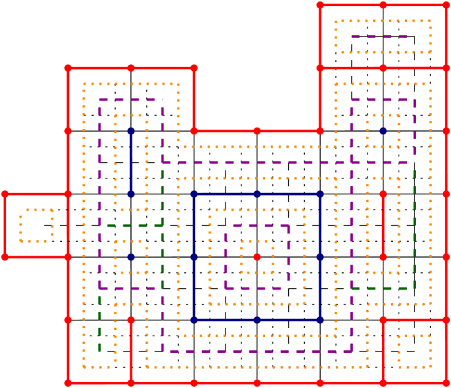
Figure 2.1. Ising and FK loops. Plain lines represent the domain $\mathcal{G}$, dashed lines represent $\mathcal{G}^{*}$ and dotted lines represent $\mathcal{G}^{b}$. In red and blue, the primal FK configuration $\omega$ ($k(\omega)=7$), red corresponding to FK connected components carrying $+$ Ising spins, and blue to FK components carrying $-$ spins. The green and purple represent the dual FK configuration, with purple being the subset traced by Ising loops. In orange, the set of FK loops.

We consider the usual square grid $\mathbb{Z}^{2}$, with the usual adjacency relation (denoted $\sim$). We denote by $\left(\mathbb{Z}^{2}\right)^{*}$ the dual graph, by $(\mathbb{Z}^{2})^{m}$ the medial graph (whose vertices are the centers of edges of $\mathbb{Z}^{2}$; two vertices of $(\mathbb{Z}^{2})^{m}$ are adjacent if the corresponding edges of $\mathbb{Z}^{2}$ share a vertex) and by $(\mathbb{Z}^{2})^{b}$ the bi-medial graph (i.e. the medial graph of $(\mathbb{Z}^{2})^{m}$). Note that $(\mathbb{Z}^{2})^{b}$ has a natural embedding in the plane as $\frac{1}{2}\mathbb{Z}^{2}+(\frac{1}{4},\frac{1}{4})$. In the following, we will be interested in particular finite subgraphs of $\mathbb{Z}^{2}$, namely those subgraphs that can be constructed as the collection of vertices and edges contained in a given simply-connected finite union of faces of $\mathbb{Z}^{2}$. We will refer to such finite subgraphs as discrete domains. For a discrete domain $\mathcal{G}$, we denote by $\mathcal{G}^{*}$ the dual of $\mathcal{G}$, by $\mathcal{G}^{m}$ the medial of $\mathcal{G}$ and by $\mathcal{G}^{b}$ the bi-medial of $\mathcal{G}$ (see Figure 2.1, in particular for how these are defined at the boundary). We denote by $\partial\mathcal{G}\subset\mathcal{G}$ the (inner) boundary of $\mathcal{G}$, which we either see as the set of vertices of $\mathcal{G}$ adjacent to $\mathbb{Z}^{2}\setminus\mathcal{G}$, or as the circuit of edges separating the faces of $\mathcal{G}$ from those of $\mathbb{Z}^{2}\setminus\mathcal{G}$.

Consider a Jordan domain $\Omega\subset\mathbb{C}$, i.e. such that its boundary $\partial\Omega$ is a simple closed curve. We call discretization of $\Omega$ a family $\left(\Omega_{\delta}\right)_{\delta}$ of discrete domains of $\delta\mathbb{Z}^{2}$ (the square grid of mesh size $\delta>0$) such that $\partial\Omega_{\delta}\to\partial\Omega$ (where we identify $\partial\Omega_{\delta}$ with its edge circuit) as $\delta\to 0$ in the topology of uniform convergence up to reparametrization. Note that any Jordan domain admits a discretization.

2.2. Ising Model

The Ising model (see e.g. [Gri06, FrVe17] for modern introductions) on a discrete domain $\mathcal{G}$ at inverse temperature $\beta>0$ consists of random configurations $\left(\sigma_{x}\right)_{x\in\mathcal{G}}$ of $\pm 1$ spins with probability proportional to $\exp\left(-\beta H\left(\sigma\right)\right)$ where the energy $H$ is given by $-H\left(\sigma\right)=\sum_{x\sim y}\sigma_{x}\sigma_{y}$ (the sum is over all pair of adjacent spins of $\mathcal{G}$). We will focus on the Ising model at the critical temperature, i.e. with $\beta=\beta_{c}$. If there are no particular conditions on the spins of $\partial\mathcal{G}$ we speak of free boundary conditions, if the spins of $\partial\mathcal{G}$ are conditioned to be $+1$ (resp. $-1$), we speak of $+$ boundary conditions (resp. $-$ boundary conditions).

2.3. FK Model

The Fortuin-Kasteleyn (FK) model (or random-cluster model, see [Gri06] for a background reference) on a discrete domain $\mathcal{G}$ is a (dependent) bond percolation model, which assigns a random open or closed state to the edges of $\mathcal{G}$. We then call configuration the set of the open edges of $\mathcal{G}$. The $\mathrm{FK}\left(p,q\right)$ model (with parameters $0\leq p\leq 1$, and $q\geq 1$ being a real number) assigns to a configuration $\omega$ a probability proportional to $p^{\mathbf{o}\left(\omega\right)}\left(1-p\right)^{\mathbf{c}\left(\omega\right)}q^{\mathbf{k}\left(\omega\right)}$, where $\mathbf{o}\left(\omega\right)$ is the number of open edges, $\mathbf{c}\left(\omega\right)$ the number of closed edges and $\mathbf{k}\left(\omega\right)$ the number of clusters of $\omega$, i.e. the number of connected components in the subgraph of $\mathcal{G}$ obtained by deleting all the closed edges. The above description defines what is called the FK model with free boundary conditions; the FK model with wired boundary conditions if obtained when conditioning all the boundary edges to be open (i.e. the edges between vertices of $\partial\mathcal{G}$ are forced open).

An important feature of the two-dimensional FK model is duality (see [Gri06, Section 6.1]). For an FK configuration $\omega$ on a discrete domain $\mathcal{G}$, we define the dual configuration $\omega^{*}$ on $\mathcal{G}^{*}$ whose open edges are the dual to the closed edges of $\omega$ and vice versa. It can be shown that for $p\left(1-p\right)^{-1}p^{*}\left(1-p^{*}\right)^{-1}=q$, the dual of an $\mathrm{FK}\left(p,q\right)$ configuration on $\mathcal{G}$ with wired boundary conditions is an $\mathrm{FK}\left(p^{*},q\right)$ configuration on $\mathcal{G}^{*}$ with free boundary conditions. The self-dual (or critical, see [BeDC12]) FK model corresponds to $\mathrm{FK}\left(p_{\mathrm{sd}},q\right)$, where the self-dual value $p_{\mathrm{sd}}=\frac{\sqrt{q}}{1+\sqrt{q}}$ is such that $p_{\mathrm{sd}}^{*}=p_{\mathrm{sd}}$.

2.4. FK-Ising Model

When $q=2$, the FK model is called the FK-Ising model. The Ising model at inverse temperature $\beta$ can be sampled from the FK-Ising model with $p=1-e^{-2\beta}$ by performing percolation on the FK clusters, see e.g. [Gri06, Section 2.3]: for each FK cluster we toss a balanced coin and assign the same $\pm 1$ spin value (depending on the tossed coin) to all the vertices of the cluster, and do this independently for each cluster. The self-dual FK-Ising model with $p_{\mathrm{sd}}=\frac{\sqrt{2}}{1+\sqrt{2}}$ corresponds to the critical Ising model. In this paper, the only FK model we will work with is the self-dual FK-Ising model. In order to clearly distinguish it from the Ising model, we will often refer to the self-dual FK-Ising model as just the FK model.

2.5. Ising Loops

A sequence of vertices $v_{1},\ldots,v_{n}$ is called a strong path if $v_{i}\sim v_{i+1}$ for $1\leq i<n$ (where $\sim$ denotes the adjacency relation) and a weak path if $v_{i}$ is weakly adjacent to $v_{i+1}$ (i.e. $v_{i}$ and $v_{i+1}$ share a face) for $1\leq i<n$.

Consider the Ising model on a discrete domain $\mathcal{G}\subset\mathbb{Z}^{2}$. An Ising loop is an oriented simple loop on $\mathcal{G}^{*}$ (i.e. a closed strong path of $\mathcal{G}^{*}$ such that no edge in the path is used twice) and such that any edge of the loop has a $+$ spin on its left and a $-$ spin on its right. In other words, an Ising loop separates a weak path of $+$ spins and a weak path of $-$ spins, and is hence clockwise-oriented if it has $+$ spins outside and $-$ spins inside (and counter-clockwise oriented otherwise). An Ising loop is called leftmost if it follows a strong path of $+$ on its left side, and rightmost if it follows a strong path of $-$ spins on its right.

In a domain carrying $+$ boundary conditions, an Ising loop is called outermost if it is not strictly contained inside another Ising loop, i.e. if it is not separated from the boundary by a a closed weak path of $-$ spins. Let us now define the level of an Ising loop (in a domain with $+$ boundary conditions). An Ising loop is said to be of level 1, if it is outermost, of level $2k$ for $k\geq 1$ if it is contained inside an Ising loop of level $2k-1$ and if it is not separated by a weak path of $+$ spins from that loop, and of level $2k+1$ for $k\geq 1$ if it is contained inside of an Ising loop of level $2k$ and if it is not separated by a weak path of $-$ spins from that loop. Note that two distinct outermost loops can intersect. However, the level of a loop is a well-defined integer: for example, there are not outermost loops of level $2$, as an outermost loop cannot be strictly contained in the interior of another Ising loop.

2.6. FK Loops and Cut-Out Domains

Given an FK configuration, the set of FK interfaces forms a set of loops on $\mathcal{G}^{b}$. A bi-medial edge is part of an FK interface if it lays between a primal FK cluster and a dual FK cluster, i.e. if it does not cross a primal open edge or a dual open edge. With wired or free boundary conditions, it is easy to see that the set of bi-medial edges that are part of an FK interface forms a collection of disjoint loops (in contrast to Ising loops, which may intersect).

The level of an FK loop is defined by declaring a loop of level 1 or outermost if it is not contained inside another FK loop, and of level $k>1$ if it is contained in the interior of exactly $k-1$ distinct FK loops. An FK loop of level $k>1$ is hence an outermost FK loop in the interior of an FK loop of level $k-1$. Note that, as FK loops are disjoint, the interior of two FK loops of same level $k$ are disjoint.

We call the interior of an outermost FK loop a cut-out domain. This notion will be crucial for us in the scaling limit. The set of FK loops satisfies the following spatial Markov property (see [Gri06, Theorem 3.4]): consider the FK model with wired boundary conditions, conditionally on the outermost FK loops, the model inside the cut-out domains consists of independent FK models with free boundary conditions.

Remark 2.

In the coupling with FK, the Ising loops are always a subset of the dual FK configuration. In particular Ising loops and FK loops never cross. As a consequence, all Ising loops are contained in the cut-out domains of the corresponding FK configuration.

2.7. The Space of Loop Collections

An oriented loop $\gamma$ is an equivalence class of continuous maps from the unit circle $\mathbb{S}^{1}$ to the plane $\mathbb{R}^{2}$, where the equivalence is given by orientation-preserving reparametrizations.

Consider the metric $d_{\Gamma}$ on the space of oriented loops defined as the supremum norm up to reparametrization: $d_{\Gamma}\left(\gamma,\tilde{\gamma}\right)=\inf\|\gamma-\tilde{\gamma}\|_{\infty}$, where the infimum is taken over all orientation-respecting parametrizations of the loops $\gamma$ and $\tilde{\gamma}$. We define the space $\Gamma$ to be the completion of the set of simple oriented loops for the metric $d_{\Gamma}$: $\Gamma$ is the set of oriented non-self-crossing loops (including trivial loops reduced to points).

The space $\mathcal{X}$ of loop collections is the space of at most countable collections $\left\{\gamma_{i}\right\}_{i\in I}$ of elements of $\Gamma$ (loops can appear with multiplicity, and we include the empty collection), such that

• For each $i\in I$, the loop $\gamma_{i}$ is not reduced to a point.

• For each scale $\varepsilon>0$, the set of indices $\left\{i\in I:\mathrm{diam}\left(\gamma_{i}\right)\geq\varepsilon\right\}$ is finite, where $\mathrm{diam}$ denotes the Euclidean diameter.

We now define a $\sigma$-algebra on $\mathcal{X}$. A matching of two sets $I$ and $J$ will denote a subset $\pi\subseteq I\times J$ such that for each $i\in I$ there is at most one $j\in J$ such that $(i,j)\in\pi$, and reciprocally, for each $j\in J$ there is at most one $i\in I$ such that $(i,j)\in\pi$. Given a matching $\pi$, we denote by $I^{\pi}$ (resp. $J^{\pi}$) the set of unmatched indices of $I$ (resp. $J$), i.e. the subset of indices $i\in I$ (resp. $j\in J$) such that for all $j\in J$ (resp. $i\in I$), $(i,j)\notin\pi$.

We work with the Borel $\sigma$-algebra on $\mathcal{X}$ associated to the following metric:

$$d_{\mathcal{X}}\left(\left\{\gamma_{i}\right\}_{i\in I},\left\{\gamma^{\prime}_{j}\right\}_{j\in J}\right)=\inf_{\pi}\max\left(\sup_{\left(i,j\right)\in\pi}d_{\Gamma}\left(\gamma_{i},\gamma^{\prime}_{j}\right),\sup_{i\in I^{\pi}}\mathrm{diam}\left(\gamma_{i}\right),\sup_{j\in J^{\pi}}\mathrm{diam}\left(\gamma^{\prime}_{j}\right)\right),$$

where the infimum is taken over all matchings $\pi$ of the index sets $I$ and $J$.

2.8. The Interior of a Non-Self-Crossing Loop

The following Lemma gives a number of useful facts about non-self-crossing loops

Lemma 3.

The connected components of the interior of a non-self-crossing loop are open sets homeomorphic to discs, whose boundaries can be traced by continuous curves.

We call these connected components cut-out domains. The boundary of a cut-out domain is a curve, which is not necessarily simple. We will make convergence statement about cut-out domains, these will always be for the topology of uniform convergence up to reparametrization for the boundary curves.

Proof.

Let us first give a formal definition of what it means for a connected component of the complement of a loop $\gamma$ to be in the interior of $\gamma$. Consider a continuous family of simple smooth curves $\gamma_{t}$ that converge to $\gamma$ when $t\rightarrow 0$. Without loss of generality, we can assume that all the curves $\gamma_{t}$ and $\gamma$ are positively oriented. Given a point $z$ in the complement of $\gamma_{t}$, the line integral

(2.1) $$I_{t}(z)=\frac{1}{2\pi i}\oint_{\gamma_{t}}\frac{1}{w-z}dw$$

takes the value $1$ or $0$ depending on whether the point $z$ is inside or outside $\gamma_{t}$. For any point $z\notin\gamma$, the quantity $I_{t}(z)$ is eventually well-defined (as $t\downarrow 0$), and as it is continuous in $t$, needs to be constant. We obtain a limiting value $I(z)=1\ {\rm or}\ 0$, defined off $\gamma$, and locally constant where defined, hence constant on the connected components of the complement of $\gamma$. We call such a component interior if $I=1$ on it, and exterior otherwise.

We now prove that connected components of the complement of a non-self-crossing loop $\gamma$ in the compactified plane $\widehat{\mathbb{R}^{2}}=\mathbb{S}^{2}$ are homeomorphic to open discs. Indeed, consider a sequence of simple loops $\gamma^{n}\rightarrow\gamma$, and a point $z\notin\gamma$. Let $D$ be the connected component of $\mathbb{S}^{2}\setminus\gamma$ containing $z$. Consider the uniformization map $\phi^{n}$ from the unit disk $\mathbb{D}$ to the connected component of $\mathbb{S}^{2}\setminus\gamma^{n}$ containing $z$, normalized so that $0$ is sent to $z$ and so that the derivative there is a positive real. These maps converges uniformly on compact subsets of the disc to a conformal map $\phi$ (by Caratheodory’s theorem [Pom92, Theorem 1.8]), and the image $\phi(\mathbb{D})=D$, is hence the image of a disk by a one-to-one bicontinuous map, so is itself an open set homeomorphic to the disk.

Finally, we show that the boundary of the cut-out domain $D$ containing $z$ can be traced by a continuous curve. We first show that, given another cut-out domain $D_{w}$ containing the point $w$, we can construct a subloop $\widetilde{\gamma}$ of $\gamma$ whose interior is a reunion of interior connected components of $\gamma$, that include $D$ but not $D_{w}$.

We consider an approximation by simple curves $\gamma^{n}\rightarrow\gamma$. For $n$ large enough, the points $z$ and $w$ are interior to $\gamma^{n}$. We call $\eta^{n}$ the infimum of the diameters of curves joining two points of $\gamma^{n}$ and otherwise staying in its interior that separate $z$ from $w$ in the interior of $\gamma^{n}$. We then pick such a curve, of diameter no more than $2\eta^{n}$ and call its boundary points $\gamma^{n}(u^{n})$ and $\gamma^{n}(v^{n})$. Up to extracting a subsequence, we can assume by compactness that $u^{n}\rightarrow u$ and $v^{n}\rightarrow v\neq u$. Note that $\eta^{n}\rightarrow 0$ as $z$ and $w$ belong to different connected components in the limit. Hence $\gamma(u)=\gamma(v)$ is a double point of the curve, and moreover, by construction, the two corresponding subloops of $\gamma$, say $\gamma_{1}$ and $\gamma_{2}$, are positively oriented, non-self-crossing, and do not cross each other. By looking at the integral formula (2.1) to determine whether a point is surrounded by a loop, and using that $I^{\gamma}=I^{\gamma_{1}}+I^{\gamma_{2}}$, we see that each interior cut-out domain of $\gamma$ is either in the interior of $\gamma_{1}$ or in the interior of $\gamma_{2}$. Moreover it is clear that one of these loops, say $\gamma_{1}$, surrounds $D_{w}$, and the other, $D$. This provides the subloop $\widetilde{\gamma}=\gamma_{2}$ as claimed.

Enumerating the interior cut-out domains of $\gamma$ using points they contain $z,w_{1},w_{2},\cdots,w_{l},\cdots$, we can iteratively extract subloops $\gamma^{l}$ of $\gamma$ that contain $D$ in their interior but not $D_{w_{1}},\cdots,D_{w_{l}}$. The curves $\gamma^{l}$ converge up to reparametrization (at the very least it is easy to see that we can assume convergence up to extracting a subsequence). The limiting loop $\gamma_{D}$ is by construction a positively oriented non-self-crossing loop whose interior is $D$. ∎

2.9. Nested and Non-Nested Loop Collections

We say that two loops $\gamma$ and $\gamma^{\prime}$ of $\Gamma$ do not cross each other if we can find two sequences $(\gamma_{n})_{n\in\mathbb{N}}$ and $(\gamma^{\prime}_{n})_{n\in\mathbb{N}}$ of elements of $\Gamma$ such that $\gamma_{n}\rightarrow\gamma$, $\gamma^{\prime}_{n}\rightarrow\gamma^{\prime}$, and for each $n\in\mathbb{N}$, the loops $\gamma_{n}$ and $\gamma^{\prime}_{n}$ are disjoint.

Lemma 4.

Given two distinct non-self-crossing loop that do not cross each other, then either

• their interiors are disjoint, or

• the interior of one of the loops, say $\gamma$, is included in the interior of the other loop $\gamma^{\prime}$.

In the second case, we say that the loop $\gamma$ is nested in $\gamma^{\prime}$.

Proof.

We omit the proof of this simple result, which can formally be proven using (2.1). ∎

A non-crossing collection of loops is a loop collection of $\mathcal{X}$ such that no two loops cross each other. A non-nested collection of loops is a loop collection of $\mathcal{X}$ that is non-crossing and such that no loop is nested in another.

Given a non-crossing loop collection such that no two loops are equal, we define the level of a loop as the number of loops containing it, plus $1$. Note that the level of a loop is always finite, by the diameter constraint on loop collections. Outermost loops are loops of level 1, or alternatively, loops that are not nested in any other loop. Similarly, innermost loops are loops such that no other loop is nested inside of them. Given a non-crossing collection of loops $\mathcal{C}$, we call cut-out domains of $\mathcal{C}$ the cut-out domains of the innermost loops of $\mathcal{C}$.

This general definition for the level of a loop does not apply to discrete Ising loops (which is not a non-crossing collection, see Section 2.5), but coincides with the definitions we give for discrete FK loops in Section 2.6.

2.10. Measurability of Some Loop Collections

Lemma 5.

The space $\mathcal{X}$ is complete and separable, hence is a Polish space. Moreover, the following events on $\mathcal{X}$ are measurable for the Borel $\sigma$-algebra:

• The collection $\left(\gamma_{i}\right)_{i\in I}$ is non-crossing.

• The collection $\left(\gamma_{i}\right)_{i\in I}$ is non-nested.

• The loops of the collection $\left(\gamma_{i}\right)_{i\in I}$ are disjoint.

• All the loops of $\left(\gamma_{i}\right)_{i\in I}$ are simple.

Proof.

The set of finite collections of simple loops made of edges of one of the lattices $2^{-n}\mathbb{Z}^{2}$ forms a countable family which is dense in $\mathcal{X}$. In other words, $\mathcal{X}$ is separable.

We now show that $\mathcal{X}$ is complete. Let $\mathcal{C}_{n}$ be a Cauchy sequence in $\mathcal{X}$. Let us call $N_{n}(\varepsilon)$ the number of loops of $\mathcal{C}_{n}$ that are of diameter larger than or equal to $\varepsilon$. $N_{n}$ is a non-increasing integer-valued left-continuous function that goes to $0$ as $\varepsilon$ goes to $\infty$. From this, we can see that $N_{n}(\varepsilon)$ converges pointwise to a function $N$ as $n\to\infty$, except maybe at the jump points (i.e., discontinuity points) of the limiting function $N$. Let us consider a sequence of sizes $\varepsilon_{i}\to 0$ whose elements are distinct from the jump points of $N$. For a fixed $\varepsilon_{i}$, for any $n,m$ large enough (say $n,m\geq n_{0}$), the collections $\mathcal{C}_{n}$ and $\mathcal{C}_{m}$ will have the same number of loops of diameter larger than $\varepsilon_{i}$. Moreover, provided that $n,m$ are large enough, any matching between the loops of $\mathcal{C}_{n}$ and $\mathcal{C}_{m}$ that is close to providing the optimal matching distance $d_{\mathcal{X}}(\mathcal{C}_{n},\mathcal{C}_{m})$ will have to match all of the loops of diameter larger than $\varepsilon_{i}$ with each other. From this, we see that we can match consistently (for all $n\geq n_{0}$) the $N(\varepsilon_{i})$ large loops in such a way that their $d_{\Gamma}$ distance goes uniformly to $0$. The fact that the space $\mathcal{X}$ is complete hence follows from the fact that $\Gamma$ is.

A number of sets of loop collections can then be shown to me measurable:

• The set of collections that consists of non-crossing loops is a closed set of $\mathcal{X}$, hence is measurable. The same holds for non-nested collections.

• For each $\varepsilon,\delta>0$, let us consider the set of collections $D_{\varepsilon,\delta}$ such that the open $\delta$-neighborhoods of all the loops of diameter strictly larger than $\varepsilon$ are all disjoint. The set $D_{\varepsilon,\delta}$ is closed, and we can write the set $D$ of collections such that all loops are disjoint as $D=\cap_{\epsilon}\cup_{\delta}D_{\varepsilon,\delta}$. Hence $D$ is a measurable set.

• We say that a loop $\gamma$ is in the set $\Sigma_{\delta}$ of approximately simple loops at scale $\delta$ if any of its double points cuts up the loop $\gamma$ in two pieces that are not both of diameter larger than or equal to $\delta$. Note that $\Sigma_{\delta}$ is an open set. For each $\varepsilon,\delta>0$, let us consider the set of collections $S_{\varepsilon,\delta}$ such that all the loops of diameter larger than or equal to $\varepsilon$ belong to $\Sigma_{\delta}$. The set is $S_{\varepsilon,\delta}$ is open, and we can write the set $S$ of collections such that all loops are simple as $S=\cap_{\epsilon}\cap_{\delta}S_{\varepsilon,\delta}$. Hence $S$ is a measurable set.

∎

2.11. Conformal Loop Ensembles

The CLE measures have been introduced in [She09] as the natural candidates to describe conformally invariant collections of loops arising as scaling limits of statistical mechanics interfaces. They form a family indexed by $\kappa\in(\frac{8}{3},8]$ of random collections of $\mathrm{SLE}_{\kappa}$-like loops.

The usual $\mathrm{CLE}_{\kappa}$ measure (as opposed to nested $\mathrm{CLE}_{\kappa}$, defined below) is defined on a planar simply-connected domain and consists of a collection of non-nested loops. For $\kappa\in(\frac{8}{3},4]$, the usual $\mathrm{CLE}_{\kappa}$ have an elegant loop-soup construction [ShWe12, Theorem 1.6]: the $\mathrm{CLE}_{\kappa}$ loops can be constructed by taking the outer boundaries of clusters of loops in a Brownian loop soup of intensity $c=\left(3\kappa-8\right)\left(6-\kappa\right)/2\kappa$.

We now iteratively define a random loop collection called nested $\mathrm{CLE}_{\kappa}$. Its outermost loop (or level $1$) have the law of a usual $\mathrm{CLE}_{\kappa}$. Given its loops of level $k\geq 1$, we define its loops of level $k+1$ as independent samples of usual $\mathrm{CLE}_{\kappa}$ in each of the cut-out domains associated to the loops of the level $k$. We choose to orient CLE loops according to their level: clockwise for odd level loops, and counterclockwise for even level loops.

2.12. CLE Markovian Characterization

An important result on CLEs is their Markovian characterization.

Theorem ([ShWe12, Theorem 1.4 and Section 2.1]).

A family of measures $\mu_{\Omega}$ on non-nested collections of simple loops defined on simply-connected domains $\Omega$ is the usual $\mathrm{CLE}_{\kappa}$ for a certain $\kappa\in(\frac{8}{3},4]$ if and only if the following holds with probability $1$:

• The collection is locally finite: for any $\varepsilon>0$ and any bounded region $K\subseteq\Omega$, there are only finitely-many loops of diameter greater than $\varepsilon$ in $K$.

• Distinct loops of the collection are disjoint.

• The family is conformally invariant: for any conformal mapping $\varphi:\Omega\to\varphi\left(\Omega\right)$, we have $\varphi_{\ast}\mu_{\Omega}=\mu_{\varphi\left(\Omega\right)}$.

• The family satisfies the Markovian restriction property on any simply-connected domain $\Omega$: for any compact set $K\subset\Omega$ such that $\Omega\setminus K$ is simply-connected, if $\left\{\gamma_{i}\right\}_{i\in I}$ is sampled from $\mu_{\Omega}$, setting $I_{K}:=\left\{i:\gamma_{i}\cap K\neq\emptyset\right\}$ we have that $\left\{\gamma_{i}\right\}_{i\in I}$ conditioned on $\left\{\gamma_{i}\right\}_{i\in I_{K}}$ has the law of $\mu_{\Omega\setminus\mathcal{L}_{K}}$, where $\mu_{\Omega\setminus\mathcal{L}_{K}}$ is defined as the independent product of $\mu_{\Omega^{\prime}}$ taken over all connected components $\Omega^{\prime}$ of $\Omega\setminus\mathcal{L}_{K}$ and where $\mathcal{L}_{K}=K\cup\left\{\mathrm{Inside}\left(\gamma_{i}\right)\cup\gamma_{i}:i\in I_{K}\right\}$.

3. Main Theorem

3.1. Statement and Strategy

Let us now give the precise version of our main result:

Theorem 6.

Consider the critical Ising model with $+$ boundary conditions on a discretization $\left(\Omega_{\delta}\right)_{\delta>0}$ of a Jordan domain $\Omega$,. Then as the mesh size $\delta\to 0$, the set of all leftmost Ising loops converges in law with respect to $d_{\mathcal{X}}$ to the nested $\mathrm{CLE}_{3}$.

Furthermore, for any $\varepsilon>0$, the following holds with probability tending to $1$ as $\delta\to 0$: for any Ising loop $\ell$ of diameter larger than $\varepsilon$, there exists a leftmost loop $\ell_{L}$ such that $d_{\Gamma}(\ell,\ell^{L})\leq\varepsilon$ and such that the connected components of $\left(\ell\cup\ell^{L}\right)\setminus\left(\ell\cap\ell^{L}\right)$ have diameter less than $\varepsilon$.

The second part of the statement (that will be proved as Lemma 14) tells us that in order to understand all Ising loops, it is enough to understand leftmost Ising loops. Indeed, any macroscopic Ising loop $\ell$ is close to a leftmost loop $\ell_{L}$ in a very strong sense: not only are the loops close in the topology of uniform distance up to reparametrization, but the edges they share form a dense subset of each loop.

Remark 7.

The same result holds for rightmost loops, as the proof will show.

The strategy for the proof, illustrated in Figure 3.1, is the following:

• We first prove that the collection of level one (i.e. outermost) Ising loops has a conformally invariant scaling limit (Section 5).

• We then show that this limit consists of loops that are simple, do not touch the boundary or each other, and satisfy the Markovian restriction property (Section 6.1).

• We then use the characterization of CLE to identify the scaling limit of the outermost loops as non-nested $\mathrm{CLE}_{3}$ and finally obtain the convergence of all Ising loops to nested $\mathrm{CLE}_{3}$ (Section 6.2).

Remark 8.

In [MSW16], the authors explain how $\mathrm{CLE}_{3}$ can be obtained by performing a percolation on the $\mathrm{CLE}_{16/3}$ clusters (a procedure analogous to the one used in the discrete to construct the Ising model from the FK model). This approach explains how the joint coupling works in the continuum and provides a proof scheme for the joint convergence of Ising and FK loops towards a coupling of CLE_16/3 and CLE₃ (our approach does not, as we keep resampling the coupled FK model to further explore Ising loops). Remark 23 provides some of the technical tools needed for this joint convergence, but some further study of the set of discrete FK loops seems needed in order to get a complete argument.

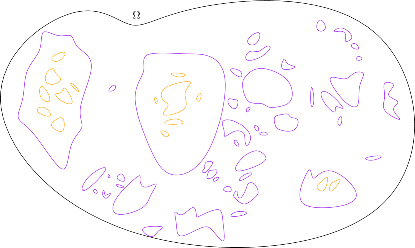
(a) The Ising loops to explore (colors for Ising loops: level 1 in purple, level 2 in orange)

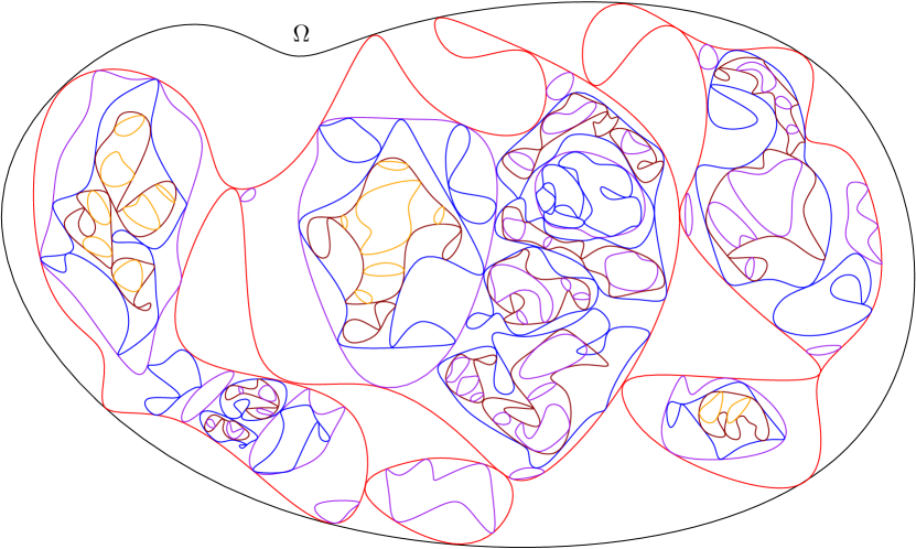
(b) Ising loops and the coupled FK (colors for FK loops: level 1 in red, level 2 in blue, level 3 in brown)

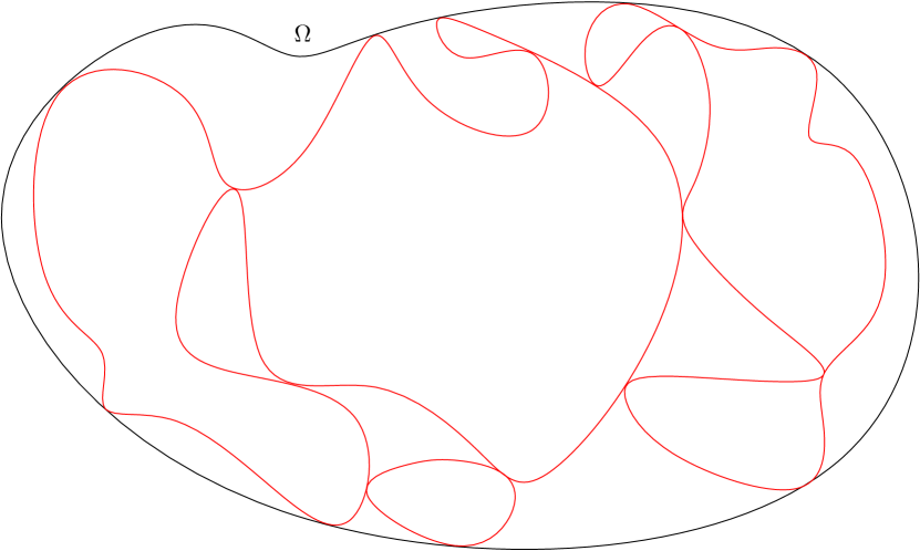
(c) We first consider all FK loops of level 1

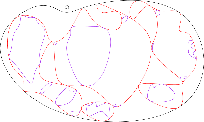
(d) Then, we find all Ising loops (of level 1) that touch the explored FK loops

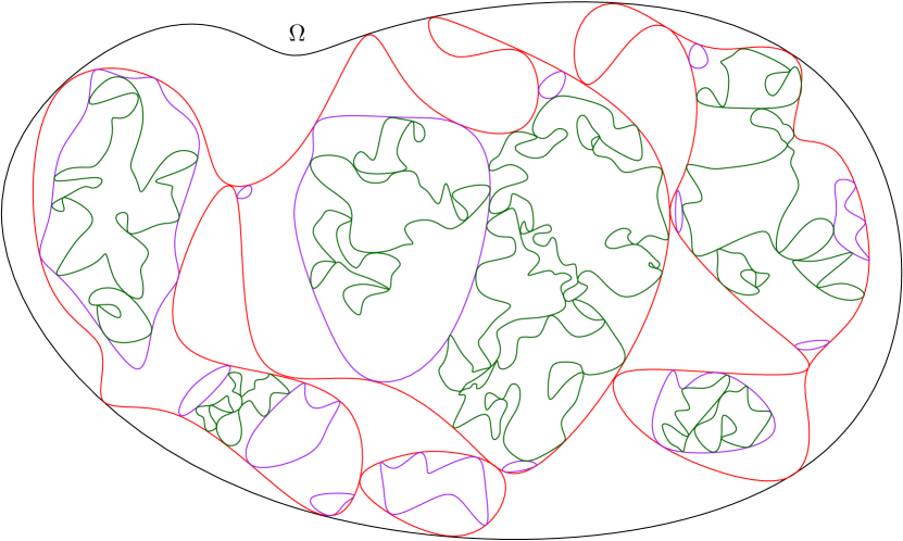
(e) We resample the FK loops (in green) in the domains bounded by the Ising loops we have found

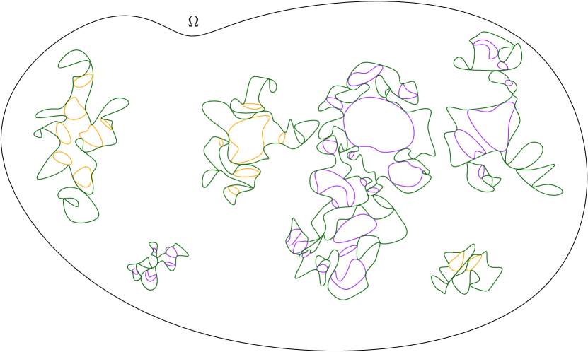
(f) We find all Ising loops (of level 1 and 2) that touch the resampled outermost FK loops

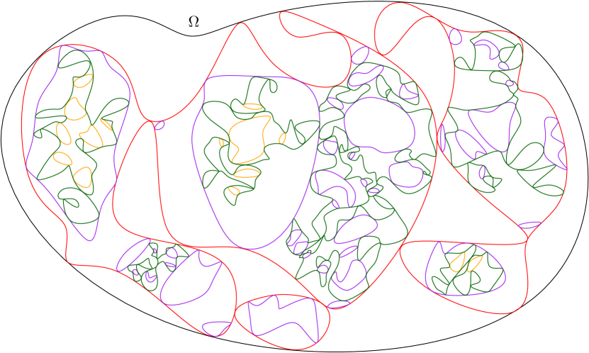
(g) All the loops used in the exploration process

Figure 3.1. The exploration scheme

4. Scaling Limits of Ising and FK Interfaces

In this section, we state two results on which our proof relies: first, the identification of the scaling limit of the free boundary conditions arc for the Ising model and second, the conformal invariance of the scaling limit of the FK interface loops.

4.1. Ising Free Arc Ensembles

The first result that we need is the identification of the scaling limit of the Ising arcs that arise with free boundary conditions. For the Ising model on a discrete domain $\mathcal{G}$ with free boundary conditions, we call an Ising arc a spin interface that links two boundary points. In the continuous, we refer to the set of arcs produced by a branching SLE${}_{3}(-\frac{3}{2},-\frac{3}{2})$ as the Free Arc Ensemble (FAE) [BDH16].

Theorem 9 ([BDH16, Theorem 6]).

Consider the critical Ising model on a discretization $\left(\Omega_{\delta}\right)_{\delta>0}$ of a Jordan domain $\Omega$, with free boundary conditions. Then as $\delta\to 0$, the set of all Ising arcs converges in law to the Free Arc Ensemble (for the Hausdorff metric on sets of curves, where curves are equipped with the topology of uniform convergence up to reparametrization).

As explained in [BDH16], the scaling limits of the interfaces linking pairs of boundary points, and hence boundary touching loops, can be deterministically recovered by gluing the FAE arcs. These two sets of curves (the arcs on the one hand and the scaling limit of the boundary touching loops) contain the same data in the continuous.

Let us describe how boundary touching loops can be recovered from Ising arcs. We formally put $+$ spins on the boundary of a discrete domain $\mathcal{G}$ and consider the free Ising model inside of $\mathcal{G}$: the formal boundary spins do not interact, but they play a role in determining what we call an Ising interface. Given a spin configuration $\sigma$, we will consider the spin-flip of $\sigma$ which is the spin configuration obtained by switching the value of all the spins inside of $\mathcal{G}$, except for the formal boundary spins that stay at their fixed $+$ value.

Given a face $z\in\mathcal{G}$ and an edge $b$ on the boundary of $\mathcal{G}$ (i.e., an edge that lies between a fixed $+$ spin and a free spin), let $\mathcal{A}(z,b)$ be the set of all the leftmost Ising arcs (i.e., leftmost Ising interfaces joining two points of the boundary of $\mathcal{G}$) that separate $z$ from $b$ in $\mathcal{G}$. The proximity to $z$ gives a natural ordering of the set $\mathcal{A}(z,b)$: given two distinct arcs of $\mathcal{A}(z,b)$, one of them is always closer to $z$, in the sense that it separates the other arc from $z$. When the set $\mathcal{A}(z,b)$ is non-empty, we define $a(z,b)$ to be the arc closest to $z$ among all elements of this set, otherwise, we let $a(z,b)=b$. We call the inside (resp. the outside) of $a(z,b)$ the set of spins neighboring the arc $a(z,b)$ on the side of $z$ (resp. on the side of $b$).

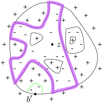
Figure 4.1. The arcs and loops of an Ising configuration in $\mathcal{G}$. The path outlined in purple is the concatenation of the arcs $a(z,b)$ over all the boundary edges $b$, as in Lemma 10. The green arc belongs to $\mathcal{A}(z,b^{\prime})$ but is not the arc $a(z,b^{\prime})$ .

We now explain how to recover from the Ising arcs the set $\mathcal{L}\left(\mathcal{G}\right)$ of all the leftmost Ising loops that touch the boundary of $\mathcal{G}$ (see also Figure 5.1). Note that this construction relies on the formal $+$ spins on the boundary of $\mathcal{G}$.

Lemma 10.

For any spin configuration $\sigma$ and any face $z\in\mathcal{G}$, denoting by $\ell$ the concatenation of the arcs $a(z,b)$ over all the boundary edges $b$ (see Figure 4.1), we have

• Either, for any boundary edge $b$, the inside of $a(z,b)$ consists of $-$ spins only. In that case $\ell$ is a loop in $\mathcal{L}\left(\mathcal{G}\right)$.

• Or, for any boundary edge $b$, the inside of $a(z,b)$ consists of $+$ spins only. In that case, $\ell$ bounds a connected component $R$ of

  $$\widetilde{\mathcal{G}}=\mathcal{G}\setminus\bigcup_{\gamma\in\mathcal{L}(\mathcal{G})}\gamma$$

  that is not surrounded by a loop in $\mathcal{L}(\mathcal{G})$. Moreover, $\ell$ is an Ising loop for the spin-flipped configuration.

Proof.

Let us fix $z\in\mathcal{G}$, and assume that there exists an edge $b^{\prime}$ such that $a(z,b^{\prime})$ carries $-$ spins on its inside. Then the (weak) connected component $\mathcal{G}^{\prime}$ of $-$ spins attached to the arc $a(z,b^{\prime})$ disconnects $z$ from the boundary (as the arc $a(z,b^{\prime})$ is extremal). Hence the outer boundary of $\mathcal{G}^{\prime}$ consists of the arcs $a(z,b)$ where $b$ ranges over all boundary edges, which forces these arcs have to carry $-$ spins on their inside.

If the face $z$ is such that the above assumption does not hold, then all the edges of $a(z,b)$ carry $+$ spins on their inside. It is straightforward that their concatenation bounds a connected component $R$ of $\widetilde{\mathcal{G}}$ that is not surrounded by a loop in $\mathcal{L}(\mathcal{G})$. Note that given an edge $b$ such that the set $\mathcal{A}(z,b)$ is non-empty, the arc $a(z,b)$ carry $-$ spins on its outside and $+$ spins on its inside, whereas if $\mathcal{A}(z,b)$ is empty, $a(z,b)=b$ is a boundary edge lying between two $+$ spins. If we flip all the spins in the interior of $\mathcal{G}$, any edge of the boundary of $R$ will carry $-$ spins on its inside and $+$ spins on its outside. In other words the boundary of the region $R$ is an Ising loop for the spin-flipped configuration. ∎

4.2. Conformal Invariance of FK-Ising Interfaces and Cut-Out Domains

For the proof of our main theorem, we need the following result, which is closely related to (but independent of) the result of Kemppainen and Smirnov about the scaling limit of the boundary-touching FK loops in smooth domains [KeSm15]. This result includes in particular the convergence of FK cut-out domains to continuous cut-out domains, defined as the maximal domains contained inside the scaling limit of FK loops.

Proposition 11.

Consider the critical FK-Ising loops on a discretization $\left(\Omega_{\delta}\right)_{\delta}$ of a Jordan domain $\Omega$, with wired boundary conditions. The FK loops have a conformally invariant scaling limit (in law, with respect to $d_{\mathcal{X}}$) as the mesh size $\delta\to 0$. This scaling limit is almost surely a non-crossing collection. Furthermore the discrete cut-out domains of level one FK loops converge to the cut-out domains of the outermost loops of this scaling limit.

Proof.

The first part is proven as Proposition 22 in the Appendix and the second part follows from Remark 23 just after. ∎

5. Scaling Limit of Ising Outermost Loops

We start with a technical lemma to control the diameters of Ising loops: we show it is impossible to find an arbitrarily large collection of macroscopic Ising loops.

Given a collection $\mathcal{C}$ of loops, let $\underline{d}_{\mathcal{C}}$ (resp. $\overline{d}_{\mathcal{C}}$) denote the infimum (resp. supremum) of the diameters of the loops in $\mathcal{C}$. Consider the critical Ising model with $+$ boundary conditions on a discretization $\left(\Omega_{\delta}\right)_{\delta>0}$ of a Jordan domain $\Omega$. For any integer $n\geq 1$, we let $\underline{d}_{n}$ denote the supremum of the quantities $\underline{d}_{\mathcal{C}}$, where $\mathcal{C}$ ranges over all collections of $n$ disjoint Ising loops.

Lemma 12.

The quantity $\underline{d}_{n}$ converges in probability to $0$ as $n\to\infty$, uniformly in the mesh size $\delta$:

$$\forall\varepsilon_{1},\varepsilon_{2}>0,\ \exists n_{0}\in\mathbb{N},\ \forall\delta>0,\ \forall n\geq n_{0},\ \mathbb{P}\left[\underline{d}_{n}\geq\varepsilon_{1}\right]\leq\varepsilon_{2}.$$

Proof.

By contradiction, if this were not to the case, we could find $\varepsilon_{1},\varepsilon_{2}>0$ such that for any integer $n$, we could find a mesh size $\delta_{n}$ such, with probability at least $\varepsilon_{2}$, that there would be a collection $\mathcal{C}$ of $n$ disjoint Ising loops such that $\underline{d}_{\mathcal{C}}>\varepsilon_{1}$. Note that $\delta_{n}\to 0$ as, for each fixed $\delta$, one can draw only finitely many simple loops on the graph $\Omega_{\delta}$.

Given any scale $\eta<\varepsilon_{1}$, we can find a finite collection of annuli of inner radius $\eta$ and outer radius $\varepsilon_{1}$ such that the domain $\Omega$ is covered by the balls of radius $\eta$ at the center of these annuli. Moreover, we can pick such a covering collection by using a number $C\eta^{-2}$ of annuli, where $C$ is a constant that depends on the domain $\Omega$ but not on $\eta$. Each Ising loop has to intersect the inside of at least one of these annuli (as they form a cover of our domain), and so each Ising loop of diameter larger than $\varepsilon_{1}$ forces the existence of an Ising interface crossing in at least one of these annuli. In turn, the existence of more than $C\eta^{-2}(N-1)+1$ disjoint Ising loops of diameter larger than $\varepsilon_{1}$ implies that one of the annulus in the cover contains at least $N$ disjoint Ising interface crossings.

As Ising interfaces form a subset of the FK dual configuration through the Edwards-Sokal coupling, FK dual paths provide similar crossings: for any integer $N$, for any scale $\eta<\varepsilon_{1}$, we can find a mesh size $\delta<\eta$ such that with probability at least $\varepsilon_{2}$, there exists an annulus of inner radius $\eta$ and outer radius $\varepsilon_{1}$ which is crossed by $N$ disjoint dual FK arms.

However [CDH16, Lemma 5.7] (via the use of quasi-multiplicativity [CDH16, Theorem 1.3] to compute arm exponents) implies that FK $N$-arm monochromatic (i.e., all arms are primal or all arms are dual) exponents are larger than $2$ for $N$ large enough (note that, as FK measures are positively correlated, these exponents also provide upper bounds on dual crossing of annuli that intersect the wired boundary of our domain $\Omega$). Hence we can find an integer $N$, such that, provided that the scale $\eta$ is small enough, the probability that at least one annuli among $C\eta^{-2}$ is crossed by $N$ disjoint dual FK arms is arbitrarily small, uniformly in the mesh size $\delta$. This yields a contradiction, and so the quantity $\underline{d}_{n}$ converges to $0$ as claimed. ∎

Let us now argue that the outermost Ising loops have a conformally invariant scaling limit. Consider the critical Ising model with $+$ boundary conditions coupled with an FK model with wired boundary conditions on a discretization $\left(\Omega_{\delta}\right)_{\delta>0}$ of a Jordan domain $\Omega$.

Lemma 13.

As the mesh size $\delta\to 0$, the leftmost level one Ising loops converge in law with respect to the topology generated by $d_{\mathcal{X}}$ to a conformally invariant scaling limit.

Furthermore, in the scaling limit, the Ising loops are contained in the cut-out domains of the outermost FK loops.

Proof.

We are going to describe the collection $\mathcal{L}$ of leftmost level one Ising loops iteratively as a countable union of loop collections $\mathcal{L}=\cup_{n}\mathcal{L}_{n}$. Convergence will follow from the a.s. convergence of each of the loop collections $\mathcal{L}_{n}$, as well as from the fact that the supremum of the diameter of the loops in $\mathcal{L}_{n}$ goes to $0$ in probability as $n\to\infty$, uniformly in $\delta$.

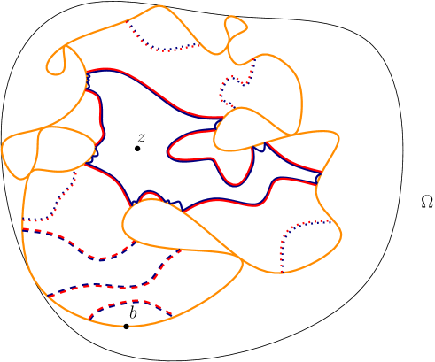
Figure 5.1. In orange, an FK loop touching the boundary of the domain $\Omega$: the corresponding primal FK cluster carries $+$ spins. In red and blue, paths of Ising $+$ and $-$ spins respectively. The plain paths correspond to the collection of arcs $a(z,b)$, that together draw an Ising loop of level 1 surrounding $z$. In dashed, a few arcs belonging to $\mathcal{A}(z,b)$.

Let us first describe $\mathcal{L}_{1}$ (see Figure 5.1). We start by conditioning on the outermost FK loops in $\Omega_{\delta}$. Let us denote by $\mathcal{C}_{1}$ the associated set of discrete cut-out domains in $\Omega_{\delta}$ (see Section 2.9). Any cut-out domain $C_{\delta}\in\mathcal{C}_{1}$ satisfies the following: it is bordered on its outside by a strong path of $+$ and, conditionally on $C_{\delta}$, the Ising spins inside of $C_{\delta}$ have free boundary conditions. Let us call $\mathcal{L}\left(C_{\delta}\right)$ the set of leftmost Ising loops in $C_{\delta}$ that touch the boundary of $C_{\delta}$ (note that we are in the setup of Lemma 10).

Now, consider the loop collection

$$\mathcal{L}_{1}=\bigcup_{C_{\delta}\in\mathcal{C}_{1}}\mathcal{L}\left(C_{\delta}\right),$$

where the union is over all cut-out domains $C_{\delta}\in\mathcal{C}_{1}$. We can pass the construction of $\mathcal{L}_{1}$ to the scaling limit. By Proposition 11, the discrete cut-out domains $C_{\delta}\in\mathcal{C}_{1}$ converge to the continuous cut-out domains as $\delta\to 0$. Moreover, for any cut-out domain $C=\lim C_{\delta}$, the Ising arc ensemble in $C_{\delta}$ converges to the (conformally invariant) Free Arc Ensemble in $C$ as $\delta\to 0$ (Theorem 9). Hence, the boundary touching loops $\mathcal{L}\left(C_{\delta}\right)$ converge (via the correspondence between arcs and loops explained in Lemma 10). Consequently, the collection $\mathcal{L}_{1}$ has a conformally invariant scaling limit.

Recall now that any Ising loop is contained inside one of the cut-out domains $C_{\delta}\in\mathcal{C}_{1}$ (Remark 2). For such a cut-out domain $C_{\delta}$, we have that the loops of $\mathcal{L}_{1}$ further cut $C_{\delta}$ in regions of two types (this is the dichotomy of Lemma 10):

• The regions enclosed by the loops of $\mathcal{L}_{1}$ (each loop in $\mathcal{L}_{1}$ separates an inner weak circuit of $-$ on its inside and a strong circuit of $+$ on its outside).

• The regions that are outside the loops of $\mathcal{L}_{1}$ (these regions have strong $+$ boundary conditions). Let us denote by $\mathcal{R}\left(C_{\delta}\right)$ the set of these regions.

A loop $\ell_{\delta}$ that is inside of $C_{\delta}$ hence falls into one of three categories:

• The loop $\ell_{\delta}$ is strictly contained inside of a loop of $\mathcal{L}_{1}$: in this case, it is of level two or higher (i.e. it is not outermost).

• The loop $\ell_{\delta}$ is contained inside of a loop $L_{\delta}\in\mathcal{L}_{1}$ and it shares an edge with $L_{\delta}$ (and hence is of level one, but not leftmost if it is distinct from $L_{\delta}$). The structure of these loops is described in Lemma 14 below.

• The loop $\ell_{\delta}$ is strictly contained in one of the regions in $\mathcal{R}\left(C_{\delta}\right)$.

In order to find the remaining leftmost level 1 Ising loops (i.e., the collection $\mathcal{L}\setminus\mathcal{L}_{1}$) we hence just need to look inside the regions in $\mathcal{R}\left(C_{\delta}\right)$.

Let us call

$$\mathcal{R}_{2}=\bigcup_{C_{\delta}\in\mathcal{C}_{1}}\mathcal{R}\left(C_{\delta}\right).$$

Any region $C_{\delta}\in\mathcal{R}_{2}$ carries strong $+$ boundary conditions, and its boundary is connected by a strong path of $+$ to the boundary of $\Omega_{\delta}$, so any leftmost level 1 Ising loop in $C_{\delta}$ is also a leftmost level 1 Ising loop of $\Omega_{\delta}$.

By resampling an FK representation with wired boundary conditions of the Ising model in each of the domains $C_{\delta}$, we can take the construction we just did for the unique region of $\mathcal{R}_{1}=\{\Omega_{\delta}\}$ (that yielded the loop collections $\mathcal{L}_{1}$) and apply this construction to each of the regions in $\mathcal{R}_{2}$. In particular, we construct a collection $\mathcal{C}_{2}$ of cut-out domains associated to the outermost FK loops in each region in $\mathcal{R}_{2}$, and use these to obtain a collection of leftmost level 1 Ising loops $\mathcal{L}_{2}$, as well as a set of smaller regions $\mathcal{R}_{3}$ with $+$ boundary conditions, that contain all the leftmost level 1 Ising loops that were neither in $\mathcal{L}_{1}$ nor in $\mathcal{L}_{2}$. We further iterate until all loops are found, so that $\mathcal{L}=\cup_{n}\mathcal{L}_{n}$. For each fixed $n$, the loop collection $\mathcal{L}_{n}$ has a conformally invariant scaling limit, for the same reason that $\mathcal{L}_{1}$ has.

To deduce the convergence of $\mathcal{L}=\cup_{n}\mathcal{L}_{n}$ from the convergence of the terms $\mathcal{L}_{n}$, we need them to uniformly converge in some sense: we will show that macroscopic Ising loops cannot belong to $\mathcal{L}_{n}$ for $n$ arbitrarily large. More precisely, we will now show that the quantity $\overline{d}_{\mathcal{L}_{n}}$ (the diameter of the largest loop in $\mathcal{L}_{n}$) tends to $0$ in probability as $n\to\infty$, uniformly in $\delta$. As the loops of $\mathcal{L}_{n}$ are contained in the domains belonging to $\mathcal{R}_{n}$, it is enough to show that the supremum $\overline{d}_{\mathcal{R}_{n}}$ of the diameters of the elements of $\mathcal{R}_{n}$ goes to $0$ in probability as $n\to\infty$, uniformly in $\delta$.

We now fix an integer $n\geq 1$, and consider an integer $1\leq i\leq n+1$. We denote by $\mathcal{S}_{i}$ the set of collections of $n$ disjoint loops $\ell_{1},\cdots,\ell_{n}$ such that

• For $1\leq j<i$, $\ell_{j}$ is the boundary of a domain in $\mathcal{R}_{j+1}$.

• For $i\leq j\leq n$, $\ell_{j}$ is an Ising loop.

• For any $1\leq j<n$, $\ell_{j+1}$ is contained in the interior of $\ell_{j}$.

For $1\leq i\leq n$, consider the following operation $F_{i}$ on spin configurations: condition first on the cut-out domains $\mathcal{C}_{i}$, and flip the Ising spins inside these domains. Conditioned on the cut-out domains $\mathcal{C}_{i}$, the Ising model inside of them has the law of independent Ising models with free boundary conditions. Hence the map $F_{i}$ is measure-preserving. Moreover the boundary of any domain in $\mathcal{R}_{i+1}$ becomes an Ising loop after the spin flip (by Lemma 10). Hence, any collection in $\mathcal{S}_{i+1}$ for the configuration $\sigma$ belongs to the set $\mathcal{S}_{i}$ for the configuration $F_{i}(\sigma)$. This gives the following estimate, for any $\varepsilon_{1}>0$:

$$\mathbb{P}\left[\sup_{\mathcal{C}\in\mathcal{S}_{i+1}}\underline{d}_{\mathcal{C}}\geq\varepsilon_{1}\right]\leq\mathbb{P}\left[\sup_{\mathcal{C}\in\mathcal{S}_{i}}\underline{d}_{\mathcal{C}}\geq\varepsilon_{1}\right].$$

If we piece together these estimates for $i$ going from $1$ to $n$, we see that

$$\mathbb{P}\left[\overline{d}_{\mathcal{R}_{n}}\geq\varepsilon_{1}\right]\leq\mathbb{P}\left[\sup_{\mathcal{C}\in\mathcal{S}_{n+1}}\underline{d}_{\mathcal{C}}\geq\varepsilon_{1}\right]\leq\mathbb{P}\left[\sup_{\mathcal{C}\in\mathcal{S}_{1}}\underline{d}_{\mathcal{C}}\geq\varepsilon_{1}\right]\leq\mathbb{P}\left[\underline{d}_{n}\geq\varepsilon_{1}\right],$$

where $\underline{d}_{n}$ is as in Lemma 12. In other words, $\overline{d}_{\mathcal{R}_{n}}$ is stochastically dominated by $\underline{d}_{n}$. This yields the desired estimate on $\overline{d}_{\mathcal{R}_{n}}$ via Lemma 12. ∎

Lemma 14.

Any macroscopic level one Ising loop is close to a leftmost level one loop, as in Theorem 6. Moreover the set of rightmost level one loops has the same scaling limit as the set of leftmost level one loops.

Proof.

Any level one Ising loop $\ell$ is contained in a leftmost level one Ising loop $\ell^{L}$ (that we can for example construct as the boundary of the connected component containing $\ell$ of the complement of the set of vertices that are connected to the boundary by a strong path of $+$). From the proof of Lemma 13, we have that, uniformly in $\delta$, with high probability, there is a bounded number of leftmost level one Ising loop $\ell^{L}$ of diameter larger than a fixed $\varepsilon$, it is hence enough to prove the current lemma for a fixed leftmost Ising loop $\ell^{L}$.

Recall that such a loop $\ell^{L}$ can be recovered by gluing Ising arcs in a subdomain $R$ of $\Omega^{\delta}$ that carries free Ising boundary conditions. In particular (see Figure 5.2), if $a,b,c,d$ are four points on the boundary of $R$ that are in direct order, and such that $a$ and $b$ are not disconnected by $\ell^{L}$, and $c$ and $d$ are not disconnected by it either, but $a$ and $c$ are, then the loop $\ell^{L}$ can be obtained by gluing a subpath of the leftmost Ising exploration $\gamma^{L}_{a,b}$ from $a$ to $b$ (as defined in [BDH16]) with a subpath of the leftmost Ising exploration $\gamma^{L}_{c,d}$ from $c$ to $d$: indeed, the curve $\gamma^{L}_{a,b}$ contains all of $\ell^{L}$ except for the arc disconnecting $a$ from the interior of $\ell^{L}$.

Figure 5.2. In red, orange and blue, the loop $\ell^{L}$. In purple, red and orange, the exploration $\gamma^{L}_{a,b}$. In green, red and blue, the exploration $\gamma^{L}_{c,d}$.

In [BDH16, Section 4.2] (see Lemma 18 and the argument following it), it is shown that the leftmost and rightmost Ising explorations from $a$ to $b$, $\gamma^{L}_{a,b}$ and $\gamma^{R}_{a,b}$ are close to each other in a strong sense: the supremum of the diameters of the connected components of $\left(\gamma^{L}_{a,b}\cup\gamma^{R}_{a,b}\right)\setminus\left(\gamma^{L}_{a,b}\cap\gamma^{R}_{a,b}\right)$ goes to $0$ in probability as the mesh size $\delta$ goes to $0$ (this is a rephrasing of the last assertion of Theorem 6). This implies that, with high probability, we can glue a subpath of $\gamma^{R}_{a,b}$ together with a subpath of $\gamma^{R}_{c,d}$ and thus get a rightmost Ising loop $\ell^{R}$ that will be close to $\ell^{L}$ in the same strong sense. In particular, $\ell^{R}$ will share some edges with $\ell^{L}$ and hence be a level one loop.

Moreover, with high probability, any Ising loop $\ell$ contained in $\ell^{L}$ falls in one of three categories:

• One of the edges of $\ell$ belongs to $\ell^{L}\cap\ell^{R}$. In that case, we see that $\ell^{L}\cap\ell^{R}\subset\ell$ and $\ell$ is close to both $\ell^{L}$ and $\ell^{R}$ in the strong sense described above.

• No edge of $\ell$ belongs to $\ell^{L}\cap\ell^{R}$, but $\ell$ shares an edge with $\ell^{L}$. In that case, the loop $\ell$ is contained in a connected components of $\left(\ell^{L}\cup\ell^{R}\right)\setminus\left(\ell^{L}\cap\ell^{R}\right)$, hence is microscopic.

• The loop $\ell$ shares no edge with $\ell^{L}$, in which case it is of level 2.

As a result, for any $\varepsilon>0$, with probability tending to $1$ as $\delta\to 0$, any loop of level 1 of diameter greater than $\varepsilon$ contained in $\ell^{L}$ is such that $d_{\Gamma}(\ell,\ell^{L})\leq\varepsilon$, and such that the connected components of $(\ell\cup\ell^{L})\setminus(\ell\cap\ell^{L})$ have diameter less than $\varepsilon$. ∎

6. Identification of the Scaling Limit

In this section, we finish the proof of Theorem 6, by using the characterization of CLE.

6.1. Qualitative Properties of the Scaling Limit of Ising Loops

Lemma 15.

In the scaling limit, the outermost Ising loops almost surely do not touch the boundary.

In order to prove this, we will use the following notations. Consider the critical Ising model with $+$ boundary conditions on the discretization $\Omega_{\delta}$ of a Jordan domain $\Omega$. Let us fix a real number $d\leq{\rm diam}(\Omega)/10$, and consider a cover of the boundary $\partial\Omega$ by a finite family of boundary subarcs $\mathcal{I}_{1},\cdots,\mathcal{I}_{m}$ of diameter less than $d$.

For any boundary subarc $\mathcal{I}\subset\partial\Omega$, and any positive real $r>0$, let $\mathcal{I}^{r}:=\left\{z\in\Omega:\mathrm{d}\left(z,\mathcal{I}\right)\leq r\right\}$ be the $r$-neighborhood of $\mathcal{I}$. For any positive reals $\varepsilon>\eta>0$, let $E_{\delta}\left(\eta,\varepsilon,\mathcal{I}\right)$ be the event that there is a weak $-$ spin cluster linking $\mathcal{I}^{\eta}$ to $\Omega\setminus(\partial\Omega)^{\varepsilon}$ in $\mathcal{I}^{d}$.

Lemma 16.

For any $\varepsilon>0$, we have

(6.1) $$\lim_{\eta\to 0}\limsup_{\delta\to 0}\mathbb{P}\left(\bigcup_{j}E_{\delta}\left(\eta,\varepsilon,\mathcal{I}_{j}\right)\right)=0.$$

Proof.

Let us suppose by contradiction that this limit is positive: as we will see, this will imply the occurrence of a zero-probability event for SLE₃. If (6.1) were not to hold, we could find some $\varepsilon>0$ and some boundary subarc $\mathcal{I}=\mathcal{I}_{j}$ such that

$$\limsup_{\eta\to 0}\limsup_{\delta\to 0}\mathbb{P}\left(E_{\delta}\left(\eta,\varepsilon,\mathcal{I}\right)\right)=\alpha>0.$$

Let us consider a boundary subarc $\mathcal{J}$ that does not intersect $\mathcal{I}^{2d}$ and consider the critical Ising model on $\Omega_{\delta}$ with $+$ boundary conditions on $\partial\Omega\setminus\mathcal{J}$ and $-$ boundary conditions on $\mathcal{J}$ (denote by $\mathbb{P}^{+/-}$ the corresponding measure). By monotonicity with respect to the boundary conditions, we would have

$$\limsup_{\eta\to 0}\limsup_{\delta\to 0}\mathbb{P}^{+/-}\left(E_{\delta}\left(\eta,\varepsilon,\mathcal{I}\right)\right)=\alpha^{\prime}\geq\alpha>0.$$

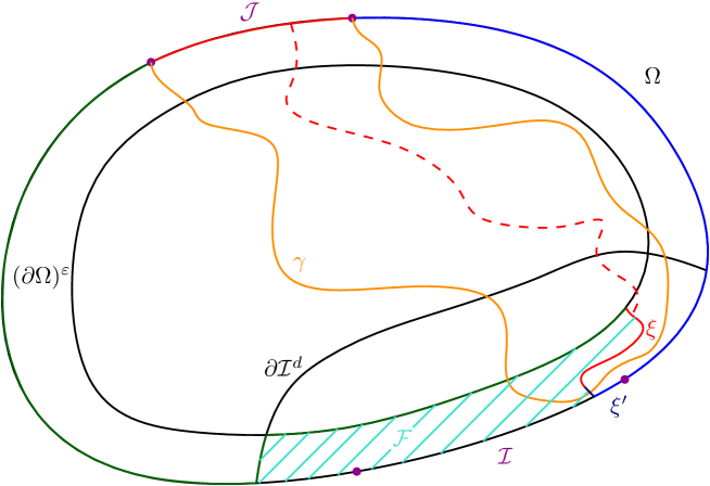
Figure 6.1. In the domain $\Omega$, with boundary arcs $\mathcal{I}$ and $\mathcal{J}$ materialized by their extremities (purple points), we consider the Ising model with mixed boundary conditions $\mathbb{P}^{+/-}$, conditioned on $\xi$ to exist, and on $\mathcal{F}$, the data of the state of all spins in the dashed turquoise region. We obtain an Ising model in a quad whose boundary consists of $\mathcal{J}$ (carrying $-$ spins, in red) ; the green path, carrying mixed spins ; the curve $\xi$ carrying $-$ spins, in red ; and a blue curve (in two shades), carrying mixed spins. RSW estimates ensure the existence with uniformly positive probability of a strong path of $-$ spins (dashed red) in this quad. This path forces the Ising interface $\gamma$ generated by the mixed boundary conditions on $\Omega$ to get close to $\partial\Omega$ at the base of $\xi$.

Let us fix sequences $\eta_{k}\to 0$ as $k\to\infty$ and $\delta_{n,k}\to 0$ as $n\to\infty$ such that for all $n,k$ we have

$$\mathbb{P}^{+/-}\left(E_{\delta_{n,k}}\left(\eta_{k},\varepsilon,\mathcal{I}\right)\right)\geq\frac{\alpha^{\prime}}{2}>0.$$

Let us consider the first crossing $\xi$ of $-$ spins in $\mathcal{I}^{d}$ from $\mathcal{I}^{\eta_{k}}$ to $\Omega\setminus(\partial\Omega)^{\varepsilon}$ in counterclockwise order. We arbitrarily extend $\xi$ to $\partial\Omega$ by adding to it a path $\xi^{\prime}$ staying in $\mathcal{I}^{\eta_{k}}$

We condition on the data $\mathcal{F}$ of all the Ising spins included in $\mathcal{I}^{d}$ to the left of $\xi\cup\xi^{\prime}$. Conditionally on $\xi$ to exist, and on the data $\mathcal{F}$, the law of the remaining spins is given by an Ising model in a quad, where two of the opposing boundary subintervals ($\xi$ and $\mathcal{J}$) carry $-$ spins (see Figure 6.1). Moreover, the extremal length of this quad is bounded, uniformly in $\xi$, $\delta$.

By RSW-type estimates [CDH16, Corollary 1.7], we obtain that with (uniformly) positive probability, $\xi$ is connected by a path of $-$ spins to the $-$ spins of $\mathcal{J}$. This implies that the Ising interface generated by the $\pm$ boundary condition hits $\mathcal{I}^{\eta_{k}}$. Passing to the limit $n\to\infty$ and then $k\to\infty$ implies that the scaling limit of the interface generated by the boundary conditions hits $\mathcal{I}$ with positive probability, which is a contradiction: the scaling limit is $\mathrm{SLE}_{3}$ [CDHKS14, Theorem 1], which never hits the boundary of the domain it lives in [Law05, Proposition 6.8]. ∎

Proof of Lemma 15.

Lemma 16 shows that the scaling limits of Ising loops almost surely either do not touch the boundary or are included in it. However, this second possibility almost surely does not happen, as Ising loops are included in cut-out domains of the scaling limits of the FK loops, themselves described by a branching $\mathrm{SLE}_{16/3}\left(-2/3\right)$. On the event that an Ising loop is included in the boundary, the same would have to be true of a piece of $\mathrm{SLE}_{16/3}\left(-2/3\right)$, which cannot happen.

The interested reader can find an inspiration for an argument that does not use the FK coupling but RSW-type considerations instead in [BDH16, Lemma 18] ∎

Lemma 17.

The scaling limit of the outermost Ising loops are almost surely simple and do not touch each other.

Proof.

As explained in the proof of Lemma 13, we can discover the collection of outermost Ising loops $\mathcal{L}_{1}$ through the iteration of an exploration process of FK loops and Ising arcs. At the $n$-th, step, we discover a sub-collection $\mathcal{L}_{n}$

Two Ising loops with different discovery times $m<n$ do not touch each other in the scaling limit. Indeed, the loops in $\cup_{n>m}\mathcal{L}_{n}$ (i.e., the loops that are discovered at times strictly larger than $m$) are outermost loops within one of the cut-out domains of the collection $\mathcal{R}_{m}$. By Lemma 15, the loops in $\cup_{n>m}\mathcal{L}_{n}$ stay strictly inside the domains of $\mathcal{R}_{n}$ (with the notation of the proof of Lemma 13) and hence cannot intersect the loops in $\mathcal{L}_{m}$

We now show that the loops of a sub-collection $\mathcal{L}_{m}$ are almost surely simple and do not touch each other. Recall that these Ising loops are recovered by gluing arcs of a FAE staying in a cut-out domain of some FK loops (in the collection $\mathcal{R}_{m}$). By Proposition 24, the boundaries of cut-out domains in $\mathcal{R}_{m}$ are simple disjoint curves. Moreover, the Ising loops that stay within a single cut-out domain are simple and disjoint: indeed, these loops are constructed by gluing arcs of the FAE, which is a family of simple disjoint arcs. ∎

Lemma 18.

In the scaling limit, the outermost Ising loops satisfy the domain Markov property.

Proof.

This directly follows from the discrete Markov property, together with the convergence of outermost Ising loops for any discrete approximation of the continuous domain (Lemma 13). ∎

Finally, we will need to identify the value of the parameter $\kappa=3$.

Lemma 19.

Consider the scaling limit of the outermost Ising loops. Almost surely, there is a subarc of a loop that has Hausdorff dimension 11/8.

Proof.

As explained in the proof of Lemma 13, the Ising loops can be constructed by gluing arcs of the FAE, which are pieces of an $\mathrm{SLE}_{3}\left(-\frac{3}{2},-\frac{3}{2}\right)$ exploration tree. As a result, Ising loops have subarcs that have Hausdorff dimension 11/8 (see [Bef08]). ∎

6.2. Proof of Theorem 6

Proof.

The outermost Ising loops have a conformally invariant scaling limit (Lemma 13). By Lemmas 15 and 17, the loops of the scaling limit are simple and do not touch each other or the boundary. By Lemma 18, these loops satisfy the Markovian restriction property. Hence, by the Sheffield-Werner Markovian characterization property, the scaling limit of the outermost Ising loops is a $\mathrm{CLE}_{\kappa}$ for some $\frac{8}{3}<\kappa\leq 4$. By Lemma 19 and the construction of $\mathrm{CLE}_{\kappa}$ in terms of $\mathrm{SLE}_{\kappa}$-like loops [She09], we deduce that $\kappa$ must be equal to $3$.

We now establish the convergence of the Ising loops of level $2$. These loops lay inside of the outermost Ising loops, i.e. are loops of an Ising configuration with $-$ boundary conditions. The set of leftmost loops in a domain with $-$ boundary conditions has the same law as the set of rightmost loops in a domain with $+$ boundary conditions. By the second part of Lemma 14, the scaling limit of level 2 loops is hence given by independent $\mathrm{CLE}_{3}$ in each of the level 1 loops. Further iterating this argument, we identify the set of loops of level $n$ as independent $\mathrm{CLE}_{3}$ inside the loops of level $n-1$.

Moreover, a corollary of Lemma 12 is that the supremum of the diameters of the Ising loops of level $n$ goes to $0$ in probability as $n\to\infty$, uniformly in the mesh size $\delta$. Hence the convergence of the set of all Ising loops to nested $\mathrm{CLE}_{3}$ follows from the convergence of the Ising loops of level $n$, for each fixed $n$. ∎

Appendix A FK interfaces have a conformally invariant scaling limit

In this section, we prove Proposition 11: we show that for any Jordan domain $\Omega$, the set of all level one (outermost) FK loops in $\Omega$ converges towards a conformally invariant limit (see also [KeSm15] for an alternative approach). We prove the convergence of a single FK exploration path (Lemma 20) without smoothness assumptions on $\partial\Omega$.

We rely on [KeSm12] to get tightness of the exploration path, and we rely on the convergence result [CDHKS14, Theorem 2] together with an argument similar to the one used in [BDH16] to identify the scaling limit. Once we know the convergence of a single exploration, we can deduce the convergence of all outermost FK loops by iteratively using the convergence of FK exploration interfaces (Proposition 22).

Let us also point out that [KeSm16] have recently given an alternative proof of the results stated here, with a more in-depth description of the relevant loops.

A.1. Convergence of FK interfaces

Consider a discrete domain $\Omega_{\delta}$, with dual $\Omega_{\delta}^{*}$ and bi-medial $\Omega_{\delta}^{b}$. Consider an FK model configuration $\omega$ on $\Omega_{\delta}$ with wired boundary conditions and its dual configuration $\omega^{*}$. Given boundary bi-medial points $a$ and $b$, we define the FK exploration $\gamma_{\delta}$ of $\omega$ from $a$ to $b$ as follows:

• $\gamma_{\delta}$ is a simple path on the bi-medial graph of $\Omega_{\delta}$ from $a$ to $b$

• when $\gamma_{\delta}$ is not on the boundary $\partial\Omega_{\delta}^{b}$, $\gamma_{\delta}$ follows the primal boundary cluster of $\omega$ on its left and a dual cluster of $\omega^{*}$ on its right

• when $\gamma_{\delta}$ is on $\partial\Omega_{\delta}^{b}$, $\gamma_{\delta}$ keeps a dual cluster on its right whenever possible (i.e. with the constraint that $\gamma_{\delta}$ is simple and goes from $a$ to $b$).

The following result gives us that the interface $\gamma_{\delta}$ converges to the ${\rm SLE}_{\kappa}(-\rho)$ process with $\kappa=16/3$ and $\rho=\kappa-6$ (see e.g. [ScWi05, She09]).

Lemma 20.

Let $\Omega_{\delta}$ be a discrete approximation of a Jordan domain $\Omega$ and let $a_{\delta},b_{\delta}\in\partial\Omega_{\delta}^{b}$ with $a_{\delta},b_{\delta}\to a,b\in\partial\Omega$. Let $\gamma_{\delta}$ be the FK exploration from $a_{\delta}$ to $b_{\delta}$. Then $\gamma_{\delta}$ converges in law to an ${\rm SLE}_{16/3}(-2/3)$ curve, with respect to the supremum norm up to reparametrization.

Proof.

For any discrete time step $n\geq 0$, let us denote by $\Omega_{n,\delta}$ the connected component of $\Omega_{\delta}\setminus\gamma_{\delta}\left[0,n\right]$ containing $b$. Let us denote by $O_{n,\delta}$ the clockwise-most point of $\partial\Omega_{n,\delta}\cap\partial\Omega_{\delta}$ (i.e. the rightmost intersection of $\gamma_{\delta}\left[0,n\right]$ with $\partial\Omega_{\delta}$). Conditionally on $\gamma_{\delta}\left[0,n\right]$, the configuration $\omega$ in $\Omega_{n,\delta}$ is an FK configuration with boundary conditions that are free on the right of $\gamma_{\delta}$ (i.e. on the counterclockwise arc $\left[\gamma_{\delta}\left(n\right),O_{n,\delta}\right]$) and wired elsewhere.

Analogously to the reasoning made in [BDH16], we can use the crossing estimates of [CDH16] on the domains $\left(\Omega_{n,\delta}\right)$ to apply the technology of [KeSm12, Theorems 3.4 and 3.12] which allows us to obtain that the law of the exploration $\gamma_{\delta}$ is tight.

Let us now consider an almost sure scaling limit $\gamma$ of $\gamma_{\delta_{k}}$ for $\delta_{k}\to 0$ (which is possible via the Skorokhod embedding theorem). Consider a conformal mapping $\Omega\to\mathbb{H}$ with $(a,b)\mapsto(0,\infty)$ and denote by $\lambda$ the image of $\gamma$. Encode $\lambda$ by a Loewner chain, i.e. consider the family of conformal mappings $g_{t}:H_{t}\to\mathbb{H}$, where $H_{t}$ is the unbounded connected component of $\mathbb{H}\setminus\lambda\left[0,t\right]$ and we normalize $t$ and $g_{t}$ such that, for any time $t$, $g_{t}\left(z\right)=z+2t/z+o\left(1/z\right)$ as $z\to\infty$. Set $U_{t}:=g_{t}\left(\lambda\left(t\right)\right)$ and $O_{t}:=\sup\left(\lambda\left[0,t\right]\cap\mathbb{R}\right)$. As usual, we have the Loewner equation $\partial_{t}g_{t}\left(z\right)=2/\left(g_{t}\left(z\right)-U_{t}\right)$ and as a result $U_{t}$ characterizes $\lambda$ and hence $\gamma$.

Let us now characterize the law of $U_{t}$. Set

$$X_{t}:=\frac{O_{t}-U_{t}}{\sqrt{16/3}}.$$

The following two properties allow one to prove that $X_{t}$ is a Bessel process of dimension $d=3/2$ (as in [BDH16]):

• The process $X_{t}$ is instantaneously reflecting off $0$, i.e the set of times $\left\{t:X_{t}=0\right\}$ has zero Lebesgue measure: this is a deterministic property for Loewner chains (see e.g. [MS16, Lemma 2.5]). This imply that $X_{t}$ can be deterministically recovered from the ordered set of its excursions away from $0$.

• When $X_{t}$ is away from $0$, the tip of the curve $\gamma\left(t\right)$ is away from the boundary arc $\left[a,b\right]$. This corresponds in the discrete to a time $t$ when the curve $\gamma_{\delta_{k}}\left(t\right)$ is away from the boundary arc $\left[a_{\delta_{k}},b_{\delta_{k}}\right]$, and hence the domain yet to be explored $\Omega_{t,\delta_{k}}$ has ‘macroscopic Dobrushin conditions’ in the sense that both the wired and free boundary arcs are macroscopic. By [CDHKS14, Theorem 2], the curve $\lambda$ behaves as chordal $\mathrm{SLE}\left(16/3\right)$ headed towards $O_{t}$ until the first hitting time of $[O_{t},+\infty)$, which is the same, by SLE coordinate change [ScWi05], as an SLE${}_{16/3}(-2/3)$ with force point at $O_{t}$ until the first hitting time of $[O_{t},+\infty)$. Hence, the law of the ordered set of excursions of $X_{t}$ away from $0$ is that of the ordered set of excursions of a Bessel process of dimension $d=3/2$ away from $0$.

Let us now identify the process $O_{t}$. By integrating the Loewner equation, we find that

$$O_{t}=\int_{0}^{t}\frac{2}{\sqrt{16/3}\;X_{s}}ds+A_{t},$$

where $A_{t}$ is constant when $X_{t}$ is away from $0$. The following argument yields that $A_{t}$ is constant equal to zero:

• The process $X_{t}$ is $\left(\frac{1}{2}\right)^{-}$-Hölder continuous, as a Bessel process.

• Since $d=3/2>1$, we have that

  $$I_{t}=\int_{0}^{t}\frac{2}{\sqrt{16/3}\;X_{s}}ds$$

  is almost surely finite, and moreover $I_{t}$ is $\left(\frac{1}{2}\right)^{-}$-Hölder continuous (as can be seen from the fact that $X_{t}-I_{t}$ is a standard Brownian motion).

• By the tightness result of [KeSm12] (see [KeSm12, Theorems 3.4 and 3.12]), the driving function $U_{t}$ must be a.s. $\left(\frac{1}{2}\right)^{-}$-Hölder continuous.

• As $A_{t}=\sqrt{16/3}\;X_{t}+U_{t}-I_{t}$, we see that $A_{t}$ must be $\left(\frac{1}{2}\right)^{-}$-Hölder continuous.

• Since $A_{t}$ can only vary on the set $\left\{t:X_{t}=0\right\}$, whose dimension is $\frac{2-d}{2}=\frac{1}{4}<\frac{1}{2}$, $A_{t}$ must be constant (as in [BDH16, Lemma 9] or [KeSm15, Section 5.4]).

This characterizes the law of the pair $\left(X_{t},O_{t}\right)$, and hence the law of the driving function $U_{t}$: the curve $\lambda$ is an SLE${}_{16/3}(-2/3)$ process, with force point starting at $0^{+}$. ∎

A.2. Special points of FK interfaces

The goal of Section A.3 will be to describe a conformally invariant exploration procedure which for any $\varepsilon>0$, with high probability as $\delta\to 0$, gives $\varepsilon$-approximations of all the level one FK loops of diameter larger than $\varepsilon$.

In order to do so, we need to control the formation of continuous cut-out domains, i.e. we need to understand what happens on the lattice level when the scaling limit of the interface has a double point or touches the boundary. We only need to control what happens on the right side of the curve $\gamma_{\delta}$, as the arguments needed to control the left side are similar. Let us now introduce the following subsets of $\gamma_{\delta}$ (resp. $\gamma$):

• The set $\mathcal{P}_{B}$ of right boundary points is the set of points $x$ where the interface $\gamma_{\delta}$ comes as close as possible to the counter-clockwise boundary arc from $a$ to $b$, i.e. a bi-medial mesh size $\delta/2$ away (resp. $\gamma$ touches the boundary arc $\left[a,b\right]$ in the continuous).

• The set $\mathcal{P}_{D}$ of clockwise double points is the set of points $x$ where $\gamma_{\delta}$ comes within distance $\delta/2$ of a point $x^{\prime}$ of its past (resp. $x$ is a double point of $\gamma$), and such that the interface winds clockwise from $x^{\prime}$ to $x$.

We call points of $\mathcal{P}_{B}\cup\mathcal{P}_{D}$ special points. For a special point $x\in\mathcal{P}_{B}\cup\mathcal{P}_{D}$ of $\gamma_{\delta}$ (resp. $\gamma$), we define the subpath $K\left(x\right)$ of $\gamma_{\delta}$ (resp. of $\gamma$) as follows:

• If $x\in\mathcal{P}_{B}$, $K(x)$ is the whole part of the curve running from the origin $a$ to $x$ (excluding $a$ and $x$).

• If $x\in\mathcal{P}_{D}$, $K(x)$ is the loop the curve forms at $x$ (excluding $x$), i.e. the part of the curve $\gamma_{\delta}$ (resp. $\gamma$) running from $x^{\prime}$ to $x$, where $x^{\prime}$ is as above. Note that this is well-defined in the continuum, as the FK interface does not have triple points: this would indeed imply a six-arm event primal-dual-primal-dual-primal-dual that is ruled out by [CDH16, Remark 1.6].

Note that for any special points $x,y\in\mathcal{P}_{B}\cup\mathcal{P}_{D}$, if $K(x)\cap K(y)\neq\emptyset$, then either $K(x)\subseteq K(y)$ or $K(y)\subseteq K(x)$.

Given a finite family of points $\mathcal{P}\subset\mathcal{P}_{B}\cup\mathcal{P}_{D}$ containing the endpoint $b$, we define the partition $(P(x))_{x\in\mathcal{P}}$ of $\gamma_{\delta}\setminus\{a,b\}$ (resp. $\gamma\setminus\{a,b\}$) by:

$$P(x):=K(x)\setminus\bigcup_{y\in\mathcal{P}:K(y)\subset K(x)}K(y).$$

Note that $P(x)$ is always a non-self-crossing loop (minus a point) or a non-self-crossing path joining two boundary points. For $x\in\mathcal{P}$, we say that $P\left(x\right)$ is an $\varepsilon$-approximation of a cut-out domain if (at least) one of the following holds:

• The set $P(x)$ is of diameter less than $2\varepsilon$.

• We can write the set $P(x)$ as

  $$P(x)=\left((\partial D\cap\Omega)\setminus{x}\right)\cup\bigcup_{{\gamma^{\prime}}\in\mathcal{C}}{\gamma^{\prime}},$$

  where $D$ is a cut-out domain laying on the right side of $\gamma_{\delta}$ (resp. $\gamma$), and $\mathcal{C}$ is a collection of paths of diameter less than $\varepsilon$, with one endpoint on $\partial D\setminus{x}$

We say that a finite family of special points $\mathcal{P}\subset\mathcal{P}_{B}\cup\mathcal{P}_{D}$ is an $\varepsilon$-pinching family if for each point $x\in\mathcal{P}$, $P\left(x\right)$ is an $\varepsilon$-approximation of a cut-out domain.

The main statement of this subsection is that double points of the scaling limit correspond to double points of the discrete interface (and similarly for the boundary points). More precisely, we have the following:

Proposition 21.

For all $\varepsilon,\varepsilon^{\prime}>0$, there is a mesh size $\delta_{0}>0$, such that for all $\delta<\delta_{0}$, the following holds:

We can couple $\gamma_{\delta}$ and $\gamma$, find an $\varepsilon$-pinching family $\mathcal{P}^{\varepsilon}$ of $\gamma$ and parametrize $\gamma_{\delta}:\left[0,1\right]\to\Omega_{\delta}$ and $\gamma:\left[0,1\right]\to\bar{\Omega}$ so that, with probability at least $1-\varepsilon^{\prime}$:

1. For any special point $x\in\mathcal{P}^{\varepsilon}$, there is a special point $x_{\delta}$ of $\gamma_{\delta}$ such that the subpaths $K(x_{\delta})$ and $K(x)$ are parametrized by the same time intervals.

2. The parametrized curves $\gamma_{\delta}$ and $\gamma$ are $\varepsilon$-close to each other in the topology of supremum norm.

Proof.

By contradiction, assume there is $\varepsilon,\varepsilon^{\prime}$ and a sequence of mesh size $\delta_{n}\to 0$ such that we cannot do the required construction for any of the values $\delta_{n}$. By Skorokhod embedding theorem, and the convergence in law of $\gamma_{\delta}\to\gamma$, we can construct a coupling of $\gamma_{\delta_{n}}$ and $\gamma$ such that $\gamma_{\delta_{n}}\to\gamma$ almost surely. Let us construct discrete $\varepsilon/2$-pinching families $\mathcal{P}_{\delta_{n}}^{\varepsilon}$, and show that we can extract a subsequence $\left(\delta_{k}\right)\subset\left(\delta_{n}\right)$ such that $(\gamma_{\delta_{k}},\mathcal{P}_{\delta_{k}}^{\varepsilon})$ converges almost surely to $(\gamma,\mathcal{P}^{\varepsilon})$, where $\mathcal{P}^{\varepsilon}$ is a finite $\varepsilon$-pinching family (and convergence of pinching points is in the sense of (1) in the statement of the theorem). This will provide a contradiction, and hence imply the claim.

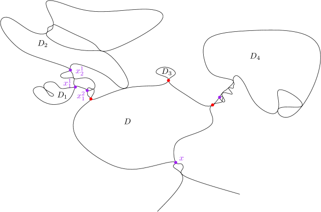
Figure A.1. A cut-out domain $D$ of diameter larger than $\varepsilon$ (the scale is given in orange). It is bounded by pieces of $\gamma$, and clockwise double points, shown in red. Some of these double points disconnect pieces of diameter less than $2\varepsilon$ (the domain $D_{3}$ is one of these). The other (macroscopic) double points are controlled on the discrete level by purple pinching points (disconnecting $D_{1}$, $D_{2}$ and $D_{4}$). Note that in this picture the point $x_{2}^{2}$ is equal to $x_{1}^{2}$.

Let us now consider the finite family $\left(w_{k}\left(\delta\right)=\gamma_{\delta}\left(s_{k}\right)\right)_{k=0,\ldots,n}$ of points on $\gamma_{\delta}$ in chronological order, with

• $w_{0}\left(\delta\right)=a$ and $w_{n}\left(\delta\right)=b$

• for any $0<i<n$, $s_{i}$ is the first time after $s_{i-1}$ when $\gamma_{\delta}$ exits the ball of radius $\varepsilon/4$ around $w_{i-1}\left(\delta\right)$,

• $\mathrm{diam}\left(\gamma_{\delta}\left[s_{n-1},s_{n}\right]\right)\leq\varepsilon/4$.

We then define a finite $\varepsilon/2$-pinching family $\mathcal{P}_{\delta}^{\varepsilon}$ of points $x_{i}^{j}\left(\delta\right)=\gamma_{\delta}\left(t_{i}^{j}\left(\delta\right)\right)$ (that may not be distinct) in the following way:

• Let $x_{i}^{0}\left(\delta\right)$ be the first point of $\mathcal{P}_{B}\cup\mathcal{P}_{D}$ coming after $w_{i}\left(\delta\right)$ such that $K\left(x_{i}^{0}\left(\delta\right)\right)$ contains $w_{i}\left(\delta\right)$ and is of diameter at least $\varepsilon/2$.

• For $j\geq 0$, we define $x_{i}^{j+1}\left(\delta\right)$ as the first point after $x_{i}^{j}\left(\delta\right)$ such that $K(x_{i}^{j}\left(\delta\right))\subset K(x_{i}^{j+1}\left(\delta\right))$ and such that the diameter of $K(x_{i}^{j+1}\left(\delta\right))\setminus K(x_{i}^{j}\left(\delta\right))$ is at least $\varepsilon/2$.

Let us explain why $\mathcal{P}_{\delta}^{\varepsilon}$ is an $\varepsilon/2$-pinching family (see Figure A.1).

• Suppose $y$ is a special point of $\gamma_{\delta}$ such that ${\rm diam}K(y)\geq\varepsilon/2$. Then $K(y)$ contains at least one point $w_{i}(\delta)$. Let $j$ be the highest index such that $x_{i}^{j}(\delta)\in K(y)$. Then we have that either $y=x_{i}^{j}(\delta)$, or that $K(y)\setminus K(x_{i}^{j}(\delta))$ is of diameter less than $\varepsilon/2$. In particular, for any special point $y$, we have that either $y\in\mathcal{P}_{\delta}^{\varepsilon}$ or that the diameter of

  $$K(y)\setminus\bigcup_{x_{i}^{j}\left(\delta\right)\in\mathcal{P}_{\delta}^{\varepsilon}:K(x_{i}^{j}\left(\delta\right))\subset K(y)}K(x_{i}^{j}\left(\delta\right))$$

  is less than $\varepsilon/2$.

• Every special point $x$ of $\gamma_{\delta}$ is the closing point of a (possibly degenerate, i.e. of diameter $\delta/2$) cut-out domain $D_{x}$. Moreover, the set

  $$K(x)\setminus\bigcup_{y\in\mathcal{P}_{B}\cup\mathcal{P}_{D}:K(y)\subset K(x)}K(y)$$

  corresponds to the parts of $\gamma_{\delta}$ that trace the boundary of the cut-out domain $D_{x}$.

• By the two previous items, for any $x_{i}^{j}\left(\delta\right)\in\mathcal{P}_{\delta}^{\varepsilon}$, we have that

  $$P(x_{i}^{j}\left(\delta\right))=D_{x_{i}^{j}(\delta)}\bigcup\left(\bigcup_{y\in\partial D_{x_{i}^{j}(\delta)}\cap(\mathcal{P}_{B}\cup\mathcal{P}_{D}\setminus\mathcal{P}_{\delta}^{\varepsilon})}\left(K(y)\setminus\bigcup_{x_{k}^{l}(\delta)\in\mathcal{P}_{\delta}^{\varepsilon}\cap K(y)}K(x_{k}^{l}(\delta))\right)\right)$$

  can be obtained by attaching to $D_{x_{i}^{j}\left(\delta\right)}$ paths of diameter less than $\varepsilon/2$ and hence is an $\varepsilon/2$-approximation of a cut-out domain.

Note that the number of points in $\mathcal{P}_{\delta}^{\varepsilon}$ is tight, as the almost sure limit $\gamma$ of the $\gamma_{\delta_{n}}$ is a continuous curve. By compactness, we can assume that the family $\mathcal{P}_{\delta}^{\varepsilon}$ converges to a finite family $\mathcal{P}^{\varepsilon}$ of points $x_{i}^{j}=\gamma(t_{i}^{j})$ on the curve $\gamma$ (at least by taking a subsequence $\gamma_{\delta_{k}}$) in the following sense: we can parametrize $\gamma_{\delta_{k}}$ and $\gamma$ such that for these parametrizations $\|\gamma_{\delta_{k}}-\gamma\|_{\infty}\to 0$ almost surely, such that the limit $t_{i}^{j}:=\lim t_{i}^{j}\left(\delta_{k}\right)$ exists for all $i,j$, and such that for any $x\in\mathcal{P}^{\varepsilon}$, there exists a point $x_{\delta}\in\mathcal{P}_{\delta}^{\varepsilon}$ such that the subpaths $K(x_{\delta})$ and $K(x)$ are parametrized by the same time intervals. The claim of the proposition hence reduces to proving that the family $\mathcal{P}^{\varepsilon}$ is an $\varepsilon$-pinching family for $\gamma$, namely that for any $x_{i}^{j}=\gamma\left(t_{i}^{j}\right)\in\mathcal{P}^{\varepsilon}$, the set $P\left(x_{i}^{j}\right)$ is an $\varepsilon$-approximation of a cut-out domain. In the following, we will assume that $x_{i}^{j}\in\mathcal{P}_{D}$. The case $x_{i}^{j}\in\mathcal{P}_{B}$ follows from similar arguments and is simpler.

To prove this, let us first introduce approximations $x_{i}^{j}\left(\delta,\eta\right)=\gamma_{\delta}\left(t_{i}^{j}\left(\delta,\eta\right)\right)$ of the $\varepsilon$-pinching points $x_{i}^{j}(\delta)$ for $\eta>0$. The point $x_{i}^{j}\left(\delta,\eta\right)$ is defined to be the first point after $x_{i}^{j-1}\left(\delta\right)$ (or after $w_{i}\left(\delta\right)$ if $j=0$) to be $\eta$-close to being a macroscopic pinching point, i.e. such that if $\gamma_{\delta}$ were to continue along a (hypothetical) path $\tilde{\gamma}$ of length at most $\eta$, the pinching point $x_{i}^{j}\left(\delta\right)$ would be located at the end of $\tilde{\gamma}$.

Consider the family of points $y_{i}^{j}$ located at times $u_{i}^{j}:=\lim_{\eta_{m}\to 0}\lim_{\delta_{k}\to 0}t_{i}^{j}\left(\delta_{k},\eta_{m}\right)$ (where the double limit $\delta_{k}\ll\eta_{m}\ll 1$ is taken through a diagonal extraction if necessary). It remains to show that with high probability, each point $y_{i}^{j}=\gamma\left(u_{i}^{j}\right)$ appears chronologically right before the point $x_{i}^{j}$, in the sense that $\mathrm{diam}\left(K(x_{i}^{j})\setminus K(y_{i}^{j})\right)\leq\varepsilon/2$. This will readily imply that $P\left(x_{i}^{j}\right)$ is an $\varepsilon$-approximation of a cut-out domain, thus concluding the proof of the proposition.

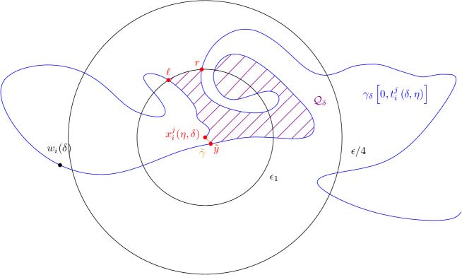
Figure A.2. The quad $\mathcal{Q}_{\delta}$ in striped purple. Primal and dual FK crossings in this quad will force the appearance of the pinching point $x_{i}^{j}(\delta)$ before $\gamma_{\delta}$ touches the arc $[r,\ell]$.

Let us now fix a point $y_{i}^{j}$. We want to find a quad (i.e. a topological rectangle) $\mathcal{Q}_{\delta}$ that contains (with high probability) FK crossings ensuring that the set $K(x_{i}^{j})\setminus K(y_{i}^{j})$ is small. For $\alpha>0$, let us define the ball $B_{\alpha}:=\left\{z\in\Omega_{\delta}:\left|z-x_{i}^{j}\left(\delta,\eta\right)\right|<\alpha\right\}$ of radius $\alpha$ around $x_{i}^{j}\left(\delta,\eta\right)$, and let $T_{\alpha}$ be the set of times when $\gamma_{\delta}$ visits this ball:

$$T_{\alpha}\left(\delta,\eta\right):=\left\{t\in\left[0,t_{i}^{j}\left(\delta,\eta\right)\right]:\gamma_{\delta}(t)\in B_{\alpha}\right\}.$$

The curve $\gamma$ does not have triple points, as this would produce a six-arm event prevented by [CDH16, Remark 1.6]. In particular $y_{i}^{j}$ is not a triple point for $\gamma$. As a result, we can pick $\varepsilon_{1}>0$ small enough such that for all $\delta\ll\eta\ll\varepsilon_{1}$, we have that $T_{\varepsilon_{1}}\left(\delta,\eta\right)$ is included in two connected components of $T_{\varepsilon/4}$ with high probability: one of the connected components containing $t_{i}^{j}\left(\delta,\eta\right)$, and the other one containing the end $\tilde{y}$ of the (hypothetical) curve $\tilde{\gamma}$ considered above (see Figure A.2).

Let us now define the quad $\mathcal{Q}_{\delta}$, with boundary marked points $r,\ell,x_{i}^{j}\left(\delta,\eta\right)$ and $\tilde{y}$ (in counterclockwise order):

• the segment $\left[r,\ell\right]$ is the connected component of $\partial B_{\varepsilon_{1}}\setminus\gamma_{\delta}\left[0,t_{i}^{j}\left(\delta,\eta\right)\right]\cap\partial B_{\varepsilon_{1}}$ that disconnects $x_{i}^{j}\left(\delta,\eta\right)$ from the endpoint $b$ of $\gamma_{\delta}$ in the domain $\Omega_{\delta}\setminus\gamma_{\delta}\left[0,t_{i}^{j}\left(\delta,\eta\right)\right]$;

• the segments $\left[\ell,x_{i}^{j}\left(\delta,\eta\right)\right]$ and $\left[\tilde{y},r\right]$ follow $\gamma_{\delta}$;

• the segment $\left[x_{i}^{j}\left(\delta,\eta\right),\tilde{y}\right]$ is simply $\tilde{\gamma}$.

By choosing $\eta$ small enough (and $\delta\ll\eta$), we can make the extremal distance (see [CDH16] for a definition) between the arcs $\left[\ell,x_{i}^{j}\left(\delta,\eta\right)\right]$ and $\left[\tilde{y},r\right]$ in $\mathcal{Q}_{\delta}$ arbitrarily small. By the RSW estimate of [CDH16], we can ensure that with arbitrarily high probability (for any $\delta$ small enough), there is a dual FK crossing separating $\left[x_{i}^{j}\left(\delta,\eta\right),\tilde{y}\right]$ from $\left[r,\ell\right]$ and furthermore a primal FK crossing separating the dual crossing from $\left[r,\ell\right]$. As a result, there is a point $z_{\ell}\in\left[\ell,x_{i}^{j}\left(\delta,\eta\right)\right]$ and a point $z_{r}\in\left[\tilde{y},r\right]$ between which $\gamma_{\delta}$ has to travel while staying within $\mathcal{Q}_{\delta}$. In particular, $z_{r}$ is a special point of $\gamma_{\delta}$ such that $K(x_{i}^{j-1}(\delta))\subset K(z_{r})$ (resp. such that $w_{i}(\delta)\in K(z_{r})$ if $j=0$) and such that $K(z_{r})\setminus K(x_{i}^{j-1}(\delta))$ encloses $\tilde{\gamma}$ and hence is of diameter larger than $\varepsilon/2$. This ensures that the point $x_{i}^{j}(\delta)$ is found before the point $z_{r}$, in particular before $\gamma_{\delta}$ crosses the arc $[r,\ell]$. As $y_{i}^{j}$ is not a triple point for the curve $\gamma$, and as the quad $\mathcal{Q}_{\delta}$ is of diameter less than $\varepsilon/2$, we see that with high probability, $\gamma\left[t_{i}^{j}(\eta),t_{i}^{j}\right]$ is of diameter less than $\varepsilon/2$ and hence with high probability the set $K(x_{i}^{j})\setminus K(y_{i}^{j})$ is of diameter less than $\varepsilon/2$.

By taking the successive limits $\delta\ll\eta\ll\varepsilon_{1}\ll\varepsilon$, we obtain that all $P\left(x_{i}^{j}\right)$ are $\varepsilon$-approximations of a cut-out domain, and hence that $\mathcal{P}^{\varepsilon}$ is an $\varepsilon$-pinching family, thus proving the proposition. ∎

A.3. Convergence of FK loops

In this subsection, we identify the scaling limit of the outermost FK loops by a recursive exploration procedure (see Figure A.3), analogous to the exploration procedure introduced in [CaNe07b].

Proposition 22.

The set of all level 1 FK loops in the discrete approximation $\Omega_{\delta}$ of a Jordan domain $\Omega$ with wired boundary conditions converges to a conformally invariant scaling limit.

Proof.

Let us fix $\varepsilon>0$ and define an exploration procedure (see [CaNe07b] for a similar construction) that will discover all the level one FK loops of diameter at least $\varepsilon$. Note that, in order to see that the $d_{\mathcal{X}}$ distance is smaller than $\varepsilon$, only the loops of diameter at least $\varepsilon$ matter.

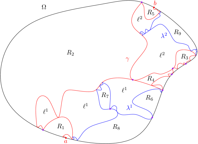
Figure A.3. In red, the first exploration path. It cuts out $k=2$ domains with mixed boundary conditions and large diameter, as well as five domains $R_{1},\ldots,R_{5}$ with wired boundary conditions and large diameter. The mixed boundary conditions domain are further cut by two blue explorations $\lambda^{1}$ and $\lambda^{2}$. These cut out four more large domains with wired boundary conditions, and allows us to recover two FK loops: the three domains $R_{6},R_{7},R_{8}$ and the loop $\ell_{1}$ for $\lambda^{1}$; and the domain $R_{9}$ and the loop $\ell_{2}$ for $\lambda^{2}$. The purple dots are special discrete points with very high probability (as they are $\varepsilon$-pinching points).

Let us choose boundary bi-medial points $a_{\delta},b_{\delta}\in\partial\Omega_{\delta}^{b}$ converging to points $a,b\in\partial\Omega$, and consider the exploration path $\gamma_{\delta}$ from $a_{\delta}$ to $b_{\delta}$, as in Lemma 20. Let us condition on $\gamma_{\delta}$ and consider the connected components of $\Omega_{\delta}\setminus\gamma_{\delta}$:

• The connected components on the left side of $\gamma_{\delta}$ have wired boundary conditions.

• The components on the right side of $\gamma_{\delta}$ that touch the boundary of $\Omega_{\delta}$ have mixed boundary conditions.

• All other components stay on the right side of $\gamma_{\delta}$ and have free boundary conditions.

Let us consider the macroscopic domains cut-out by $\gamma_{\delta}$, i.e., the connected components of $\Omega_{\delta}\setminus\gamma_{\delta}$ of diameter at least $\varepsilon$. As $\delta\to 0$, the interface $\gamma_{\delta}$ converges to a continuous curve, namely an $\mathrm{SLE}_{16/3}\left(-2/3\right)$, (Lemma 20) and as all double points of this limit correspond to discrete double points of $\gamma_{\delta}$ (Proposition 21), we see that, uniformly in the mesh size $\delta$, with high probability there are at most $N$ macroscopic domains cut-out by $\gamma_{\delta}$, for $N$ large enough.

In each of these macroscopic domains $D_{\delta}^{j}$ (for $j=1,\ldots,k\leq N$) that have mixed boundary conditions, we consider the FK interface $\lambda_{\delta}^{j}$ that separates the wired and the free boundary arcs. We obtain $k$ FK loops $\ell_{\delta}^{j}$ by concatenating each interface $\lambda_{\delta}^{j}$ with the arc of $\gamma_{\delta}$ joining its endpoints. Moreover, each of the $\lambda_{\delta}^{j}$ cuts the mixed domain into a collection of domains with free boundary conditions (these are the cut-out domains of $\ell_{\delta}^{j}$) and domains with wired boundary conditions.

The interface $\gamma_{\delta}$ converges to $\mathrm{SLE}_{16/3}\left(-2/3\right)$ as $\delta\to 0$ (Lemma 20). As we control special points of $\gamma_{\delta}$ (Proposition 21), the domains $D_{\delta}^{j}$ converge to continuous connected components $D^{j}$ of $\Omega\gamma$ (in the sense that their boundaries converge as curves for the supremum norm up to reparametrization). Furthermore, for each $j$, the interface $\lambda_{\delta}^{j}$ converges to an $\mathrm{SLE}_{16/3}$ curve in $D^{j}$ as $\delta\to 0$ ([CDHKS14, Theorem 2]). With high probability, the complement of the interior of the loop $\ell^{j}$ in the domain $D^{j}$ has less than $M$ connected component (carrying wired boundary conditions) of diameter larger than $\varepsilon$.

We have hence explored a batch of (at most $N$) level $1$ FK loops and with high probability (with $N$ fixed and $\delta\to 0$), the region outside of these loops contains at most $N+NM$ wired domains of diameter larger than $\varepsilon$.

Figure A.4. Double-points and contact points of FK cut-out domains cannot happen in the scaling limit, as they correspond to six-arm events. Two FK loops, in black and blue. Part of the primal configuration is drawn in green, part of the dual configuration in red. Six-arm events are marked by orange circles at four different locations. From left to right: cases (B), (A), (C), (C) of the proof of Proposition 24.

Each of these domains can be further explored by iterating the exploration we used for $\Omega$: starting with an interface between two far away points on the boundary of these new domains, and starting secondary explorations in all the resulting mixed domains of diameter larger than $\varepsilon$.

Each step of the exploration scheme reduces the maximum diameter of domains in the collection of wired domains yet to be explored (which are connected components of the set of points laying outside all FK loops currently discovered), and so, by choosing a number of step $n$ large enough, we can ensure, with arbitrarily high probability, that after $n$ iterations of this scheme, we are left with only domains of diameter less than $\varepsilon$.

Note that when this is the case, any level 1 FK loop that has not been found needs to stay in one of the small wired domains cut out, and so is of diameter less than $\varepsilon$. ∎

Remark 23.

Note that the argument of Proposition 21 tells us that all double points, contact points or boundary touching points of the scaling limits of FK loops are limits of discrete double points, contact points, and boundary touching points.

A.4. The boundary of cut-out domains are disjoint simple curves

We conclude this appendix by a qualitative property of continuous FK loops.

Proposition 24.

The boundary of continuous cut-out domains are disjoint simple curves.

Proof.

By construction, the cut-out domains do not have ‘internal’ double points, i.e. double points that would disconnect their interior. Now, the presence of an ‘external’ double point (i.e. a point that would disconnect the interior of their complement) would imply the presence of a six-arm event (dual-dual-primal-dual-dual-primal, in cyclic order) for the FK model as in Figure A.4, case (A). In the scaling limit, this is ruled out by [CDH16, Theorem 1.5] (using the same argument as in Remark 1.6 there). Moreover, the boundaries of macroscopic cut-out domains do not touch each other by a similar argument. If there were a point of intersection, this would again imply a six-arm event (dual-dual-primal-dual-dual-primal, in cyclic order), which is again ruled out: see Figure A.4 for the two sub-cases (B) and (C) of this case. ∎

References

- [ASW16] J. Aru, A. Sepulveda, W. Werner, On bounded-type thin local sets of the two-dimensional Gaussian free field, arXiv:1603.0336v2.
- [Bef08] V. Beffara, The dimension of the SLE curve, Ann. of Prob. 36:1421–1452, 2008
- [BeDC12] V. Beffara and H. Duminil-Copin, The self-dual point of the two-dimensional random-cluster model is critical for , Probab. Theory Related Fields 153(3):511–542, 2012.
- [BDH16] S. Benoist, H. Duminil-Copin and C. Hongler, Conformal invariance of crossing probabilities for the Ising model with free boundary conditions, Ann. Inst. H. Poincaré, 52(4):1784–1798, 2016.
- [CaNe07a] F. Camia and C.M. Newman, Critical percolation exploration path and SLE(6): a proof of convergence. Probab. Th. Rel. Fields 139:473–519, 2007.
- [CaNe07b] F. Camia and C. M. Newman, Two-Dimensional Critical Percolation: The Full Scaling Limit. Comm. Math. Phys. 268(1):1–38, 2007.
- [CDH16] D. Chelkak, H. Duminil-Copin and C. Hongler, Crossing probabilities in topological rectangles for the critical planar FK-Ising model. Elec. J. Prob. 21(5), 2016.
- [CDHKS14] D. Chelkak, H. Duminil-Copin, C. Hongler, A. Kemppainen and S. Smirnov, Convergence of Ising interfaces to Schramm’s SLE curves. C.R. Math. Acad. Sci. Paris, 352(2):156–161, 2014.
- [CHI15] D. Chelkak, C. Hongler, K. Izyurov, Conformal invariance of spin correlations in the planar Ising model, Annals of Math., 181(3):1087–1138, 2015.
- [ChSm12] D. Chelkak and S. Smirnov, Universality in the 2D Ising model and conformal invariance of fermionic observables, Invent math. 189:515–580, 2012.
- [FrVe17] S. Friedli and Y. Velenik, Statistical Mechanics of Lattice Systems: A Concrete Mathematical Introduction. Cambridge: Cambridge University Press, 2017.
- [Gri06] G. Grimmett, The Random-Cluster Model. Volume 333 of Grundlehren der Mathematischen Wissenschaften, Springer-Verlag, Berlin, 2006.
- [HoKy13] C. Hongler, K. Kytölä, Ising interfaces and free boundary conditions, J. Am. Math. Soc. 26:1107–1189, 2013
- [HKV17] C. Hongler and K. Kytölä and F. J. Viklund. Conformal Field Theory at the Lattice Level: Discrete Complex Analysis and Virasoro Structures, arXiv:1307.4104v2
- [Hon10] C. Hongler, Conformal Invariance of Ising Model Correlations, Ph.D. thesis, Université de GenÚve, https://archive-ouverte.unige.ch/unige:18163, 2010.
- [HoSm13] C. Hongler and S. Smirnov, The energy density in the planar Ising model, Acta Math., 211:191–225, 2013.
- [Isi25] E. Ising, Beitrag zur Theorie des Ferromagnetismus. Zeitschrift für Physik, 31:253–258, 1925.
- [Izy15] K. Izyurov, Smirnov’s Observable for Free Boundary Conditions, Interfaces and Crossing Probabilities, Comm. Math. Phys. 337(1):225–252 , 2015.
- [KeSm12] A. Kemppainen and S. Smirnov, Random curves, scaling limits and Loewner evolution, Ann. of Prob., to appear.
- [KeSm15] A. Kemppainen and S. Smirnov, Conformal invariance of boundary touching loops of FK Ising model, arXiv:1509.08858.
- [KeSm16] A.Kemppainen and S. Smirnov, Conformal invariance in random cluster models. II. Full scaling limit as a branching SLE. arXiv:1609.08527
- [Law05] G. F. Lawler, Conformally Invariant Processes in the Plane. Americ. Math. Soc, 2005.
- [LSW04] G. F. Lawler, O. Schramm, W. Werner, Conformal invariance of planar loop-erased random walks and uniform spanning tree. Ann. of Probab. 32:939–994, 2004.
- [MS16] J. Miller, S. Sheffield, CLE(4) and the Gaussian free field, in preparation.
- [MSW16] J. Miller, S. Sheffield and W. Werner, CLE percolations, arXiv:1602.03884.
- [PfVe99] C.-E. Pfister, Y. Velenik, Interface, surface tension and reentrant pinning 2D transition in the 2D Ising model, Comm. Math. Phys. 204(2):269–312, 1999.
- [Pom92] C. Pommerenke, Boundary behaviour of conformal maps, Springer-Verlag, Berlin, 1992.
- [Sch00] O. Schramm, Scaling limits of loop-erased random walks and uniform spanning trees. Israel J. Math., 118:221–288, 2000.
- [ScSh09] O. Schramm and S. Sheffield, Contour lines of the two-dimensional discrete Gaussian free field, Acta Math., 202(1):21–137, 2009.
- [ScWi05] O. Schramm, D. B. Wilson, SLE coordinate changes, New York J. Math, 11:659–669, 2005.
- [She09] S. Sheffield, Exploration trees and conformal loop ensembles. Duke Math. J., 147(1):79–129, 2009.
- [ShWe12] S. Sheffield and W. Werner, Conformal loop ensembles: the Markovian characterization and the loop-soup construction. Ann. of Math. (2), 176(3):1827–1917, 2012.
- [Smi01] S. Smirnov, Critical percolation in the plane: conformal invariance. Cardy’s formula, scaling limits, C. R. Acad. Sci. Paris Sér. I Math., 333, 3:239–244, 2001.
- [Smi06] S. Smirnov, Towards conformal invariance of 2D lattice models. Sanz-Solé, Marta (ed.) et al., Proceedings of the international congress of mathematicians (ICM), Madrid, Spain, August 22–30, 2006. Volume II: Invited lectures, 1421–1451. Zürich: European Mathematical Society (EMS), 2006.
- [Smi10a] S. Smirnov, Conformal invariance in random cluster models. I. Holomorphic fermions in the Ising model. Annals of Math. 172(2):1435–1467, 2010.