Determining Parameters Leading to Chaotic Dynamics in Systems

Abstract: Many biological ecosystems exhibit chaotic behavior, demonstrated either analytically using parameter choices in an associated dynamical systems model or empirically through analysis of experimental data. In this paper, we provide a computational framework which can be used to both explore the parameter space for the existence of positive Lyapunov exponents and visualize the connections between parameters leading to these positive values. We demonstrate the effectiveness of the framework on several dynamical systems used to model bacterial populations with a nutrient source. We provide sample graphics to show the possible ways this framework can be used to gather insight of an underlying system without requiring detailed mathematical analysis.

•

Keywords: chaos, dynamical systems, population models, search algorithms, Metropolis-Hastings, parallel coordinates.

1 Introduction

Although the overall prevalence of chaotic dynamics in biological systems is not entirely understood, it is well known that chaos occurs in many natural biological systems involving population dynamics (Costantino et al. [6], Dennis et al. [7], Fussmann et al. [8], Jost et al. [10]). Becks et al. [4] demonstrated existence of chaotic and non-chaotic states in an experimental study of a microbial system with a nutrient source, a predator species, and two prey species, one of which was less preferred by the prey . By measuring the population size of each species on a daily basis, the authors were able to document transitions between chaotic and non-chaotic states after changing the strength of the nutrient source.

Models of population dynamics give us a means of better understanding chaotic dynamics in biological systems, and even simple dynamical system models are known to exhibit chaotic behavior for certain values of system parameters (Kot et al. [12], Sprott [18]). Unfortunately, even simple systems can exhibit a range of chaotic and non-chaotic behavior, related in some non-trivial way to certain combinations of system parameters and initial conditions. In this work, we describe a computational framework that can help researchers develop a better understanding of the causes of chaotic behavior in dynamical systems. This platform will allow for efficient systematic exploration of the parameter space of the system to allow characterization and visualization of factors leading to chaotic behavior.

We consider models of bacterial populations which incorporate both predator and prey species, along with a nutrient source. These systems have been well-studied in chemostat environments, both experimentally and analytically (Banks [1], Becks et al. [4], Jost et al. [10], Kot et al. [12]). They have been shown to demonstrate chaotic dynamics (Becks et al. [4], Becks and Arndt [3]) and can be considered as small-scale studies for larger ecological systems( Banks and Davidian [2]).

In general, we consider the set of coupled differential equations

$$\frac{dY_{1}}{dt} =f_{1}\left(Y_{1},\ldots,Y_{n},t\right)$$

$$\vdots$$

$$\frac{dY_{n}}{dt} =f_{n}\left(Y_{1},\ldots,Y_{n},t\right)$$

where $Y_{1}\ldots Y_{n-1}$ represent population levels of various predator or prey species and $Y_{n}$ represents the abundance of a nutrient source. The functions on the right-hand side are determined using principles of mass balance, mass action, and enzyme kinetics. The standard approach uses enzyme-mediated growth rates (Banks and Davidian [2]), where rates are defined as limiting functions, which cap the ability of the bacterial populations to grow based on defined saturation-limited values. These principles are rooted in Michaelis-Menten kinetics (Banks [1], Michaelis and Menten [15]) and are part of the standard approaches used to model systems in a chemostat or other bacterial environment (see, for instance, Kot et al. [12], Kovárová-Kovar and Egli [13], Strigul and Kravchenko [20], Henson [9], Kravchenko et al. [14], Kooi and Boer [11], Molz and Faybishenko [16] and references therein).

Given the wide applicability of these models to different physical and ecological systems, we seek to better understand the choices of model parameters and initial conditions leading to chaotic behavior. Let $P\subseteq\mathbf{R}^{m}$ denote all possible valid settings for the $m$ parameters in our system (e.g., one parameter might describe the dilution rate – the rate at which nutrient is introduced into the system). Let $I\subseteq\mathbf{R}^{n}$ denote the set of all valid initial conditions for $(Y_{1},Y_{2},\ldots,Y_{n})$. Defining $S=P\times I$, we seek to characterize the regions of $S$ leading to chaotic behavior. A particular $s\in S$ is deemed chaotic if it has negative divergence at its initial conditions (to ensure boundedness), and yields a positive Lyapunov exponent. We use standard numerical integrators for ordinary differential equations along with popular methods for numerical Lyapunov exponent calculation (Benettin et al. [5], Wolf et al. [21]).

Let $C\subseteq S$ denote the subset of all parameters and initial conditions leading to chaotic behavior. The main result of this paper is a software platform to help researchers characterize the structure of $C$ for any dynamical system – a challenging task due to its high-dimensional nature. The two main components in our system are (1) a method for efficiently generating a representative set of values from $C$ using successive applications of Metropolis-Hastings sampling to a “smoothed out” Lyapunov exponent landscape, and (2) interactive exploratory visualization of the results on a parallel coordinate system. This method of visualization allows the user to observe correlations among pairs of parameters leading to chaotic behavior, and also to conduct exploratory testing for specific “what if” scenarios – for example investigating whether chaotic behavior can be obtained even for highly-restricted ranges of certain parameters.

The remainder of this paper is organized as follows. In Section 2, we describe the algorithms and visualizations used in our framework. In Section 3, we describe the results of our framework applied to three models for microbial populations. Finally, we summarize our findings and provide discussion on future research directions in Section 4.

2 Computational Methods

For a given $s\in S$ describing a set of system parameters and initial conditions, let $D(s)$ denote the divergence of the system at $s$ (the trace of its Jacobian evaluated at the initial conditions found in $s$), and let $L(s)$ denote the maximum Lyapunov exponent of the system configured according to $s$. If $D(s)<0$ and $L(s)>0$, we say the system exhibits chaotic dynamics.

2.1 Lyapunov Exponent Calculation

Lyapunov exponents provide a quantitative measure of the convergence or divergence of nearby trajectories for a dynamical system. The usual test for chaos is calculation of the largest Lyapunov exponent: a positive largest Lyapunov exponent indicates chaos (Sprott [19]). In this work, we use an algorithm developed by Wolf, Swift, Swinney, and Vastano [21] to compute the entire Lyapunov spectrum using the solution to the original ordinary differential equation (ODE) system along with the associated linearized equations of motion. These latter equations are obtained using the Jacobian of the ODE system. Thus, for an $n$-dimensional system, one needs to numerically resolve a set of $n(n+1)$ differential equations. The algorithm in the paper by Wolf, et al., is based on principles found in earlier works Benettin et al. [5], Shimada and Nagashima [17].

One challenge in the use of numerical integration is the selection of an initial time step and also a length of time over which to integrate. Both of these could in principal be treated as “system parameters” and varied automatically along with all other parameters when searching for chaotic samples. However, for simplicity, and since the user most likely has some knowledge of the time scales involved in the system, we ask the user to provide a time step and also an initial guess for the time range $T$ of integration. To make sure the time range is sufficient, we compute the full Lyapunov spectrum for time range $T,2T,4T,8T,\ldots$, until the sign of the spectrum does not change between consecutive doublings (that is, the same number of elements on the spectrum are positive/negative between doublings, indicating that we have reached a time range offering at least some level of consistency in our calculation).

2.2 Sampling from the Chaotic Regime

For simplicity, assume for the moment that our system satisfies $D(s)<0$ for all $s\in S$, so we want to sample a value $s$ uniformly from the set $C=\{s:L(s)>0\}$. We first map $L$ through a sigmoid function, a continuous approximation of a step function:

$$f_{\alpha}(s)=\frac{1}{1+e^{-\alpha L(s)}}.$$

The larger we set the parameter $\alpha$, the more $f_{\alpha}$ resembles an ideal step:

$$f_{\infty}=\left\{\begin{array}[]{ll}1&\mbox{if }L(s)>0\\ 0&\mbox{if }L(s)<0.\\ \end{array}\right.$$

We apply the well-known Metropolis-Hastings (MH) sampling algorithm to $f_{\alpha}$. The MH algorithm performs a random walk over possible values of $s$, in this case a rectangular region of $\mathbf{R}^{m+n}$ given by user-specified lower and upper bounds on every parameter and initial condition. The MH random walk is designed so that its stationary distribution is proportional to $f_{\alpha}$, so after sufficiently many steps, we therefore obtain a sample point $s$ whose probability of selection is approximately proportional to $f_{\alpha}(s)$.

During the process of the MH random walk, we slowly increase $\alpha$. Initially, with $\alpha$ being small, the walk has the flexibility to move around $S$ in a more fluid manner, so as to avoid getting “stuck” in a single local region with $L(s)>0$ without the ability to move to other such regions. As $\alpha$ increases, the walk will experience greater bias towards staying in regions of $S$ with $L(s)>0$, and when $\alpha$ becomes very large the walk will become essentially trapped within a region of chaotic dynamics, assuming it found one to begin with. Since the sigmoid “flattens out” the Lyapunov landscape, our random walk ultimately has the same preference for choosing any point with $L(s)>0$, irrespective of the magnitude of $L(s)$, as just the sign of $L$ is ultimately all we care about when characterizing chaotic behavior (i.e., a larger positive value of $L$ does not necessarily mean a point is “more chaotic”).

The method above for generating a single sample is highly reminiscent of the popular simulated annealing optimization algorithm, and indeed we can think of this approach as being an application of simulated annealing with a goal of maximizing $f_{\infty}$. This is not particularly surprising, given the underlying random walk structure of both the MH and simulated annealing techniques. If all we wanted to find was a single sample from the chaotic regime, we might have characterized our approach more as an optimization-based method based on simulated annealing. However, since we want to generate multiple samples $s\in C$ in order to characterize the structure of $C$, we feel our approach is more accurately characterized as one of sampling, based on the MH algorithm.

Figure 1: Sampling 5000 points from the region on which a test function takes positive values.

An example of our approach applied to a test function is shown in Figure 1. Here, each of 5000 samples is obtained after taking 1000 steps of an MH random walk, while simultaneously varying the parameter $\alpha$ from zero up to 20. Observe that nearly all samples are drawn from region on which the test function takes positive values.

From an efficiency standpoint, each sample drawn by the MH algorithm involves many steps of a random walk, each of which entails a full Lyapunov exponent calculation. Each MH sample generally takes on the order of several seconds to compute, depending on the complexity of the underlying dynamical system. Fortunately, the process of generating $k$ independent MH samples is “embarassingly parallel”, and by parallel implementation on a supercomputer (we use the “Palmetto” Cluster at Clemson University), we can obtain all $k$ MH samples simultaneously in roughly the same time it takes to produce a single sample.

We now re-introduce divergence into the picture. Let $C^{\prime}=\{s:D(s)<0\}$ and let $C=\{s\in C^{\prime}:L(s)>0\}$. We now find each sample point using two “phases”. The first samples uniformly a value of $s\in C^{\prime}$ using the same smoothed MH random walk, only applied to a sigmoid computed from $D$ instead of $L$. If the first phase succeeds, we proceed to a second phase where we sample from $C$ conditioned on membership to $C^{\prime}$. This is done as before, only we set the probability of a step out of $C^{\prime}$ to zero during the MH random walk. The resulting point is a sample uniformly selected from $C$, our desired chaotic regime.

Figure 2: Chaotic samples visualized using parallel coordinates. These results were obtained using one of the systems described in the work by Sprott [18]. Note the wide range of values for $b_{y1}$ and $b_{y2}$, while the range for $a_{z1}$ is smaller.

2.3 Interactive Visualization

Now that we have a method for efficiently generating samples from the chaotic regime $C$, our second main contribution is a proposal for an interactive visualization platform to help the user understand the structure of $C$ — a challenging task, due to the potentially complex, high-dimensional nature of this set. Our platform is based on parallel coordinates, a popular means of visualizing high-dimensional data.

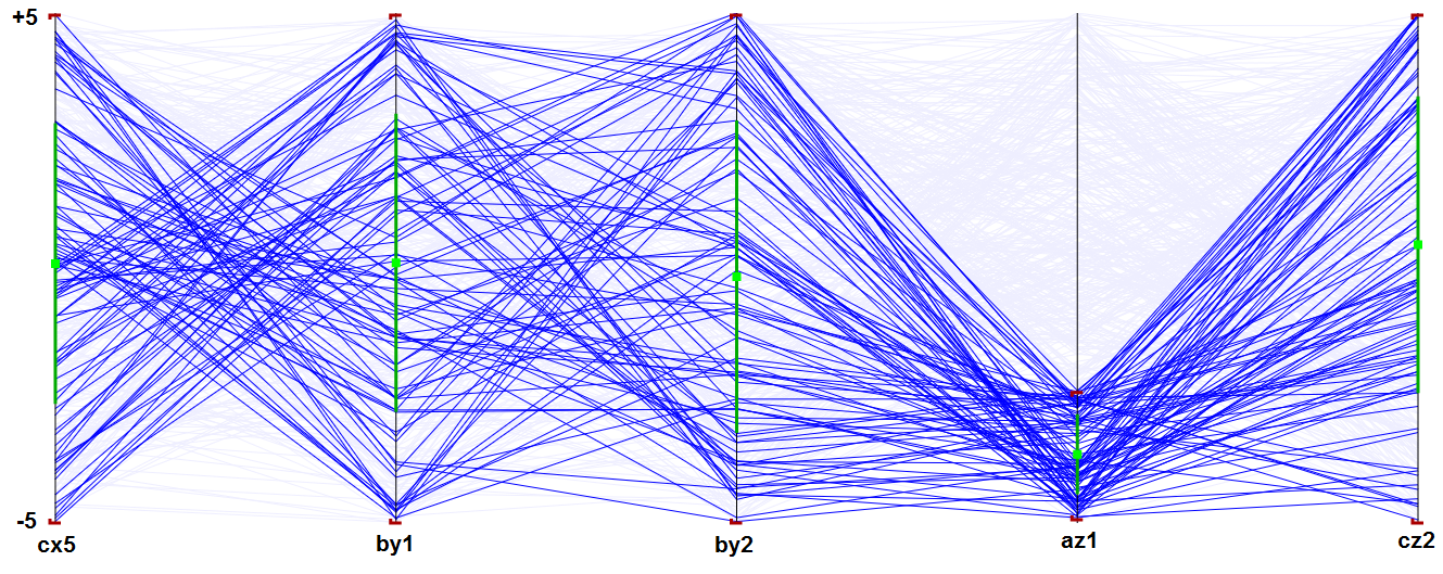
Figure 2 shows an example of chaotic sample points generated from the equations of Case N in Table I of Sprott [18]. The general system in Sprott [18] is given as:

$$\frac{dx}{dt} =a_{x1}+b_{x1}x+b_{x2}y+b_{x3}z+c_{x1}x^{2}+c_{x2}xy+c_{x3}xz+c_{x4}y^{2}+c_{x5}yz+c_{x6}z^{2}$$

$$\frac{dy}{dt} =a_{y1}+b_{y1}x+b_{y2}y+b_{y3}z+c_{y1}x^{2}+c_{y2}xy+c_{y3}xz+c_{y4}y^{2}+c_{y5}yz+c_{y6}z^{2}$$

$$\frac{dz}{dt} =a_{z1}+b_{z1}x+b_{z2}y+b_{z3}z+c_{z1}x^{2}+c_{z2}xy+c_{z3}xz+c_{z4}y^{2}+c_{z5}yz+c_{z6}z^{2}$$

The 5 parameters we varied are $c_{x5}$, $b_{y1}$, $b_{y2}$, $a_{z1}$ and $c_{z2}$; the remainder of the parameters were chosen to be zero. Each of the selected varied parameters is mapped to an individual coordinate axis, arranged in parallel from left to right, with each sample point drawn as a “poly line” that intersects each coordinate axis at the appropriate location. All five parameters were constrained to lie in the interval $[-5,5]$ during initial sampling, although by dynamically dragging the upper and lower endpoint markers on each axis, the user can further restrict the display so it only shows samples generated within a smaller sub-rectangle. Here, we have decreased the upper bound on the parameter $a_{z1}$ to $-2.4$, filtering out some of the $500$ initial sample points initially present.

Figure 3: The result (from left to right) of dragging down the upper limit on the $c_{x5}$ axis, observing a corresponding increase in the mean of the $b_{y1}$ axis due to anticorrelation between the two.

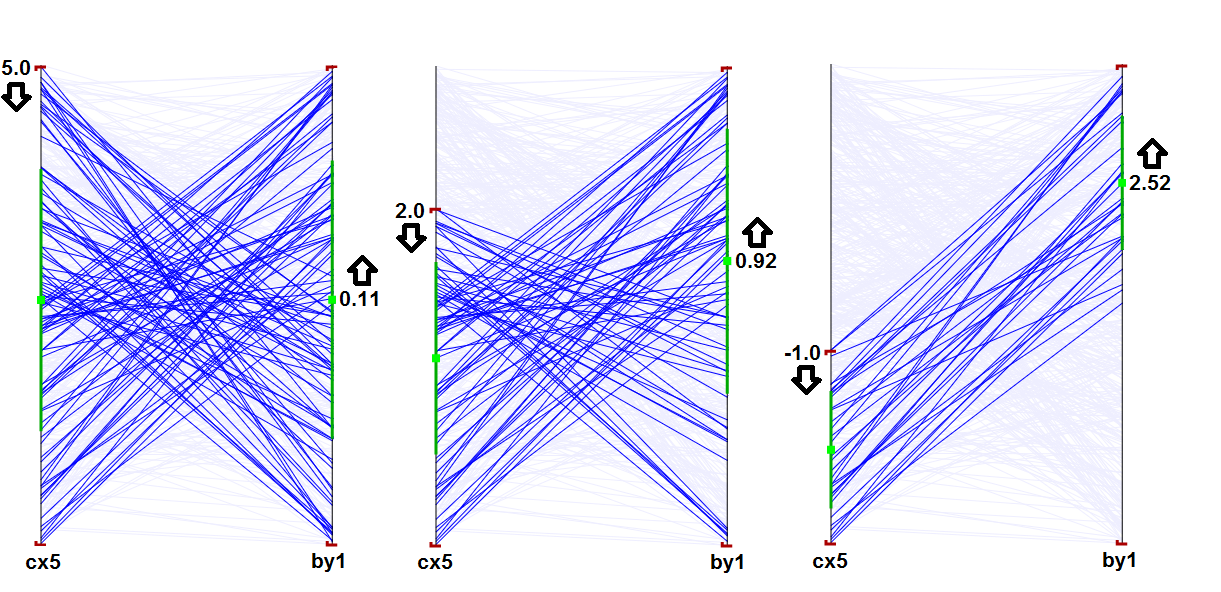
Parallel coordinate plots allow us to understand a number of useful properties by visual inspection and interactive manipulation. For example, in Figure 2, we see that in order to achieve chaos with $a_{z1}$ restricted to such a low range, the parameters $c_{x5}$ and $b_{y1}$ need to be anticorrelated: that is, there needs to be a negative relationship in which $c_{x5}$ increases as $b_{y1}$ decreases. This is visually apparent from the “X” pattern between the $c_{x5}$ and $b_{y1}$ axes, and we can also see it by dynamically dragging the upper bound on $c_{x5}$ downward, watching the marker for the mean value on the $b_{y1}$ axis move upward in lock step, as shown in Figure 3. Interestingly, if one raises the lower bound on $a_{z1}$, forcing this parameter to take large values, then the pattern between $c_{x5}$ and $b_{y1}$ becomes one of mostly straight horizontal lines, indicating correlation rather than anticorrelation.

By restricting several coordinates at a time, the user can filter an initially large number of sample points down to only a few. For example, if we restrict the range to half of each of five axes, this will on average show only $1/2^{5}$ of all our sample points. In order to populate the filtered space with sufficiently many samples to understand its geometric structure, it may be necessary to re-launch a new round of MH sampling within this restricted space, requiring tight coupling between the user interface and the “back end” parallel MH sampler.

3 Numerical Results

As the main goal of our work is to provide researchers with a convenient numerical method for exploring chaotic behavior of their systems of interest, we tested the ability of our algorithm to find parameter settings leading to chaotic states using three systems from literature. We use this section to describe those systems and provide the associated numerical results. At the end of every example we make observations on the combinations of parameters and initial values that lead to chaos as examples of the type of information that researchers studying such systems will be able to derive using our methods without rigorous mathematical study.

We begin with the system presented by Kot et al. [12], where the authors analyze a forced double-Monod model in an initial effort to understand chaos in biological systems. We next consider a system of equations for modeling plant growth in the rhizosphere (Kravchenko et al. [14], Strigul and Kravchenko [20]), which includes multiple prey species, a predator species, and a nutrient source. Finally, we use our framework to analyze a system of equations motivated by experimental measurements of a bacterial population with a nutrient source (Becks et al. [4]).

3.1 Double forced Monod system

We first consider one of the dynamical systems presented and analyzed in work by Kot, Sayler, and Schultz [12]. While experimental results are not included in the paper, the authors justify their choice to study this particular system by noting the possibility of obtaining experimental validation of their work. As our primary interest in developing the framework presented here is to aid biologists in their data-based studies of dynamical systems, this particular problem presents an ideal benchmark case.

The dimensionalized equations are given as

$$\frac{dS}{dt} =D\left[S_{i}\left(1+\epsilon\sin\left(\frac{2\pi}{T}t\right)\right)-S\right]-\frac{\mu_{1}}{Y_{1}}\frac{SH}{K_{1}+S}$$

$$\frac{dH}{dt} =\mu_{1}\frac{SH}{K_{1}+S}-DH-\frac{\mu_{2}}{Y_{2}}\frac{HP}{K_{2}+H}$$

$$\frac{dP}{dt} =\mu_{2}\frac{HP}{K_{2}+H}-DP,$$

where $S$ represents the limiting substrate, $H$ represents a prey species, and $P$ represents a predator species. We note the predator species consumes only the prey, so its population is indirectly associated with the changes in $S$. The parameters in the model govern the response of the organisms to changes in the system. $D$ is the dilution rate, which defines the ratio of the flow into the chemostat to the volume of organisms in the chemostat; $\mu_{1}$ and $\mu_{2}$ are the maximum specific growth rates of the prey and predator, respectively; $Y_{1}$ is the yield of prey per unit mass of substrate, and $Y_{2}$ is the yield of predator per unit mass of prey; and $K_{1}$ and $K_{2}$ are the half-saturation constants. $S_{i}$ is the inflowing substrate concentration.

The equations are nondimensionalized by rescaling all variables by the inflow substrate, the prey by its yield constant $Y_{1}$, and the predator by both yield constants (Kot et al. [12]). The dimensionless system is given by

$$\frac{dx}{d\tau} =1+\epsilon\sin\left(\omega\tau\right)-x-\frac{Axy}{a+x}$$

$$\frac{dy}{d\tau} =\frac{Axy}{a+x}-y-\frac{Byz}{b+y}$$

$$\frac{dz}{d\tau} =\frac{Byz}{b+y}-z,$$

where $x=\displaystyle\frac{S}{S_{i}}$, $y=\displaystyle\frac{H}{Y_{1}S_{i}}$, and $z=\displaystyle\frac{P}{Y_{1}Y_{2}S_{i}}$, $\tau=Dt$, and $\omega=\displaystyle\frac{2\pi}{DT}$. Also, $A=\displaystyle\frac{\mu_{1}}{D}$, $a=\displaystyle\frac{K_{1}}{S_{i}}$, $B=\displaystyle\frac{\mu_{2}}{D}$, and $b=\displaystyle\frac{K_{2}}{Y_{1}S_{i}}$.

The dimensionless system exhibits chaotic behavior for $\omega=\displaystyle\frac{5\pi}{6}$ and $\epsilon=0.6$, with $S_{i}=115$ mg/l, $D=0.1$ / h, and initial conditions $x=0.42\text{, }y=0.4\text{, }z=0.42$. The remainder of the parameter values are provided in Table 1. Representative manifold plots are given in Kot et al. [12] and are not duplicated here.

	$Y_{i}$	$\mu_{i}$ h-1	$K_{i}$ mg/l
Prey ($i=1$)	0.4	0.5	8
Predator ($i=2$)	0.6	0.2	9

Table 1: Parameter values associated with the chaotic system described in Kot et al. [12].

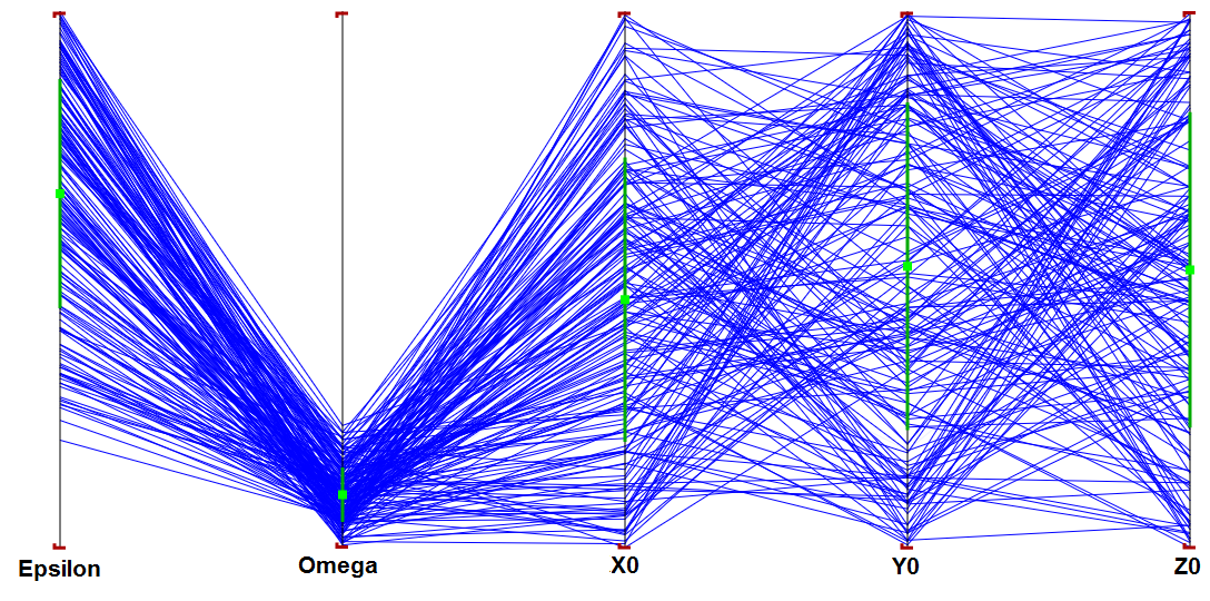
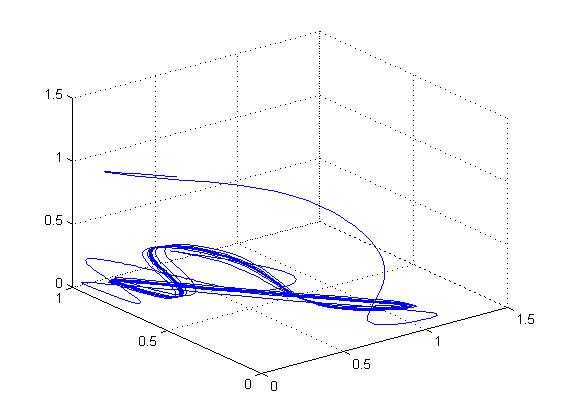
We wanted to replicate the findings in Kot et al. [12] in order to confirm that our framework can identify parameter values leading to chaotic and non-chaotic states. The authors Kot et al. [12] noted that particular values of $\omega$ and $\epsilon$ were associated with chaotic states, so we chose to search over ranges of these two parameters, along with ranges for the initial conditions for the system. A subset of our results is shown using the parallel coordinates visualization in Figure 4. This visualization indicates more positive Lyapunov exponents associated with small values of $\omega$. Notice that in the rescaled system $\omega$ is the angular frequency of the forcing term. Observing positive Lyapunov exponents for small values of $\omega$ may indicate to a biologist an interesting connection between periodic forcing and chaotic behavior that they may be able to further study experimentally. Any clustering of the remainder of the parameters chosen for our study is less obvious. Figure 5 contains a manifold plot of the dimensionless system for a randomly chosen set of parameter values $\epsilon=0.4809$, $\omega=1.9109$, and initial conditions $x(0)=0.3878$, $y(0)=0.7866$, and $z(0)=0.8875$. This parameter set returned a positive Lyapunov exponent. We note that the strange attractor is distinct from the one given in the referenced paper.

Figure 4: Results from the parameter search for the double forced Monod system in Kot et al. [12] visualized using parallel coordinates. The vertical axes are associated with values for $\epsilon$, $\omega$, $x(0)$, $y(0)$, and $z(0)$, and the maximum calculated Lyapunov exponent.

Figure 5: Manifold plot of forced model in Kot et al. [12]. Note the strange attractor is distinct from the one given in the paper.

3.2 Models of rhizozone bacteria

Our second example system is motivated by studies of bacterial growth in the rhizosphere. In particular, we consider the models for plant growth promoting rhizobactera (PGPR) inoculation developed by Kravchenko, Strigul, and Shvytov [14] and Strigul and Kravchenko [20]. In those works, the authors developed the following model equations to describe the dynamics of their two prey, one predator system with a periodic nutrient source:

$$\frac{dX}{dt} =X\left(\mu_{X}\left[S,P,N\right]+F\left[Z\right]-\alpha X-d_{1}\right)$$

$$\frac{dZ}{dt} =Z\left(\mu_{z}\left[S,P,N\right]+G\left[X\right]-\beta Z-d_{2}\right)$$

$$\frac{dS}{dt} =W\left(t\right)+L-D_{S}\left(S-S_{0}\right)-\frac{X\mu_{x}\left[S,P,N\right]}{Y_{XS}}-\frac{Z\mu_{z}\left[S,P,N\right]}{Y_{ZS}}$$

$$\frac{dP}{dt} =D_{P}\left(P_{0}-P\right)-\frac{X\mu_{x}\left[S,P,N\right]}{Y_{XP}}-\frac{Z\mu_{z}\left[S,P,N\right]}{Y_{ZP}}$$

In this system, $X$ and $Z$ represent the concentration of PGPR and resident micro-organisms, respectively, $S$ represents an organic substrate concentration, and $P$ represents the concentration of oxygen in the soil (Strigul and Kravchenko [20]). The parameters $\mu_{X}$ and $\mu_{Z}$ are growth rates dependent on the available substrate $S$, oxygen $P$, and nitrogen $N$ through defined growth rate functions. These functions are rate limited and have the general form

$$\mu_{*}\left[S,P,N\right]=\mu_{m*}\frac{S}{S+\theta K_{S*}}\frac{P}{P+K_{P*}}\frac{N}{N+\theta K_{N*}},$$

where $\mu_{m*}$ is a specified maximal growth rate for the species of interest, $\theta$ is the moisture content of the soil, and $K_{S*}$ represents an affinity constant for the species to the organic substrate. The constants $K_{N*}$ and $K_{P*}$ are similarly defined. The initial values of the parameters used in our work are provided in detail in Strigul and Kravchenko [20].

The function $W(t)$ is meant to simulate the effects of photosynthesis, and is therefore periodic with period length $24$ h. We incorporate this into our model system using a Fourier series expansion of the piecewise constant function

$$f(x)=\left\{\begin{array}[]{rl}1,&0<x\leq 12\\ 0,&12<x<24.\end{array}\right.$$

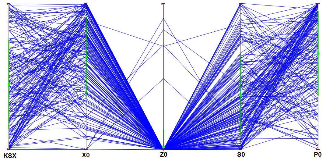
Mathematical analysis of the PGPR models was not provided in the papers we considered (Kravchenko et al. [14], Strigul and Kravchenko [20]). However, the authors of those works indicate that rigorous analysis of the system should prove the existence of chaotic states. In addition, as the characteristics of the PGPR models are similar to other dynamical systems known to exhibit chaotic behavior, we believe this to be a reasonable system for further evaluation of our framework. Towards that end, we use our algorithm to search over ranges of $K_{SX}$ and ranges of initial values for $X$, $Z$, $S$, and $P$. A subset of the results we obtain is shown in the parallel coordinates plot in Figure 6. We note the definite clustering of values for the parameters. In particular, we note the value of $Z(0)$ is almost uniformly on the lower end of the selected search range. Such a finding would facilitate a researcher interested in studying (or avoiding) chaotic behavior of their system by clearly pointing to the low values to which $Z(0)$ should (not) be set.

Figure 6: A parallel coordinates plot for a subset of the results for the the PGPR models in Strigul and Kravchenko [20]. The vertical axes are associated with values of $K_{SX}$, $X(0)$, $Z(0)$, $S(0)$, and $P(0)$, along with the associated maximum Lyapunov exponent.

3.3 Models for experimental data

For the third example, we model a set of experimental data where chaotic states were demonstrated for varying levels of the dilution parameter (Becks et al. [4]). The authors of that work describe experimental scenarios where the system under study could transition from chaotic to equilibrium states, and vice versa, by crossing a threshold value for the dilution rate.

Our approach for modeling the data uses a set of rate-limited, dynamical equations similar to those in the previous examples. The model equations and system parameters were estimated by in Molz and Faybishenko [16]. Their intent was to derive a mathematical model whose dynamics closely resembled the experimental dynamics seen in Becks et al. [4]. The general description of the system we consider is given by

$$\begin{aligned} \frac{dR}{dt}&=R\left[\mu_{NR}\left(\frac{N}{K_{NR}+N}\right)-\delta_{R}\right]-\frac{\mu_{PR}}{Y_{PR}}\left(\frac{R}{K_{PR}+R}\right)P-DR\\ \frac{dC}{dt}&=C\left[\mu_{NC}\left(\frac{N}{K_{NC}+N}\right)-\delta_{C}\right]-\frac{\mu_{PC}}{Y_{PC}}\left(\frac{C}{K_{PC}+C}\right)P-DC\\ \frac{dP}{dt}&=P\left[\mu_{PR}\left(\frac{R}{K_{PR}+R}\right)+\mu_{PC}\left(\frac{C}{K_{PC}+C}\right)-\delta_{P}\right]-DP\\ \frac{dN}{dt}&=DN_{0}-R\left[\frac{\mu_{NR}}{Y_{NR}}\left(\frac{N}{K_{NR}+N}\right)\right]-C\left[\frac{\mu_{NC}}{Y_{NC}}\left(\frac{N}{K_{NC}+N}\right)\right]-DN.\end{aligned}$$ (1)

The variables $R$ and $C$ represent the prey species of rods and cocci, respectively. We let $P$ represent the prey species, and $N$ represents a nutrient source to the system. The parameter $D$ represents the dilution rate for input of nutrients to the system.

The parameters in the model determine the feeding habits of the predator and prey, as well as death and growth rates for each species. These parameters may be used to specify particular behaviors of the organisms, e.g., growth rates due to feeding on nutrient sources rather than prey. We define $\mu_{N*}$ as maximum growth rates for the associated species based on consumption of nutrients and $\mu_{P*}$ as the maximum growth rates for predator based on consumption of the associated prey species. The value of $K_{N*}$ is the half saturation constant for the species on the nutrient, and $K_{P*}$ is the half saturation constant for the predator on the associated species. Note that these latter constants may determine a “preference” for one prey over the other. The parameters $Y_{N*}$ represent yield coefficients for the species on the nutrient, and $Y_{P*}$ represents the yield coefficients for the predator associated with the prey species. Death rates for each species are given by $\delta_{*}$. We provide specific values we used for these parameters in Table 2.

	Species
Parameter	R	C	P
$\mu_{N*}$	12 / day	6 / day
$\mu_{P*}$	2.2 / day	2.2 / day
$K_{N*}$	8e-6 gm/cc	8e-6 gm/cc
$K_{P*}$	1e-6 gm/cc	1e-6 gm/cc
$Y_{N*}$	0.1 gm R / gm N	0.1 gm C / gm N
$Y_{P*}$	0.12 gm P / gm R	0.12 gm P / gm C
$\delta_{*}$	0.5 / day	0.25 / day	0.08 / day

Table 2: Parameter values for model equations (1) used in the numerical simulations.

The model incorporates fifteen parameters. The parameter space can be reduced by rescaling the state variables $R$, $C$, $P$ and $N$, and time $T$. Rescaling the equations eliminates four of the parameters and simultaneously makes the system more perspicuous for both qualitative analysis and numerical simulation. We chose to rescale by introducing the following change of variables

$$R =K_{PR}\,r,\quad C=K_{PC}\,c,\quad P=\dfrac{K_{PR}Y_{PR}\left(\delta_{R}+D\right)}{\mu_{PR}}\,p,$$

$$N =K_{NR}\,n,\quad T=\dfrac{1}{\delta_{R}+D}\,t,$$

where the lowercase $r$, $c$, $p$, $n$ and $t$ are the new rescaled variables and time, respectively. The rescaled model equations are given by

$$\begin{aligned} \frac{dr}{dt}&=\widehat{\mu}_{NR}\left(\frac{nr}{n+1}\right)-\left(\frac{rp}{r+1}\right)-r\\ \frac{dc}{dt}&=\widehat{\mu}_{NC}\left(\frac{nc}{n+\widehat{\kappa}}\right)-\widehat{\eta}_{1}\left(\frac{cp}{c+1}\right)-\widehat{\delta}_{C}\,c\\ \frac{dp}{dt}&=\widehat{\mu}_{PR}\left(\frac{rp}{r+1}\right)+\widehat{\mu}_{PC}\left(\frac{cp}{c+1}\right)-\widehat{\delta}_{P}\,p\\ \frac{dn}{dt}&=\widehat{\delta}\left(n_{0}-n\right)-\widehat{\eta}_{2}\left(\frac{nr}{n+1}\right)-\widehat{\eta}_{3}\left(\frac{nc}{n+\widehat{\kappa}}\right),\end{aligned}$$ (2)

where the new (eleven) parameters are expressed in terms of the original parameters as follows:

$$\widehat{\mu}_{NR} =\dfrac{\mu_{NR}}{\left(\delta_{R}+D\right)},\quad\widehat{\mu}_{NC}=\dfrac{\mu_{NC}}{\left(\delta_{R}+D\right)},$$

$$\widehat{\mu}_{PR} =\dfrac{\mu_{PR}}{\left(\delta_{R}+D\right)},\quad\widehat{\mu}_{PC}=\dfrac{\mu_{PC}}{\left(\delta_{R}+D\right)},$$

$$\widehat{\kappa}=\dfrac{K_{NC}}{K_{NR}},\,\widehat{\delta}_{C} =\dfrac{\delta_{C}+D}{\left(\delta_{R}+D\right)},\,\widehat{\delta}_{P}=\dfrac{\delta_{P}+D}{\left(\delta_{R}+D\right)},\,\widehat{\delta}=\dfrac{D}{\left(\delta_{R}+D\right)},$$

$$\widehat{\eta}_{1}=\dfrac{\mu_{PC}Y_{PR}K_{PR}}{\mu_{PR}Y_{PC}K_{PC}},\,\widehat{\eta}_{2} =\dfrac{\mu_{NR}K_{PR}}{Y_{NR}K_{NR}\left(\delta_{R}+D\right)},\,\widehat{\eta}_{3}=\dfrac{\mu_{NC}K_{PC}}{Y_{NC}K_{NR}\left(\delta_{R}+D\right)}.$$

We also introduce the initial value for the rescaled nutrient source, $n_{0}=K_{NR}N_{0}$.

We studied the dynamics of our proposed model by examining the effects of changes in the dilution rate $D$ and the initial nutrient concentration $N(0)$. These are logical choices as the authors Becks et al. [4] associated the chaotic states with the value of the dilution rate. Our previous work led us to choose the initial nutrient concentration as well, as non-steady access to resources can affect the overall behavior of the system. We calculated the maximum Lyapunov exponent for the system using $D$ in the range $[0.3,2]$ and $N(0)$ in the range $[0.1,1]$, and found that it was positive across this entire range.

Figure 7 contains parallel coordinates plots generated using ranges of values for $D$, $N(0)$, and the corresponding maximum Lyapunov exponent of each sample point. By including maximum Lyapunov exponent in these plots, we see that there is a small “island” of sample points that behaves qualitatively differently from the rest; when we isolate these points by increasing the lower bound on maximum Lyapunov exponent, we see that they come from a very specific range of values in terms of $D$ and $N(0)$.

Figure 7: Parallel coordinates plots of $D$, $N(0)$, and maximum Lyapunov exponent (MLE). The plot on the right shows the result of dragging the lower bound on MLE upward to isolate only sample points with large MLE.

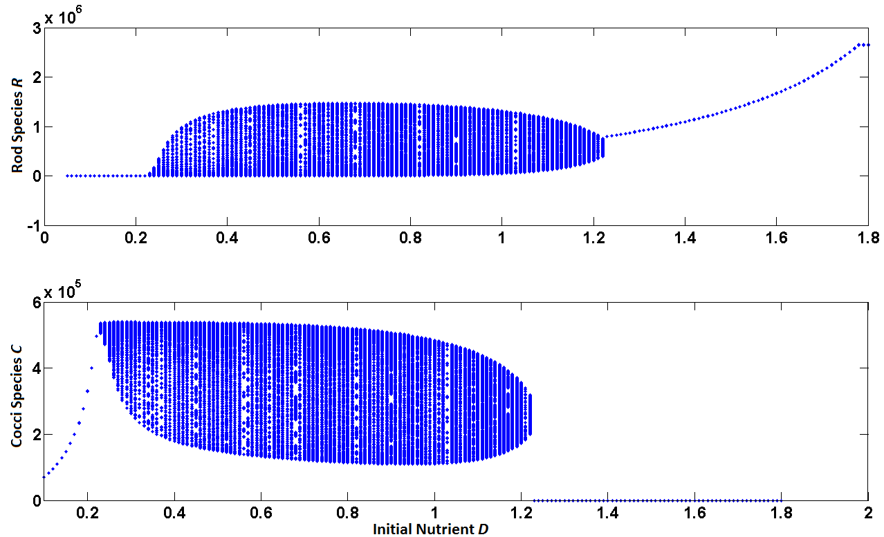
We also generated bifurcation graphs associated with this system of equations using the dimensionalized equations and varying the dilution rate $D$. These are shown in Figure 8. The plots were generated using the MATLAB ode45 ODE integrator and plotting tools. The system was solved over the time frame $t\in[0,7500]$ for each choice of $D$. The plot contains the solutions computed for the two prey species, $R$ and $C$, versus $D$ for $t\in[7000,7500]$ using 500 evenly spaced points. We see evidence of chaotic behavior for $D\in[0.2,1.2]$.

Figure 8: Bifurcation plot of the ODE system showing the solutions for $R$ and $C$ versus $D$. Note the effect of the changing dilution rate.

4 Conclusions

We have provided a framework that allows researchers to efficiently search over a design space including parameter values and initial conditions and discover possible connections between values of these constants and chaotic dynamics. The ability for such a search may reveal chaotic behavior in systems not previously known to have chaotic regime and reveal the existence of parameters and initial conditions not previously known to yield chaotic behavior in studied systems. We described a software framework for those wishing to analyze systems for chaotic dynamics without the need for rigorous mathematical analysis. One of its main strengths is allowing for studying system behavior that is virtually impossible to observe in laboratory environment, thus making it useful to experimentalists. The parallel coordinate plots further provide insight into understanding system dynamics for a wide variety of parameter changes.

Our algorithms can be further optimized. One obvious direction is to investigate further methods of parallelizing the environment, which would significantly speed up the computations.

References

- Banks [1975] H.T. Banks. Modeling and Control in the Biomedical Sciences, volume 6 of Lecture Notes in Biomathematics. Springer-Verlag, Heidelberg, 1975.
- Banks and Davidian [2009] H.T. Banks and M. Davidian. Introduction to the chemostat. http://www.ncsu.edu/crsc/htbanks/STMA810c/chemostat.pdf, 2009.
- Becks and Arndt [2008] L. Becks and H. Arndt. Transitions from stable equilibria to chaos, and back, in an experimental food web. Ecology, 89:3222–3226, 2008.
- Becks et al. [2005] L. Becks, F.M. Hilker, H. Malchow, K. Jürgens, and H. Arndt. Experimental demonstration of chaos in a microbial food web. Nature, 435:1226–1229, June 2005.
- Benettin et al. [1980] G. Benettin, L. Galgani, A. Giorgilli, and J.-M. Strelcyn. Lyapunov characteristic exponents for smooth dynamical systems and for Hamiltonian systems: a method for computing all of them. Meccanica, 15(1):21–30, 1980.
- Costantino et al. [1997] R. Costantino, R. Desharnais, J. Cushing, and B. Dennis. Chaotic dynamics in an insect population. Science, 275:389–391, 1997.
- Dennis et al. [1997] B. Dennis, R. Desharnais, J. Cushing, and R. Costantino. Transitions in population dynamics: equilibria to periodic cycles to aperiodic cycles. J. Anim. Ecol., 66:704–729, 1997.
- Fussmann et al. [2000] G. Fussmann, S. Ellner, K. Shertzer, and N. Hairston. Crossing the Hopf bifurcation in a live predator-prey system. Science, 290:1358–1360, 2000.
- Henson [2003] M.A. Henson. Dynamic modeling of microbial cell populations. Curr. Opin. Biotech., 14:460–467, 2003.
- Jost et al. [1973] J. Jost, J. Drake, A. Frederickson, and H. Tsuchiya. Interactions of Tetrahymena pyrifarmis, Escherichia coli, Azobacter vinelndil, and glucose in a mineral medium. J. Bacteriol, 113:834–840, 1973.
- Kooi and Boer [2003] B.W. Kooi and M.P. Boer. Chaotic behavior of a predator-prey system in the chemostat. Dynam. Cont. Dis. Ser. B, 10(2):259–272, 2003.
- Kot et al. [1992] M. Kot, G.S. Sayler, and T.W. Schultz. Complex dynamics in a model microbial system. B. Math. Biol., 54(4):619–648, 1992.
- Kovárová-Kovar and Egli [1998] K. Kovárová-Kovar and T. Egli. Growth kinetics of suspended microbial cells: From single-substrate-controlled growth to mixed-substrate kinetics. Microbiol. Mol. Biol. R., 62(3):646–666, 1998.
- Kravchenko et al. [2004] L.V. Kravchenko, N.S. Strigul, and I.A. Shvytov. Mathematical simulation of the dynamics of interacting populations of rhizosphere microorganisms. Microbiology, 73(2):189–195, 2004.
- Michaelis and Menten [1913] L. Michaelis and M.L. Menten. Die kinetik der invertinwirkung. Biochemistry Z, 49:333–369, 1913.
- Molz and Faybishenko [2013] F. Molz and B. Faybishenko. Increasing evidence for chaotic dynamics in the soil-plant-atmosphere system: A motivation for future research. Procedia Environmental Sciences, 19:681–690, 2013.
- Shimada and Nagashima [1979] L. Shimada and T. Nagashima. A numerical approach to erogodic problem of dissipative dynamical systems. Prog. Theor. Phys., 61(6):1605–1616, 1979.
- Sprott [1994] J.C. Sprott. Some simple chaotic flows. Phys. Rev. E, 50(2):647–650, 1994.
- Sprott [2003] J.C. Sprott. Chaos and Time-Series Analysis. Oxford University Press, Oxford, UK, 2003.
- Strigul and Kravchenko [2006] N.S. Strigul and L.V. Kravchenko. Mathematical modeling of PGPR inoculation into the rhizosphere. Environ. Modell. Softw., 21:1158–1171, 2006.
- Wolf et al. [1985] A. Wolf, J.B. Swift, H.L. Swinney, and J.A. Vastano. Determining Lyapunov exponents from a time series. Physica, pages 285–317, 1985.