SEMICLASSICAL APPROACHES TO NUCLEAR DYNAMICS

Abstract

The extended Gutzwiller trajectory approach is presented for the semiclassical description of nuclear collective dynamics, in line with the main topics of the fruitful activity of V.G. Solovjov. Within the Fermi-liquid droplet model, the leptodermous effective-surface approximation was applied to calculations of energies, sum rules and transition densities for the neutron-proton asymmetry of the isovector giant-dipole resonance and found to be in good agreement with the experimental data. By using the Strutinsky shell-correction method, the semiclassical collective transport coefficients such as nuclear inertia, friction, stiffness, and moments of inertia can be derived beyond the quantum perturbation approximation of the response-function theory and the cranking model. The averaged particle-number dependence of the low-lying collective vibrational states are described in good agreement with basic experimental data, mainly due to an enhancement of the collective inertia as compared to its irrotational flow value. Shell components of the moment of inertia are derived in terms of the periodic-orbit free-energy shell corrections. A good agreement between the semiclassical extended Thomas-Fermi moments of inertia with shell corrections and the quantum results is obtained for different nuclear deformations and particle numbers. Shell effects are shown to be exponentially dampted out with increasing temperature in all the transport coefficients.

I INTRODUCTION

Many experimental data on the fundamental properties of fission, and collective excitations in nuclei, were successfully explained by using the macroscopic-microscopic approaches to the description of finite Fermi systems with strongly interacting nucleons migdal ; strut ; myswann69 ; fuhi ; fraupash ; bormot ; mix ; belyaevzel ; SOLbook1981 ; SOLbook1992 ; hofbook . One of the transparent and, at the same time, fruitful ways to study collective excitations in complex nuclei was suggested by V.G. Solovjov and his collaborators within the semi-microscopic Quasiparticle-Phonon Model (QPM) SOLbook1981 ; SOLbook1992 ; SOLQPMI-EPNP1978 ; SOLQPMII-EPNP1980 ; SOLQPMIII-EPNP1983 ; SOLQPMIV-EPNP1983 ; SOLQPMV-EPNP1985 . We should also mention the theoretical mean-field approaches, based in particular on the cranking model bormot ; inglis ; bohrmotpr ; valat . By using the cranking model and the Strutinsky shell-correction method (SCM) strut ; fuhi ; fraupash , shell effects in the vibrational and rotational bands were intensively studied migdal ; bormot ; mix . These approaches are rooted in the self-consistent finite-Fermi-system theory migdal ; khodsap and its mean-field Hartree-Fock (HF) brink and HF-Bogoliubov (HFB) solovjov1 ; ringschuck ; brackquenNPA1981 approximations. For small-amplitude collective excitations they are equivalent to the Random Phase Approximation (RPA) of the QPM. However, the HF and HFB approaches go beyond the RPA since they can be applied for large-amplitude collective motion as well. Concerning all these approaches, we should also mention pairing correlations SOLsuperfluidity-NPA1958 ; belyaev61 ; SOLbook1963 ; belzel ; belsmitolfay87 , and high spins physics (see sfraurev for a review). The problem of the coexistence of oblate-prolate shapes in relation to rotational bands was discussed in matmatnak2010_12 ; hinsatnak2010_11 .

For the description of nuclear collective excitations within the general response-function theory bormot ; hofbook , which can be associated with the RPA of the QPM, the basic idea is to parametrize the complex dynamical problem of the collective motion of many strongly interacting particles in terms of a few main collective variables found from the physical meaning of the considered dynamical problem, for example the nuclear surface itself strtyap ; strmagbr ; strmagden or its multipole deformations bormot ; solovjov1 . We can then study the response of the dynamical quantities, describing the nuclear collective motion in terms of these variables, to an external field. Thus, we get important information on the transport properties of nuclei. For such a theoretical description of the collective motion it is often very important to take into account the temperature dependence of the dissipative nuclear characteristics as the friction coefficient, as shown in hofbook ; hofivyam ; hofmann ; ivhofpasyam .

However, a precise quantum description of dissipative phenomena in nuclei is rather complicated because one has to take into account the residual interaction beyond the mean-field approximation. Therefore, a simpler Fermi-liquid drop model (FLDM) kolmagpl ; magkohofsh ; kolmagsh ; belyaev accounting for some macroscopic properties of the many-body Fermi system can be helpful to understand the global average properties of the collective motion. Such a model is based on the Landau Fermi-liquid theory landau ; abrikha ; pinenoz ; baympeth , applied for the nuclear interior and some simple macroscopic boundary conditions on the nuclear surface strmagbr ; strmagden ; kolmagsh ; magstr ; magboundcond . An extension of the effective-surface method strtyap ; strmagbr ; strmagden to neutron-proton systems, that is accounting for the asymmetry, spin-orbit and Swiatecki’s derivative terms in the local energy-density approach rungegrossPRL1984 ; marquesgrossARPC2004 is given in magsangzh ; BMRV ; BMRPhysScr2014 ; BMRps2015 ; BMRprc2015 . A more extensive discussion of other macroscopic approaches, in particular with different boundary conditions can be found in the review belyaev . In magkohofsh , the response-function theory was applied to describe collective nuclear excitations as the isoscalar quadrupole mode. The transport coefficients, such as friction and inertia, are simply calculated within the macroscopic FLDM, and their temperature dependence can be easily discussed magkohofsh ; kolmagsh ; belyaev . The isospin asymmetry of heavy nuclei near their stability line and the structure of the isovector dipole resonance are studied within the FLDM kolmagsh ; belyaev ; BMRV ; BMRPhysScr2014 ; BMRps2015 ; BMRprc2015 ; kolmag . In this way, the giant multipole resonances were described, in particular, by taking into account a gradual transition with increasing temperature from a zero sound mode to the hydrodynamic first sound kolmagpl ; magkohofsh ; belyaev . The friction phenomenon is described in kolmagpl ; magkohofsh as being due to nucleon-nucleon collisions, which were taken into account in the relaxation-time approximation (see e.g. abrikha ; pinenoz ; baympeth for a general description, and kolmagpl ; belyaev for a specific account of a temperature and frequency dependence (retardation effects)) kolmagpl ; belyaev ; landau . Relations to some general problems of the response-function theory hofbook and their understanding, taking the example of an analytically solved model based on a nontrivial temperature-dependent Fermi-liquid theory, can be found in belyaev . One of the most important questions which was clarified there is the temperature dependence of friction and interaction-coupling constants.

Within this extended macroscopic (FLDM) theory, one can determine the structure of the isovector dipole resonance (IVDR) as a splitting of the collective states due to the nuclear symmetry interaction between neutrons and protons near the stability line kolmagsh ; belyaev ; BMRV ; BMRPhysScr2014 ; BMRps2015 ; BMRprc2015 ; kolmag . Also, the neutron skin of exotic nuclei with a large neutron excess is still one of the exciting subjects of nuclear physics and nuclear astrophysics myswann69 ; myswnp80pr96 ; myswprc77 ; myswiat85 ; danielewicz1 ; pearson ; danielewicz2 ; vinas1 ; vinas2 ; vinas3 ; vinas4 ; vinas5 . Simple and accurate solutions for the isovector particle density distributions were obtained within the nuclear effective-surface (ES) approximation strtyap ; strmagbr ; strmagden ; magsangzh ; BMRV ; BMRPhysScr2014 ; BMRps2015 ; BMRprc2015 which exploits the saturation property of nuclear matter and a narrow diffuse-edge region in finite heavy nuclei. In particular, in the Extended Thomas–Fermi (ETF) approach brguehak ; sclbook (with Skyrme forces chaban ; reinhard ; reinhardSV ; jmeyer ; bender ; revstonerein ; ehnazarrrein ; pastore ) this can be done for any deformation by using an expansion in a small leptodermic parameter. The latter can be defined as the diffuse surface thickness of a heavy nucleus relative to its mean curvature radius, proportional to $A^{-1/3}$, where $A$ is the nuclear particle number. For deformed nuclear shapes such an approach can be carried through under the constraint on some multipole moments. The accuracy of the ES approximation in the ETF approach without the spin-orbit (SO) and asymmetry terms was checked strmagden by comparing with the results of the HF brink ; ringschuck and ETF calculations brguehak ; sclbook for different Skyrme forces. The ES approach strtyap ; strmagbr ; strmagden was then extended by taking the SO interaction, and asymmetry effects into account magsangzh ; BMRV ; BMRPhysScr2014 ; BMRps2015 ; BMRprc2015 . Solutions for the isoscalar and isovector particle densities and energies at the quasi-equilibrium in the ES approach of the ETF approach were applied to analytical calculations of the neutron skin and isovector stiffness coefficients in leading order of the leptodermic parameter and to the derivations of the macroscopic boundary conditions strtyap ; strmagbr ; strmagden ; magsangzh ; BMRV ; BMRprc2015 and compared with those obtained in the liquid droplet model (LDM) myswann69 ; myswnp80pr96 ; myswprc77 ; myswiat85 . These analytical expressions for the surface-energy constants can also be used for IVDR calculations within the FLDM (see belyaev and references therein).

A further interesting application of the semiclassical response-function theory would consist in the study of the properties of collective transport phenomena, in particular the low-lying excitations and rotational bands in heavy deformed nuclei. One may consider nuclear collective rotations within the cranking model as a response of the nuclear system to the Coriolis external-field perturbation. The moment of inertia (MI) can be calculated as a kind of susceptibility with respect to this external field. The rotation frequency of the rotating Fermi system is determined in the cranking model for a given nuclear angular momentum through a constraint, as for any other integral of motion, as in particular the particle number conservation ringschuck . In order to simplify such a rather complicated problem, the Strutinsky shell correction method (SCM) strut ; fuhi was adjusted to the collective nuclear rotations in mix ; fraupash . The collective MI is expressed as function of the particle number and temperature in terms of a smooth part and an oscillating shell correction. The smooth component can be described by a suitable semiclassical macroscopic model, like the dynamical ETF approach brguehak ; sclbook ; bloch ; amadobruekner ; rockmore ; jenningsbhbr ; bartelnp ; bartelpl which has proven to be both simple and precise. For the definition of the MI shell correction, one can apply the Strutinsky averaging procedure to the single-particle (s.p.) MI, in the same way as for the well-known free-energy shell correction.

For a deeper understanding of the quantum results and the correspondence between classical and quantum physics of the MI shell components, it is worth to analyze these shell components in terms of periodic orbits (POs), what is now well established as the semiclassical periodic-orbit theory (POT) sclbook ; gutz ; bablo ; strumag ; bt76 ; creagh ; migdalrev ; MKApanSOL1 (see also its extension to a given angular-momentum projection along with the energy of the particle magkolstr , to the particle densities strmagvvizv1986 ; brackrocciaIJMPE2010 and pairing correlations brackrocciaIJMPE2010 ; friskguhr1993 ; AB_jphys2002 ; BAPZ_ijmpe2004 ). Gutzwiller was the first who developed the POT for completely chaotic Hamiltonians with only one integral of motion (the particle energy) gutz . The Gutzwiller approach of the POT, extended to potentials with continuous symmetries, for the description of the nuclear shell structure can be found in sclbook ; strumag ; creagh ; migdalrev ; MKApanSOL1 ; smod . The semiclassical shell-structure corrections to the level density and energy have been tested for a large number of s.p. Hamiltonians in two and three dimensions (see, for instance, sclbook ; migdalrev ; MKApanSOL1 ; magosc ; ellipseptp ; spheroidpre ; spheroidptp ; MAFptp2006 ; magNPAE2010 ; MVApre2013 ; kkmabPS2015 ). For a Fermi gas the entropy shell corrections of the POT as a sum of periodic orbits were derived in strumag , and with its help, simple analytical expressions for the shell-structure energies in cold nuclei were obtained in sclbook . These shell-correction energies are in good agreement with the quantum SCM results, for instance for the elliptic and spheroidal cavities, including the superdeformed bifurcation region within the improved stationary-phase method (improved SPM or shortly ISPM) migdalrev ; MKApanSOL1 ; ellipseptp ; spheroidptp ; MAFptp2006 ; MVApre2013 ; kkmabPS2015 . In particular in three dimensions, the superdeformed bifurcation nanostructure leads, as function of deformation, to the double-humped shell-structure energy with the first and second potential wells in heavy enough nuclei sclbook ; migdalrev ; MKApanSOL1 ; smod ; spheroidptp ; magNPAE2010 , which is well known as the double-humped fission barriers in the region of actinide nuclei. At large deformations the second well can be understood semiclassically, for spheroidal type shapes, through the bifurcation of equatorial orbits into equatorial and the shortest three-dimensional periodic orbits. For finite heated fermionic systems, it was also shown sclbook ; strumag ; brackrocciaIJMPE2010 ; kolmagstr ; magkolstrizv1979 ; richter within the POT that the shell-structure of the entropy, the thermodynamical (grand-canonical) potential and the free-energy shell corrections can be obtained by multiplying the terms of the POT expansion by a temperature-dependent factor, which is exponentially decreasing with temperature. For the case of the so called “classical rotations ” around the symmetry $z$ axis of the nucleus, the MI shell correction is obtained at finite temperature for any rotational frequency within the extended Gutzwiller approach (EGA) to the POT through the averaging of the individual angular momenta aligned along this symmetry axis magkolstr ; kolmagstr ; magkolstrizv1979 . A similar POT problem, dealing with the magnetic susceptibility of fermionic systems, like metallic clusters and quantum dots, was worked out in richter ; fraukolmagsan .

It was suggested dfcpuprc2004 to use the spheroidal cavity and the classical perturbation approach to the POT by Creagh sclbook ; creagh1996 to describe the collective rotation of deformed nuclei around an axis ($x$ axis) perpendicular to the symmetry $z$ axis. The small parameter of the POT perturbation approximation turns out to be proportional to the rotational frequency, but also to the classical action (in units of $\hbar$), which causes an additional restriction to Fermi systems (or particle numbers) of small enough size, in contrast to the usual semiclassical POT.

In mskbg ; mskbPRC2010 ; GMBBps2015 ; GMBBprc2016 , the nonperturbative EGA POT was used for the calculation of the MI shell corrections within the mean-field cranking model for both the collective and the alignment rotations. In these studies of the statistical equilibrium nuclear rotations, the semiclassical MI shell corrections were obtained in good agreement with the quantum results in the case of the harmonic-oscillator potential. We extended this approach for collective rotations perpendicular to the symmetry axis to the analytical calculations of the MI shell corrections for the case of different mean fields, in particular with spheroidal shapes and sharp edges in the phase space representation, also taking into account the ETF surface corrections to the MI shell components GMBBprc2016 . The main purpose was here to study semiclassically, within the ISPM migdalrev ; MKApanSOL1 ; ellipseptp ; spheroidptp ; MAFptp2006 ; MVApre2013 ; kkmabPS2015 , the enhancement effects in the MI, due to the bifurcations of periodic orbits in the superdeformed region.

In the present review in Section II we give a general presentation of the periodic-orbit theory in the EGA using phase-space variables, a theory that is valid for any mean-field potential. In Section III we present the ETF local-density approach within the ES approximation and apply it to the study of the isovector dipole-resonance structure by using the FLDM. We show in Section IV how transport coefficients can be obtained within the collective response-function theory using the EGA. The smooth ETF and fluctuating shell-structure components of the moments of inertia are derived in Section V for collective rotations of heavy nuclei. The MI shell component is analytically written in terms of the periodic orbits and their bifurcations within the phase space approach of the POT taking into account the ETF surface corrections as well as the temperature effects of a heated Fermi system. This component is compared with the quantum results for the simplest case of the deformed spheroidal cavity. Comments and conclusions are finally given in Sec. 6. Some details of the ETF and POT calculations are developed in the Appendix A.

II THE EXTENDED GUTZWILLER APPROACH

The periodic-orbit theory is a powerful semiclassical tool for the analytical description of the main static and dynamic properties of finite Fermi systems, such as nuclei, metallic clusters and quantum dots gutz ; bablo ; strumag ; bt76 ; creagh (for an introductory review see also migdalrev ; sclbook ; MKApanSOL1 ). It provides us with the quantum-classical correspondence where the quantum statistically averaged and fluctuative-shell properties of such systems can be described within one approach in terms of the classical objects, the short-time nearly local trajectories and the periodic orbits of the classical Hamiltonian dynamics, respectively. This theory answers, sometimes even analytically, some fundamental questions concerning the physical origins of the shell structure in any finite Fermi system, its pronounced strength depending on the symmetries and symmetry breaking of the Hamiltonian, and the role of the bifurcations of the POs. All these origins are of significant importance for a deeper understanding, based on classical pictures, the transport coefficients of the collective dynamics, and also the double-humped fission barrier, in particular, the existence of isomeric shapes at large deformations smod ; sclbook ; brreisie ; migdalrev ; MKApanSOL1 . The chaos-order transitions and the chaotic nature of the nucleon dynamics itself are at the center of the progress achieved by the POT. Some applications of the POT to the nuclear deformation energies were presented and discussed concerning the bifurcations of periodic orbits with pronounced shell effects ellipseptp ; spheroidpre ; spheroidptp ; MAFptp2006 (see also ozoriobook ; ullmo ; creagh97 ; sie97 ; zphD ; ssun ; schomerus ; hhun ; brack2001 ; bmt ; brackjorg ; MAFptp2006 ; bridge ; fedmagbr ; kkmabPS2015 ; arita2012 ; sclbook ; MKApanSOL1 concerning the bifurcations and normal-form theories). Last but not least, the POT presents the combined semiclassical macroscopic (ETF) and microscopic (PO shell-structure) dynamics, as the analytical version of the SCM extended to the nuclear collective dynamics.

According to the SCM strut ; fuhi , the oscillating part of the total energy of a finite fermion system, the so-called shell-correction energy, is associated with an inhomogeneity of the s.p. energy levels near the Fermi surface. Depending on the level density at the Fermi energy – and with it the shell-correction energy – being a maximum or a minimum, the nucleus is particularly unstable or stable. This situation varies with particle number and deformation, diffuseness and other parameters of the nuclear mean field. In consequence, the shapes of stable nuclei depend strongly on particle numbers and deformations. The SCM was successfully used to describe nuclear masses and deformation energies and, in particular, fission barriers of heavy nuclei. One of the most remarkable triumphs of the SCM is the description of the mass asymmetry of fission fragments because of the shell effects beyond the LDM. The miscroscopic foundations of the SCM are discussed in an early review by Strutinsky’s group fuhi .

On the way to a more realistic semiclassical calculation, it is important to account for a diffuseness of the nuclear surface. As found in aritapap ; arita2012 ; MVApre2013 , the shell structure in the radial power-law potentials (RPLP) and more general deformed power-law potentials (PLP) are good approximations to those of the corresponding familiar WS potential for nuclei in the spatial domain where the particles are bound MKApanSOL1 .

In this section, we present the POT within the EGA, focusing on the nuclear collective dynamics and accounting for the symmetry-breaking and bifurcation phenomena by using the ISPM. The main ingradients of the POT concerning the semiclassical Green’s functions based on the Feynman path-integral representation of the mean-field dynamics are presented in Section IIA. In Section IIB the ISPM trace formulas for the level densities are derived within the phase-space approach. In Section IIC, we show the trace formulas for the averaged level densities, and (free-) energy shell corrections as the PO sums being the analytical versions of the SCM. The specific expression of the oscillating level density for degenerate families in any integrable potentials, in terms of the action-angle variables, is presented in Section IID. The POT will be applied in the next sections for the calculations of the transport coefficients of the nuclear dynamics, such as the inertia, friction and stiffness of the collective vibrations, and the moments of inertia of the collective rotations of nuclei.

II.1 SEMICLASSICAL GREEN’S FUNCTIONS

The mean field approach can be founded on the one-body Green’s function formalism starting from the quantum Feynman path-integral propagator gutz ; sclbook . This Feynman representation for the time-dependent Green’s function is conveniently used in order to develop the analytical semiclassical approximations by applying the SPM to calculate the path integral. The stationary-phase conditions of this method reduce it to the sum over classical trajectories (CT) giving the dominating contributions to the Green’s functions. It is especially helpful for the calculations of their traces, such as s.p. level and particle densities, partition functions, and free energies.

With the help of the SPM, Gutzwiller derived gutz from the Feynman path-integral propagator in the energy $\varepsilon$ representation the semiclassical CT expansion of the Green’s function for a time independent Hamiltonian:

$$G({\bf r}_{1},{\bf r}_{2};\varepsilon)=\sum_{\rm CT}G_{\rm CT}({\bf r}_{1},{\bf r}_{2};\varepsilon)$$

$$=G_{\rm CT_{0}}({\bf r}_{1},{\bf r}_{2};\varepsilon)+\sum\limits_{CT\neq CT_{0}}G_{\rm CT}({\bf r}_{1},{\bf r}_{2};\varepsilon),$$ (1)

where

$$G_{\rm CT}({\bf r}_{1},{\bf r}_{2};\varepsilon) = \mathcal{A}_{\rm CT}\;e^{i\Phi_{\rm CT}},$$

$$\Phi_{\rm CT} = \frac{1}{\hbar}S_{\rm CT}\left({\bf r}_{1},{\bf r}_{2};\varepsilon\right)-\frac{\pi}{2}\mu_{\rm CT}\;.$$ (2)

The summation index in (II.1) covers all the manifolds of the CTs inside the potential well which connect two spatial points ${\bf r}_{1}$ and ${\bf r}_{2}$ of the nucleus for a given energy $\varepsilon$. These semiclassical derivations can be applied in the case of $k_{F}R\sim A^{1/3}\gg 1$, where $k_{F}=p_{F}/\hbar$ is the wave number at the Fermi energy $\varepsilon_{F}$, $R$ the size, and $A$ the particle number of a finite Fermi system, as a heavy nucleus.

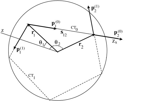
Figure 1: Trajectories connecting points ${\bf r}_{1}$ and ${\bf r}_{2}$ without (CT₀; solid line) and with reflections (CT₁; dashed line). Initial (${\bf p}_{1}^{(0)}$ and ${\bf p}_{1}^{(1)}$) and final momenta (${\bf p}_{2}^{(0)}$ and ${\bf p}_{2}^{(1)}$) of a particle at these points are also shown, together with the polar axises $z$ and $z_{s}$ and the corresponding angles $\theta_{1}$ and $\theta_{2}$.

Among all these CTs, one can find a short specific trajectory CT₀ without intermediate reflections from the nuclear boundary and other trajectories like CT₁ with reflections, as shown in Fig. 1 for the example of an infinitely deep spherical square-well potential. The first term in (II.1) can be approximated by the Green’s function of the locally free particle motion,

$$G_{{\rm CT}_{0}} \approx G_{0}=-\frac{m}{2\pi\hbar^{2}s}\;\hbox{exp}\left[\frac{ips}{\hbar}\right],$$

$$s=|{\bf s}|,\quad{\bf s} = {\bf r}_{2}-{\bf r}_{1},\quad p=\sqrt{2m\left[\varepsilon-V({\bf r})\right]},$$ (3)

with the modulus of the particle momentum $p$ in the mean-field potential $V({\bf r})$ ($p=\sqrt{2m\varepsilon}$ inside of a billiard potential). In (II.1), $S_{\rm CT}$ is the action for the motion of the particle along such a CT, and $\mu_{\rm CT}$ is the Maslov phase related to the catastrophe (turning and caustic) points along the CT strumag ; migdalrev ; MKApanSOL1 ; MAFptp2006 ; fed:jvmp ; masl ; fed:spm ; masl:fed . For the amplitude ${\cal A}_{\rm CT}$ in the semiclassical Green’s function (II.1) in the case of an unclosed isolated CT one has strumag ; sclbook ; gutz :

$$\!{\cal A}_{\rm CT}({\bf r}_{1},{\bf r}_{2};\varepsilon)\!=\!-\frac{1}{2\pi\hbar^{2}}\;|{\cal J}_{\rm CT}({\bf p}_{1},t_{\rm CT};{\bf r}_{2},\varepsilon)|^{1/2},$$ (4)

where ${\cal J}_{\rm CT}({\bf p}_{1},t_{\rm CT};{\bf r}_{2},\varepsilon)$ is the Jacobian for the transformation from the initial momentum ${\bf p}_{1}$ and time $t_{\rm CT}$ of the particle motion along the CT to its final coordinate ${\bf r}_{2}$ and energy $\varepsilon$. The specific expressions of the amplitudes ${\cal A}_{\rm CT}$ for the unclosed isolated trajectories (4) and one-parametric families of the degenerate closed periodic orbits in the infinitely deep spherical square-well potential were derived in strumag . For contributions of the one- and two-parametric degenerated families in the EGA amplitudes ${\cal A}_{\rm CT}$ for the case of the harmonic oscillator potential, one can refer to magosc .

The trace ${\bf r}_{2}\to{\bf r}_{1}$ of the first term $G_{{\rm CT}_{0}}({\bf r}_{1},{\bf r}_{2};\varepsilon)$ in (II.1) corresponds to the smooth level density of the ETF model, $g_{\rm ETF}(\varepsilon)$, sclbook ; bablo ; gutz ; strumag .

As well known strumag ; sclbook , other terms of the Green’s function in Eq. (II.1) are strongly oscillating components, due to $\hbar$ in the denominators of the exponents of (II.1). These oscillations become the stronger the smaller their period with increasing $S/\hbar$ in the imaginary exponent for the semiclassical asymptotic limit $\hbar\to 0$. The dimensionless parameter related to $\hbar$ is $\hbar/S_{\rm CT}$, which, for potentials with sharp walls, like billiards, is of the order of $\sim 1/k_{F}R\ll 1$ near the Fermi surface. Therefore, the convergence of the second term in Eq. (II.1) with respect to this semiclassical parameter appears only after averaging of the Green’s function traces (like level densities), over energies $\varepsilon$, or $kR$ for billiard-like potentials. Near the Fermi energy, this corresponds to an averaging over a large enough interval of the particle number $A$ through the radius $R$ [see Section IVA2, equation (89)]. The corresponding Strutinsky averaging strut ; fuhi ; sclbook ; magNPAE2010 ; migdalrev ; MKApanSOL1 ; MAFptp2006 with a Gaussian width $\widetilde{\Gamma}$, which covers at least a few major shells in the energy spectrum (see Appendix B3) leads to a local (${\bf r}_{2}\to{\bf r}_{1}$) smooth quantity, e.g., the level and particle density and the free energy of the statistical Thomas-Fermi model. The nonlocal (${\bf r}_{2}\neq{\bf r}_{1}$) contributions to the ETF transport coefficients become also important (Section IV). Therefore, we need a more extended statistical averaging in the phase space (energy and spatial coordinate) variables. This is similar to the averaging used in the derivation of the local hydrodynamical equations from the semiclassical kinetic equation within the many-body particle density or Green’s function formalism kadbaym ; kolmagpl .

II.2 PHASE-SPACE TRACE FORMULA

The level density, $g(\varepsilon)=\sum_{i}\delta(\varepsilon-\varepsilon_{i})$, determined by the energy spectrum $\varepsilon_{i}$ for the Hamiltonian $H({\bf r},{\bf p})$, can be obtained as a semiclassical approximation by using the phase-space trace formula in $\mathcal{D}$ dimensions ellipseptp ; spheroidpre ; spheroidptp ; MAFptp2006 :

$$g_{\rm scl}(\varepsilon) = \frac{1}{(2\pi\hbar)^{\mathcal{D}}}{\mbox{\rm Re}}\sum_{\rm CT}\int\hbox{d}{\bf r}^{\prime\prime}\int\hbox{d}{\bf p}^{\prime}$$ (5)

$$\times \delta\left(\varepsilon-H({\bf r}^{\prime\prime},{\bf p}^{\prime\prime})\right)\left|\mathcal{J}_{\rm CT}({\bf p}^{\prime}_{\perp},{\bf p}^{\prime\prime}_{\perp})\right|^{1/2}$$

$$\times \hbox{exp}\left\{\frac{i}{\hbar}\;\Phi_{\rm CT}-i\frac{\pi}{2}\mu_{\rm CT}\right\}\;,$$

where $\Phi_{\rm CT}$ is the phase integral related to the classical actions in suitable variables by

$$\Phi_{\rm CT} \equiv S_{\rm CT}({\bf p}^{\prime},{\bf p}^{\prime\prime};t_{\rm CT})-\left({\bf p}^{\prime}-{\bf p}^{\prime\prime}\right)\cdot{\bf r}^{\prime\prime}\!$$ (6)

$$= S_{\rm CT}({\bf r}^{\prime},{\bf r}^{\prime\prime};\varepsilon)+{\bf p}^{\prime}\cdot\left({\bf r}^{\prime}-{\bf r}^{\prime\prime}\right)\,$$

(see the derivations in MKApanSOL1 ). In (5), the sum is taken over all discrete CT manifolds for particle motion from the initial ${\bf r}^{\prime},{\bf p}^{\prime}$ to the final ${\bf r}^{\prime\prime},{\bf p}^{\prime\prime}$ point with a given energy $\varepsilon$ (see MAFptp2006 ). A CT can uniquely be specified by fixing, for instance, the initial condition ${\bf r}^{\prime\prime}$ and the final momentum ${\bf p}^{\prime}$ for a given time $t_{\rm CT}$ of the motion along the CT. $S_{\rm CT}({\bf p}^{\prime},{\bf p}^{\prime\prime};t_{\rm CT})$ is the action in the momentum representation,

$$S_{\rm CT}({\bf p}^{\prime},{\bf p}^{\prime\prime};t_{\rm CT})=-\int_{{\bf p}^{\prime}}^{{\bf p}^{\prime\prime}}\hbox{d}{\bf p}\cdot{\bf r}({\bf p})\;.$$ (7)

The integration by parts relates (7) to the action in the spatial coordinate space,

$$S_{\rm CT}({\bf r}^{\prime},{\bf r}^{\prime\prime};\varepsilon)=\int_{{\bf r}^{\prime}}^{{\bf r}^{\prime\prime}}\hbox{d}{\bf r}\cdot{\bf p}({\bf r})\;$$ (8)

(or other generating functions) by the Legendre transformation (6). The Maslov phase $\mu_{\rm CT}$ corresponds to the number of conjugate ( turning and caustics) points along the CT MAFptp2006 ; fed:jvmp ; masl ; fed:spm ). We introduced here a local phase-space 3D coordinate system, ${\bf r}=\{x,y,z\}$, $\,{\bf p}=\{p_{x},p_{y},p_{z}\}$, related to a PO which gives the main contribution into the trace integral among the CTs. The variables $x,p_{x}$ are locally the parallel and $\{{\bf r}_{\perp},{\bf p}_{\perp}\}$ the perpendicular ( with respect to a reference CT) phase-space coordinates (${\bf r}_{\perp}=\{y,z\}$, ${\bf p}_{\perp}=\{p_{y},p_{z}\}$ ) gutz ; smod ; sclbook . In (5), $\mathcal{J}_{\rm CT}({\bf p}^{\prime}_{\perp},{\bf p}^{\prime\prime}_{\perp})$ is the Jacobian for the transformation from the initial ${\bf p}_{\perp}^{\prime}$ to the final ${\bf p}_{\perp}^{\prime\prime}$ momentum, perpendicular to the CT.

For calculations of the trace integral by the SPM, one may write the stationary phase conditions in both ${\bf p}^{\prime}$ and ${\bf r}^{\prime\prime}$ variables. According to the definitions (6) and (7), the stationary phase condition for the ${\bf p}^{\prime}$ variable is the closing one in spatial coordinates:

$$\left(\frac{\partial\Phi_{\rm PO}}{\partial{\bf p}^{\prime}}\right)^{*}\equiv\left({\bf r}^{\prime}-{\bf r}^{\prime\prime}\right)^{*}=0\;.$$ (9)

Here and below a star on a quantity indicates that we evaluate that quantity at the stationary point, ${\bf p}^{\prime}={\bf p}^{\prime\;*}$. Thus, one has the closing condition, according to (9), $\Phi^{\ast}_{\rm PO}=S_{\rm PO}({\bf r}^{\prime},{\bf r}^{\prime\prime};\varepsilon)$. In the next integration over ${\bf r}^{\prime\prime}$ by the SPM we use the Legendre transformation (6). The stationary phase condition for this integration over the Cartesian spacial coordinates ${\bf r}={\bf r}^{\prime}={\bf r}^{\prime\prime}$ writes

$$\left(\frac{\partial\Phi_{\rm CT}}{\partial{\bf r}^{\prime}}\!+\!\frac{\partial\Phi_{\rm CT}}{\partial{\bf r}^{\prime\prime}}\right)^{*}\! \equiv \!\left(\frac{\partial S_{\rm CT}}{\partial{\bf r}^{\prime}}\!+\!\frac{\partial S_{\rm CT}}{\partial{\bf r}^{\prime\prime}}\right)^{*}\!$$ (10)

$$\equiv -\left({\bf p}^{\prime}-{\bf p}^{\prime\prime}\right)^{*}=0\;,$$

where the star means ${\bf r}^{\prime}={\bf r}^{\prime\prime}={\bf r}^{\ast}$ along with ${\bf p}^{\prime\;\ast}={\bf p}^{\prime\prime\ast}$, and one has the closing condition for a CT in the momentum space, too. Therefore, the stationary phase conditions are equivalent to the periodic-orbit equations (9) and (10). After applying these two conditions we arrive at the trace formula in terms of a sum over POs migdalrev ; sclbook .

II.3 THE TOTAL ISPM TRACE FORMULAS

The total ISPM trace formula is the sum of contributions of all POs (the isolated families with the classical degeneracy degree $\mathcal{K}\geq 1$ and the isolated orbits with ${\cal K}=0$),

$$\delta g_{\rm scl}(\varepsilon)=\sum_{\rm PO}\delta g_{\rm PO}(\varepsilon)$$ (11)

where

$$\delta g_{\rm PO}(\varepsilon)={\mbox{\rm Re}}\left\{{\cal B}_{\rm PO}\;\hbox{exp}\left[\frac{i}{\hbar}S_{\rm PO}(\varepsilon)-\frac{i\pi}{2}\mu_{\rm PO}\right]\right\},$$ (12)

with ${\cal B}_{\rm PO}$ the amplitude of the density oscillations depending on the PO classical degeneracy ${\cal K}$ and stability factors through the Green’s function amplitudes $\mathcal{A}_{\rm PO}$ gutz ; strumag . In (12), $S_{\rm PO}(\varepsilon)=\oint\hbox{d}{\bf r}\cdot{\bf p}$ is the action and $\mu_{\rm PO}$ the Maslov phase along the PO gutz ; strumag ; sclbook ; belyaev ; migdalrev ; MAFptp2006 . The Maslov phase $\mu_{\rm PO}$ is determined by the phase shifts through the turning and caustic points, according to the catastrophe Maslov&Fedoriuk theory fed:jvmp ; masl ; fed:spm ; masl:fed .

II.3.1 The averaged level density

.

For comparison with quantum densities we need also to average the trace formula (11) over the spectrum in a given mean-field potential. Since this trace formula has the simple form of a sum of separate PO terms everywhere including the bifurcations, one can take approximately analytically the integral over energies with the Gaussian weight factor (folding integral) strumag ; migdalrev ; MVApre2013 ; sclbook ; MAFptp2006 ; MKApanSOL1 . As a result for the averaged density $\delta g^{\rm scl}_{\Gamma}(\varepsilon)$, one obtains with this weight function for the averaging parameter $\Gamma$, which is much smaller than the Fermi energy $\varepsilon_{F}$,

$$\delta g^{\rm scl}_{\Gamma}(\varepsilon)\!=\!\sum_{\rm PO}\delta g_{\rm PO}(\varepsilon)\;\hbox{exp}\left[-\left(t_{\rm PO}\Gamma/\hbar\right)^{2}\right],$$ (13)

where $t_{\rm PO}=\partial S_{\rm PO}(\varepsilon)/\partial\varepsilon=Mt^{M=1}_{\rm PO}$ is the time period for a particle motion along the PO, accounting for the number of periods $M$, where $t^{(M=1)}_{\rm PO}$ is the period for a primitive (one cycle, $M=1$) PO.

The total ISPM level density as function of the energy $\varepsilon$ is given by

$$g^{\rm scl}_{\Gamma}(\varepsilon)=g_{ETF}(\varepsilon)+\delta g^{\rm scl}_{\Gamma}(\varepsilon)\;,$$ (14)

where $g_{\rm ETF}(\varepsilon)$ is the average part obtained within the ETF approximation sclbook . The convergence of the PO sum in (13) is provided mainly by the exponential Gaussian factor of this summand. Only the short-time POs (small-length POs for billiard potentials) give the main contributions to the PO sum (13) at a given finite averaging parameter $\Gamma$. According to (13), with increasing the PO period, $t_{\rm PO}$, and the averaging parameter, $\Gamma$, one finds a similar smearing out of the long-time PO contributions. For large $\Gamma$ (much larger than the distance $D$ between the neighbor s.p. levels but smaller or of order of the distance between the neighbor major shells, $D\ll\Gamma\hbox{\kern 1.00006pt\lower 2.58334pt\hbox{$\sim$} \kern-11.19997pt\raise 2.58334pt\hbox{$<$} \kern 1.00006pt}\hbar\Omega\ll\varepsilon_{F}$, where $\hbar\Omega\sim 2\pi/t_{\rm PO}\sim\varepsilon_{F}/A^{1/3}$), one finds the coarse-graining (major) shell-structure effects of short-time POs. For smaller $\Gamma$ ($D\hbox{\kern 1.00006pt\lower 2.58334pt\hbox{$\sim$} \kern-11.19997pt\raise 2.58334pt\hbox{$<$} \kern 1.00006pt}\Gamma\ll\hbar\Omega$), one observes a fine-reserved shell structure involving the long-time POs. In this case, the amplitudes $\mathcal{B}_{\rm PO}$ can be enhanced by the bifurcation phenomena smod ; spheroidptp ; MAFptp2006 ; MVApre2013 ; MKApanSOL1 .

II.3.2 Energy shell corrections

The PO expansion for the energy shell corrections $\delta E_{\rm scl}$ writes strumag ; ellipseptp ; spheroidptp ; MVApre2013 ; sclbook ; migdalrev ; belyaev ; MKApanSOL1

$$\delta E=d_{s}\sum_{\rm PO}\frac{\hbar^{2}}{t_{\rm PO}^{2}}\,\delta g_{\rm PO}(\varepsilon_{F})\;,$$ (15)

where $t_{\rm PO}=Mt^{M=1}_{\rm PO}(\varepsilon_{F})$ is the time of particle motion along the PO (taking into account its repetition number $M$) at the Fermi energy $\varepsilon=\varepsilon_{F}$, where $t^{M=1}_{\rm PO}$ is the time of particle motion along the primitive ($M=1$) PO (at $\varepsilon=\varepsilon_{F}$). The factor $d_{s}$ takes into account the spin (spin-isospin) degeneracy for neutron and/or proton Fermi systems. The Fermi energy $\varepsilon_{F}$ is related to the conservation of the particle number $A$ through the equation:

$$A=d_{s}\int_{0}^{\varepsilon_{F}}\hbox{d}\varepsilon\,g(\varepsilon)\;.$$ (16)

Note that the energy shell corrections $\delta E$ which are the observed physical quantities do not contain arbitrary averaging parameter $\Gamma$, in contrast to the level density $g^{\rm scl}_{\Gamma}(\varepsilon)$ (14). The convergence of the PO sum (15) is ensured by the additional factor in front of the density component $\delta g_{\rm PO}$ which is inversely proportional to the time $t_{\rm PO}$ squared along the PO. Therefore, we need short-time POs if they occupy enough large phase-space volumes.

Within the POT, at a given temperature $T$, after the statistical averaging over the canonical ensemble, one obtains the PO sum for the semiclassical free-energy shell correction $\delta{\cal F}_{\rm scl}$ strumag ; kolmagstr ; fraukolmagsan ; mskbPRC2010 ; belyaev :

$$\delta\mathcal{F}=\sum_{\rm PO}\frac{\pi t_{\rm PO}T/\hbar}{\hbox{sinh}(\pi t_{\rm PO}T/\hbar)}\;\delta E_{\rm PO}\;,$$ (17)

where $\delta E_{\rm PO}$ is the PO component of the energy shell correction,

$$\delta E_{\rm PO}=d_{s}\,\frac{\hbar^{2}}{t_{\rm PO}^{2}}\;\delta g_{\rm PO}(\lambda)\;,$$ (18)

and $\delta g_{\rm PO}(\lambda)$ is the PO component (12) in the oscillating level density (11) at the chemical potential $\varepsilon=\lambda$. The oscillating (free) energy shell correction, $\delta\mathcal{F}$ (17), is function of the particle number, $A$, through the chemical potential $\lambda$, which, at small temperatures $T$, equals approximately the Fermi energy $\varepsilon_{F}$, [$\lambda\approx\varepsilon_{F}$, see (16)]. Notice that, in addition to the $1/t^{2}_{\rm PO}$ factor of the PO energy shell-correction component (15), there is the temperature-dependent factor, which leads to the exponential decrease of the contributions of long-time POs, and ensures the convergence of the PO sum in the free-energy shell correction (17). The temperature $T$ in (17) for $\delta\mathcal{F}$ takes a similar role concerning the convergence of the PO sum as the averaging parameter $\Gamma$ in the averaged level-density shell correction (13). With increasing temperature $T$, one finds the exponential decrease of the oscillating free-energy shell correction, i.e., an exponential disappearance of the shell effects in the free energy. For finite temperature, one obtains such a disappearance of the long-time POs, such that only the short-time POs give the main contributions to the PO sum (17). The critical temperature $T_{\rm cr}\approx\pi/\hbar\Omega\approx 2-3$ MeV for the disappearance of the shell effects in heavy nuclei ($A=100-200$) (see, e.g., strumag ; mskbPRC2010 ; belyaev ; kolmagstr ) is in good agreement with the quantum SCM calculations fuhi . See more specific expressions of $\delta g_{\rm PO}$ (12) in terms of the PO classical degeneracy, the stability factors, and the action along the PO in gutz ; strumag ; sclbook ; belyaev ; migdalrev ; MKApanSOL1 . The POs appear through the stationary phase conditions (9) and (10) (which, in the present context, is equivalent to the PO condition MAFptp2006 ) for the calculation of integrals over ${\bf r}^{\prime\prime}$ and ${\bf p}^{\prime}$ in (5) by the ISPM spheroidptp ; MAFptp2006 ; migdalrev ; MKApanSOL1 .

II.4 SPHERICAL ACTION-ANGLE VARIABLES

We now transform the phase space trace formula (5) from the Cartesian phase space variables $\{{\bf r},{\bf p}\}$ to the canonical angle-action ones $\{{\bf\Theta},{\bf I}\}$. The latter variables have a clearer physical meaning, and are simpler to use for integrable Hamiltonians. For integrable systems, the action-angle variables are particularly useful because the Hamiltonian $H$ does not depend on the angle variables ${\bf\Theta}$, i.e., $H=H({\bf I})$. Since the angles ${\bf\Theta}$ are the cyclic variables in this integrable case, the corresponding action variables ${\bf I}$ are the integrals of the particle motion. Therefore, from (5) one has

$$g_{\rm scl}(\varepsilon) = \frac{1}{(2\pi\hbar)^{3}}{\mbox{\rm Re}}\sum_{\rm CT}\int\hbox{d}{\bf\Theta}^{\prime\prime}\,\int\hbox{d}{\bf I}\,$$ (19)

$$\times \delta(\varepsilon-H({\bf I}))\left|\mathcal{J}_{\rm CT}({\bf p}^{\prime\prime}_{\perp},{\bf p}^{\prime}_{\perp})\right|^{1/2}\times$$

$$\times \hbox{exp}\left[\frac{i}{\hbar}\Phi_{\rm CT}-\frac{i\pi}{2}\mu_{\rm CT}\right]\;.$$

The phase integral $\Phi_{\rm CT}$ (6), as expressed in terms of the action-angle variables through the actions (7) or (8) (standard generating functions) are considered, in the mixed representation. The Jacobian ${\cal J}({\bf p}^{\prime\prime}_{\perp},{\bf p}^{\prime}_{\perp})$ is also transformed to the new variables. We took also into account explicitly that the actions ${\bf I}$ are constants of motion for a spherical integrable Hamiltonian, omitting the upper subscripts in ${\bf I}$ as related to their initial (prime) and final (double prime) values. We used also usual Jacobian determinant transformations from a set of variables to another set, taking into account that there is no variations in a parallel x direction along the PO, and the Jacobian of the canonical transformations equals one. Note that in spite of the non-orthogonality of the angle-action coordinate system there are still the definite relations between the parallel (or perpendicular) components of the quantities expressed in terms of the action $S_{\rm CT}({\bf r}^{\prime},{\bf r}^{\prime\prime};\varepsilon)$ in the Cartesian and in the angle-action coordinate system, because of the conservation of the actions $I_{i}$ for integrable Hamiltonians along a trajectory CT MAFptp2006 . Therefore, it makes sense to relate the $x$ components $I_{x}$ and $\Theta_{x}$ and the corresponding $y,z$ components of actions and the corresponding angles to the “parallel” and “perpendicular” components with respect to the reference PO in the final trace formula (19), respectively.

PO solutions to the stationary phase equations (9) and (10) are also invariants with respect to the considered canonical transformation as Hamiltonian, altogether that always can be expressed through both the Cartesian, and the angle-action coordinate system by using the suitable transformation equations.

III THE ETF EFFECTIVE SURFACE APPROACH

The explicit and accurate analytical expressions for the particle density distributions were obtained within the nuclear ES approximation strtyap ; strmagbr ; strmagden . They take advantage of the saturation properties of nuclear matter in the narrow diffuse-edge region in finite heavy nuclei. The ES is defined as the location of points with a maximal density gradient. An orthogonal coordinate system related locally to the ES is specified by the distance $\xi$ of a given point from the ES and a tangent coordinate parallel to the ES. Using the nuclear energy-density functional theory rungegrossPRL1984 ; marquesgrossARPC2004 , one can simplify the variational condition derived from minimization of the nuclear energy at some fixed integrals of motion in these coordinates within the leptodermous approximation. In particular, in the ETF approach brguehak , this can be done in sufficiently heavy nuclei for any fixed deformation using the expansion in a small parameter $a/R\sim A^{-1/3}\ll 1$, where $a$ is of the order of the diffuse edge thickness of the nucleus, $R$ is the mean-curvature radius of the ES, and $A$ the number of nucleons. The accuracy of the ES approximation in the ETF approach was checked strmagden without the spin-orbit (SO) and asymmetry terms by comparing the results with those of Hartree-Fock (HF) and other ETF models for some Skyrme forces. The ES approach strmagden was also extended by taking into account the SO and asymmetry effects magsangzh ; BMVnpae2012 ; BMRV ; BMRPhysScr2014 .

Solutions for the isoscalar and isovector particle densities and energies in the ES approximation of the ETF approach were applied to analytical calculations of the surface symmetry energy, the neutron skin and isovector stiffness coefficient in the leading order of the parameter $a/R$ BMRV . Our results are compared with older investigations myswann69 ; myswnp80pr96 ; myswprc77 ; myswiat85 within the LDM and with more recent works vretenar1 ; vretenar2 ; ponomarev ; danielewicz1 ; pearson ; danielewicz2 ; vinas1 ; vinas2 ; vinas4 ; vretenar3 ; kievPygmy ; nester1 ; nester2 ; nester3 ; vinas5 .

The splitting of the IVDR into the main and satellite peaks kievPygmy ; nester1 ; nester2 ; BMRPhysScr2014 ; BMRps2015 ; BMRprc2015 ; endres was obtained as function of the isovector surface-energy constant within the FLDM kolmag ; kolmagsh in the ES approach. The analytical expressions for the surface symmetry-energy constants have been tested by the IVDR energies and sum rules within the FLDM BMRPhysScr2014 ; BMRps2015 ; BMRprc2015 for some Skyrme forces neglecting derivatives of the nongradient terms in the symmetry energy density per particle with respect to the mean particle density. In the present review, following BMRprc2015 , we shall extend the variational-ES method accounting for these derivatives introduced originally by Swiatecki and Myers within the LDM myswann69 .

In Section IIIA, we give an outlook of the basic points of the ES approximation within the density-functional theory. The main results for the isoscalar and isovector particle densities are presented in Section IIIB with emphasizing the derivatives of the symmetry energy density per particle. Section IIIC is devoted to analytical derivations of the symmetry energy in terms of the surface energy coefficient, the neutron skin thickness and the isovector stiffness including these derivatives. Sections IIID and IIIV are devoted to the collective dynamical description of the IVDR structure in terms of the response functions and transition densities. Discussions of the results are given in Section IIIVI and summarized at the end of this section. Some details of calculations are presented in Appendix A.

III.1 SYMMETRY ENERGY AND PARTICLE DENSITIES

We start with the nuclear energy $E$ as a functional of the isoscalar ($\rho_{+}$) and isovector ($\rho_{-}$) densities $\rho_{\pm}=\rho_{n}\pm\rho_{p}$ in the local density approach brguehak ; chaban ; reinhard ; bender ; revstonerein ; reinhardSV ; ehnazarrrein ; pastore ; jmeyer :

$$E=\int\hbox{d}{\bf r}\;\rho_{+}\mathcal{E}\left(\rho_{+},\rho_{-}\right),$$ (20)

where $\mathcal{E}\left(\rho_{+},\rho_{-}\right)$ is the energy density per particle,

$$\mathcal{E}\!\left(\rho_{+},\rho_{-}\!\right)\!=\!-\!b_{\rm V}\!+\!JI^{2}\!+\!\varepsilon_{+}(\rho_{+})\!+\!\varepsilon_{-}(\rho_{+},\rho_{-}\!)\!$$ (21)

$$+\left(\frac{\mathcal{C}_{+}}{\rho_{+}}+{\cal D}_{+}+\frac{\Gamma}{4\rho_{+}^{2}}\right)\left(\nabla\rho_{+}\right)^{2}$$

$$+ \left(\frac{\mathcal{C}_{-}}{\rho_{+}}+{\cal D}_{-}\right)\left(\nabla\rho_{-}\right)^{2}.$$

Here, $b_{\rm V}\approx$ 16 MeV is the separation energy of a particle, $J\approx$ 30 MeV is the main volume symmetry-energy constant of infinite nuclear matter, and $~{}I=(N-Z)/A$ the asymmetry parameter; $~{}N=\int\hbox{d}{\bf r}\rho_{n}({\bf r})$ and $~{}Z=\int\hbox{d}{\bf r}\rho_{p}({\bf r})$ are the neutron and proton numbers, and $~{}A=N+Z$. These constants determine the first two terms of the volume energy. The last four terms are surface terms: The first two terms are independent of the gradients of the particle densities, and the last two ones depend on these gradients. For the first surface term independent of the gradients, $\varepsilon_{+}$, one can simply use

$$\varepsilon_{+}(\rho_{+})=\frac{K_{+}}{18}\;e_{+}\left[\epsilon(w_{+})\right],$$ (22)

where $K_{+}\approx 220-245$ MeV (see Table 1) is the isoscalar in-compressibility modulus of symmetric nuclear matter, $w_{+}$ is the dimensionless isoscalar-particle density, $w_{+}=\rho_{+}/\overline{\rho}$, and

$$e_{+}\left[\epsilon\left(w_{+}\right)\right]=9\epsilon^{2}+I^{2}\left[\mathcal{S}_{\rm sym}(\epsilon)-J\right]/K_{+}\;.$$ (23)

The small parameter $\epsilon$,

$$\epsilon=\frac{\overline{\rho}-\rho_{+}}{3\overline{\rho}}=\frac{1-w_{+}}{3}\;,$$ (24)

is used in the expansion,

$$\mathcal{S}_{\rm sym}(\epsilon)=J-L\epsilon+\frac{K_{-}}{2}\epsilon^{2}+\cdots\;,$$ (25)

around the particle density of infinite nuclear matter $\overline{\rho}=3/4\pi r_{0}^{3}\approx$ 0.16 fm^-3, and $r_{0}$ is the commonly accepted constant in the $A^{1/3}$ dependence of a mean radius. Several other constants, $L$ and $K_{-}$, which were introduced by Myers and Swiatecki myswann69 , will be explained below. The next isovector surface term $\varepsilon_{-}(\rho_{+},\rho_{-})$ in (21) can be defined through the same function $\mathcal{S}_{\rm sym}(\epsilon)$ (25):

$$\varepsilon_{-}\left(\rho_{+},\rho_{-}\right)=\mathcal{S}_{\rm sym}(\epsilon)\;\left(\frac{\rho_{-}}{\rho_{+}}\right)^{2}-JI^{2}.$$ (26)

For the first and second derivatives of $\mathcal{S}_{\rm sym}(\epsilon)$ with respect to $\epsilon$, one can take in (25) the derivative values $L\approx 20\div 120$ MeV and, even less known, $K_{-}$ PR2008 ; vinas1 ; vinas5 . The constants $\mathcal{C}_{\pm}$ and $\mathcal{D}_{\pm}$ in (21) are defined by the parameters of the Skyrme forces brguehak ; bender ; chaban ; reinhardSV ; pastore ,

$$\mathcal{C}_{+} = \frac{1}{12}\left(t_{1}-\frac{25}{12}t_{2}-\frac{5}{3}t_{2}x_{2}\right),$$

$$\mathcal{C}_{-} = -\frac{t_{1}}{48}\left(1+\frac{5}{2}x_{1}\right)-\frac{t_{2}}{36}\left(1+\frac{19}{8}x_{2}\right).$$ (27)

The isoscalar SO gradient terms in (21) are defined with a constant: $\mathcal{D}_{+}=-9mW_{0}^{2}/16\hbar^{2}$, where $W_{0}\approx$ 100 - 130 MeV$\cdot$fm⁵ and $m$ is the nucleon mass. The constant $\mathcal{D}_{-}$ is usually relatively small and will be neglected below for simplicity. Within the ETF, the terms proportional to $\Gamma$ of the gradient part in (21) is coming from the $\hbar^{2}$ correction to the TF kinetic energy density sclbook , $\Gamma=\hbar^{2}/18m$ (Appendix D). Equation (21) can be applied in a semiclassical approximation for a realistic Skyrme force chaban ; reinhard ; bender ; revstonerein ; ehnazarrrein , in particular by neglecting higher $\hbar$ corrections in the ETF kinetic energy brguehak ; strmagbr ; strmagden and also Coulomb terms. All of them can be easily taken into account strtyap ; strmagden ; magsangzh neglecting relatively small Coulomb exchange terms. Such exchange terms can be calculated numerically in extended Slater approximations GU-HQ2013_PRC87-041301 .

The energy density per particle in (21) contains the first two volume terms, and the surface components including the new $L$ and $K_{-}$ derivative corrections of $\varepsilon_{-}$ (26), along with the isoscalar and isovector density-gradient terms. Both are important for finite nuclear systems. These gradient terms, together with the other surface components in the energy density (21), within the ES approximation are responsible for the surface tension in finite nuclei.

As usual, we minimize the energy $E$ under the constraints of fixed particle number $A=\int\hbox{d}{\bf r}\;\rho_{+}({\bf r})$ and neutron excess $N-Z=\int\hbox{d}{\bf r}\;\rho_{-}({\bf r})$ using the Lagrange multipliers $\lambda_{+}$ and $\lambda_{-}$ with the isoscalar and isovector chemical-potential surface corrections (see Appendix A). Taking also into account additional deformation constraints (like the quadrupole moment), our approach can be applied for any deformation parameter of the nuclear surface, if its diffuseness $a$ is small with respect to the curvature radius $R$. Approximate analytical expressions of the binding energy will be obtained at least up to order $A^{2/3}$. To satisfy the condition of particle number conservation with the required accuracy we account for relatively small surface corrections ($\propto a/R\sim A^{-1/3}$ in first order) to the leading terms in the Lagrange multipliers strmagbr ; strmagden ; magsangzh ; BMRV . We take into account explicitly the diffuseness of the particle density distributions. Solutions of the variational Lagrange equations can be derived analytically for the isoscalar and isovector surface-tension coefficients (surface energy constants), instead of the phenomenological constants of the standard LDM myswann69 (the neutron and proton particle densities were considered earlier to be distributions with a strictly sharp edge while, in the ES approach, the ES is diffused).

III.2 ISOSCALAR AND ISOVECTOR DENSITIES

For the isoscalar particle density, $w=\rho_{+}/\overline{\rho}$, one has up to leading terms in the leptodermous parameter $a/R$ the usual first-order differential Lagrange equation strmagden ; magsangzh ; BMRV ; BMRps2015 ; BMRprc2015 . Integrating this equation, one finds the solution:

$$x=-\int\limits_{w_{r}}^{w}\hbox{d}y\;\sqrt{\frac{1+\beta y}{y\;e_{+}[\epsilon(y)]}}\;,\qquad x=\frac{\xi}{a}\;,$$ (28)

for $x<x(w=0)$ and $w=0$ for $x\geq x(w=0)$, where $x(w=0)$ is the turning point. $\beta=\mathcal{D}_{+}\overline{\rho}/\mathcal{C}_{+}$ is the dimensionless SO parameter, see (23) for $e_{+}[\epsilon(y)]$ (for convenience, we often omit the lower index “$+$” in $w_{+}$ ). For $w_{r}=w(x=0)$, one has the boundary condition, $\hbox{d}^{2}w(x)/\hbox{d}x^{2}=0$ at the ES ($x=0$):

$$e_{+}\![\epsilon(w_{r})]\!+\!w_{r}(1\!+\!\beta w_{r})\left[\frac{\hbox{d}e_{+}[\epsilon(w)]}{\hbox{d}w}\right]_{w=w_{r}}\!=\!0\;.$$ (29)

In (28), $a\approx 0.5-0.6$ fm is the diffuseness (mean-squared) parameter strmagden ; magsangzh ; BMRV ,

$$a=\sqrt{\frac{\mathcal{C}_{+}\overline{\rho}K_{+}}{30b_{V}^{2}}},$$ (30)

found from the asymptotic behavior of the particle density, $w\sim\hbox{exp}(-\xi/a)$ for large $\xi$ ($\xi\gg a$).

As shown in strmagden ; magsangzh , the influence of the semiclassical $\hbar$ corrections (related to the ETF kinetic energy) to $w(x)$ is negligibly small everywhere, except for the quantum tail outside the nucleus ($x\hbox{\kern 1.00006pt\lower 2.58334pt\hbox{$\sim$} \kern-11.19997pt\raise 2.58334pt\hbox{$>$} \kern 1.00006pt}1$). Therefore, all these corrections were neglected in (21). With a good convergence of the expansion of $e_{+}[\epsilon(y)]$ in powers of $1-y$ up to the quadratic term strmagden ; magsangzh and small $I^{2}$ corrections in (23), $e=(1-y)^{2}$, one explicitly finds analytical solutions of (28) in terms of the algebraic, trigonometric and logarithmic functions BMRV . For $\beta=0$ (i.e. , without SO terms), it simplifies to the solution $w(x)=\tanh^{2}\left[(x-x_{0})/2\right]$ for $x<x_{0}=2{\rm arctanh}(1/\sqrt{3})$ and zero for $x$ outside the nucleus ($x\geq x_{0}$). As shown in Appendix A1, for $\mathcal{C}_{\pm}=\mathcal{D}_{\pm}=0$, one obtains the well-know solution $w(x)=1/[1+\hbox{exp}(x)]$, symmetrical with respect to the ES, in contrast to the results mentioned above for a finite $\beta$.

After simple transformations of the isovector Lagrange equation (A.1), one similarly finds up to the leading term in $a/R$ in the ES approximation for the isovector density, $w_{-}(x)=\rho_{-}/(\overline{\rho}I)$, the equation and the boundary condition (A1). The analytical solution $w_{-}=w\hbox{cos}[\psi(w)]$ can be obtained through the expansion (A.5) of $\psi$ in powers of

$$\gamma(w)=\frac{3\epsilon}{c_{\rm sym}},\qquad c_{\rm sym}=a\;\sqrt{\frac{J}{\overline{\rho}\;|\mathcal{C}_{-}|}}\;.$$ (31)

Expanding up to the second order in $\gamma$, one obtains (Appendix A1)

$$w_{-}=w\;\hbox{cos}\left[\psi(w)\right]\approx w\left(1-\frac{\psi^{2}(w)}{2}\!+\!\cdots\!\right),$$ (32)

with

$$\psi(w)=\frac{\gamma(w)}{\sqrt{1+\beta}}\;\left[1+\widetilde{c}\gamma(w)+\cdots\right],$$ (33)

$$\widetilde{c}=\frac{\beta c_{\rm sym}^{2}+2+c_{\rm sym}^{2}L(1+\beta)/(3J)}{2c_{\rm sym}(1+\beta)};$$ (34)

see also the constant $c_{3}$ at higher (third) order corrections. Notice that $w_{-}$ depends on $L$ in second order in $\gamma$ but it is independent of $K_{-}$ at this order.

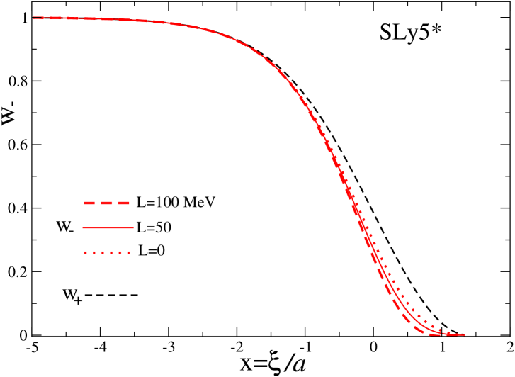
Figure 2: Dimensionless isoscalar and isovector particle densities, $w_{+}$ and $w_{-}$ respectively, as function of the (dimensionless) distance to the ES $x=\xi/a$ for the SLy5 Skyrme interaction (thin dashed and solid lines, respectively). To investigate the sensitivity with respect to variations of $L$, the isovector density is displayed for three different values of the droplet model parameter $L$, keeping all other parameters unchanged.

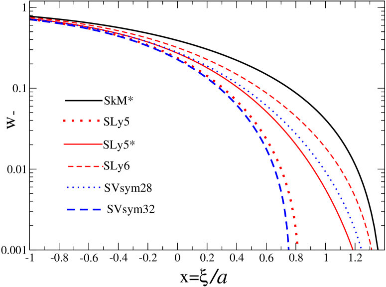
Figure 3: Dimensionless isovector density $w_{-}$ (on a logarithmic scale) as function of the (dimensionless) distance to the ES $x=\xi/a$ obtained for several Skyrme forces within the quadratic approximation to e+[(w)].

In Fig. 2, the $L$ dependence of the function $w_{-}(x)$ is shown within approximately the total interval from $L=0$ to $L=100$ MeV vinas2 , and it is compared to that of the density $w(x)$ for the SLy5* force as a typical example. As shown in Fig. 3 in a larger (logarithmic) scale, one observes notable differences in the isovector densities $w_{-}$ derived from different Skyrme forces chaban ; reinhardSV within the edge diffuseness. All these calculations have been done with the finite proper value of the slope parameter $L$. For SLy forces this value is taken from jmeyer , for $SGII$ from vinas2 and for others from reinhardSV (Table 1). As shown below, this is in particular important for calculations of the neutron skin of nuclei. Notice that, with the precision of line thickness, our results are almost the same taking approximately $L=50$ MeV for SLy5* and $L=60$ MeV for SVsym32. Note also that, up to second order in the small parameter $\gamma$, the isovector particle density $w_{-}$ in (32) does not depend on the symmetry energy in-compressibility $K_{-}$. The $K_{-}$ dependence appears only at higher (third) order terms in the expansion in $\gamma$ (Appendix A1). Therefore, as a first step of the iteration procedure, it is possible to study first the main slope effects of $L$ neglecting small $I^{2}$ corrections to the isoscalar particle density $w_{+}$ (28) through $e_{+}$ (23). Then, we may study more precisely the effect of the second derivatives $K_{-}$ taking into account higher order terms.

We emphasize that the dimensionless densities, $w(x)$ (see (28) and BMRV ; BMRps2015 ) and $w_{-}(x)$ (32), shown in Figs. 2 and 3, were obtained in the leading ES approximation ($a/R\ll 1$) as functions of specific combinations of Skyrme force parameters as $\beta$ and $c_{\rm sym}$ (31) accounting for the $L$-dependence (34). These densities are at leading order in the leptodermous parameter $a/R$ approximately universal functions, independent of the properties of specific nucleus. It yields largely the local density distributions in the normal-to-ES direction $\xi$ with the correct asymptotic behavior outside of the deformed ES layer at $a/R\ll 1$, as it is the case for semi-infinite nuclear matter. Therefore, at the dominating order, the particle densities $w_{\pm}$ are universal distributions independent of the specific properties of the nucleus while higher order corrections to the densities $w_{\pm}$ depend, indeed, on its specific macroscopic properties.

III.3 ISOVECTOR ENERGY AND STIFFNESS

The nuclear energy $E$ [equation (20)] in the improved ES approximation (Appendix A3) is split into the volume and surface terms BMRV ; BMRprc2015 ,

$$E\approx-b_{\rm V}\;A+J(N-Z)^{2}/A+E_{\rm S}\;.$$ (35)

For the surface energy $E_{\rm S}$ one obtains

$$E_{\rm S}=E_{\rm S}^{(+)}+E_{\rm S}^{(-)}$$ (36)

with the isoscalar (+) and isovector (-) surface components:

$$E_{\rm S}^{(\pm)}=b_{\rm S}^{(\pm)}\frac{\mathcal{S}}{4\pi r_{0}^{2}}\;,$$ (37)

where $\mathcal{S}$ is the surface area of the ES, $b_{\rm S}^{(\pm)}$ are the isoscalar $(+)$ and isovector $(-)$ surface-energy constants,

$$b_{\rm S}^{(\pm)}\approx 8\pi r_{0}^{2}\mathcal{C}_{\pm}\!\int_{-\infty}^{\infty}\!\hbox{d}\xi\!\left(1+\frac{\mathcal{D}_{\pm}}{\mathcal{C}_{\pm}}\rho_{+}\right)\left(\frac{\partial\rho_{\pm}}{\partial\xi}\right)^{2}.$$ (38)

These constants are proportional to the corresponding surface tension coefficients $\sigma_{\pm}=b_{\rm S}^{(\pm)}/(4\pi r_{0}^{2})$ through the solutions (28) and (32) for $\rho_{\pm}(\xi)$, which can be taken into account in leading order of $a/R$ (Appendix A) . These coefficients $\sigma_{\pm}$ are the same as found in the expressions for capillary pressures of the macroscopic boundary conditions; see Appendix A2, and strmagbr ; strmagden ; magsangzh ; BMRV with new values $\varepsilon_{\pm}$ modified by $L$ and $K_{-}$ derivative corrections of (23) and (26), also BMRps2015 ; BMRprc2015 ). Within the improved ES approximation where higher order corrections in the small parameter $a/R$ are taken into account, we derived in BMRV equations for the nuclear surface itself (see also strmagbr ; strmagden ; magsangzh ). For more exact isoscalar and isovector particle densities we account for the main terms at next order of the parameter $a/R$ in the Lagrange equations [see (A.1) for the isovector and strmagbr ; strmagden ; magsangzh for the isoscalar case]. Multiplying these equations by the corresponding $\partial\rho_{\pm}/\partial\xi$ and integrating them over the ES in the normal-to-surface direction $\xi$ and using the solutions for $w_{\pm}(x)$ up to the leading orders [(28) and (32)], one arrives at the ES equations in the form of the macroscopic boundary conditions (Appendix A2 and strmagbr ; strmagden ; magsangzh ; kolmagsh ; magstr ; magboundcond ; bormot ; BMRV . They ensure equilibrium through the equivalence of the volume and surface (capillary) pressure variations. As shown in Appendix A2, the latter ones are proportional to the corresponding surface tension coefficients $\sigma_{\pm}$.

For the energy surface coefficients $b_{\rm S}^{(\pm)}$ (38), one obtains

$$b_{\rm S}^{(+)} = 6\mathcal{C}_{+}\overline{\rho}\mathcal{J}_{+}/(r_{0}a),$$

$$\mathcal{J}_{+} = \int\limits_{0}^{1}\hbox{d}w\sqrt{w(1+\beta w)\;e_{+}[\epsilon(w)]},$$ (39)

$$b_{\rm S}^{(-)}=k_{S}\;I^{2},\qquad k_{\rm S}=6\overline{\rho}\;\mathcal{C}_{-}\;\mathcal{J}_{-}/(r_{0}a),$$ (40)

$$\mathcal{J}_{-}=\int\limits_{0}^{1}\hbox{d}w\;\sqrt{\frac{w\;e_{+}[\epsilon(w)]}{1+\beta w}}\left\{\hbox{cos}(\psi)\;\right.$$ (41)

$$+ \left.\frac{w\hbox{sin}(\psi)}{c_{\rm sym}\sqrt{1+\beta}}\left[1+2\widetilde{c}\gamma(w)\right]\right\}^{2}\approx\int_{0}^{1}\hbox{d}w(1-w)$$

$$\times \sqrt{\frac{w}{1+\beta w}}\;\left\{1+\frac{2\gamma(w)}{c_{\rm sym}(1+\beta)}+\left(\frac{\gamma}{1+\beta}\right)^{2}\right.$$

$$\times \left.\left[\frac{1}{c_{\rm sym}^{2}}+6(1+\beta)\left(\frac{\widetilde{c}}{c_{\rm sym}}-\frac{1}{2}\right)\right]\right\},$$

see (31) and (34) for $\gamma$ and $\widetilde{c}$, respectively. Simple expressions for the constants $b_{\rm S}^{(\pm)}$ in (III.3) and (40) can be easily derived explicitly in terms of algebraic and trigonometric functions by calculating analytically integrals over $w$ for the quadratic form of $e_{+}[\epsilon(w)]$ [(A.16) and (A.18)]. Note that in these derivations, we neglected curvature terms and, being of the same order, shell corrections, which have been discarded from the very beginning of Section III. The isovector energy-density terms were obtained within the ES approximation with high accuracy up to the product of two small quantities, $I^{2}$ and $(a/R)^{2}$.

According to the macroscopic theory myswann69 ; myswnp80pr96 ; myswprc77 ; BMRV ; BMRprc2015 , one may define the isovector stiffness $Q$ with respect to the difference $R_{n}-R_{p}$ between the neutron and proton radii as a dimensionless collective variable $\tau$,

$$E_{\rm S}^{(-)} = -\frac{\overline{\rho}r_{0}}{3}\oint\hbox{d}S\;Q\tau^{2}\approx-\frac{Q\tau^{2}\mathcal{S}}{4\pi r_{0}^{2}}\;,$$

$$\tau = \left(R_{n}-R_{p}\right)/r_{0}\;,$$ (42)

where $\tau$ is the relative neutron skin. Comparing this expression to equation (37) for the isovector surface energy written through the isovector surface-energy constant $b_{\rm S}^{(-)}$ (40), one obtains

$$Q=-k_{\rm S}\frac{I^{2}}{\tau^{2}}\;.$$ (43)

Defining the neutron and proton radii $R_{n,p}$ as positions of maxima of the neutron and proton density gradients, respectively, one finds the neutron skin $\tau$ BMRV ; BMRprc2015 ,

$$\tau=\frac{8aI}{r_{0}c_{\rm sym}^{2}}\varsigma(w_{r}),$$ (44)

where

$$\varsigma(w)\! = \!\frac{w^{3/2}(1+\beta w)^{5/2}}{(1\!+\!\beta)(3w\!+\!1\!+\!4\beta w)}\left\{w(1+2\widetilde{c}\gamma)^{2}\!\right.$$ (45)

$$+ \left.2\gamma\left(1+\widetilde{c}\gamma\right)\left[\widetilde{c}w-c_{\rm sym}\left(1+2\widetilde{c}\gamma\right)\right]\right\}$$

is taken at the ES value $w_{r}$ (29). Finally, taking into account equations (43) and (40), one arrives at

$$Q=-\nu\;\frac{J^{2}}{k_{\rm S}},\qquad\nu=\frac{k_{\rm S}^{2}I^{2}}{\tau^{2}J^{2}}=\frac{9\mathcal{J}_{-}^{2}}{16\varsigma^{2}(w_{r})}\;,$$ (46)

where $\mathcal{J}_{-}$ and $\varsigma(w)$ are given by (41) and (45), respectively. Note that $Q=-9J^{2}/4k_{\rm S}$ has been predicted in myswann69 ; myswnp80pr96 : For $\nu=9/4$, the first part of (46), which relates $Q$ with the volume symmetry energy $J$, and the isovector surface-energy constant $k_{\rm S}$, is identical to that used in myswann69 ; myswnp80pr96 ; myswprc77 ; myswiat85 ; vinas1 ; vinas2 . However, in our derivations $\nu$ deviates from $9/4$, and it is proportional to the function $\mathcal{J}_{-}^{2}/\varsigma^{2}(w_{r})$. This function depends significantly on the SO interaction parameter while $\beta$ is approximately insensitive on the specific Skyrme force BMRV .

The approximate universal functions $w(x)$, ((28) and BMRV ), and $w_{-}(x)$ (32) can be used in the leading order of the ES approximation for calculations of the surface energy coefficients $b_{S}^{(\pm)}$ (38), and the neutron skin $\tau\propto I$ (44). As shown in BMRV and in Appendix A3, here only the particle density distributions $w(x)$ and $w_{-}(x)$ are needed within the surface layer through their derivatives. The lower limit of the integration over $\xi$ in (38) can be then approximately extended to $-\infty$ because there are no contributions from the internal volume region in evaluations of the main surface terms of the pressure and energy. Therefore, the surface symmetry-energy coefficient $k_{S}$ in (40) and (A.18) , the neutron skin $\tau$ (44), and the isovector stiffness $Q$ (46) can be approximated analytically in terms of functions of definite critical combinations of the Skyrme parameters $\beta$, $c_{\rm sym}$, $a$, $\mathcal{C}_{-}$ and parameters of infinite nuclear matter ($b_{\rm S}$, $\overline{\rho}$, and $K_{+}$), also the symmetry energy constants $J$, $L$ and $K_{-}$. Thus, in the considered ES approximation, they do not depend on the specific properties of the nucleus (for instance, the neutron and proton numbers), the curvature and the deformation of the nuclear surface.

III.4 THE FERMI-LIQUID DROPLET MODEL

For IVDR calculations, the FLD model based on the linearized Landau-Vlasov equations for the isoscalar [$\delta f_{+}({\bf r},{\bf p},t)$] and isovector [$\delta f_{-}({\bf r},{\bf p},t)$] distribution functions can be used in phase space kolmagsh ; belyaev ,

$$\frac{\partial\delta f_{\pm}}{\partial t} + \frac{{\bf p}}{m_{\pm}^{*}}{\bf\nabla}_{r}\left[\delta f_{\pm}\;\right.$$ (47)

$$+ \left.\delta\left(e-e_{F}\right)\left(\delta V_{\pm}+V_{\rm ext}^{\pm}\right)\right]=\delta St_{\pm}.$$

Here $e=p^{2}/(2m_{\pm}^{*})$ is the equilibrium quasiparticle energy ($p=|{\bf p}|$) and $e_{{}_{\!F}}=(p_{F}^{\pm})^{2}/(2m_{\pm}^{*})$ is the Fermi energy. The isotopic dependence of the Fermi momenta $p_{F}^{\pm}=p_{F}\left(1\mp\Delta\right)~{}$ is given by a small parameter $\Delta=2\left(1+F_{0}^{\prime}\right)\;I/3~{}$. The reason of having $\Delta$ is the difference between the neutron and proton potential depths because of the Coulomb interaction. The isotropic isoscalar $F_{0}$ and isovector $F_{0}^{\prime}$ Landau interaction constants are related to the isoscalar in-compressibility $K=6e_{{}_{\!F}}(1+F_{0})$ and the volume symmetry energy $J=2e_{{}_{\!F}}(1+F_{0}^{\prime})/3$ constants of nuclear matter, respectively. The effective masses $m_{+}^{*}=m(1+F_{1}/3)$ and $m_{-}^{*}=m(1+F_{1}^{\prime}/3)$ are determined in terms of the nucleon mass $m$ by anisotropic Landau constants $F_{1}$ and $F_{1}^{\prime}$. Equations (47) are coupled by the dynamical variation of the quasiparticles’ self-consistent interaction $\delta V_{\pm}$ with respect to the equilibrium value $p^{2}/(2m_{\pm}^{*})$. The time-dependent external field $V_{\rm ext}^{\pm}\propto\hbox{exp}(-i\omega t)$ is periodic with a frequency $\omega$. For simplicity, the collision term $\delta St_{\pm}$ is calculated within the relaxation time $\mathcal{T}(\omega)$ approximation accounting for the retardation effects due to the energy-dependent self-energy beyond the mean-field approach, $\mathcal{T}=4\pi^{2}\mathcal{T}_{0}/(\hbar\omega)^{2}$ with the parameter $\mathcal{T}_{0}\propto A^{-1/3}$ (see (80) of belyaev at zero temperature and kolmagsh ]).

The solutions of equations (47) are related to the dynamic multipole particle-density variations, $\delta\rho_{\pm}({\bf r},t)\propto Y_{\lambda 0}(\hat{r})$, where $Y_{\lambda 0}(\hat{r})$ are the spherical harmonics and $\hat{r}={\bf r}/r$. These solutions can be found in terms of the superposition of plane waves over the angle of a wave vector ${\bf q}~{}$,

$$\delta f_{\pm}({\bf p},{\bf r},t)\! = \!\int\hbox{d}\Omega_{{\bf q}}Y_{\lambda 0}(\hat{q})\;\delta f_{\pm}({\bf p},{\bf q},\omega)\;$$ (48)

$$\times \hbox{exp}\left[-i\left(\omega t-{\bf q}{\bf r}\right)\right]\;,$$

where $\delta f_{\pm}({\bf p},{\bf q},\omega)$ is the Fourier transform of the distribution function. The time dependence (48) is periodic as the external field $V_{\rm ext}^{\pm}$ is also periodic with the same frequency $\omega=p_{F}^{\pm}s^{\pm}q/m_{\pm}^{*}$, where $s^{+}=s$ and $s^{-}=s\left(NZ/A^{2}\right)^{1/2}$. The factor $\left(NZ/A^{2}\right)^{1/2}$ accounts for conserving the position of the mass center for the isovector vibrations eisgrei . The sound velocity $s$ can be found from the dispersion equations kolmagsh . The two solutions $s_{n}$ with $n=1,2$ are functions of the Landau interaction constants and $\omega\mathcal{T}$. The “out-of-phase” particle-density vibrations of the $s_{1}$ mode involve the “in-phase” mode $s_{2}$ inside of nucleus because of the symmetry interaction coupling.

For small isovector- and isoscalar-multipole ES-radius vibrations of the finite neutron and proton Fermi-liquid drops around the spherical nuclear shape, one has $\delta R_{\pm}(t)=R\alpha_{S}^{\pm}(t)Y_{\lambda 0}({\hat{r}})\;$ with a small time-dependent amplitudes $\alpha_{\rm S}^{\pm}(t)=\alpha_{\rm S}^{\pm}\hbox{exp}(-i\omega t)$. The macroscopic boundary conditions (surface continuity and force-equilibrium equations) at the ES are given by BMRV ; kolmagsh ; belyaev :

$$u_{r}^{\pm}\Big{|}_{r=R} = R\dot{\alpha}_{\rm S}^{\pm}Y_{\lambda 0}({\widehat{r}}),$$

$$\delta\Pi_{rr}^{\pm}\Big{|}_{r=R} = \alpha_{\rm S}^{\pm}\overline{P}_{\rm S}^{\pm}\;Y_{\lambda 0}({\widehat{r}})\;.$$ (49)

The left hand sides (LHS) of these equations are the radial components of the mean-velocity field ${\bf u}={\bf j}/\rho$ (${\bf j}$ is the current density) and the momentum flux tensor $\delta\Pi_{\nu\mu}$ defined both through the moments of $\delta f({\bf r},{\bf p},t)$ in momentum space kolmagsh ; belyaev . The RHS of (III.4) are the ES velocities and capillary pressures. These pressures are proportional to the isoscalar and isovector surface-energy constants $b_{\rm S}^{\pm}$ in (38),

$$\overline{P}_{\rm S}^{\pm}=\frac{2}{3}\;b_{\rm S}^{\pm}\;\overline{\rho}\;\mathcal{P}_{\pm}\;A^{\mp 1/3},$$ (50)

where $\mathcal{P}_{+}=(\lambda-1)(\lambda+2)/2~{}$, $\mathcal{P}_{-}=1~{}$. The coefficients $b_{S}^{\pm}$ are essentially determined by the constants $\mathcal{C}_{\pm}$ (III.1) of the energy density (21) in front of its gradient density terms. The conservation of the center of mass is taken into account in the derivations of the second boundary conditions (III.4) kolmagsh ; belyaev . Therefore, one has a dynamical equilibrium of the forces acting at the ES.

III.5 TRANSITION DENSITY AND NUCLEAR RESPONSE

The response function, $\chi_{\pm}(\omega)$, is defined as a linear reaction to the external single-particle field $\hat{Q}({\bf r})$ with the frequency $\omega$. For convenience, we may consider this field in terms of a similar superposition of plane waves (48) as $\delta f_{\pm}$ kolmagsh ; belyaev . In the following, we will consider the long wave-length limit with

$$\mathcal{V}_{\rm ext}^{\pm}({\bf r},t)=\alpha_{\rm ext}^{\pm,\omega}(t)\hat{Q}({\bf r})\;,$$ (51)

where

$$\alpha_{\rm ext}^{\pm,\omega}(t)=\alpha_{\rm ext}^{\pm,\omega}~{}e^{-i(\omega+i0)t}\;,$$ (52)

$\alpha_{\rm ext}^{\pm,\omega}$ the amplitude, and $\omega$ the frequency of the external field. In this limit, the s.p. operator $\hat{Q}({\bf r})$ becomes the standard multipole operator, $\hat{Q}({\bf r})=r^{\lambda}Y_{\lambda 0}(\hat{r})$ for $\lambda\geq 1$. The response function $\chi_{\pm}(\omega)$ is expressed through the Fourier transform of the transition density $\rho_{\pm}^{\omega}({\bf r})$ as

$$\chi_{\pm}(\omega)=-\int\hbox{d}{\bf r}\;\hat{Q}({\bf r})\;\rho_{\pm}^{\omega}({\bf r})/\alpha_{\rm ext}^{\pm,\omega}.$$ (53)

The transition density $\rho_{\pm}^{\omega}({\bf r})$ is obtained through the dynamical part of the particle density $\delta\rho_{\pm}({\bf r},t)$ in a macroscopic model in terms of solutions $\delta f_{\pm}({\bf r},{\bf p},t)$ of the Landau-Vlasov equations (47) with the boundary conditions (III.4) as the same superpositions of plane waves (48) kolmagsh :

$$\delta\rho_{-}({\bf r},t)=\overline{\rho}\;\alpha^{-}_{S}\rho_{-}^{\omega}(x)\;Y_{10}(\hat{r})\;e^{-i\omega t},$$ (54)

where

$$\rho_{-}^{\omega}(x)=\frac{qR}{j_{1}^{\prime}(qR)}\left[j_{1}\left(\kappa\right)w(x)+\frac{g_{{}_{\!V}}}{g_{{}_{\!S}}}\frac{\hbox{d}w_{-}}{\hbox{d}x}\right],$$ (55)

$$g_{{}_{\!V}} = \int\limits_{0}^{w_{0}}\hbox{d}w\frac{\sqrt{w(1+\beta w)}}{1-w}\kappa^{3}j_{{}_{\!1}}(\kappa),$$ (56)

$$g_{{}_{\!S}} = \int\limits_{0}^{w_{0}}\hbox{d}w\;\kappa^{3}\left[1+\mathcal{O}(\gamma^{2}(w))\right],$$ (57)

$$\kappa = \kappa_{o}\left[1+\frac{a}{R}x(w)\right],\quad\kappa_{o}=qR\;.$$ (58)

The first term in (55), proportional to the dimensionless isoscalar density $w(x)$ [(28), in units of $\overline{\rho}$] accounts for volume density vibrations. The second term $\propto dw_{-}/dx$, where $w_{-}$ is a dimensionless isovector density [(32), in units of $\overline{\rho}I$] corresponds to the density variations due to a shift of the ES. The particle number and the center-of-mass position are conserved. In (56) and (57), $j_{\lambda}(\kappa)$ and $j_{\lambda}^{\prime}(\kappa)$ are the spherical Bessel functions and their derivatives. The upper integration limit $w_{{}_{\!0}}$ in (56) and (57) is defined as the root of a transcendent equation $x(w_{0})+R/a=0$. As shown in Appendix A1 BMRprc2015 , the SO and $L$ dependent density $w_{-}(x)$ is of the same order as $w(x)$. The dependencies of $w_{-}(x)$ on different Skyrme force parameters, mostly the isovector gradient-term constant $\mathcal{C}_{-}$, the SO parameter $\beta$, and the derivative of the volume symmetry energy $L$ are the main reasons for the values of the neutron skin.

With the help of boundary conditions (III.4), one can derive the response function (53) kolmagsh ,

$$\chi_{\lambda}(\omega)=\sum_{n}\chi_{\lambda}^{(n)}(\omega)$$

$$=\sum_{n}\mathcal{A}_{\lambda}^{(n)}(\kappa_{o})/\mathcal{D}_{\lambda}^{(n)}\left(\omega-i\frac{\Gamma}{2}\right)\;,$$ (59)

with $\omega=p_{F}s_{n}\kappa_{o}\left(NZ/A^{2}\right)^{1/2}/(m^{*}R)~{}$ ($m_{-}^{*}\approx m_{+}^{*}=m^{*}$). This response function describes two modes, the main ($n=1$) IVDR and its satellite ($n=2$) as related to the out-of-phase $s_{1}$ and in-phase $s_{2}$ sound velocities, respectively. We assume here that the “main” peak exhausts mostly the energy weighted sum rule (EWSR), and the “satellite” corresponds to a significantly smaller part of the EWSR. This two-peak structure is due to the coupling of the isovector and isoscalar density-volume vibrations because of the neutron and proton quasiparticle interaction $\delta V_{\pm}$ in (47). Therefore, one takes into account an admixture of the isoscalar mode to the isovector IVDR excitation. The wave numbers $q=\kappa_{o}/R$ of the lowest poles ($n=1,2$) in the response function (III.5) are determined by the secular equation,

$$\mathcal{D}_{\lambda}^{(n)}\equiv j_{\lambda}^{\prime}(\kappa_{o})$$

$$-\frac{3e_{{}_{\!F}}\kappa_{o}c_{1}^{(n)}}{2b_{S}^{-}A^{1/3}}\left[j_{\lambda}(\kappa_{o})+c_{2}^{(n)}j_{\lambda}^{\prime\prime}(\kappa_{o})\right]=0\;.$$ (60)

The width of an IVDR peak $\Gamma$ in (III.5) corresponds to an imaginary part of the pole having its origin in the collision term $\delta St_{\pm}$ of the Landau-Vlasov equations. At this pole, for the relaxation time one has

$$\mathcal{T}_{n}=4\pi^{2}\mathcal{T}_{0}/(\hbar\omega_{n})^{2}$$ (61)

with an $A$ dependent constant, $\mathcal{T}_{0}\propto A^{-1/3}$. For the amplitudes one finds $\mathcal{A}_{\lambda}^{(n)}\propto\Delta^{n-1}$. The complete expressions for amplitudes $\mathcal{A}_{\lambda}^{(n)}$ and constants $c_{i}^{(n)}$ are given in kolmagsh ; belyaev . Assuming a small value of $\Delta$, one may call the $n=2$ mode as a “satellite” (or some kind of the pygmy resonance) in comparison with the “main” $n=1$ peak. On the other hand, other factors such a collisional relaxation time, the surface symmetry energy constant $b_{S}^{-}$, and the particle number $A$ lead sometimes to a re-distribution of the EWSR values among these two IVDR peaks. The slope $L$ dependence of the transition densities $\rho_{-}^{\omega}(x)$ (55), and the strength of the response function (III.5),

$$S(\omega)={\mbox{\rm Im}}\chi_{\lambda}(\omega)/\pi$$ (62)

have its origin in the symmetry energy coefficient $b_{S}^{(-)}$ (40) and (41); see also (23), (25), and (34). Thus, one may evaluate the EWSR contribution of the $n$th peak by integration over the region $\hbar\Delta\omega$ around the peak energy $E_{n}=\hbar\omega_{n}$,

$$S_{n}^{(1)}=\hbar^{2}\int\hbox{d}\omega\;\omega\;S_{n}(\omega).$$ (63)

In accordance with the time-dependent HF approaches based on the Skyrme forces, see for instance nester1 ; nester2 ; kievPygmy , we may expect that the energies of the satellite resonances in the IVDR and ISDR channels can be close. Therefore, we may calculate separately the neutron, $\rho_{n}^{\omega}$, and proton, $\rho_{p}^{\omega}$, transition densities for the satellite by calculating the isovector and isoscalar transition densities at the same energy $E_{2}~{}$,

$$\rho^{\omega}_{n}(x) = \left[\rho_{+}^{\omega}(x)+\rho_{-}^{\omega}(x)\right]/2\;,$$

$$\rho^{\omega}_{p}(x) = \left[\rho_{+}^{\omega}(x)-\rho_{-}^{\omega}(x)\right]/2\;.$$ (64)

III.6 DISCUSSIONS OF RESULTS

In Table 2 we show the isovector surface-energy coefficient $k_{\rm S}$ (40), the stiffness parameter $Q$ (46), its constant $\nu$ and the neutron skin $\tau$ (44) BMRprc2015 . They are obtained within the ES approximation with the quadratic expansion for $e_{+}[\epsilon(w)]$ and neglecting the $I^{2}$ slope corrections, for several Skyrme forces chaban ; reinhard whose parameters are presented in Table 1. Also shown are the quantities $k_{{\rm S}\;0}$, $\nu_{0}$, $Q_{0}$ and $\tau_{0}$ neglecting the slope corrections ($L=0,K_{-}=0$). This is in addition to results of BMRV where another important dependence on the SO interaction measured by $\beta$ was presented. In contrast to a fairly good agreement for the analytical isoscalar surface-energy constant $b_{\rm S}^{(+)}$ (III.3), the isovector surface-energy coefficient $k_{\rm S}$ is more sensitive to the choice of the Skyrme forces than the isoscalar one $b_{\rm S}^{(+)}$ magsangzh ; BMRV . The modulus of $k_{\rm S}$ is significantly larger for most of the Skyrme forces SLy… chaban and SV… reinhard than for the other ones. However, the $L$ dependence of $k_{\rm S}$ is not strong (cf. the first two rows of Table 2, where low subscript shows the quantities obtained with $L=0$) as it should be for a small parameter $\epsilon$ of the symmetry energy density expansion (25). For SLy and SV forces, the skin stiffnesses $Q$ are correspondingly significantly smaller in absolute value being closer to the well-known empirical values $Q\approx 30-35$ MeV myswprc77 ; myswnp80pr96 ; myswiat85 obtained by Swiatecki and collaborators. Note that the isovector stiffness $Q$ is even much more sensitive to the parametrization of the Skyrme force and to the slope parameter $L$ than the constants $k_{\rm S}$. In BMRV , we studied the hydrodynamical results for $Q$ as compared to the FLDM for the averaged properties of the giant IVDR (IVGDR) at zero slope $L=0$. The IVDR structure in terms of the two (main and satellite) peaks was discussed in BMRPhysScr2014 ; BMRps2015 ; BMRprc2015 in some magic nuclei with a large neutron excess within the semiclassical FLDM based on the effective surface approach. For the comparison with experimental data and other theoretical results we present in Table 2 (rows 9 and 11) a small $L$ dependence of the IVGDR energy parameter

$$D=E_{\rm IVGDR}\;A^{1/3}\,$$ (65)

where $E_{\rm IVGDR}$ is the IVGDR energy averaged over the strength distribution $S_{n}$ for a given nucleus,

$$E_{\rm IVGDR}=\frac{E_{1}S_{1}(\omega_{1})+E_{2}S_{2}(\omega_{2})}{S_{1}(\omega_{1})+S_{2}(\omega_{2})}$$ (66)

[see also (62) for the definition of the strength $S(\omega)$, $D_{0}$ is obtained with $L=0$]. A more precise reproduction of the $A$-dependence of the IVGDR energy parameter $D$ for finite values of $L$ (see the last three rows for several isotopes) might determine more consistent values of $Q$, but, at present, it seems to be beyond the accuracy of both the hydrodynamical (HD) and the FLD models. The IVGDR energies obtained by solving the semiclassical Landau-Vlasov equations (47) with the macroscopic FLDM boundary conditions (III.4) BMRV are also basically insensitive to the isovector surface-energy constant $k_{\rm S}$ BMVnpae2012 ; BMRV ; BMRPhysScr2014 ; BMRprc2015 . They are in a good agreement with the experimental data, and do not depend much on the Skyrme forces, even if we take into account the symmetry energy slope $L$ (last three rows in Table 2).

More realistic self-consistent HF calculations taking into account the Coulomb interaction, the surface-curvature, and quantum-shell effects have led to larger values of $Q\approx 30-80$ MeV brguehak ; vinas2 . For larger $Q$ (Table 2) the fundamental parameter $(9J/4Q)A^{-1/3}$ of the LDM expansion in myswann69 is really small for $A\hbox{\kern 1.00006pt\lower 2.58334pt\hbox{$\sim$} \kern-11.19997pt\raise 2.58334pt\hbox{$>$} \kern 1.00006pt}40$, and therefore, the results obtained using the leptodermous expansion are better justified.

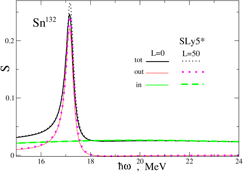
Figure 4: IVDR strength functions $S$ for vibrations of the nucleus ¹³²Sn as function of the excitation energy $\hbar\omega$ obtained for the Skyrme force SLy5^∗ pastore ; jmeyer with a value of $L=50$ MeV (dashed and dotted line) and with a zero value for $L$ (solid line). Out-of-phase and in-phase curves are shown separately for the main and the satellite excitation mode, respectively.

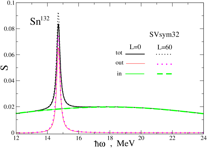
Figure 5: Same as Fig. 4 for the Skyrme force SVsym32 reinhardSV for a value of $L\approx 60$ MeV (dashed and dotted curves). For comparison the curves for $L=0$ are also shown.

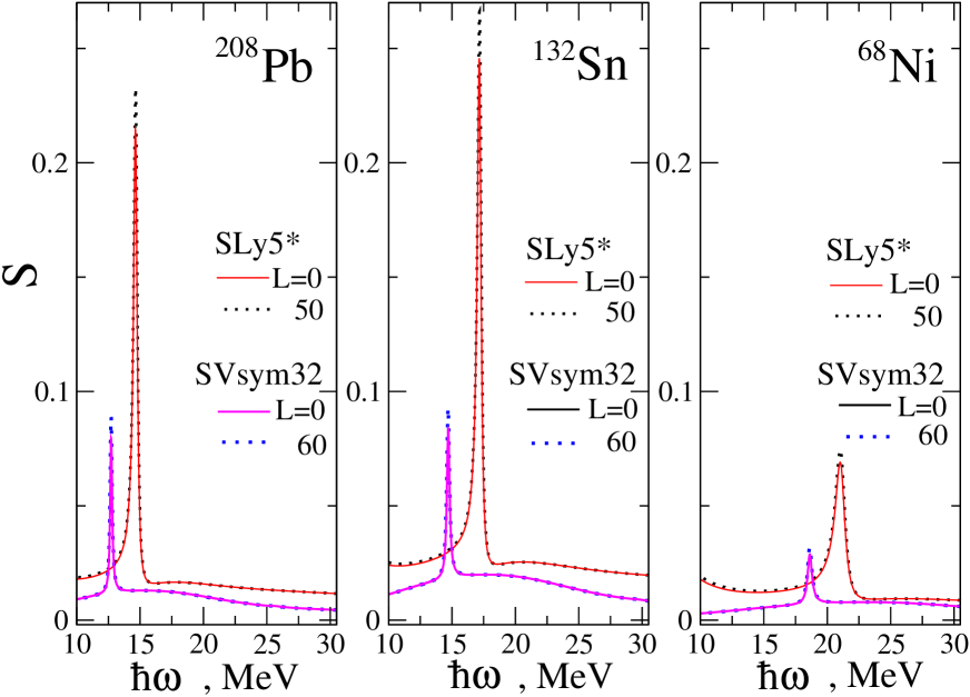
Figure 6: Total IVDR strength functions $S$ as function of the excitation energy $\hbar\omega$ obtained for different double magic nuclei with the Skyrme SLy5* (upper curve) and SVsym32 (lower curve) forces. The sensivity of the IVDR strength on the slope parameter $L$ at the main peak is seen to be very weak.

An investigation within the ES approach shows that the IVDR strength is split into a main peak which exhausts an essential part of the EWSR independent of the model and a satellite peak with a much smaller contribution into this quantity Figs. 4–6. Focusing on a more sensitive $k_{S}$ dependence of the IVDR satellite resonances, one may take now into account the slope $L$ dependence of the symmetry energy density (25) kievPygmy ; nester1 ; nester2 ; BMRps2015 . The total IVDR strength function, being respectively the sum of the “out-of-phase” $n=1$ and “in-phase” $n=2$ modes for the isovector- and isoscalar-like particle density vibrations in the nuclear volume, respectively (solid lines in Figs. 4 and 5 for the zero $L$, and dotted and dashed ones for the finite $L$), has a rather remarkable shape asymmetry BMRPhysScr2014 ; BMRps2015 ; BMRprc2015 . For SLy5^∗ (Fig. 4) and for SVsym32 (Fig. 5) one has the “in-phase” satellite to the right of the main “out-of-phase” peak. An enhancement to the left of the main peak for SLy5* is due to the increasing of the ”out-of-phase” strength (rare dotted curve in Fig. 4) at small energies because of appearance of a peak at the energy about a few MeV, in contrast to the SVsym32 case. The semiclassical FLDM calculations at the lowest $\hbar$ order should be improved here, for instance by taking into account the quantum effects as shell corrections within a more general POT belyaev ; BMps2013 . In the nucleus ¹³²Sn the IVDR energies of the two peaks do not change much with $L$ in both cases: $E_{1}=17$ MeV, $E_{2}=20$ MeV for SLy5^∗ (Fig. 4) and $E_{1}=15$ MeV, $E_{2}=18$ MeV for SVsym32 (Fig. 5). We find only an essential re-distribution of the EWSR contributions (normalized to 100% for the EWSR sum of the main and satellite peaks) [(63) for $S_{n}^{(1)}$] , This is due to a significant enhancement of the main “out-of-phase” peak with increasing $L$, $S^{(1)}_{1}=89$% and $S^{(1)}_{2}=11$% for SLy5^∗ (Fig. 4) and more pronounced EWSR distribution $S^{(1)}_{1}=76$% and $S^{(1)}_{2}=24$% for SVsym32 (Fig. 5) [cf. with the corresponding $L=0$ results: $S^{(1)}_{1}=88$% and $S^{(1)}_{2}=12$% for SLy5* and $S^{(1)}_{1}=73$% and $S^{(1)}_{2}=27$% for SVsym32]. These more precise calculations change essentially the IVDR strength distribution for the SV forces because of the smaller $c_{\rm sym}$ value as compared to other Skyrme interactions (Table 1). The collision relaxation time, $\mathcal{T}=4.3\cdot 10^{-21}$ s, is taken in Figs. 4– 6 in agreement with the IVGDR widths belyaev . Decreasing the relaxation time $\mathcal{T}$ by a factor of about 1.5 almost does not change the IVDR strength structure. However, we found a strong dependence on the relaxation time $\mathcal{T}$ in a wider region of $\mathcal{T}$ values. The “in-phase” strength component with a wide maximum does not depend much on the Skyrme force chaban ; reinhardSV ; pastore , the slope parameter $L$, and the relaxation time $\mathcal{T}$. We found also a regular change of the IVDR strength for different double-magic isotopes (Fig. 6). Besides of a big change for the energy (mainly because of $E_{1}$) and the strength [$S_{1}(\omega$)], one also obtains more asymmetry for ⁶⁸Ni than for the other isotopes. Calculations for nuclei with different mass $A$ were performed with the relaxation time $\mathcal{T}$ (61) where $\mathcal{T}_{0}=\mathcal{T}_{0\rm Pb}(208/A)^{1/3}$ with the parameter $\mathcal{T}_{0\rm Pb}=300$ MeV${}^{2}\cdot$s derived from the IVGDR width of ²⁰⁸Pb, in agreement with experimental data for the averaged $A$ dependence of the IVGDR widths ($\propto A^{-2/3}$). In this way the IVDR width becomes larger with decreasing $A$ as $A^{1/3}$, and at the same time, the height of peaks decreases. The $L$ corrections are also changing much in the same scale of all three nuclei.

The essential parameter of the Skyrme HF approach leading to the significant differences in the $k_{S}$ and $Q$ values is the constant $\mathcal{C}_{-}$ [(21) and Table 1]. Indeed, $\mathcal{C}_{-}$ is the key quantity in the expression for $Q$ (46) and the isovector surface-energy constant $k_{\rm S}$ [or $b_{\rm S}^{(-)}$ (40)], because $Q\propto 1/k_{\rm S}\propto 1/\mathcal{C}_{-}$ and $k_{\rm S}\propto\mathcal{C}_{-}$ BMRV . Concerning $k_{\rm S}$ and the IVDR strength structure, this is even more important than the $L$ dependence; though the latter changes significantly the isovector stiffness $Q$, and the neutron skin $\tau$. As seen in Table 1, the constant $\mathcal{C}_{-}$ is very different in absolute value and in sign for different Skyrme forces whereas $\mathcal{C}_{+}$ is almost constant. The isoscalar energy-density constant $b_{\rm S}^{(+)}$ is proportional to $C_{+}$ (III.3), in contrast to the isovector one. All of Skyrme parameters are fitted to the well-known experimental value $b_{\rm S}^{(+)}=17-19$ MeV while there are so far no clear experiments which would determine $k_{\rm S}$ well enough because the mean energies of the IVGDR (main peaks) do not depend very much on $k_{\rm S}$ for different Skyrme forces (the last three rows of Table 2). Perhaps, the low-lying isovector collective states are more sensitive but, at the present time, there is no careful systematic study of their $k_{\rm S}$ dependence. Another reason for so different $k_{\rm S}$ and $Q$ values might be due to difficulties in deducing $k_{\rm S}$ directly from the HF calculations because of the curvature and quantum effects. In this respect, the semi-infinite Fermi system with a hard plane wall might be more adequate for the comparison of the HF theory and the ETF effective surface approach. We have also to go far away from the nuclear stability line to subtract uniquely the coefficient $k_{\rm S}$ in the dependence of $b_{\rm S}^{(-)}\propto I^{2}=(N-Z)^{2}/A^{2}$, according to (40). For exotic nuclei one has more problems to derive $k_{\rm S}$ from the experimental data with enough precision. Note that, for studying the IVDR structure, the quantity $k_{S}$ is more fundamental than the isovector stiffness $Q$ because of the direct relation to the tension coefficient $\sigma_{-}$ of the isovector capillary pressure. Therefore, it is simpler to analyze the experimental data for the IVGDR within the macroscopic HD or FLD models in terms of the constant $k_{S}$. The quantity $Q$ involves also the ES approximation for the description of the nuclear edge through the neutron skin $\tau$ in (43). The $L$ dependence of the neutron skin $\tau$ is essential but not so dramatic in the case of SLy and SV forces (Table 2), besides of the SVmas08 forces with the effective mass 0.8. The precision of such a description depends more on the specific nuclear models vinas1 ; vinas2 ; vinas5 . On the other hand, the neutron skin thickness $\tau$, as the stiffness $Q$, is interesting in many aspects for an investigation of exotic nuclei, in particular, in nuclear astrophysics.

We emphasize that for specific Skyrme forces there exists an abnormal behavior of the isovector surface constants $k_{\rm S}$ and $Q$. It is related to the fundamental constant $\mathcal{C}_{-}$ of the energy density (21) but not to the derivative corrections to the symmetry energy density. For the parameter set T6 ($\mathcal{C}_{-}=0$) one finds $k_{\rm S}=0$ BMRV . Therefore, according to (46), the value of $Q$ diverges ($\nu$ is almost independent from $\mathcal{C}_{-}$ for SLy and SV forces; Table 2 and BMRV ; BMRPhysScr2014 ; BMRps2015 ). The isovector gradient terms which are important for the consistent derivations within the ES approach are also not included ($\mathcal{C}_{-}=0$) into the symmetry energy density in danielewicz1 ; danielewicz2 . In relativistic investigations vretenar1 ; vretenar2 ; vretenar3 of the pygmy modes and the structure of the IVGR distributions, the dependence of these quantities on the derivative terms has not been investigated so far. It therefore remains an interesting task for the future to apply similar semiclassical methods such as the ES approximation used in here also in relativistic models. Moreover, for RATP chaban and SV reinhard (like for SkI) Skyrme forces, the isovector stiffness $Q$ is even negative as $\mathcal{C}_{-}>0$ ($k_{\rm S}>0$) in contrast to other Skyrme forces. This would lead to an instability of the vibration of the neutron skin.

Table 2 shows also the coefficients $\nu$ of (46) for the isovector stiffness $Q$. They are almost constant for all SLy and SV Skyrme forces, unlike other forces BMRV . However, these constants $\nu$, being sensitive to the SO ($\beta$) dependence through (45), (44) and (41), change also with $L$ (Table 2). As compared to 9/4 suggested in myswann69 , they are significantly smaller in magnitude for the most of the Skyrme forces.

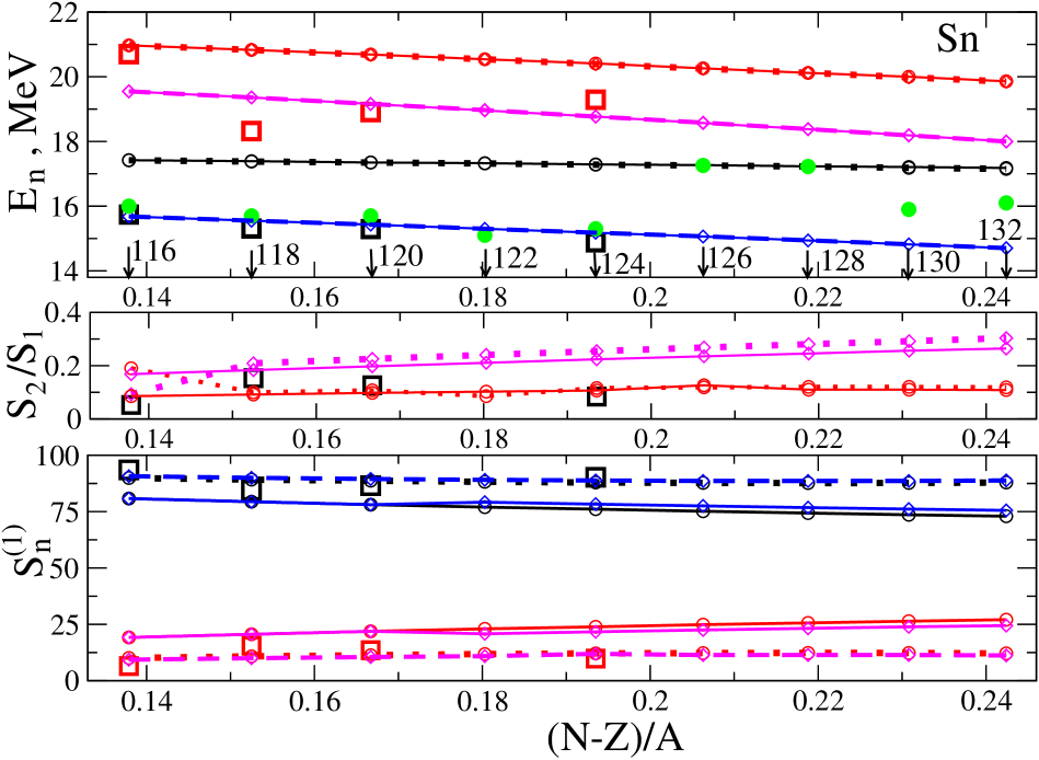
Figure 7: Energies and strength of the IVDR as function of the isospin asymmetry parameter $I=(N-Z)/A$ along the Sn isotopic chain from ¹¹⁶Sn to ¹³²Sn. Top: Energies $E_{1}$ and $E_{2}$ of the main and the satellite peak respectively. Open squares correspond to experimental data from integral cross sections (see the text) for the main peak (1, lower squares) and the satellite peak (2, upper squares). Large full circles represent experimental IVGDR data. Results obtained in theoretical calculations with the Skryme forces SLy5* (open circles and dotted curve) and the SVsym32 (open diamonds and dashed curve) are also shown, where the lower curves correspond to the main and the upper ones to the satellite peak. Middle: Ratio of stength of satellite versus main peak with the experimental IVDR data given by open squares. Theoretical results for SLy5* are shown by the solid curve with open circles (for $L=50$ MeV) and by tiny solid squares with open circles (for L=0), and for SVsym32 by the solid curve with open diamonds (for L=60 MeV) and the small solid squares with open diamonds (for $L=0$). Bottom: EWSR contributions of the main and the satellite peaks, normalized to 100%, as explained in the text, with the same notation as in the top of the figure (from BMRprc2015 ).

Figs. 6 and 7 show more systematic study for several isotopes and for the chain of the Sn isotopes, respectively. In Fig. 7, we compare the results of our calculations with the experimental data bermanSNexp ; vanderwoudeSNexp ; varlamovbook ; varlamovprep ; dietrichdata ; adrich . The latter were obtained by the fitting of the experimental strength curve for a given almost spherical Sn isotope by the two Lorenzian oscillator-strength functions as described in kolmagsh ; belyaev . It is always possible in the case of the asymmetric shapes of the strength curves with usual enhancement on right of the main peak, even in the case if the satellite cannot be distinguished well from the main peak in almost spherical nuclei (unlike the clear shoulders for the IVDRs in deformed ones). Each of these functions has three fitting parameters such as the inertia, stiffness and width of the peak belyaev . We found rather a good agreement of our ETF ES results with these experimental data for the energies, ratio of the strengths at the satellite to the main modes and the EWSR contributions.

More precise $L$-dependent calculations change essentially the IVDR strength distribution for the SV forces because of the smaller $c_{\rm sym}$ value as compared to other Skyrme interactions (Table 1). For ²⁰⁸Pb one obtains $E_{1}=15$ MeV, $S^{(1)}_{1}=91$% for the main peak and $E_{2}=17$ MeV, $S^{(1)}_{2}=9$% the satellite for SLy5^∗; and $E_{1}=13$ MeV, $S^{(1)}_{1}=83$% for the main peak and $E_{2}=16$ MeV, $S^{(1)}_{2}=17$% the satellite for SVsym32 forces. These calculations are qualitatively in agreement with the experimental results: $E_{1}=13$ MeV, EWSR ${}_{1}=98$% for the main peak and $E_{2}=17$ MeV, EWSR ${}_{2}=2$% the satellite. Descrepances might be related to the strong shell effects in this stable double magic nucleus which are neglected in the ETF ES approach.

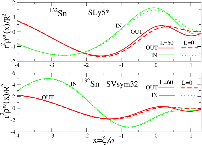
Figure 8: Main IVDR in-phase ($\delta\rho_{+}$, dots and thin solid line) and out-of-phase ($\delta\rho_{-}$, dashed and thick solid line) transition densities (multiplied by $(r/R)^{2}$) as function of the dimensionless distance coordinate $x=\xi/a\approx(r-R)/a$ for the satellite peak in the nucleus ¹³²Sn as obtained with the Skyrme interactions SLy5^∗ (upper part) and SVsym32 (lower part).

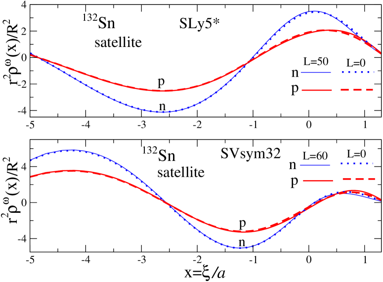
Figure 9: Same as Fig. 8, but for the IVDR neutron ($n$) and proton ($p$) transition densities (III.5) for the satellite energy $E=E_{2}$.

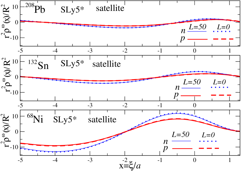
Figure 10: IVDR n-p transition densities $\rho^{\omega}(x)$, as in Fig. 9, but obtained with the Skyrme interaction SLy5* for three different nuclei, ²⁰⁸Pb (top), ¹³²Sn (middle) and ⁶⁸Ni (bottom), for the satellite peak. The sensitivity of our results with respect to the value of the derivative constant $L$ (in MeV) is shown to be small.

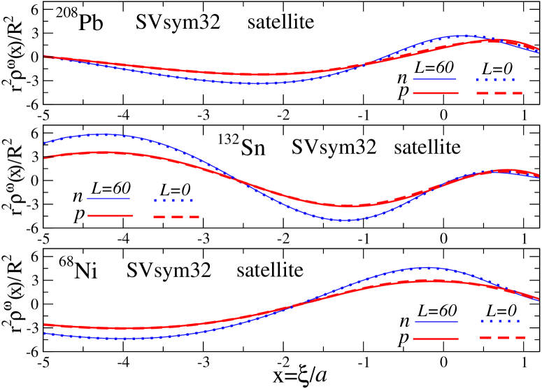
Figure 11: Same as Fig. 10 but for the Skyrme force SVsym32.

In Fig. 8 we show, in the case of the Skyrme forces SLy5* and SVsym32, the transition densities $\rho_{\mp}^{\omega}(x)$ of (55) for the “out”- of-phase (-) and the “in”- phase (+) modes of the volume vibrations at the excitation energy $E_{2}$ of the satellite. These are the key quantities for the calculation of the IVDR strengths, according to (53). The $L$ dependence is rather small, slightly notable mostly near the ES ($|x|\hbox{\kern 1.00006pt\lower 2.58334pt\hbox{$\sim$} \kern-11.19997pt\raise 2.58334pt\hbox{$<$} \kern 1.00006pt}1$). From Fig. 9, one finds a remarkable neutron versus proton excess near the nuclear edge for the same forces, which is however, very slightly depending on the slope parameter $L$. A small dependence of the transition densities on $L$ comes through the symmetry-energy constant $k_{\rm S}$ which is almost the same in modulus for these forces. We did not find a dramatic change of the transition densities with the sign of $k_{\rm S}$. Therefore, there is a weak sensitivity of the transition densities on $L$ through the energy $E_{2}$. We would have expected a stronger influence of the sign of $k_{\rm S}$ on the vibrations of the neutron skin rather than on the IVDR. This different sign leads to the opposite, stable and unstable, neutron skin vibrations. One observes also other differences between the upper (SLy5*) and the lower (SVsym32) panels in both figures: We find a redistribution of the surface-to-volume contributions of the transition densities for these two modes. In Figs. 10 and 11, one finds a considerable change of the neutron-proton transition densities for the same different isotopes for SLy5* and SVsym32 forces as in Fig. 6.

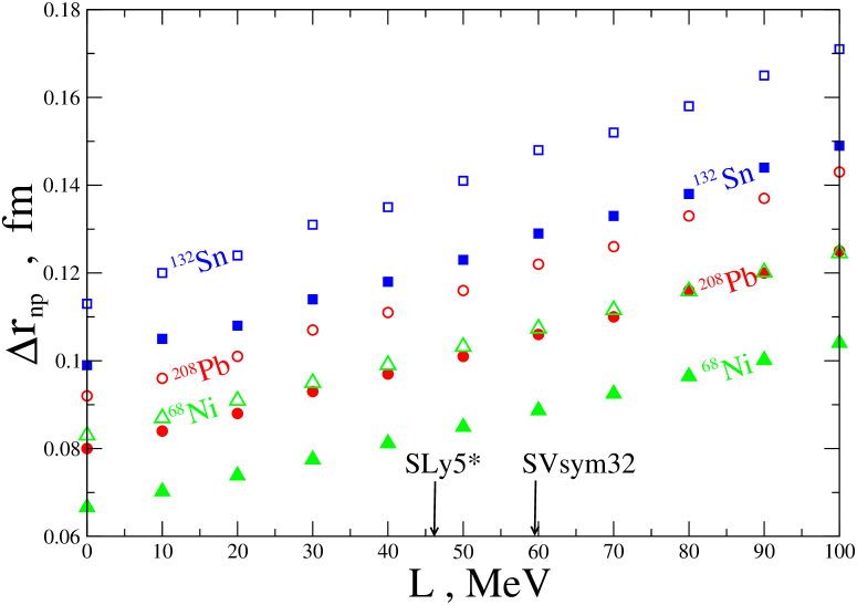
Figure 13: Neutron skin thickness, $\Delta r_{np}=\sqrt{3/5}(R_{n}-R_{p})$, as function of the asymmetry parameter $I$ with a comparison between experimental data obtained for the indicated nuclei from antiprotonic atoms with a droplet model fit taken from Ref. vinas5 .

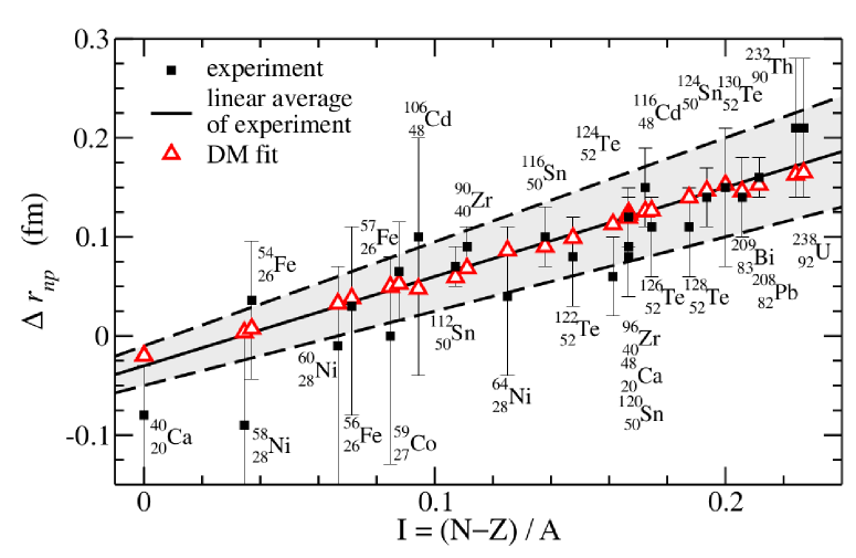
Figure 14: Neutron skin thickness, $\Delta r_{np}=\sqrt{3/5}(R_{n}-R_{p})$, as function of the asymmetry parameter $I$ with a comparison between experimental data obtained for the indicated nuclei from antiprotonic atoms with a droplet model fit taken from Ref. vinas5 .

The last three figures show theoretical (Figs. 12 and 13) and experimental (Fig. 14) evaluations of the neutron skin. Fig. 12 presents our calculations of the dimensionless skin $\tau/I$. Being independent of the specific properties of the nucleus, this quantity is universal. Fig. 13 shows the absolute values of the skin obtained from $\tau/I$ multiplying the mean-square evaluations of the nuclear radii by the factor $\sqrt{3/5}$ for an easy comparison with experimental data in Fig. 14. For ²⁰⁸Pb, one finds that the experimental values $\Delta r_{np}^{exp}=0.12-0.14$ fm in Fig. 14 (0.156${}_{-0.021}^{+0.025}$ fm, see rcnp ) are in good agreement with our calculations $\Delta r_{np}^{\rm theor}\approx 0.10-0.13$ fm within the ES approximation (the limits show values from SLy5* to SVsym32). For the isotope ¹²⁴Sn one obtains $\Delta r_{np}^{\rm theor}\approx 0.09-0.12$ fm, also in good agreement with experimental results (Fig. 14). For the isotope ¹³²Sn, we predict the value $\Delta r_{np}^{\rm theor}\approx 0.11-0.15$. Similarly, for ⁶⁰Ni and ⁶⁸Ni, one finds $\Delta r_{np}^{\rm theor}\approx 0.03-0.04$ (as in Fig. 14) and $0.08-0.11$, respectively.

Thus, in this section, the slope parameter $L$ was taken into account in the leading ES approximation in order to derive simple analytical expressions for the isovector particle densities and energies. These expressions were used for calculations of the surface symmetry energy, the neutron skin thickness and the isovector stiffness coefficients as functions of $L$. For the derivation of the surface symmetry energy and its dependence on the particle density we have to include main higher order terms in the parameter $a/R$. These terms depend on the well-known parameters of the Skyrme forces. Results for the isovector surface-energy constant $k_{\rm S}$, the neutron skin thickness $\tau$, and the neutron skin stiffness $Q$ depend in a sensitive way on the parameters of the Skyrme functional (especially on the parameter $\mathcal{C}_{-}$) in the gradient terms of the density in the surface symmetry energy [see (21)]. The isovector constants $k_{\rm S}$, $\tau$ and $Q$ depend also essentially on the slope parameter $L$, in addition to the SO interaction constant $\beta$. For all Skyrme forces, the isovector stiffness constants $Q$ are significantly larger than those obtained in earlier investigations. However, taking into account their $L$ dependence they come closer to the empirical data. It influences more on the isovector stiffness $Q$ and on the neutron skin $\tau$, than on the surface symmetry energy constant $k_{\rm S}$. The mean IVGDR energies and sum rules calculated in the macroscopic models like the FLDM kolmagsh ; BMVnpae2012 in Table 2 are in a fairly good agreement with the experimental data for most of the $k_{\rm S}$ values. As compared with the experimental data and other recent theoretical works, we found a rather reasonable two-peak structure of the IVDR strength within the FLDM. According to our results for the neutron and proton transition densities [Figs. 8, 9 and 10], we may interpret semiclassically the IVDR satellites as some kind of pygmy resonances endres on right of the main IVDR peak, though they might be of different nature from the so called Pygmy Dipole Resonances (PDRs) found on left of this peak vretenar1 ; vretenar2 ; ponomarev ; vretenar3 ; nester1 ; nester2 ; kievPygmy ; adrich ; wieland ; savran . The IVDR energies, sum rules and n-p transition densities obtained analytically within the semiclassical FLD approximation are sensitive to the surface symmetry energy constant $k_{{}_{\!S}}$ and the slope parameter $L$. Therefore, their comparison with the experimental data can be used for the evaluation of $k_{{}_{\!S}}$ and $L$. It seems helpful to describe them in terms of only few critical parameters, like $k_{\rm S}$ and $L$.

For further perspectives, it would be worthwhile to apply our results to calculations of the satellite resonances in the IVDR strength within the FLDM kolmagsh in a more systematic way. In this respect it is also interesting that the low-lying collective isovector states are expected to be even more sensitive to the values of $k_{\rm S}$ within the POT GMFprc2007 ; BMYijmpe2012 ; BMps2013 . More general problems of classical and quantum chaos in terms of the level statistics and Poincaré and Lyapunov exponents (see BMstatlevPRC2012 and references therein) might lead to a progress in studying the fundamental properties of collective dynamics like nuclear fission within the Swiatecki&Strutinsky macroscopic-microscopic model. Our approach is helpful also for further study of the effects in the surface symmetry energy because it gives analytical universal expressions for the constants $k_{\rm S}$, $\tau$ and $Q$ as functions of the slope parameter $L$ which do not depend on specific properties of nuclei as they are directly connected with a few critical parameters of the Skyrme interaction without any fitting.

IV COLLECTIVE EXCITATIONS
AS A SEMICLASSICAL RESPONSE

The collective dynamics of complex nuclei at low excitation energies, such as the vibration modes, can be described within several theoretical approaches bormot ; SOLbook1981 ; SOLbook1992 ; SOLQPMV-EPNP1985 ; migdalrev ; berborbro . One of the most powerful tools for its description is based on the response function theory bormot ; hofbook , in particular, within a semiclassical kinetic approach belyaev . This theory basically equivalent to the Random Phase Approximation (RPA) in the QPM SOLbook1981 ; SOLbook1992 ; SOLQPMV-EPNP1985 . The collective variables are introduced bormot ; hofbook explicitly as deformation parameters of a mean single-particle field. The nuclear collective excitations are parametrized in terms of the transport coefficients as the stiffness, the inertia, and the friction parameters through the adequate collective-response functions hofbook . The quantum formulation of this problem can be significantly simplified by using the SCM strut ; fuhi ; sclbook ; magNPAE2010 within the semiclassical approximation of the POT (Section II, and sclbook ; gutz ; bablo ; strumag ; magvvhof ). It would be worth to apply first the ideas of the SCM averaging and POT at a few leading orders in $\hbar$, as the ETF approach sclbook , for calculations of the smooth transport coefficients at low excitation energies.

The semiclassical derivations of the famous wall formula for the average friction, owing to collisions of particles of the perfect Fermi-gas with a slowly moving surface of the mean-field edge-like potential, were suggested in wall ; hatkoonran ; koonran , see also its derivations in abrdelmat ; yanbro ; hofivyam . The explicit analytical expressions of a smooth friction and inertia for the low-lying nuclear collective excitations within the semiclassical Gutzwiller path-integral approach to the POT gutz ; strumag at leading orders in $\hbar$, with the main focus on the consistency condition bormot ; hofbook ; ivhofpashyam between the variations of potential and particle number density, were considered in MGFyaf2007 ; belyaev ; MGFnpae2005 ; GMFprc2007 ; MGFnpae2008 . In the first Section IVA we derive the response function at small frequencies in terms of the averaged transport coefficients for studying the low-lying collective-vibration states.

IV.1 LOW-LYING COLLECTIVE EXCITATIONS OF NUCLEI

Following hofbook , we begin with a general response function formalism for transport coefficients in Section IVA1. They are expressed in terms of the semiclassical Green’s functions (Section II) and averaged in the phase space variables over many s.p. states near the Fermi surface in the simple case of a spherical cavity-like potential for a mean field at equilibrium in Section IVA2. The self-consistent relations between the transport coefficients and the coupling constant are presented in Section IVA3. The mean statistically vibration energies of the low-lying collective states and their EWSR contributions are derived in terms of analytical functions of nuclear particle number in Section IVA4. The reduced probabilities for the direct radiation decay of gamma quanta and the corresponding lifetimes of nuclei are discussed in Section IVA5. These analytical results for the low-lying quadrupole and octupole collective modes are compared with experimental data raman ; kibedi ; table in Section IVA6 and are summarized at the end of this section. Some details of the derivations are presented in Appendix B.

IV.1.1 Response theory and transport coefficients

Many-body collective excitations can be described in terms of the nuclear response to an external perturbation (51). For the symmetric nuclei, one has

$$V_{{\rm ext}}=\hat{\rm Q}\;q_{\rm ext}^{\omega}e^{-i\omega t}\;,$$ (67)

with a vibration amplitude, $q_{\rm ext}^{\omega}$, and the multipole s.p. operator, $\hat{\rm Q}=r^{\lambda}{\rm Y}_{\lambda 0}(\theta)$, ($\lambda\geq 2$) bormot . Its quantum average perturbation, $\delta\langle\hat{\rm{Q}}\rangle_{t}$, at time $t$ is calculated through the Fourier transform $\delta\langle\hat{\rm{Q}}\rangle_{\omega}$ obtained within the linear response theory bormot ; hofbook ; belyaev ,

$$\delta\langle\hat{\rm Q}\rangle_{\omega}=-\chi_{\rm QQ}^{\rm coll}(\omega)q_{\rm ext}^{\omega}\;,$$ (68)

where $\chi_{\rm QQ}^{\rm coll}(\omega)$ is the collective response function in the $Q$ mode. [In Section IV, $Q$ should not be confused with the neutron skin stiffness of the previous Section III.] The total Hamiltonian, $H_{\rm tot}=H+V_{\rm ext}$ at $q_{\rm ext}^{\omega}=0$, i.e. , $H$, depends on a collective variable $q$ defined as the time-dependent amplitude $q(t)$ of the potential $V(q)$. The vibrations of the axially-symmetric nuclear surface with a multipolarity $\lambda$ near the spherical shape can be described by

$$R(\theta,q)=R[1+q(t)Y_{\lambda 0}(\hat{r})]\;,$$

$$q(t)=q_{\omega}e^{-i\omega t}\;,\quad\hat{r}={\bf r}/r=\hbox{cos}\theta\;,$$ (69)

in the spherical coordinates, $Y_{\lambda 0}(\hat{r})$ is the spherical function of $\hat{r}$. The unperturbed quantities in dynamical variations are zero in this case. The consistency condition writes

$$\delta\langle\hat{\rm Q}\rangle_{\omega}=\kappa_{\rm QQ}\,\delta q_{\omega}\;,$$ (70)

where $\kappa_{\rm QQ}$ is the coupling constant, see Appendix B1. With help of the condition (70), the collective response bormot ,

$$\chi_{\rm{QQ}}^{{\rm coll}}(\omega)=\kappa_{\rm{QQ}}\frac{\chi_{\rm{QQ}}(\omega)}{\chi_{\rm QQ}(\omega)+\kappa_{\rm QQ}}\;,$$ (71)

is expressed in terms of the so called intrinsic response function, $\chi_{\rm QQ}(\omega)$, defined by

$$\delta\langle\hat{\rm Q}\rangle_{\omega}=-\chi_{\rm QQ}(\omega)\left(\delta q_{\omega}+q_{\rm ext}^{\omega}\right)\;.$$ (72)

One dominating peak in the collective strength function,

$$S(\omega)=\frac{1}{\pi}\;{\mbox{\rm Im}}\chi_{\rm QQ}^{\rm coll}(\omega)\;,$$ (73)

based on (71), at low excitation energies, $\hbar\omega_{\lambda}$, is assumed to be well separated from all other solutions of the secular equation $\chi_{\rm QQ}(\omega)+\kappa_{\rm QQ}=0$ for $\omega=\omega_{\lambda}$. See more detailed explanations of this approach for the case of another s.p. operator

$$\hat{{\rm F}}=(\partial V/\partial q)_{q=0}$$ (74)

with a mean field $V(q)$ in (B1) and for its applications to the collective nuclear dynamics in hofbook ; ivhofpashyam ; MGFyaf2007 ; belyaev . The corresponding oscillator response function in the q-mode, $\chi_{\rm qq}^{\rm coll}(\omega)$, can be conveniently written in an inverted approximate form hofbook ; ivhofpashyam :

$$\frac{1}{\chi_{\rm qq}^{\rm coll}(\omega)} = \frac{1}{\chi_{\rm qq}(\omega)}+\kappa_{\rm FF}\;$$ (75)

$$= -M_{\rm FF}\omega^{2}-i\gamma_{\rm FF}\omega+C_{\rm FF}\;,$$

where $\kappa_{\rm FF}$ is the coupling constant in the ${\rm F}$ mode, as shown in (B1),

$$\chi_{\rm qq}(\omega)=\frac{\chi_{\rm FF}(\omega)}{\kappa_{\rm FF}^{2}}=\frac{\chi_{\rm QQ}(\omega)}{\kappa_{\rm QQ}^{2}}\;.$$ (76)

According to the consistency conditions (70) and (B1), we used in (76) the approximate transformations between the quantities defined in different variables F and Q, corresponding to the s.p.  operators $\hat{F}$ and $\hat{Q}$. These transformations will be used for presentation of the results satisfying the consistency condition for variations of the nuclear potential, and the particle density in suitable units. Thus, according to (76), the inverse collective-response function for low frequencies $\omega$ is approximated by (75) through the response function of a damped harmonic oscillator, $\chi_{\rm qq}^{\rm coll}(\omega)$, with the stiffness of the nuclear free energy ${\cal F}$, $C_{\rm FF}\approx C_{\rm FF}(0)=\left({\partial^{2}{\cal F}/\partial q^{2}}\right)_{q=0}$, see hofbook , the friction $\gamma_{\rm FF}$ and the inertia $M_{\rm FF}$ parameters,

$$C_{\rm FF} = C_{\rm QQ}\;\frac{\kappa_{\rm FF}^{2}}{\kappa_{\rm QQ}^{2}}\;,$$

$$\gamma_{\rm FF} = \gamma_{\rm QQ}\;\frac{\kappa_{\rm FF}^{2}}{k_{\rm QQ}^{2}}\;,$$

$$M_{\rm FF} = M_{\rm QQ}\;\frac{\kappa_{\rm FF}^{2}}{\kappa_{\rm QQ}^{2}}\;.$$ (77)

The consistent transport coefficients $C_{\rm QQ}$, $\gamma_{\rm QQ}$ and $M_{\rm QQ}$ in a variable Q are related to the auxiliary intrinsic parameters $C_{\rm QQ}(0)$, $\gamma_{\rm QQ}(0)$ and $M_{\rm QQ}(0)$, as those of expansion of the intrinsic response function, $\chi_{\rm QQ}(\omega)$, in $\omega$ in the “zero-frequency limit”, $\omega\to 0$, for a slow collective motion hofbook ,

$$\chi_{\rm QQ}\left(\omega\right) = \chi_{\rm QQ}(0)-i\gamma_{\rm QQ}(0)\,\omega$$

$$- M_{\rm QQ}(0)\;\omega^{2}+\cdots\;,$$

$$\chi_{\rm QQ}(0) = -\kappa_{\rm QQ}-C_{\rm QQ}(0)\;.$$ (78)

Thus, for the transport parameters of the oscillator $\omega$-dependence in (75) and (IV.1.1), one has

$$C_{\rm QQ} = \left[1+C_{\rm QQ}(0)/\chi_{\rm QQ}(0)\right]C_{\rm QQ}(0)\;,$$

$$\gamma_{\rm QQ} = \left[1+C_{\rm QQ}(0)/\chi_{\rm QQ}(0)\right]^{2}\gamma_{\rm QQ}(0)\;,$$

$$M_{\rm QQ} = \left[1+C_{\rm QQ}(0)/\chi_{\rm QQ}(0)\right]^{2}\;$$ (79)

$$\times \left[M_{\rm QQ}(0)+\gamma_{\rm QQ}^{2}(0)/\chi_{\rm QQ}(0)\right].$$

With (76) and (IV.1.1), the poles of the oscillator response function of (75) are determined by the Newtonian equation of motion with a friction,

$$M_{\rm FF}\ddot{Q}+\gamma_{\rm FF}\dot{Q}-C_{\rm FF}=0,$$ (80)

which is helpful to clarify the physical meaning of the inertia $M_{{\rm FF}}$, the friction $\gamma_{{\rm FF}}$, and the stiffness $C_{{\rm FF}}$ of the collective motion.

The intrinsic response $\chi_{\rm{QQ}}(\omega)$ in equations (71) and (72) can be expressed in terms of the s.p.  Green’s function $G({\bf r}_{1},{\bf r}_{2};\varepsilon)$ (see (81) after the replace $\hat{Q}=\hat{F}$ magvvhof ; hofbook ).

$$\chi_{\rm QQ}(\omega)=\frac{d_{s}}{\pi}\int\limits_{0}^{\infty}{\hbox{d}\varepsilon\,n(\varepsilon)\int{\hbox{d}{\bf r}_{1}}}\int{\hbox{d}{\bf r}_{2}}\;$$ (81)

$$\times \hat{\rm Q}({\bf r}_{1})\,\hat{\rm Q}({\bf r}_{2})\,{\mbox{\rm Im}}G({\bf r}_{1},{\bf r}_{2};\varepsilon)$$

$$\times \left[\;\overline{G}\left({\bf r}_{1},{\bf r}_{2};\varepsilon-\hbar\omega\right)+G\left({\bf r}_{1},{\bf r}_{2};\varepsilon+\hbar\omega\right)\right],$$

where $n(\varepsilon)$ is the Fermi occupation numbers at the energy $\varepsilon$ for temperature $T$, $n(\varepsilon)=\{1+\hbox{exp}[(\varepsilon-\lambda)/T]\}^{-1}$, with the chemical potential, $\lambda\approx\varepsilon_{\rm F}$, $\varepsilon_{\rm F}$ is the Fermi energy. The factor of $d_{s}$ accounts again for the spin (spin-isospin) degeneracy by neglecting differences between the neutron and the proton potential wells (Section II). For the Green’s function $G({\bf r}_{1},{\bf r}_{2};\varepsilon)$ (bar above $G$ in (81) means the complex conjugation) we use the energy spectral representation,

$$G\left({\bf r}_{1},{\bf r}_{2};\varepsilon\right)=\sum_{i}\frac{\overline{\psi}_{i}({\bf r}_{1})\psi_{i}({\bf r}_{2})}{\varepsilon-\varepsilon_{i}+i\epsilon_{o}}\;,$$ (82)

where $\varepsilon_{i}$ is eigenvalues, $\psi_{i}$ eigenfunctions, and $\epsilon_{o}\rightarrow+0$ in the quantum mean-field approximation.

With the help of (81), the intrinsic response function, $\chi_{\rm QQ}(\omega)$, in the “zero-frequency limit” (IV.1.1) ($\omega\rightarrow 0$) can be expressed in terms of the Green’s function $G$ through the intrinsic parameters hofbook ; ivhofpashyam ,

$$\gamma_{\rm QQ}(0)=-i\left(\frac{\partial\chi_{\rm QQ}(\omega)}{\partial\omega}\right)_{\omega=0}\;$$ (83)

$$= \frac{d_{s}\hbar}{\pi}\int\limits_{0}^{\infty}\hbox{d}\varepsilon\;n(\varepsilon)\int\hbox{d}{\bf r}_{1}\int\hbox{d}{\bf r}_{2}\;\hat{\rm Q}\left({\bf r}_{1}\right)\,\hat{\rm Q}\left({\bf r}_{2}\right)\,$$

$$\times \frac{\partial}{\partial\varepsilon}\left[{\mbox{\rm Im}}\,G\left({\bf r}_{1},{\bf r}_{2};\varepsilon\right)\right]^{2},$$

$$M_{\rm QQ}(0)=\frac{1}{2}\,\,\left(\frac{\partial^{2}\chi_{\rm QQ}(\omega)}{\partial\omega^{2}}\right)_{\omega=0}\;$$ (84)

$$= \frac{d_{s}\hbar^{2}}{\pi}\,\int\limits_{0}^{\infty}\hbox{d}\varepsilon\,n(\varepsilon)\,\int\hbox{d}{\bf r}_{1}\,\int\hbox{d}{\bf r}_{2}\,\hat{\rm Q}({\bf r}_{1})\,\hat{\rm Q}({\bf r}_{2})\;$$

$$\times \rm{Im}\,G\left({\bf r}_{1},{\bf r}_{2};\varepsilon\right)\,\frac{\partial^{2}}{\partial\varepsilon^{2}}{\mbox{\rm Re}}\,G\left({\bf r}_{1},{\bf r}_{2};\varepsilon\right).$$

Using the spectral representation (82) for the Green’s function $G$ one reduces equivalently equation (84) to the well-known cranking model inertia in the mean-field limit in the ${\rm F}$ mode ($\epsilon_{0}\to+0$) hofbook ,

$$M(0)=d_{s}\hbar^{2}{\sum_{ij}}^{\prime}\,\frac{n_{i}-n_{j}}{(\varepsilon_{j}-\varepsilon_{i})^{3}}\,|<i|\hat{{\rm F}}|j>|^{2},$$ (85)

where $~{}<i|\hat{{\rm F}}|j>~{}$ is the matrix element of the operator $\hat{{\rm F}}$ (74); see, e.g. , hofbook . The prime means that the diagonal terms, $~{}\varepsilon_{i}=\varepsilon_{j}$, are excluded in these summations.

For the collective response function at the low-lying excitation energies, (68), with the help of (75) and (76), one has

$$\chi_{\rm QQ}^{\rm coll}\left(\omega\right)=\frac{\kappa_{\rm QQ}^{2}}{-M_{\rm FF}\omega^{2}-i\gamma_{\rm FF}\omega+C_{\rm FF}}\;,$$ (86)

where the inertia $M_{\rm FF}$, the friction $\gamma_{\rm FF}$, and the stiffness $C_{\rm FF}$ are given by (IV.1.1), (IV.1.1), (83) and (84). The coupling constant $\kappa_{\rm QQ}$ is defined by the consistency condition (70), see Appendix B1. According to (86) for the response function $\chi_{\rm QQ}^{\rm coll}(\omega)$ ($\lambda=2,3,\cdots$) , the strength function $S_{\lambda}(\omega)$ (73) for the first lowest peak is given by

$$S_{\lambda}(\omega)\!=\!\frac{\kappa_{\rm QQ}^{2}}{\pi}\frac{\gamma_{\rm FF}\,\omega}{\left(-M_{\rm FF}\omega^{2}+C_{\rm FF}\right)^{2}+\gamma_{\rm FF}^{2}\omega^{2}}\;.$$ (87)

Substituting this strength function into its moments,

$$S_{\lambda}^{(l)}=\hbar^{{\it l}+1}\int\limits_{0}^{\infty}\hbox{d}\omega\;\omega^{{\it l}}\;S_{\lambda}(\omega)\;,$$ (88)

${\it l}=0,1,...$, one can evaluate the probability distributions for excitations of the low-lying collective states.

IV.1.2 Semiclassical EGA for transport coefficients

The trace of the first term $G_{{\rm CT}_{0}}({\bf r}_{1},{\bf r}_{2};\varepsilon)$, ${\bf r}_{2}\to{\bf r}_{1}$, in (II.1) corresponds to a smooth level density, $g_{\rm ETF}(\varepsilon)$, and the ETF particle number conservation writes sclbook ; bablo

$$A = d_{s}\int\limits_{0}^{\infty}\hbox{d}\varepsilon\,\widetilde{n}(\varepsilon)\,g_{\rm ETF}(\varepsilon)$$ (89)

$$\approx d_{s}\left[\frac{2(k_{F}R)^{3}}{9\pi}-\frac{(k_{F}R)^{2}}{4}+\frac{2k_{F}R}{3\pi}\right]\;,$$

where $\widetilde{n}$ is the occupation number averaged by using the Strutinsky smoothing strut ; fuhi , $k_{F}$ is the Fermi momentum in units of $\hbar$, $k_{F}=\sqrt{2m\varepsilon_{F}/\hbar^{2}}$ for billiards. Equation (89) determines the semiclassical parameter $k_{F}R$ as function of the particle number $A$. The second and third terms in the very right approximation in (89) for spherical cavity-like mean fields, which becomes exact for the infinitely deep square-well potential, account for important surface and curvature corrections to the first main volume component, respectively. The temperature corrections, $\sim(T/\varepsilon_{F})^{2}$, might be taken into account through the usual Sommerfeld expansion, too, see below and hofbook ; MGFyaf2007 . We shall omit such small corrections because the applications will be applied to the low-lying collective excitations at zero temperature.

As well known strumag ; sclbook , due to $\hbar$ in the denominators of exponents of (II.1) in the oscillating terms of the Green’s function traces, their semiclassical expansions in $\hbar$, or in dimensionless parameter, $\hbar/S_{\rm CT}\sim 1/k_{F}R$, converge after averaging in $k_{F}R$, for instance, over a large enough interval of the particle number $A$ through the radius $R$ in accordance with (89). The Strutinsky averaging strut ; fuhi ; magNPAE2010 ; migdalrev with a Gaussian width $\widetilde{\Gamma}$, which covers at least a few major shells in energy spectrum, see Appendix B1, leads to the local (${\bf r}_{2}\to{\bf r}_{1}$) averaged quantities; in particular, the smooth level and particle density, and free energy. According to (83), (84), the unlocal (${\bf r}_{2}\neq{\bf r}_{1}$) contributions into the ETF transport coefficients become also important. Therefore, we need more extended statistical averaging in the phase space (energy and spatial coordinate) variables, as in the semiclassical (moreover, local hydrodynamical) derivations within the many-body particle density or Green’s function formalism kadbaym ; kolmagpl .

The averaged semiclassical inertia, ${\tilde{M}}_{\rm QQ}(0)$, and friction, $\widetilde{\gamma}_{\rm QQ}(0)$, parameters can be found by substitution of the trajectory expansion of Green’s function (II.1) into (83) and (84),

$$\widetilde{M}_{\rm QQ}(0)=\frac{d_{s}\hbar^{2}}{\pi}\,\sum_{\rm CT,CT^{\prime}}\langle\int\limits_{0}^{\infty}\hbox{d}\varepsilon n(\varepsilon)$$ (90)

$$\times\int\hbox{d}{\bf r}_{1}\!\int\hbox{d}{\bf r}_{2}\,\hat{\rm Q}\left({\bf r}_{1}\right)\hat{\rm Q}\left({\bf r}_{2}\right)$$

$$\times {\mbox{\rm Im}}\,G_{\rm CT}\left({\bf r}_{1},{\bf r}_{2};\varepsilon\right)\,\,\frac{\partial^{2}}{\partial\varepsilon^{2}}{\mbox{\rm Re}}\,G_{\rm CT^{\prime}}\left({\bf r}_{1},{\bf r}_{2};\varepsilon\right)\rangle_{\rm av}\;,$$

$$\widetilde{\gamma}_{\rm QQ}(0)=\frac{d_{s}\hbar}{\pi}\sum_{\rm CT,CT^{\prime}}\langle\int\limits_{0}^{\infty}\hbox{d}\varepsilon\;n(\varepsilon)$$ (91)

$$\times\int\hbox{d}{\bf r}_{1}\,\int\hbox{d}{\bf r}_{2}\;\hat{\rm Q}\left({\bf r}_{1}\right)\,\hat{\rm Q}\left({\bf r}_{2}\right)$$

$$\times \frac{\partial}{\partial\varepsilon}\left[{\mbox{\rm Im}}\,G_{\rm CT}\left({\bf r}_{1},{\bf r}_{2};\varepsilon\right)\;{\mbox{\rm Im}}\,G_{\rm CT^{\prime}}\left({\bf r}_{1},{\bf r}_{2};\varepsilon\right)\right]\rangle_{\rm av}\;,$$

where the angle brackets $<\cdots>_{\rm av}$ mean an averaging over the phase space coordinates, including the SCM averaging in $k_{F}R$ variable with a width related to $\widetilde{\Gamma}$, as mentioned above. In order to calculate analytically these quantities, we need to distinguish the two limit cases GMFprc2007 ; MGFyaf2007 :

(i) the nearly local part, $S_{\rm CT}({\bf r}_{1},{\bf r}_{2};\varepsilon_{F})/\hbar\approx k_{F}{\cal L}_{\rm CT}\hbox{\kern 1.00006pt\lower 2.58334pt\hbox{$\sim$} \kern-11.19997pt\raise 2.58334pt\hbox{$<$} \kern 1.00006pt}1\;$,

and

(ii) nonlocal contributions, $k_{F}{\cal L}_{\rm CT}>>1\;$,

where ${\cal L}_{\rm CT}$ is the length of the CT in the edge-like potential wells. We emphasize that the averaging over phase-space variables (the spatial coordinates, and the energy spectrum) leads to the nearly local approximation (NLA) (i) for the inertia (90) and friction (91) coefficients, in contrast to the case (ii). For the case (i), the partial SCM averaging in $k_{F}R$ (for instance, in nuclear sizes $R$ or particle numbers $A$ for the constant $k_{F}$ fixed by the particle density of infinite matter) ensures a convergence of the semiclassical expansions of smooth quantities in $1/k_{F}R$ within the ETF model sclbook . The strong energy-dependent exponential factor of (II.1), $\hbox{exp}(iS_{\rm CT}(\varepsilon)/\hbar)$, for $\hbar\to 0$ serves appearance of the damping factor, $\propto\hbox{exp}[-({\cal L}_{\rm CT}\Gamma/4R)^{2}]$ after such averaging with a width of the Gaussian weight function, $\Gamma\hbox{\kern 1.00006pt\lower 2.58334pt\hbox{$\sim$} \kern-11.19997pt\raise 2.58334pt\hbox{$>$} \kern 1.00006pt}(2\div 4)k_{F}R\,\hbar\Omega/2$, see Appendix B3. This averaging, corresponding to the $2\div 4$ distances between the major shells in energy spectrum, $\hbar\Omega\approx\varepsilon_{F}/A^{1/3}=7\div 10~{}$ MeV for heavy nuclei, $A=200\div 50$, respectively, removes shell effects, like in the ETF both level and particle densities strut ; fuhi ; sclbook ; MGFyaf2007 ; MGFnpae2008 . The most important contribution is coming then from the trajectory, CT$=$CT^′=CT₀, see Fig. 1, with a short length smaller than a few wave lengths, $1/k_{F}$, ${\cal L}_{{\rm CT}0}=s=|{\bf r}_{2}-{\bf r}_{1}|\hbox{\kern 1.00006pt\lower 2.58334pt\hbox{$\sim$} \kern-11.19997pt\raise 2.58334pt\hbox{$<$} \kern 1.00006pt}1/k_{F}<<R$, at large semiclassical parameter, $k_{F}R>>1$.

As in kadbaym ; kolmagpl ; MGFyaf2007 , it is convenient now to transform the variables $\{{\bf r}_{1},{\bf r}_{2}\}$ to the Wigner coordinates $\{{\bf r},{\bf s}\}$,

$${\bf r}=({\bf r}_{1}+{\bf r}_{2})/2,\qquad\qquad{\bf s}={\bf r}_{2}-{\bf r}_{1},$$ (92)

to simplify calculations of the inertia $\widetilde{M}_{\rm QQ}(0)$ (90) and the friction $\widetilde{\gamma}_{\rm QQ}(0)$ (91) by separating a slow motion of particles in variable ${\bf r}$ and their fast motion in ${\bf s}$. With the transformation (92) and exchange of the energy and spatial integrations, in the case (i), one has

$$\widetilde{M}_{\rm QQ}(0)=\frac{d_{s}\hbar^{2}}{\pi}$$ (93)

$$\times \langle\int\hbox{d}{\bf r}\,\int\hbox{d}{\bf s}\,\hat{Q}\left({\bf r}+\frac{{\bf s}}{2}\right)\,\hat{Q}\left({\bf r}-\frac{{\bf s}}{2}\right)\;$$

$$\times \int\limits_{0}^{\infty}\hbox{d}\varepsilon\,n(\varepsilon)\;{\mbox{\rm Im}}\,G_{{\rm CT}_{0}}\left({\bf r}+\frac{{\bf s}}{2},{\bf r}-\frac{{\bf s}}{2};\varepsilon\right)$$

$$\times \frac{\partial^{2}}{\partial\varepsilon^{2}}{\mbox{\rm Re}}\,G_{{\rm CT}_{0}}\left({\bf r}+\frac{{\bf s}}{2},{\bf r}-\frac{{\bf s}}{2};\varepsilon\right)\rangle_{\rm av},$$

$$\widetilde{\gamma}_{\rm QQ}(0)=\frac{d_{s}\hbar}{\pi}$$ (94)

$$\times \langle\int\hbox{d}{\bf r}\int\hbox{d}{\bf s}\,\,\hat{Q}\left({\bf r}+\frac{{\bf s}}{2}\right)\,\hat{Q}\left({\bf r}-\frac{{\bf s}}{2}\right)\;$$

$$\times \!\!\!\int\limits_{0}^{\infty}\hbox{d}\varepsilon\;n(\varepsilon)\frac{\partial}{\partial\varepsilon}\left[{\mbox{\rm Im}}\,G_{{\rm CT}_{0}}\left({\bf r}+\frac{{\bf s}}{2},{\bf r}-\frac{{\bf s}}{2};\varepsilon\right)\right]^{2}\rangle_{\rm av}\;.$$

As shown in Appendix B3, for small enough length $s$ of the trajectory CT₀, $s/R<<1$ in the case (i), the corresponding component $G_{{\rm CT}_{0}}$ of Green’s function (II.1) in (93), (94) in terms of the new integration variables $\{{\bf r},{\bf s}\}$ is reduced approximately to its simple analytical form (II.1) belyaev ; MGFyaf2007 . Formally, $G_{0}$ coincides with the well-known Green’s function for a free particle motion bablo ; hatkoonran ; koonran ; strumag .

The internal integral over $\varepsilon$ in (93) and (94) can be taken analytically within the nearly local approximation (II.1). For the analytical integrations over the Wigner coordinates ${\bf r}$ and ${\bf s}$, the integrands depending on $k_{F}s$ in (93), (94) are simplified by means of averaging in the phase space variables. As shown in Appendix B3, using the approximation (II.1) one may identically transform the expressions for the inertia $M_{\rm QQ}(0)$, the friction $\gamma_{{\rm QQ}}(0)$ and the isolated susceptibility $\chi_{\rm QQ}(0)$ to sums of local (volume) terms and their small nonlocal (surface) corrections. The integrands, proportional linearly to the nonlocal (correlation-like) components depending on $k_{F}R$, are zeros within the considered approach (i). The inertia terms expressed linearly through the correlation function, $<Q({\bf r}+{\bf s}/2)Q({\bf r}-{\bf s}/2)-Q^{2}({\bf r})>_{\rm av}$, averaged in phase-space variables, are neglected like in the derivations of the hydrodynamic model (HDM) starting from a many-body system of strong interacting particles. A more general statistical principle of the weakness of correlations is used usually in the semiclassical derivations of the kinetic equations with integral collision terms, by separating a slow motion along the mean coordinate ${\bf r}$ within nearly local condition (i) from a fast dynamics in the relative coordinate ${\bf s}$ in terms of its collisional correlations kadbaym ; kolmagpl ; belyaev . Such correlation-like functions are concentrated at small $s$ of the order of a few wave lengths, $1/k_{F}$, as explained in Appendix B3. The transport coefficients are simplified by averaging in fast oscillations of functions of the relative coordinate ${\bf s}$ at a given mean coordinate ${\bf r}$. The integrations over angles of vectors ${\bf s}$ and ${\bf r}$ can be approximately performed analytically in the NLA (i), see Appendix B3.

Thus, the main contribution into remaining integrals over ${\bf s}$ and ${\bf r}$ in (93) and (94) within the NLA (i) is coming from $s\hbox{\kern 1.00006pt\lower 2.58334pt\hbox{$\sim$} \kern-11.19997pt\raise 2.58334pt\hbox{$<$} \kern 1.00006pt}1/k_{F}$ for $1/k_{F}R<<1$. The major terms can be found in the perfect local case when a smooth product of the multipole operators in these equations can be approximately taken off the integral over ${\bf s}$ at ${\bf s}=0$, according to the property of the phase-space averaging of the correlation functions mentioned above. For the main local approximation in the case (i), after the integration over $\varepsilon$ (or corresponding $kR$), one may take also analytically the integrals over ${\bf s}$ and ${\bf r}$ in (93) and (94), see Appendix B3. As the final result, for $\lambda\geq 2$ one finally arrives at the inertia,

$$\widetilde{M}_{\rm QQ}(0)=\frac{d_{s}m^{3}R^{2\lambda+6}}{12\pi\hbar^{4}}\;f_{\lambda}^{(3)},$$ (95)

the friction,

$$\widetilde{\gamma}_{\rm QQ}(0)=\frac{d_{s}m^{2}R^{2\lambda+4}}{2\pi^{2}\hbar^{3}}\,f_{\lambda}^{(1)},$$ (96)

and the isolated susceptibility,

$$\widetilde{\chi}_{\rm QQ}(0)=\frac{d_{s}mR^{2\lambda+2}\;k_{F}R}{2\pi^{2}\;\hbar^{2}}\,f_{\lambda}^{(0)},$$ (97)

see Appendix B, respectively. Here, $f_{\lambda}^{(n)}$ are the integrals over the dimensionless radial variable,

$$f_{\lambda}^{(n)}=\int\limits_{0}^{1}\hbox{d}\wp\;\wp^{2\lambda+2}\;\left(\wp+1\right)^{n},$$ (98)

$$f_{\lambda}^{(0)}=\frac{1}{2\lambda+3},\quad f_{\lambda}^{(1)}=\frac{4\lambda+7}{2(\lambda+2)(2\lambda+3)}\;,$$

$$f_{\lambda}^{(3)}=\frac{(4\lambda+9)[(4\lambda+9)^{2}-7]}{4(\lambda+2)(\lambda+3)(2\lambda+3)(2\lambda+5)}\;,$$ (99)

where $n=0,1,2,...,\quad\wp=r/R$. The next high-order terms of expansion of the product of multipole operators in powers of the dimensionless variable $s/R$ lead to some small surface corrections, relatively $\sim 1/k_{F}R$, at large particle number A. In particular, it is shown that the next order curvature corrections, $\sim 1/(k_{F}R)^{2}$, for a given large $k_{F}R$ can be neglected within the considered almost local (TF) approximation in the case (i). Notice that more important surface ($\sim 1/k_{F}R$) and curvature ($\sim 1/(k_{F}R)^{2}$) corrections are originated from those of the ETF relationship between $k_{F}R$ and particle number A (89). The derivation of the surface and curvature corrections are considered in Appendix B shown for shortness only at the very end of Section IV.1.3. All of them will be discussed in last Sections IV.1.4–IV.1.6.

For evaluation of the contributions (ii) of longer trajectories, the Gutzwiller expansion (II.1) with (II.1) valid for the isolated classical paths, fails because we have to account for a continuous symmetry of the spherical Hamiltonian, e.g. , appearance of the axially-symmetric degenerated families of planar POs with their points fixed inside of the spherical reflection boundary strumag . For such a family, due to the integration over its continuous parameter, the amplitude of the Green’s function term, $G_{\rm CT}$, in expansion (II.1) over trajectories CTs is enhanced in order of $(k_{F}{\cal L}_{\rm CT})^{1/2}$ (or $\hbar^{-1/2},~{}k_{F}{\cal L}_{\rm CT}>>1$), as compared to (II.1) and (II.1) strumag ; magosc . For the case of higher classical degeneracy ${\cal K}$ (Section II) the CTs closed in the phase space, i.e. , PO families, yield the contributions into the Green’s function amplitude enhanced by the factor $(k_{F}{\cal L}_{\rm CT})^{{\cal K}/2}$ for billiards, or $[S_{\rm CT}(\varepsilon_{F})/\hbar]^{{\cal K}/2}$ for potentials with the edge diffuseness as RPLP in MKApanSOL1 . For the nondiagonal (CT$\neq$CT^′) contributions (ii) into the integrals over ${\bf r}_{2}$ (or ${\bf s}$ in the ${\bf r}$, ${\bf s}$ coordinates) in (90) and (91) with parameter $\Gamma$ of the SCM averaging, much smaller than that related to the distance between major shells $\hbar\Omega$, the leading terms in semiclassical parameter $k_{F}R$ are the POs, according to the stationary phase conditions magvvhof . These nondiagonal terms provide, through the stationary phase (PO) conditions provide mainly the shell (nonlocal) corrections to the inertia $M_{\rm QQ}(0)$, the friction $\gamma_{\rm QQ}(0)$, and the isolated susceptibility $\chi_{\rm QQ}(0)$ MGFnpae2008 . They will be discussed in details in further publications. In following, within this Section IVA, we shall consider only the smooth transport coefficients, and therefore, for simplicity, the tilde above them will be omitted everywhere.

IV.1.3 Coupling constants and transport coefficients

As shown in hofbook ; GMFprc2007 ; MGFyaf2007 , the consistent collective-transport coefficients $\gamma_{\rm QQ}$, $M_{\rm QQ}$ and $C_{\rm QQ}$ of (IV.1.1) differ from their auxiliary “intrinsic” parameters $\gamma_{\rm QQ}(0)$ (96), $M_{\rm QQ}(0)$ (95) and $C_{\rm QQ}(0)$, see also $\chi_{\rm QQ}(0)$ (97), in the low frequency expansion (IV.1.1) by small semiclassically corrections,

$$\frac{C_{\rm QQ}(0)}{\chi_{\rm QQ}(0)}=\frac{C_{\rm FF}(0)}{\chi_{\rm FF}(0)}\sim\,\frac{1}{(k_{F}R)^{2}}<<1\;,$$ (100)

as shown in hofbook ; MGFyaf2007 , and

$$\frac{\gamma^{2}_{\rm QQ}(0)}{\chi_{\rm QQ}(0)M_{\rm QQ}(0)}=\frac{6}{\pi}\,\frac{[f_{\lambda}^{(1)}]^{2}}{f_{\lambda}^{(0)}\,f_{\lambda}^{(3)}}\,\frac{1}{k_{F}R}$$

$$\approx\frac{1}{k_{F}R}<<1\;,$$ (101)

in contrast to the corresponding result within the approach of MGFyaf2007 . Therefore, in the following derivations, one may neglect the curvature corrections (100) in (IV.1.1) but keep (IV.1.3) for the surface terms ($\sim 1/k_{F}R$),

$$C_{\rm QQ} \approx C_{\rm QQ}(0),\quad\gamma_{\rm QQ}\approx\gamma_{\rm QQ}(0)\;,$$

$$M_{\rm QQ} \approx M_{\rm QQ}(0)+\gamma_{\rm QQ}^{2}(0)/\chi_{\rm QQ}(0)\;.$$ (102)

For calculations of the response function $\chi_{\rm QQ}^{\rm coll}(\omega)$ (86), one has to transform the transport coefficients $\gamma_{\rm QQ}$, $M_{\rm QQ}$ and $C_{\rm QQ}$ from the variable $Q$ related to the s.p. operator $\hat{Q}$ to another variable associated with the operator $\hat{{\rm F}}$ by using (IV.1.1) bormot ; hofbook ; MGFyaf2007 . The coupling constants $\kappa_{\rm FF}$ and $\kappa_{\rm QQ}$ appearing both in the transformation equations (IV.1.1) are given by

$$\kappa_{\rm FF} = -\frac{32\overline{\rho}b_{\rm V}KR^{4}}{675b_{\rm S}r_{0}}$$ (103)

$$\approx -\frac{8\;KR}{225\pi\;b_{\rm S}r_{0}}\;b_{\rm V}A$$

and

$$\kappa_{\rm QQ} = \rho R^{L+3}\;,$$

$$\rho = \overline{\rho}\left(1+\frac{6b_{\rm S}r_{0}}{KR}\right)\approx\overline{\rho}\;,$$ (104)

with the parameters $b_{\rm V}$, $K$, $r_{0}~{}~{}$ ($\overline{\rho}$) of infinite nuclear matter defined in Section IIA. The energy surface constant, $b_{\rm S}=b^{(+)}_{\rm S}$, is given by (III.3). For the typical nuclear parameters, the surface-tension particle-density correction in (IV.1.3) inside of nucleus is small relatively for heavy nuclei, $6b_{\rm S}r_{0}/KR\approx 6b_{\rm S}/KA^{1/3}<<1$, in the ES approximation strmagbr ; strmagden .

Substituting (IV.1.1), (103), (IV.1.3), (95) and (96) into (IV.1.1) for the consistent transport coefficients in the Thomas-Fermi approach, one approximately finds

$$M_{\rm FF}=6\pi^{2}Lf_{\lambda}^{(3)}\;\rho\;\left(\frac{16b_{v}\;KR}{2025\varepsilon_{F}\;b_{\rm S}r_{0}}\right)^{2}$$

$$\times\frac{(k_{F}R)^{4}}{A}\;M_{\rm irr}\;,\qquad M_{\rm irr}=\frac{3AmR^{2}}{4\lambda\pi}\;,$$ (105)

$$\gamma_{\rm FF} = \frac{1}{2}\;f_{\lambda}^{(1)}\;\left(\frac{32b_{\rm V}\;KR}{675\varepsilon_{F}\;b_{\rm S}r_{0}}\right)^{2}\gamma_{\rm wf}\;,$$

$$\gamma_{\rm wf} = \frac{3}{4}\hbar\rho k_{F}R^{4}\;,$$ (106)

where $M_{\rm irr}$ is the irrotational flow inertia of the hydrodynamical LDM (HDM) bormot , and $\gamma_{\rm wf}$ is the wall formula wall ; koonran re-derived in MGFyaf2007 for the operator $\hat{\rm F}$ of (B1) in the NLA (i). They both are used below as convenient units. Notice, the convergence of the expansions in semiclassical parameter, $1/k_{F}R$, and leading terms (IV.1.3) for $M_{\rm FF}$ and (IV.1.3) for $\gamma_{\rm FF}$ survive owing to the Strutinsky averaging in $k_{F}R$ [see (B3)] with a Gaussian width $\widetilde{\Gamma}$ corresponding at least to a few major shells $\hbar\Omega$ of the energy spectrum strut ; fuhi ; sclbook . The in-compressibility $K$ and the surface energy constant $b_{\rm S}$ appear in these equations in terms of the same semiclassical and leptodermous parameter, $1/k_{F}R\sim a/R\propto b_{\rm S}/KA^{1/3}$ ($k_{F}a\sim k_{F}r_{0}\sim 1$, $R=r_{0}A^{1/3})$ up to a number constant, through (103) for the coupling constant $\kappa_{\rm FF}$, see Appendix B1 and Section III. Such general common properties of the ETF and liquid-droplet models based both on expansion in small parameter $a/R$ were found, for instance, within the ES approach strmagbr ; strmagden .

However, the ETF inertia (IV.1.3) is much larger than that of irrotational flow, $M_{\rm irr}$, in terms of the parameter $k_{F}R\sim A^{1/3}>>1$,

$$\frac{M_{\rm FF}}{M_{\rm irr}} = \overline{M}_{\rm FF}A\;,$$ (107)

$$\overline{M}_{\rm FF} \approx 0.036,\quad\mbox{for}\quad\lambda=2\;,$$

$$\overline{M}_{\rm FF} \approx 0.043,\quad\mbox{for}\quad\lambda=3\;.$$ (108)

In these evaluations of the relative inertia for the symmetric Fermi-system of $A$ nucleons we used the nuclear data mentioned above ($b_{\rm V}=16$ MeV, $K=220$ MeV, $\overline{\rho}=0.16$ fm^-3, $b_{\rm S}=18$ MeV). The Fermi energy $\varepsilon_{F}$ is determined through the Fermi wave number $k_{F}$ by particle density of infinite nuclear matter, $\overline{\rho}=2k_{F}^{3}/3\pi^{2}$, as usually in the Thomas-Fermi model sclbook . For particle number $A=100\div 200$, the inertia values $M_{\rm FF}$ are larger than the irrotational flow one by factor of about $4\div 7$ for the quadrupole (L=2) and almost $4\div 9$ for the octupole (L=3) vibrations, respectively. Note that an inertia enhancement with respect to the quantity $M_{\rm irr}$ was found in kolkon within the stochastic cranking model.

Taking into account the unlocal surface corrections (B3) of (93) and (IV.1.3) of (IV.1.1) ($\propto\gamma_{\rm QQ}^{2}(0)$), which are both small relatively as $1/k_{F}R\sim A^{-1/3}$, for the inertia $M_{\rm FF}$, see also (IV.1.1), up to small negligibly curvature corrections of (100), one obtains

$$M_{\rm FF}=\frac{\pi\rho m^{3}R^{2L+6}}{2\hbar^{4}k_{F}^{3}}\,\frac{\kappa^{2}_{\rm FF}}{\kappa^{2}_{\rm QQ}}\;$$ (109)

$$\times \left(f_{\lambda}^{(3)}+\frac{\zeta_{\lambda}}{\pi\;k_{F}R}\right)\left(1+\frac{6[f_{\lambda}^{(1)}]^{2}}{\pi k_{F}Rf_{\lambda}^{(0)}\;f_{\lambda}^{(3)}}\right)\;.$$

Here, $\kappa_{\rm FF}$ and $\kappa_{\rm QQ}$ are the coupling constants (103) and (IV.1.3) [(B.7) and (B1)] completed by small surface and curvature corrections, respectively; $f_{\lambda}^{(n)}$ are given by (98) and (IV.1.2); $\zeta_{\lambda}=\zeta_{\lambda}^{(1)}+\zeta_{\lambda}^{(2)}>0$, where $~{}\zeta_{2}^{(1)}=-3f_{2}^{(2)}=-127/84$, $~{}\zeta_{2}^{(2)}=1279/576~{}$ for $~{}\lambda=2~{}$, $~{}\zeta_{3}^{(1)}=-3f_{3}^{(2)}=-199/165$, and $~{}\zeta_{3}^{(2)}=67031/42240~{}$ at $~{}\lambda=3$, $f_{\lambda}^{(2)}=(8\lambda^{2}+32\lambda+31)/[(\lambda+2)(2\lambda+3)(2\lambda+5)]$, see Appendix B, (B3) and (B3).

For the stiffness, $C_{\rm FF}$, at leading order of expansion in $A^{-1/3}$ within the ES approximation strmagbr ; strmagden ; GMFprc2007 ; MGFyaf2007 , as for the coupling constant, $\kappa_{\rm FF}$, one has the values of the HDM for the vibration multipolarity $\lambda$ bormot ,

$$C_{\rm FF}\equiv C_{\lambda}^{(S)}+C_{\lambda}^{\rm(Coul)}\;.$$ (110)

The surface component of the HD stiffness,

$$C_{\lambda}^{({\rm S})}=\frac{b_{\rm S}}{4\pi r_{0}^{2}}\,(\lambda-1)(\lambda+2)\,R^{2}\;,$$ (111)

is complemented by the Coulomb term along the $\beta$-stability line bormot ; bormot1 ,

$$C_{\lambda}^{({\rm Coul})} = -\frac{3\,(\lambda-1)}{2\pi\,(2\lambda+1)}\,\frac{Z^{2}e^{2}}{R}\;,$$

$$Z = \left[\frac{A}{2+3e^{2}\,A^{2/3}/10r_{0}J}\right]\;,$$ (112)

where $Ze$ is the charge of nucleus. The square brackets in (IV.1.3) mean the integer part of number, and $J$ is the coefficient of symmetry term in the nuclear binding energy (Section III). The approximation $C_{\rm FF}\approx C_{\rm FF}(0)$ up to small semiclassically curvature corrections, $\sim A^{-2/3}$, see (100), was used here as in (109) hofbook ; GMFprc2007 ; MGFyaf2007 .

IV.1.4 Vibration energies and sum rules

The energies of the collective vibration modes are determined by poles of the response function (86) with the inertia $M_{\rm FF}$ (IV.1.3), the friction $\gamma_{\rm FF}$ (IV.1.3), the stiffness $C_{\rm FF}$ (110), and the coupling constant $\kappa_{\rm QQ}$ (IV.1.3). These poles are given by

$$\omega_{\pm}=\varpi\left(\pm\sqrt{1-\eta_{\rm FF}^{2}}-i\eta_{\rm FF}\right),$$ (113)

where

$$\varpi = \sqrt{\frac{C_{\rm FF}}{M_{\rm FF}}}\;,$$

$$\eta_{\rm FF} = \frac{\gamma_{\rm FF}}{2\sqrt{M_{\rm FF}\;C_{\rm FF}}}\;.$$ (114)

Subscript “$FF$” in $\eta_{\rm FF}$ will be omitted within this section for simplicity. According to (IV.1.3), (IV.1.3), (111) and (IV.1.3), for the effective damping parameter $\eta$, see (IV.1.4), one finds $\eta\hbox{\kern 1.00006pt\lower 2.58334pt\hbox{$\sim$} \kern-11.19997pt\raise 2.58334pt\hbox{$<$} \kern 1.00006pt}$ 0.4 and 0.2 for $\lambda=2$ and $3$, respectively. The last estimates were obtained for the same nuclear parameters shown above at $A\hbox{\kern 1.00006pt\lower 2.58334pt\hbox{$\sim$} \kern-11.19997pt\raise 2.58334pt\hbox{$<$} \kern 1.00006pt}200$ with accounting for surface and curvature corrections. As seen from these estimates, the collective motion under consideration is underdamped, $\eta<1$, for any realistic particle numbers, $A\hbox{\kern 1.00006pt\lower 2.58334pt\hbox{$\sim$} \kern-11.19997pt\raise 2.58334pt\hbox{$<$} \kern 1.00006pt}200$. Note that the residue interaction was zero from the very beginning in (82) for the Green’s function $G$, $\epsilon_{0}=+0$. The averaging over $k_{F}R$ which guarantees a convergence of smooth transport coefficients in the semiclassical expansion over $\hbar$ (or $1/k_{F}R$ in dimensionless units), leads to a finite friction coefficient, $\gamma_{\rm FF}$, or an effective damping constant $\eta$, as formally with $\epsilon_{o}\neq 0$ in (82). More precisely, it takes place for the formal averaging with Lorentzian weight function, see bablo ; koonran . However, as shown in this and two next sections, the influence of the effective damping parameter $\eta$ on calculations of the excitation energies, transitions probabilities, and EWSR contributions can be neglected in the following derivations.

Neglecting now by small $\eta^{2}$ term in the real part of (113) for calculations of the smooth low-lying collective vibration energy, $\hbar\omega=\hbar{\mbox{\rm Re}}\;\omega_{+}\approx\hbar\varpi$, from (113), (IV.1.4), (IV.1.3) and (110), at $\lambda\geq 2$ one approximately obtains

$$\hbar\omega_{\lambda} = \frac{D_{\lambda}}{A}\;,$$

$${\cal D}_{\lambda} = \overline{D}_{\lambda}\left(1+\frac{C_{\lambda}^{({\rm Coul})}}{C_{\lambda}^{({\rm S})}}\right)^{1/2},$$ (115)

$$\overline{D}_{\lambda} = \frac{75\,b_{\rm S}\varepsilon_{F}}{4\pi b_{\rm V}K}$$ (116)

$$\times \sqrt{\frac{3\varepsilon_{F}b_{\rm S}(\lambda-1)(\lambda+2)}{f_{\lambda}^{(3)}}}\;.$$

For nuclear parameters mentioned above, the constant $\overline{\cal D}_{\lambda}\;$, independent of the particle number A, is given approximately by $\overline{D}_{2}=100$ MeV and $\overline{D}_{3}=180$ MeV. With the Coulomb corrections of (IV.1.4), these constants become slightly almost linearly decreasing functions of A within the interval about $A=100\div 200$. For this A interval they are modified approximately to the values $D_{2}=90\div 70$ MeV, and $D_{3}=170\div 150$ MeV, respectively, see (111) and (IV.1.3).

We may now evaluate the EWSR $S_{\lambda}^{(1)}$ for contribution of the first low-lying excitation, see the integral (88) for ${\it l}=1$ with the strength function $S_{\lambda}(\omega)$ (87). Using now the even parity of its integrand, one can extend the low integration limit to $-\infty$ and integrate over $\omega$ by the residue method in complex plane of $\omega$. Closing the integration contour in lower plane of $\omega$ we calculate the contributions of the two poles $\omega=\omega_{\pm}$ inside of this closed contour. Finally, for the EWSR of the low-lying collective excitation, one finds [see also (88), (IV.1.3) and (IV.1.3)]

$$S_{\lambda}^{(1)} = \frac{\hbar^{2}\;\kappa_{\rm QQ}^{2}}{2M_{\rm FF}}$$ (117)

$$= \frac{M_{\rm irr}}{M_{\rm FF}}\,S_{\lambda,{\rm cl}}\;,$$

where

$$S_{\lambda,{\rm cl}}=\frac{\hbar^{2}\;\kappa_{\rm QQ}^{2}}{2M_{\rm irr}}=\frac{3\lambda;\varepsilon_{F}}{4\pi\,(k_{F}R)^{2}}\;AR^{2\lambda}.$$ (118)

This $S_{\lambda,{\rm cl}}$ appears to be exactly the same as the contribution of the low-lying peak in the HDM of the irrotational flow in a classical liquid droplet. It is equivalent to the EWSR estimation independent of the model, see (6.179a) in bormot . The ratio of the inertias, $M_{\rm irr}/M_{\rm FF}$, in (117) is given by (IV.1.3). Note that the last equation in (117) recalls the EWSR relation (6.183) of bormot . Thus, we may evaluate the relative contribution of the low-lying collective state into this total EWSR estimation $S_{\lambda,{\rm cl}}$, see (117) with (IV.1.3) and (107),

$$\frac{S_{\lambda}^{(1)}}{S_{\lambda,{\rm cl}}} = \frac{\overline{S}_{\lambda}^{(1)}}{A}\;,$$

$$\overline{S}_{\lambda}^{(1)} = \frac{2}{\lambda f_{\lambda}^{(3)}}\;\left(\frac{225\,\varepsilon_{F}b_{\rm S}k_{F}r_{0}}{8\pi b_{\rm V}K}\right)^{2},$$ (119)

with constants $\overline{S}_{2}^{(1)}\approx 7$ and $\overline{S}_{3}^{(1)}\approx 6$ for the same nuclear parameters. For $A\sim 100\div 200$ one has a small relatively EWSR contribution of the low-lying collective excitations in the framework of the ETF model. According to (107), this is obviously because of small values of the ratio of inertia parameters, $M_{\rm irr}/M_{\rm FF}$, for large particle numbers A. It is in contrast to the HDM where the first low-lying peak exhausts erroneously 100% of the EWSR $S_{\lambda,{\rm cl}}$ independent of the model bormot . By this reason, the ETF approach to the collective nuclear vibrations is much improved with respect to the HDM results: In addition to the low-lying collective states, one has a possibility for the giant multipole-resonance contributions which mainly exhaust the EWSR.

The small relatively surface and curvature corrections can be taken into account in the vibration energies (IV.1.4) and sum rules (117) through (109) for the inertia and (89) for the ETF relationship of the parameter $k_{F}R$ to the particle number $A$, see Appendices B1 [(B.7) and (B1)] and B3. The last kind of the relative surface ($\sim A^{-1/3}$) and curvature ($\sim A^{-2/3}$) corrections from (89) yield the major contribution into the $A$-systematics of the vibration energies (IV.1.4) for large $A$,

$$\hbar\omega_{\lambda}=\frac{D_{\lambda}}{A}\left(1-\frac{w^{(s)}_{\lambda}}{A^{1/3}}+\frac{w^{(c)}_{\lambda}}{A^{2/3}}\right),$$ (120)

where $D_{\lambda}$ is defined in (IV.1.4) and (116),

$$w^{(s)}_{\lambda} = \left(\frac{9\pi}{8}\right)^{2/3}\approx 2.3\;,$$

$$w^{(c)}_{\lambda} = 3\left(\frac{8}{9\pi}\right)^{2/3}\approx 1.3\;.$$ (121)

Similarly, from (117) one obtains the EWSR ratio:

$$\frac{S_{\lambda}^{(1)}}{S_{\lambda,{\rm cl}}}=\frac{\overline{S}_{\lambda}^{(1)}}{A}$$

$$\times\left(1-\frac{2w^{(s)}_{\lambda}}{A^{1/3}}+\frac{[w_{\lambda}^{(s)}]^{2}+2w_{\lambda}^{(c)}}{A^{2/3}}\right),$$ (122)

where $\overline{S}_{\lambda}$ is the constant independent of the particle numbers A in (IV.1.4). Other surface and curvature components do not contribute almost due to their smallness or mutual compensations. Note that the surface corrections decrease essentially both vibration energies $\hbar\omega_{\lambda}$ (120), and EWSR contributions $S_{\lambda}^{(1)}$ (IV.1.4) for large sufficiently values of particle numbers, $A=100\div 200$, because of positive sign of the dominating surface correction constant $w_{\lambda}^{(s)}$, Eq.  (IV.1.4), that is important especially for the EWSR.

IV.1.5 Transport probabilities and direct radiation decay

The radiation decay of the low-lying collective states can be considered as a direct emission of the gamma-quantum from nucleus with the semiclassical description of a charged system within our ETF approach. A similar process for the case of the direct radiation decay of isoscalar giant multipole resonances by using the Landau-Vlasov approach with the macroscopic boundary conditions (Appendix A2) within the framework of the semiclassical description of a nuclear system was studied in magpl . For the probability of the transitions per unit of time with the electric radiation of the gamma-quantum energy $\varepsilon_{\gamma}$ at multipolarity $\lambda$, one has bormot1

$$W(E\lambda,I_{1}\rightarrow I_{2})=\frac{8\pi(\lambda+1)}{\lambda[(2\lambda+1)!!]^{2}\hbar}$$ (123)

$$\times \left(\frac{\varepsilon_{\gamma}}{\hbar c}\right)^{2\lambda+1}B(E\lambda,I_{1}\rightarrow I_{2})\;.$$

Here, $I_{1}$ and $I_{2}$ are the spins of the initial and the final states, $B(E\lambda,I_{1}\rightarrow I_{2})$ is the reduced probability,

$$B(E\lambda,I_{1}\rightarrow I_{2})$$

$$=\sum_{\mu M_{2}}|\langle I_{2}M_{2}|{\cal M}(E\lambda,\mu)|I_{1}M_{1}\rangle|^{2}\;,$$ (124)

$\mu$ and $M_{2}$ are the projections of the gamma-quantum spin $\lambda$ and the angular momentum of a final nuclear state $I_{2}$, respectively, and

$$\mathcal{M}(E\lambda,\mu)=\frac{eZ}{A}\;\int\hbox{d}{\bf r}\rho({\bf r})\;r^{\lambda}Y_{\lambda\mu}(\theta,\varphi)\;.$$ (125)

The effective charge factor can be approximately put one for the isoscalar collective excitations with $\lambda\geq 2$.

The quantum reduced probability $B(E\lambda,0\rightarrow\lambda)$ (IV.1.5) can be evaluated through the zero moment $S_{\lambda}^{(0)}$ (88) of the strength function $S_{\lambda}(\omega)$ (87). Taking into account the conservation equations for the energy, $\varepsilon_{\gamma}=\hbar\omega_{\lambda}$, and the angular momentum, $I_{2}=\lambda$ ($I_{1}=0$) in the direct nuclear-gamma decay bormot1 ; magpl for the zero moment of (88) by using a handbook one obtains

$$S_{\lambda}^{(0)} = \frac{\hbar\;\kappa_{\rm QQ}^{2}}{2\pi M_{\rm FF}\omega_{\lambda}\;\sqrt{1-\eta^{2}}}$$ (126)

$$\times \mbox{arccot}\left[\frac{2\eta^{2}-1}{2\eta\sqrt{1-\eta^{2}}}\right]$$

$$= \frac{\hbar\;\kappa_{\rm QQ}^{2}}{2M_{\rm FF}\,\omega_{\lambda}}\left[1-\frac{2\eta}{\pi}+{\cal O}\left(\eta^{2}\right)\right],$$

where $M_{\rm FF}$, $\kappa_{\rm QQ}$ and $\eta=\eta_{\rm FF}$ are given by (109), (B1) and (IV.1.4), respectively, see also (IV.1.3) and (110), $\eta<1/\sqrt{2}$. As shown in the previous section, the contribution of $\eta$ terms is really small enough for particle numbers $A\hbox{\kern 1.00006pt\lower 2.58334pt\hbox{$\sim$} \kern-11.19997pt\raise 2.58334pt\hbox{$<$} \kern 1.00006pt}200$ and all multipolarities $\lambda\geq 2$ under consideration such that one may neglect all $\eta$ corrections in (126). The averaged probability $B(E\lambda,0\rightarrow\lambda)$ (IV.1.5) can be then approximated semiclassically within the ETF model,

$$B(E\lambda,0\rightarrow\lambda)\approx B_{\rm scl}(E\lambda,0\rightarrow\lambda)$$

$$\!=\!(2\lambda+1)\left(\frac{eZ}{A}\right)^{2}S_{\lambda}^{(0)}\!\approx\!(2\lambda+1)\left(\frac{eZ}{A}\right)^{2}\!$$

$$\times\frac{\hbar\;\kappa_{\rm QQ}^{2}}{2M_{\rm FF}\,\omega_{\lambda}}\;.$$ (127)

The degeneracy factor $2\lambda+1$ was accounted because of the additional summation over the projections $M_{2}$ of the final angular momentum $I_{2}=\lambda$ in (IV.1.5) with (125), as compared to the simplest multipole operator for the isoscalar excitations of $A$ nucleons, $\int\hbox{d}{\bf r}\rho({\bf r})\;r^{\lambda}Y_{\lambda 0}(\theta)$, considered in the previous sections. The factor $(eZ/A)^{2}$ must be also taken into account in the last two equations in (IV.1.5), see (IV.1.5), (125), and (6.61), (6.182) of bormot . The semiclassical energy of the low-lying collective state, $\hbar\omega_{\lambda}$, was derived in Section IV.1.4, see the first equation in (IV.1.4) and its approximations (IV.1.4) and (120), as applied for the considered direct radiation decay like in magpl . Other denotations are the same as in the sum rule (117). Thus, from comparison of the transition probability (IV.1.5) and the EWSR (117) modified with the operator (125), one has the following approximate relationship between the probability (IV.1.5) and the corresponding sum rule bormot ; magpl :

$${S}_{\lambda,{\rm scl}} \equiv (2\lambda+1)\;\left(\frac{eZ}{A}\right)^{2}\;S_{\lambda}^{(1)}$$ (128)

$$= \hbar\omega_{\lambda}B_{\rm scl}(E\lambda,0\rightarrow\lambda).$$

According to (128), (117), (107) and (IV.1.4), the reduced probability $B(E\lambda)$, for example, for the radiation process $\lambda\to 0$ in units of the s.p. estimation bormot1 mainly writes

$$\frac{B_{\rm scl}(E\lambda)}{B_{\rm s.p.}(E\lambda)}\approx\frac{\hbar^{2}\lambda(3+\lambda)^{2}}{6mr_{0}^{2}\;D_{\lambda}\overline{M}_{\rm FF}}\left(\frac{Z}{A}\right)^{2}A^{1/3}\;.$$ (129)

As seen from this simple evaluation, the particle dependence of the reduced probability $B_{\rm scl}(E\lambda)$ divided by the factor $(Z/A)^{2}$ in the s.p. units is roughly proportional to a large semiclassically parameter $A^{1/3}$. In these derivations we used the approximate relation (IV.1.3) of the proton number $Z$ to the total particle number $A$. Taking into account also the coefficient in front of the $A^{1/3}$ dependence (129), one obtains even larger magnitude for this relative probability, $~{}\approx 80\div 130~{}$ for the quadrupole and $~{}\approx 80\div 90~{}$ for the octupole low-lying collective states at large particle numbers, $A=100\div 200$, respectively. With the main surface and curvature corrections of (IV.1.4) and (120), owing to the ones of the ETF relationship (89) between $k_{F}R$ and $A$, these quantities are decreased with respect to their local (volume) approximation, $~{}\approx 50\div 70~{}$ for $\lambda=2$ and $~{}\approx 50\div 60$ for $\lambda=3$. Thus, in any case the quadrupole and octupole electric transitions within our semiclassical model are the well pronounced sufficiently collective excitations.

For the mean semiclassical lifetime with respect to the direct gamma decay, one has

$$t_{\lambda,\rm scl}=W_{\rm scl}^{-1}(E\lambda,\lambda\to 0)\;$$ (130)

$$\propto \omega_{\lambda}^{-(2\lambda+1)}B_{\rm scl}^{-1}(E\lambda,\lambda\rightarrow 0)$$

$$\propto (A/eZ)^{2}A^{2(2\lambda+1)/3}.$$

With the semiclassical ETF probability per unit of time $W_{\rm scl}(E\lambda,\lambda\to 0)$ (123) corresponding to the reduced probability $B_{\rm scl}(E\lambda,\lambda\rightarrow 0)$ (IV.1.5), one obtains $t_{2,\rm scl}\approx 80\div 1100$ and $t_{3,\rm scl}\approx(17\div 1100)\cdot 10^{6}$ ps for the quadrupole and octupole low-lying collective vibration states within the same particle number interval. We accounted for the main surface and curvature corrections which increase significantly lifetimes $t_{\lambda,\rm scl}$ (130). In these evaluations we neglected the corrections owing to the conversion processes which become important for much smaller excitation energies.

IV.1.6 Comparison with experimental data

Figures 15 and 16 show the local Thomas-Fermi approach to the low-lying collective quadrupole, $\hbar\omega_{2}$, and octupole, $\hbar\omega_{3}$, excitation energies; see (IV.1.4) with (110) for the stiffness, $C_{\rm FF}$, and (IV.1.3) for the inertia, $M_{\rm FF}$, without surface and curvature corrections, as compared to the experimental data raman and kibedi , respectively, see also table . The calculations are performed for the following nuclear parameters: $\overline{\rho}=0.16$ fm^-3 ($r_{0}=1.14$ fm), $b_{\rm V}=16$ MeV, $b_{\rm S}=18$ MeV, $K=220$ MeV, $J_{\rm sym}=30$ MeV (Section III). The almost spherical nuclei with quadrupole deformations, $q_{2}\hbox{\kern 1.00006pt\lower 2.58334pt\hbox{$\sim$} \kern-11.19997pt\raise 2.58334pt\hbox{$<$} \kern 1.00006pt}0.05$, are selected from these experimental data table ; plugor ; plugorkad ; MGFyaf2007 . The Thomas-Fermi results for smooth vibration energies are significantly improved with respect to the hydrodynamic (HD) behavior with the same stiffness $C_{\rm FF}$ (110) but the irrotational flow inertia, $M_{\rm irr}$ of (IV.1.3), especially for the quadrupole case.

More complete ETF approach (IV.1.4), (110) and (109) with accounting for the surface and curvature corrections of the function, $k_{F}R(A)$, found from (89) and those of the inertia $M_{\rm FF}$, (109), (B.7) and (B1), see Appendices B1 and B3, are shown as ETF curves in Figs. 15 and 16. As expected, the comparison with experimental data, except for several doubly-closed-shell (magic) nuclei which appear above the regular A-systematics, is essentially improved by these corrections, mainly for smaller particle numbers A. The Coulomb stiffness component becomes important for larger A. The reason of better agreement of the ETF approach, as compared to the HD model, with experimental data for nonmagic nuclei can be explained by larger ETF inertias $M_{\rm FF}$, see (107), than that of the irrotational flow, $M_{\rm irr}$, for heavy nuclei. As seen from these Figures, the explicit analytical formula (120) (ETFA, dashed), where the only surface and curvature corrections in the $k_{F}R(A)$ ETF dependence (89) were taken into account, is a good asymptotics for large particle numbers, $A\hbox{\kern 1.00006pt\lower 2.58334pt\hbox{$\sim$} \kern-11.19997pt\raise 2.58334pt\hbox{$>$} \kern 1.00006pt}40$. We should emphasize that this asymptotics versus the TF and ETF curves shows importance of namely these corrections, as compared to all other ones.

Figs. 17 and 18 show the semiclassical reduced probability,

$$~{}~{}~{}B_{\rm scl}(E\lambda,0\rightarrow\lambda)=(2L+1)B_{\rm scl}(E\lambda,\lambda\rightarrow 0)$$

[see (IV.1.5)], related to the zero moment of the strength function (73), see also (88) at ${\it l}=0$, versus experimental data table ; raman ; kibedi for the quadrupole, $0^{+}\to 2^{+}$, and the octupole, $0^{+}\to 3^{-}$, electric collective transitions in the low-lying energy region for the same nearly spherical nuclei. The logarithmic scale is used in order to show this comparison in a wide region of particle numbers. As seen from these Figures, one has a good agreement between the averaged semiclassical reduced transition probabilities and the global behavior of experimental data raman ; kibedi (besides of magic nuclei). The surface and curvature correction effects measured by differences between TF and ETF curves are in fact smaller than both of them in comparison with the HD values. Our semiclassical smooth A-systematic results look better versus the experimental data than that of the HDM. The agreement between the full ETF (thin solid) and the analytical asymptotics ETFA (thick dashed) with the main surface and curvature corrections coming from (89) is really perfect for almost all particle numbers, except for very small particle numbers, $A\hbox{\kern 1.00006pt\lower 2.58334pt\hbox{$\sim$} \kern-11.19997pt\raise 2.58334pt\hbox{$<$} \kern 1.00006pt}40$. As shown in Section IV.1.5, the comparison in Figs. 17 and 18 is a basis in experimental and theoretical analysis of the direct radiation decay of the low-lying collective states. For instance, the quadrupole lifetime $t_{\lambda,\rm{scl}}$ (130) (Fig. 19) associated with the direct processes of the gamma-quantum emission bormot1 ; magpl are reasonable in order of the magnitude as compared to the experimental data raman . As seen from comparison of the frequent dashed (ETF^∗) and solid lines (ETF) in Figs. 17 and 18, one may really neglect the $\eta$ corrections of (IV.1.5) which arise from the averaging procedure. The dynamic surface effects improve our semiclassical lifetime $t_{\lambda,\rm scl}$ (130) towards the experimental data table ; raman .

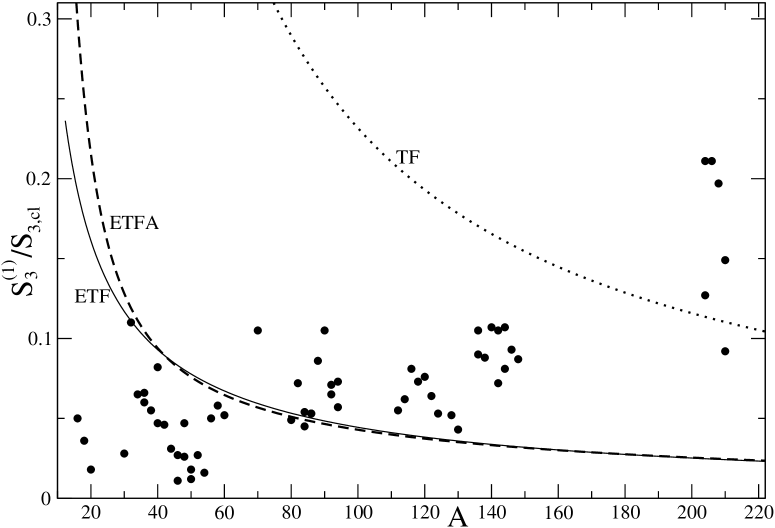
Figure 21: Same as Fig. 20 but for the octupole EWSR $S_{3}^{(1)}$ in units of $S_{3,{\rm cl}}$, with solid circles showing $\hbar\omega_{3}B(E3)$ with the experimental $\hbar\omega_{3}$ and $B(E3)$ from kibedi ; table .

One of the most important characteristics of the low-lying collective states is their energy weighted sum rule contribution (117) into the total value $S_{\lambda,{\rm cl}}$ (118), independent of the model bormot , see Figs. 20 and 21. The experimental EWSRs were evaluated as the products of the measured transition probabilities $B(E\lambda)$, plotted in Figs. 17 and 18, and the corresponding vibration energies $\hbar\omega_{\lambda}$ (Figs. 15 and 16) taken both from raman and kibedi for the quadrupole (Fig. 17 ) and octupole (Fig. 18) vibrations, respectively. According to (107), by the same reason of enhancement of the inertia $M_{\rm FF}$ with respect to the irrotational flow $M_{\rm irr}$, the relative contribution of the low-lying collective states into the EWSR within the Thomas-Fermi approach (117), (IV.1.3) and more complete ETF model (117), (109), (B.7) and (B1), become basically correct for larger particle numbers A, in contrast to the HDM. As displaced in Figs. 17 and 18, within the ETF approximation we obtained much smaller relatively EWSR contributions of these states [(117), (IV.1.4) and (IV.1.4)] into the total EWSR (118) for large particle numbers, $A\hbox{\kern 1.00006pt\lower 2.58334pt\hbox{$\sim$} \kern-11.19997pt\raise 2.58334pt\hbox{$>$} \kern 1.00006pt}70$. This is mainly in agreement with experimental data raman ; kibedi for the EWSR at such particle numbers $A$, especially better with accounting for surface and curvature corrections. Again, a good EWSR asymptotics (IV.1.4) (ETFA) for large $A$ takes only into account the surface and curvature corrections of the $k_{F}R(A)$ function determined by the ETF particle number conservation equation (89).

However, Figs. 15-18 show also obvious importance of other contributions, first of all arising from the shell effects, pronounced especially for the quadrupole case, see Figs. 15, 17 and 20. We should not expect that the smooth ETF model approximates the statistically averaged experimental data raman ; kibedi (without shell fluctuations) depending on particle number, in the characteristics of the low-lying collective states. In contrast to the stiffness which is almost linear in oscillating shell components as the free energy, $\mathcal{F}=\tilde{{\cal F}}+\delta{\cal F}$, see next section and MGFnpae2008 , the energies $\hbar\omega_{\lambda}$ (IV.1.4), probabilities $B(E\lambda)$ (IV.1.5) and EWSRs (87) are positive and depend on these components, through the inertia and coupling constants, in a more complicate (nonlinear) way. They are certainly beyond the smooth ETF approximation MGFnpae2008 . As expected, the magic nuclei like ²⁰⁸Pb (the full point much above others on right of Figs. 15, 17 and near the very right of minimum of the $B(E\lambda)$ in Fig. 17), for example, should be excluded from comparison with the ETF approach for vibration energies, the reduced transition probabilities and the EWSR contributions. They are certainly out of the smooth A systematics. The deflection of the experimental data for $B(E\lambda)$ from the averaged semiclassical particle-number dependencies can be assumed to be referred to those of the matrix elements in (IV.1.5) within more exact RPA and POT approaches taking both into account the shell effects. As noted in MGFyaf2007 ; MGFnpae2008 , the pairing effects in calculations of the inertia within the cranking model broglia ; fuhi for even–even nuclei (all full heavy experimental dots), lead basically to the $A^{-2/3}$ behavior for not too both heavy and light nuclei plugor ; plugorkad . Notice, the mean vibration energy, $\hbar\omega_{\lambda}$, as function of its multipolarity $\lambda$ [(IV.1.4), (116) and (120)] differs essentially from that predicted by the hydrodynamic approach bormot , the pairing cranking model broglia and that found in MGFyaf2007 with the same surface HD stiffness because of different evaluations of the inertia. As seen from all Figures 15–21, the ETF approximation accounting for the Coulomb, surface and curvature corrections are largely in good agreement with the experimental data for almost spherical heavy nuclei, except for enhancement due to the pronounced obviously shell effects in a few doubly closed shell nuclei.

As conclusions from this section, for low-lying nuclear collective excitations related to the standard multipole transitions, within a few lowest orders of the POT in $\hbar$ corresponding to the ETF approximation, we derived smooth inertia for the vibrations near a spherical shape of the mean edge-like field. The consistent collective ETF inertia is significantly larger than that of irrotational flow. The smooth low-lying collective vibration energies in spherical nuclei might roughly satisfy the $A^{-1}$ particle-number dependence with the relative $A^{-1/3}$ surface and $A^{-2/3}$ curvature corrections for heavy enough nuclei, in contrast to the mainly $A^{-1/2}$ behavior predicted by the HDM and $A^{-1/3}$ dependence obtained in MGFyaf2007 . We emphasize importance of the surface corrections, coming mainly from the ETF dependence of the semiclassical parameter $k_{F}R$ on particle number A, in comparison with experimental data for the quadrupole and octupole vibration energies, the lifetime of the low-lying collective states and their EWSR contributions, besides of doubly magic nuclei. The major behavior of the electric reduced transition probabilities in nonmagic almost spherical nuclei are in rather good agreement with averaged semiclassical estimations. In particular, the semiclassical lifetimes with respect to the direct radiation decay are reasonable as compared to their experimental data in order of the magnitude. We found simple analytical asymptotics for the vibration energies, the reduced probabilities, the corresponding lifetimes, and EWSRs with explicit analytical A-dependence (ETFA) for larger particle numbers A in good agreement with more complete ETF approach. As the ETF inertia $M_{\rm FF}$ is significantly larger than $M_{\rm irr}$ for the irrotational flow, our vibration energies and contributions to the EWSR are basically in agreement with their experimental data (besides of magic nuclei) than those found in the HD approach for large particle numbers. We proved semiclassically that the reduced transition probabilities in the Weisskopf units for the low-lying vibration excitations are very large that allows us to refer them to the collective states. The effect of surface corrections on the smooth vibration energies, sum rules and lifetimes of these states within the ETF approach is emphasized much as compared to the TF approximation leading in semiclassical expansion over $1/k_{F}R$. We point out also importance of the shell effects in all such characteristics of low-lying collective states in magic nuclei, especially for the collective quadrupole-vibration modes which are certainly out the smooth A-systematics predicted by the ETF model.

For further perspectives, the Gutzwiller trajectory expansion (II.1) with account for symmetries of the Hamiltonian strumag can be used in the semiclassical derivations of the inertia and friction by applying the stationary-phase method for calculations of the transport coefficients in order to study their shell corrections related to the periodic orbits magvvhof . We may hope to overcome semiclassically some difficulties with the inertia and the friction calculations which take into account the dissipative width of the multipole strength functions.

IV.2 CORRECTIONS TO ETF TRANSPORT COEFFICIENTS

For calculations of the static nuclear properties of the total binding and deformation energy, the famous SCM was successfully applied in many successful works, see for instance fuhi ; sclbook . The nuclear energy was defined strut as a sum of the phenomenological macroscopic part given by the liquid-drop energy and the (semi)microscopic shell correction. The SCM is based on the concept of existence of the quasiparticle spectrum near the Fermi surface by the Migdal theory of finite fermion systems with the strong interaction of particles migdal . Within this concept, the nuclear shell-correction free energy can be considered perturbatively as a quasiparticle correction to the total statistically smoothed (macroscopic) free energy described phenomenologically through the LDM or the ETF approach sclbook .

A first attempt to generalize these ideas to the collective dynamics were suggested as the so called liquid-particle (liquid-gas) model strmagbr for time evolution of the one-body density matrix by extracting the quasiparticle effects of the quantum Fermi gas of almost independent particles moving in a mean field from the macroscopic time-dependent liquid-drop state. For simplicity, the latter was assumed to be approximately as the in-compressible condensed matter. In this model of the combined microscopic-macroscopic dynamics, the macroscopic quantities, determined by means of their averaging over the particle phase space, describe the short-length correlation (liquid-like) properties, as compared to the mean radius of a heavy nucleus. Small nuclear quasiparticle excitations near the Fermi surface migdal are responsible for the long-length (quasiparticles’ gas) correlations. Thus, they arise as the self-consistent shell corrections to a phenomenological LDM in line of the quasiparticle Fermi-liquid theory by Landau landau and the self-consistent finite Fermi systems by Migdal migdal . In the semiclassical approximation to the liquid-gas model magstr , such a splitting into the two components, described by the suitable liquid and gas properties, is realized in the nuclear volume. The collective dynamics within a relatively small nuclear-surface layer is reduced self-consistently to the macroscopic boundary conditions for the Landau-Vlasov equation of the quasiparticle motion inside the nucleus (Section III and Appendix A2).

For the description of the low-lying nuclear-energy collective excitations migdal ; bormot ; khodsap ; berborbro ; hofbook , more simple proposals were suggested in magvvhof ; MGFnpae2005 ; MGFyaf2007 by employing the response theory (Section IVA). The collective variables were introduced there explicitly as deformation parameters of a mean s.p. field. The nuclear excitations were parametrized in terms of the transport coefficients, such as the stiffness, the inertia, and the friction parameters defined through the adequate collective-response functions. In analogy with the SCM, the response function was split into the smooth macroscopic and the fluctuating shell (quasiparticle) components. Its fluctuating part was calculated semiclassically within the POT (Section III and sclbook ; bablo ; strumag ; smod ; spheroidptp ), which is a powerful analytical tool for study of the shell effects in the level density and the energy shell correction.

The main scope of this Section is a suggestion of a simple version of the SCM splitting with applying it immediately to the transport coefficients for slow collective motion, as the sum of their macroscopic (statistically averaged) ETF part and shell corrections. As shown in GMFprc2007 ; MGFyaf2007 (Section IVA), the averaged transport coefficients can be simplified analytically with the help of the POT at leading orders in $\hbar$ in the nearly local approximation corresponding to the ETF approach. Following the response function theory of the transport coefficients (Section IVA with replacing $\hat{Q}=\hat{F}$, see also hofbook ) we are going now to formulate the modified SCM for calculations of transport coefficients, such as the nuclear inertia and friction in a slow collective dynamics. Section IVB1 shows the well-known SCM as applied for the semiclassical POT free energy and stiffness taking the example of small multipole vibrations near the spherical surface of a sharp-edged potential. In Section IVB2, we suggest to extend the SCM to the calculations of transport coefficients for a slow collective motion by making use of the consistent ETF approximation GMFprc2007 ; MGFyaf2007 for the macroscopic part of the combined SCM dynamics. For calculations of their shell corrections, the infinitely deep spherical square-well potential is used as a mean equilibrium field. Our SCM results for the temperature dependence of the transport coefficients as well as the quadrupole vibration energies, the reduced and effective friction parameters are compared in Section IVB3 with their contrpartners of the quantum independent-particle cranking model hofbook ; hofivyam and experimental data discussed in MGFyaf2007 ; gonfro ; hilgonros ; frgon . The smooth trajectory corrections to the ETF components of the transport coefficients, in addition to the shell effects, are derived in Section IVB4. The conclusion remarks are given at the end of this Section.

IV.2.1 Shell corrections to the free
energy and stiffness

For calculations of the quasi-static quantities as the free energy $\mathcal{F}$ and the stiffness $C$, the SCM strut ; fuhi ; sclbook was successfully applied in many works, see for instance sclbook ; hofbook . The basic point of these calculations is the Strutinsky renormalization for heated Fermi systems, which is similar to that for the SCM binding and deformation energies of nuclei,

$$\mathcal{F} = \mathcal{F}_{\rm LD}+\delta\mathcal{F},$$

$$\delta\mathcal{F} = \mathcal{F}_{\rm IP}(T,A)-\widetilde{\mathcal{F}}_{\rm IP}(T,A)$$ (131)

$$\equiv \delta\Omega(T,\lambda)=\Omega_{\rm IP}(T,\lambda)-{\tilde{\Omega}}_{\rm IP}(T,\lambda),$$

where $\mathcal{F}_{\rm LD}$, $T$, $A$, and $\lambda$ are the LDM free energy, temperature, particle number and the chemical potential, respectively. For the free energy $\mathcal{F}_{\rm IP}(T,A)$, and the grand canonical thermodynamical potential $\Omega_{\rm IP}(T,\lambda)$ of the quantum independent particle (IP) model (IPM), one has

$$\mathcal{F}_{\rm IP}(T,A) \equiv \Omega_{\rm IP}(T,\lambda)+\lambda A,$$

$$\Omega_{\rm IP}(T,\lambda) = -2T\sum_{i}\ln\left(1+e^{(\lambda-\varepsilon_{i})/T}\right),$$

$$A = 2\sum_{i}n_{i}=2\sum_{i}{\tilde{n}}_{i}\;,$$ (132)

where $\varepsilon_{i}$ is the energy spectrum in a given potential well. (The factor 2 accounts for the spin degeneracy of the symmetrical system of nucleons.) Their SCM averaged quantities $\widetilde{\mathcal{F}}_{\rm IP}(T,A)$, $\widetilde{\Omega}_{\rm IP}(T,\lambda)$ and smooth occupation numbers of quantum $i$ states $\widetilde{n}_{i}$ are determined with the help of the Strutinsky local-energy averaging procedure (Appendix B3), see the analytical expressions for $\widetilde{n}_{i}$ at a given temperature $T$ for the infinitely deep spherical square-well (spherical box) potential in MGFyaf2007 ; MGFnpae2008 . They are valid under the conditions $T/\varepsilon_{F}A^{1/3}<<\Delta<<k_{F}R\approx 2A^{1/3}$, where $\Delta$ is the width of Gaussian weight function, $~{}f_{\rm av}^{(2\mathcal{M})}\left[\left(k_{F}R-k_{F}^{\prime}R\right)/\Delta\right]$, with the correction polynomials of the order of $2\mathcal{M}$ for the averaging over a suitable current variable, $k_{F}^{\prime}R$, for a billiard (cavity potential) system. (The tilde means traditionally the SCM averaging strut ; fuhi ). The shell structure components of the SCM, $\delta\mathcal{F}$ and $\delta\Omega$, are determined in (IV.2.1) in terms of quantities of the IPM. The stiffness $C$ can be then calculated by

$$C = \left(\frac{\partial^{2}\mathcal{F}}{\partial q^{2}}\right)_{q=0}=C_{\rm{LD}}+\delta C,$$

$$\delta C = C_{\rm{IP}}(0)-{\widetilde{C}}_{\rm{IP}}(0),$$

$$C_{\rm LD} = \frac{b_{\rm S}}{4\pi r_{0}^{2}}\,(\lambda-1)(\lambda+2)\,R^{2},$$ (133)

where $C_{\rm LD}$ is the stiffness of the LDM ($\lambda\geq 2$) bormot . The surface energy constant $b_{\rm S}$ is derived in Section III with the help of Appendix A3 ($b_{\rm S}\approx 18$ MeV in this section), see also the usual definition for $r_{0}$ through the particle density $\overline{\rho}$ of infinite nuclear matter in Section III, $\overline{\rho}=k_{F}^{3}/3\pi^{2}$ in this Section. The IPM stiffness,

$$C_{\rm IP}(0)=(\partial^{2}\mathcal{F}_{\rm IP}/\partial q^{2})_{q=0}\;,$$ (134)

can be also decomposed in terms of the two components $\widetilde{C}_{\rm IP}(0)$ and $\delta C$ in line of that for the SCM free energy $\mathcal{F}$ (IV.2.1), i.e. , through the average $\widetilde{\mathcal{F}}$ (in $k_{F}R$), and the oscillating shell component, $\delta\mathcal{F}$, respectively. The averaged quantum stiffness $\widetilde{C}_{\rm IP}(0)$ (IV.2.1) can be found with the averaging parameters, $\Delta=1.5$ and $\mathcal{M}=3$, for which we found a good plateau condition at temperatures $T\approx 1\div 4$ MeV. Notice that the smooth stiffness of the perfect Fermi gas, $\widetilde{C}_{\rm IP}(0)$, differs essentially from the liquid-drop quantity, $C_{\rm LD}$, which takes phenomenologically into account a strong interaction of the nucleons, in contrast to $\widetilde{C}_{\rm IP}(0)$. The total stiffnesses $C$ and $C_{\rm IP}(0)$ (IV.2.1) as $\mathcal{F}$ and $\mathcal{F}_{\rm IP}$ in (IV.2.1) describe different (liquid and gas) physical systems through the corresponding SCM and IPM. Note also that in the IPM calculation of $\delta C$ (IV.2.1) we shall neglect approximately the curvature of the s.p. levels with respect to the dominating contributions of squares of their slopes fedjaslopes .

Fig. 22 shows good agreement of the IPM shell corrections $\delta{\cal F}$ (IV.2.1) to the free energy ${\cal F}$ (see bottom) and $\delta C$ (IV.2.1) to the stiffness $C$ (top) for the spherical box potential (at equilibrium) with the corresponding semiclassical POT results, $\delta\mathcal{F}_{\rm scl}$ and $\delta C_{\rm scl}$, as functions of $k_{F}R$ at a small temperature $T=1$ MeV as example MGFnpae2005 ; MGFyaf2007 . The calculations were performed for the averaging parameters $\Delta=1.5$ and $\mathcal{M}=3$, and the arrow shows a magic value $k_{F}R=13.36$ for this billiard potential [$\overline{\rho}=0.16$ fm^-3 ($r_{0}=1.14$ fm), $b_{\rm S}=18$ MeV]. For such a potential, one obtains

$$\delta{\cal F}_{\rm scl} = \sum_{\rm PO}\delta{\cal F}_{\rm PO}\left(\lambda,q\right),$$

$$\delta C_{\rm scl} = \left(\frac{\partial^{2}{\delta{\cal F}_{\rm scl}}}{\partial q^{2}}\right)_{Q=0}$$ (135)

$$= -\frac{5}{84\pi}\,\sum_{\rm PO}(k_{F}\mathcal{L}_{\rm PO})^{2}\delta{\cal F}_{\rm PO}\left(\lambda,0\right),$$

where

$$\delta{\cal F}_{\rm PO}\left(\lambda,q\right) = \left(\frac{2\varepsilon_{F}}{k_{F}\mathcal{L}_{\rm PO}}\right)^{2}$$ (136)

$$\times \Phi\left(\frac{\pi k_{F}\mathcal{L}_{\rm PO}T}{2\varepsilon_{F}}\right)\;\delta g_{\rm scl}^{({\rm PO})}(\lambda,q),$$

$$\Phi(z)=z/\hbox{sinh}(z)\;,$$

where $~{}\mathcal{L}_{\rm PO}(q)~{}$ is the PO length, $k_{F}=p_{F}/\hbar$ the wave number at the Fermi energy $\varepsilon_{F}$. Here, the sums are taken over POs in the spherical cavity, and $\delta g_{\rm scl}^{({\rm PO})}(\varepsilon,q)$ is the PO-component of the oscillating part of the POT level density (11),

$$\delta g_{\rm scl}(\varepsilon,q)=\sum_{\rm PO}\delta g_{\rm scl}^{({\rm PO})}(\varepsilon,q)\;,$$

$$\delta g_{\rm scl}^{({\rm PO})}(\varepsilon,q) \!=\!\!\mathcal{B}_{\rm PO}\;\hbox{cos}\left[S_{\rm PO}(\varepsilon,q)/\hbar-\pi\mu_{\rm PO}/2\right],$$ (137)

with the explicitly written deformation argument $q$ and the amplitude $\mathcal{B}_{\rm PO}$ from Section II, see bablo ; strumag ; smod ; spheroidptp . $~{}S_{\rm PO}(\varepsilon,q)~{}$ and $~{}\mu_{\rm PO}~{}$ are the classical action and the Maslov phase for the PO, respectively,

$$S_{\rm PO}\left(\lambda,q\right) = p_{F}\mathcal{L}_{\rm PO}(q),$$

$$p_{F} = \sqrt{2m\lambda}\approx\sqrt{2m\varepsilon_{F}}\;.$$ (138)

In order to obtain the stiffness shell correction $\delta C_{\rm scl}$ in (IV.2.1) we used the POT sum for $\delta\mathcal{F}_{\rm scl}$ (IV.2.1) over POs in the slightly deformed spheroidal-box potential which is a good approximation for the quadrupole shapes at small static deformations $q$. As shown in magvvhof , the $q$ derivatives of the strong oscillating cosine in the level density component of (136), $\delta g_{\rm scl}^{({\rm PO})}(\lambda,q)$, yield the semiclassically leading (in order of $~{}\hbar$) contribution of the main POs (triangles, quadrangles and so on) in the meridian plane of the spheroidal cavity at these deformations smod ; spheroidptp ; migdalrev . All quantities in (IV.2.1), (136) shown in Fig. 22, are taken finally at the spherical equilibrium, $q=0$. Fig. 22 shows the strong major-shell oscillations of $\delta\mathcal{F}$ and $\delta C$ as functions of $k_{F}R$ in the s.p. spectrum. The convergence of the POT sum for the stiffness, $\delta C_{\rm scl}$, is more slow than that for the free energy, $\delta\mathcal{F}_{\rm scl}$, shell corrections because of the additional factor of $(k_{F}\mathcal{L}_{\rm PO})^{2}$ in $\delta C_{\rm scl}$, see (IV.2.1). The exponential convergence of the both PO sums in (136) is provided by the temperature-dependent factor, $\Phi(\pi k_{F}\mathcal{L}_{\rm PO}T/2\varepsilon_{F})$, written explicitly in (136) for $\delta\mathcal{F}_{\rm PO}$. The shell corrections to the free energy $\delta\mathcal{F}_{\rm PO}$ (IV.2.1) decrease exponentially due to this factor with growing both temperature $T$ and semiclassical parameter, $k_{F}\mathcal{L}_{\rm PO}\propto k_{F}R\gg 1$. Therefore, for large temperature and particle numbers, $k_{F}R\sim 2A^{1/3}$, the shortest POs give the major contribution into the POT sums (IV.2.1) for $\delta\mathcal{F}_{\rm scl}$ and $\delta C_{\rm scl}$, and, as seen from Fig. 22, approximately one finds $\delta C\propto-\delta{\cal F}$, as seen from Fig. 22. The critical temperature, $T_{\rm{cr}}$, for disappearance of the shell effects in the free energy $\mathcal{F}$ (IV.2.1) and the stiffness $C$ (IV.2.1) can be related to the distance between the major shells $~{}\hbar\Omega$ through the period $t_{\rm PO}$ of the shortest POs, $~{}t_{\rm PO}=m\mathcal{L}_{\rm PO}/p_{F}$, see (IV.2.1), (136) and strumag ,

$$T_{\rm cr} \approx \hbar\Omega/\pi,\qquad\hbar\Omega\approx 2\pi\hbar/\langle\tau_{\rm PO}\rangle$$ (139)

$$= \frac{4\pi\varepsilon_{F}}{k_{F}\langle{\cal L}_{\rm PO}\rangle}\approx\frac{\varepsilon_{F}}{\,A^{1/3}}\;,$$

where $\langle t_{\rm PO}\rangle$ and $~{}\langle\mathcal{L}_{\rm PO}\rangle~{}$ are the mean period and length of the main short orbits, respectively.

IV.2.2 The inertia and friction

For the example of the infinitely deep spherical square-well potential, $V(q)$, the s.p. operator, $\hat{F}$, in (81) is given analytically by (74),

$$\hat{{\rm F}}({\bf r})=-V_{0}R\,\delta(r-R)\,Y_{\lambda 0}(\hat{r}),$$ (140)

with the boundary condition:

$$\frac{2m}{\hbar^{2}}\,V_{0}G\rightarrow\left(\frac{\partial^{2}G}{\partial r_{1}\partial r_{2}}\right)_{r_{j}=R},\,\,\,j=1,2\;.$$ (141)

Here $V_{0}$ is the depth of the potential well, and $V_{0}\rightarrow\infty$ at its edge. With the spectral representation of (81) for the Green’s function, $G({\bf r}_{1},{\bf r}_{2};\varepsilon)$, in the mean-field limit $\epsilon_{0}\rightarrow+0$, the equation (IV.1.1) for the inertia $M(0)$ is equivalent to the well-known cranking model inertia (85), which we use now with the replacement $\hat{Q}=\hat{{\rm F}}$.

In close analogy with the nuclear SCM relationships (IV.2.1) and (IV.2.1) for the free energy ${\cal F}$ and stiffness $C$, one can obtain the renormalized SCM inertia,

$$M=M_{\rm ETF}+\delta M,$$ (142)

$$\delta M=M_{\rm IP}(0)-\widetilde{M}_{\rm IP}(0)$$

$$= 2\hbar^{2}{\sum_{ij}}^{\prime}\,\frac{\delta n_{i}-\delta n_{j}}{(\varepsilon_{j}-\varepsilon_{i})^{3}}\,\left|<i|\hat{F}|j>\right|^{2},$$

where $\delta n_{i}=n_{i}-\widetilde{n}_{i}$, see strmagbr for the inertia shell correction $\delta M$, $M_{\rm IP}(0)$ is given by (85). For the smooth part of inertia $M_{\rm ETF}$ in (142), one may apply the macroscopic approach (IV.1.3) MGFyaf2007

$$M_{\rm ETF}=\left(1+C_{\rm LD}/\chi_{\rm ETF}(0)\right)^{2}\;$$

$$\times\left(M_{\rm ETF}(0)+M_{\rm corr}^{(1)}\right)\approx M_{\rm ETF}(0)+M_{\rm corr}^{(1)}\;,$$

$$M_{\rm corr}^{(1)}=\gamma_{\rm TF}(0)^{2}/\chi_{\rm ETF}(0)\approx-\gamma_{\rm wf}^{2}/\kappa_{\rm ETF}\;.$$ (143)

Here, $C_{\rm LD}$ is the LDM stiffness given in (IV.2.1), $\gamma_{\rm ETF}(0)$ and $M_{\rm ETF}(0)$, (IV.1.1), are the auxiliary “intrinsic” friction and inertia parameters in the ETF approximation MGFyaf2007 (Appendices B1, and B3). We assume here that the shell fluctuations of the inertia $M$ are dominating from the occupation number variations $\delta n_{i}$ as compared to the squares of matrix elements in the cranking formula (85). For the ETF isolated susceptibility $\chi_{\rm ETF}(0)$ in (IV.2.2), one finds MGFyaf2007

$$\chi_{\rm ETF}(0)=-\kappa_{\rm ETF}-C_{\rm LD}\;$$

$$=\kappa_{\rm ETF}\,\left[1+{\cal O}\left(A^{-2/3}\right)\right],$$ (144)

where $\kappa_{\rm ETF}$ is the ETF coupling constant,

$$\kappa_{\rm ETF}=-8b_{\rm V}\,K\,R^{4}/225\pi\,b_{\rm S}\,r_{0}^{4}\;,$$ (145)

with $b_{\rm V}$ being the binding energy per nucleon, $b_{\rm S}$ the surface energy constant, and $K$ the in-compressibility modulus of infinite symmetric nuclear matter (see Section III). Finally, with (145) one obtains

$$\gamma_{\rm ETF}\approx\gamma_{\rm ETF}(0)$$

$$=\gamma_{\rm wf}\left(1+\gamma_{\rm corr}^{(1)}\right)\,\left(1+\frac{\pi^{2}\,\bar{T}^{2}}{3}\right),$$ (146)

with

$$\gamma_{\rm wf}=\frac{\hbar(k_{F}R)^{4}}{4\pi^{2}},\quad\gamma_{\rm corr}^{(1)}=-\frac{1}{42}\;,$$ (147)

$$M_{\rm corr}^{(1)}=\frac{225mR^{2}\,(k_{F}r_{0})^{4}\,b_{\rm S}\,\varepsilon_{F}\,(k_{F}R)^{2}}{(64\pi^{3}\,b_{\rm V}\,K)}\;,$$ (148)

and

$$M_{\rm ETF}(0)=\frac{mR^{2}}{8\pi}\left[\frac{16(k_{F}R)^{3}}{385\pi}\left(1+\frac{\pi^{2}\,\bar{T}^{2}}{8}\right)-(k_{F}R)^{2}\right.$$

$$\left.+\frac{87368\,k_{F}R}{9009\pi}\left(1-\frac{\pi^{2}\,\bar{T}^{2}}{24}\right)\right],\quad\overline{T}=\frac{T}{\varepsilon_{F}}\;.$$ (149)

Notice that the nuclear dynamical ES approximation (Section III) used in the derivation of $\kappa_{\rm ETF}$ in MGFyaf2007 relates the statistical ETF approach to the LDM. They are described both in terms of the local quantities, such as the particle, current and energy densities, the volume (in-compressibility modulus $K$), and surface capillary pressures (surface energy constant $b_{\rm S}$), in contrast to the IPM. As shown in Section III, the ES is defined as the positions of maxima of the particle density gradient strmagbr ; strmagden . The ES approximation is based on the leptodermous expansion in small parameter, $~{}a/R\sim A^{-1/3}$, where $~{}a~{}$ is the diffuseness of the nuclear edge and $R$ the curvature radius of the ES. In particular, the particle density inside the nucleus is almost constant (with small $~{}A^{-1/3}~{}$ surface corrections) for large particle numbers. Therefore, as shown in MGFyaf2007 , one can neglect a small ratio, $C_{\rm LD}/\kappa_{\rm LD}\sim A^{-2/3}$, in (IV.2.2) and (IV.2.2). The small nonlocal friction correction $\widetilde{\gamma}_{\rm cor}$ (147) was omitted in (IV.2.2), too. The “intrinsic” inertia $M_{\rm ETF}(0)$ (IV.2.2) in the limit $k_{F}R\rightarrow\infty$ is the sum of the “volume”, $\propto(k_{F}R)^{3}$, the “surface”, $\propto(k_{F}R)^{2}$, and the “curvature”, $\propto k_{F}R$, terms. It is similar to the ETF expansion (89) in $1/k_{F}R$ for the relationship of $k_{F}R$ to the particle number $A$. However, it is modified now by a temperature dependence through the Fermi distribution (occupation number) $n(\varepsilon)$ as

$$A = 2\int_{0}^{\infty}\hbox{d}\varepsilon\,n(\varepsilon)\,g_{\rm ETF}(\varepsilon)$$ (150)

$$= 2\left[\frac{2(k_{F}R)^{3}}{9\pi}\,\left(1+\frac{\pi^{2}{\bar{T}}^{2}}{8}\right)\right.$$

$$- \left.\frac{(k_{F}R)^{2}}{4}+\frac{2k_{F}R}{3\pi}\,\left(1-\frac{\pi^{2}\overline{T}^{2}}{24}\right)\right],$$

with the ETF level density $g_{\rm ETF}(\varepsilon)$ sclbook ; bablo . The factor of 2 accounts for the spin degeneracy and the weak ${\bar{T}}^{2}$ temperature dependence was found by the Sommerfeld expansion as in the derivation of (147) and (IV.2.2) MGFyaf2007 . Therefore, we may call (IV.2.2) for the inertia, and similarly, (147) for the friction, as the ETF approximation for a heated Fermi system sclbook . It should be noted that from (150) one finds $k_{F}R$ as function of the particle number $A$ and temperature parameter $\overline{T}$. This temperature-dependent function can be substituted into (147) and (IV.2.2) to obtain the $A$ dependence of $\gamma_{\rm TF}(0)$ and $M_{\rm TF}(0)$. The other temperature corrections proportional to $\overline{T}^{2}$ are written explicitly in these equations.

In order to compute the inertia shell corrections $\delta M$ by (142) we note that the averaged IPM “intrinsic” inertia $\widetilde{M}_{\rm IP}(0)$ (AIM) as function of $k_{F}R$ [or particle numbers $A$, according to (150)] is assumed to be dependent on $k_{F}R$ through the occupation numbers $n_{i}$ in (85). Therefore, as mentioned above, one may apply the same averaging procedure strut ; fuhi ; sclbook to the occupation numbers $n_{i}$ in (85). The averaging parameters around $\Delta=4$ and $\mathcal{M}=3$ can be found from study of the plateau condition (Appendix B3).

We point out that the ETF inertia, $M_{\rm ETF}$, cannot be considered as the approximation to the smooth $\widetilde{M}_{\rm IP}(0)$ of the IMP because they describe physically different systems through the corresponding models, like in comparison between the LDM stiffness $C_{\rm{LD}}$ (or free energy ${\cal F}_{\rm LD}$) and the $\widetilde{C}_{\rm IP}(0)$ (or $\widetilde{\cal F}_{\rm IP}$) of the IPM, respectively. Indeed, there is the dependence of $M_{\rm ETF}$ (IV.2.2) on the energy surface, $b_{\rm S}$, and the in-compressibility modulus, $K$, constants describing the dense Fermi-liquid drop through $M_{\rm ETF}\propto b_{\rm S}/K$, in contrast to the perfect Fermi gas bounded by the sharp-edge potential cavity. Moreover, the inertia $M^{(1)}_{\rm corr}$ (148) depends on both the ETF friction $\gamma_{\rm ETF}(0)$ (IV.2.2), $\gamma_{\rm ETF}(0)\approx\gamma_{\rm wf}$, and the LDM susceptibility $\chi_{\rm ETF}(0)$ (IV.2.2).

Concerning the friction, a renormalization procedure, similar to (142), for the inertia is assumed to be applied too,

$$\gamma = \gamma_{\rm ETF}+\delta\gamma\;,$$

$$\gamma_{\rm ETF} = \left(1+C_{\rm LD}/\chi_{\rm ETF}(0)\right)^{2}\,\gamma_{\rm ETF}(0)\;,$$

$$\delta\gamma = \gamma_{\rm IP}(0)-\widetilde{\gamma}_{\rm IP}(0)\;,$$ (151)

where $~{}\gamma_{\rm ETF}(0)$ is defined by (147), and one has $\gamma=\gamma_{\rm ETF}$ because $\gamma_{\rm IP}(0)=\widetilde{\gamma}_{\rm IP}(0)=0$, according to (83) with the help of the equation (82) at $\epsilon_{0}=+0$. However, we emphasize, in particular for understanding the meaning of the undamped inertia component $M_{\rm ETF}$ (IV.2.2) that there is a dramatic discrepancy between the finite friction $\gamma_{\rm ETF}$ (IV.2.2) in the statistical ETF model and zero IPM friction values in the perfect Fermi-gas cranking model. The reason is the same essential difference in physical properties of these two compared models, as mentioned above in relation to the smooth free energy, stiffness and inertia. The friction $~{}\gamma_{\rm ETF}$ (IV.2.2) is equal approximately to the wall formula $\gamma_{\rm wf}$ up to both small $C_{\rm LD}/\chi_{\rm ETF}(0)$ and small $\overline{T}^{2}$ corrections, $\gamma_{\rm ETF}\approx\gamma_{\rm wf}$, see (147). Therefore, as usual, it is called as the one-body friction, in contrast to the friction of another nature related, for instance, to the two-body collisional viscosity from a realistic residue interaction between particles. In the ETF model within the phase-space representation, one assumes the undamped one-body motion inside the nucleus as well as an existence of the nuclear ES formed by a many-body strong interaction of particles as in the LDM strmagbr ; strmagden . In this sense, if we take also into account the dynamical ES, the wall friction $\gamma_{\rm wf}$ is not really of the only one-body nature: The origin of the friction $\gamma_{\rm wf}$ is the collisions of the internal independent particles with the ES considered as an external wall of the gas container with respect to those in the nuclear volume (the macroscopic “piston” model wall ). The lost of the energy of particles inside of the system in such a model, $-\gamma_{\rm wf}\dot{q}^{2}$, is due the work of the external force coming from the ES (“piston”). As well-known, there is no such a friction in the completely self-consistent problems where a splitting into the “volume” and “surface” motion is absence at all. The ES can be also included self-consistently into the system, for instance, through the boundary conditions derived for the kinetic Landau-Vlasov equation of motion inside the nucleus in the FLDM (Section III, Appendix A2 and strmagbr ; magstr ; magkohofsh ; kolmagsh ). Thus, the friction coefficient, $\gamma_{\rm wf}$, is not really the nuclear dissipation of the only one-body nature in such a self-consistent picture. In particular, we may describe the undamped (nondissipative) motion by using the ETF inertia $M_{\rm ETF}$ [see (IV.2.2) and (IV.2.2)] depending on $\gamma_{\rm wf}$ because of applying the consistency condition hofbook ; ivhofpashyam .

Following the basic ideas of the SCM for dense Fermi systems migdal ; strmagbr in our renormalization procedure we suggest to replace correspondingly the averaged IPM free energy ${\widetilde{\cal F}}_{\rm{IP}}$, stiffness $\widetilde{C}_{\rm IP}(0)$ and inertia $\widetilde{M}_{\rm IP}(0)$ of the IPM, see (IV.2.1), (IV.2.1) and (142), by more relevant phenomenological macroscopic quantities ${\cal F}_{\rm LD}$, $C_{\rm LD}$ and $M_{\rm ETF}$. A similar replacement of the averaged susceptibility $\widetilde{\chi}_{\rm IP}(0)$ for the perfect Fermi gas, which is divergent for a box potential [according to (81] by the finite ETF (liquid-drop) isolated susceptibility $\chi_{\rm ETF}(0)$ (IV.2.2) can be used within the SCM, too. Their significant difference, can be immediately understood from (IV.2.2) by looking at the formal zero limit of the LDM surface energy coefficient $b_{\rm S}$ proportional to the diffuseness parameter $a$ in the ES approximation strmagbr ; strmagden , see also (B4) and (B5) of MGFyaf2007 . These comments might be also helpful in order to clarify the meaning of the inertia $M_{\rm ETF}$ given by (IV.2.2).

Such a theoretical scheme for the stiffness, the inertia and the friction looks logically more closed and consequent for the dense Fermi systems with the strong interacting particles within the Migdal theory migdal because the quasiparticle states near the Fermi surface are mainly involved in the calculations based on the one-body Green’s function representation of (81) by meaning of the renormalization procedure strmagbr . Other contributions of the s.p. states far from the Fermi surface on distance larger a few major shells in this dynamical version of the SCM strut ; fuhi are replaced by another, macroscopic (almost local) components of a many-body nature migdal ; strmagbr ; khodsap . The macroscopic terms are available at the present moment with using the nuclear phenomenological properties known from the experiment, such as the particle density of infinite nuclear matter, surface tension, separation energy per one nucleon, in-compressibility modulus and so on, similarly to the consistent ETF approximation (IV.2.2) (Section III). Note also that other versions of the phenomenological macroscopic components of the friction and inertia can be also considered for the specific dynamical problems. However, as well known bormot ; hofbook ; belyaev , the simultaneous use of the irrotational flow inertia and standard hydrodynamical friction disagrees with experimental data on the nuclear collective-excitation energies and fission in many aspects, and the consistent ETF approach might be preferable for the macroscopic parts of the SCM.

IV.2.3 Numerical results

We compare now the renormalized SCM (SC) inertia $M$ (142) and its semiclassical ETF component $M_{\rm ETF}$ (IV.2.2) with the corresponding quantum IPM (IP) result (IV.1.1), (85) as functions of $k_{F}R$ in Fig. 23. For convenience, this comparison is performed in the irrotational flow units, $M_{\rm irr}$, with accounting for the ETF relationship (150) between the particle number $A$ and $k_{F}R$. In our SCM approach for calculations of the IP and the SC we use the infinitely deep spherical square-well potential for the equilibrium mean field. In these calculations, the averaging parameter $\Delta=4$ for good plateau condition is larger than that found in calculations of Fig. 22 with the same polynomial correction order $\mathcal{M}=3$. Note that for the perfect quantum Fermi gas in this potential one has $M_{\rm IP}=M_{\rm IP}(0)$ (IV.1.1) because the isolated susceptibility $\chi_{\rm IP}(0)$ is infinity as mentioned above. In Fig. 23, the pronounced shell effects measured by the deviation of the SC (142) from the ETF (IV.2.2) are seen well at zero temperature $T$ for all $k_{F}R$. The shell oscillation amplitude of the inertia $M$ (142) (SC) decreases significantly with increasing temperature $T$ and practically disappears at $T=3\div 4$ MeV. As seen from Fig. 23, for large $k_{F}R$ and temperatures $T$, one finds rather close ETF values $M_{\rm ETF}$ (dashed) of the SC inertia (142), as compared to that of the IPM $M_{\rm IP}(0)$ (solid) (85), and its average (AIP) $\widetilde{M}_{\rm IP}(0)$ (dash-dotted). Notice, the total SC inertia (dots) (142) approximately coincides with the IP results near $k_{F}R\approx 12\div 14$. However, the $k_{F}R$ (or particle number $A^{1/3}$) dependence of our smooth local TF inertia approach, $M_{\rm TF}\propto(k_{F}R)^{4}$ (in fact, even a little stronger), differs essentially from behavior of both the irrotational flow inertia, $M_{\rm irr}\propto(k_{F}R)^{5}$, and the AIP one, as should be expected, see Section IVB3.

Fig. 24 displays the collective ETF friction $\gamma_{\rm ETF}$ (IV.2.2), SCM inertia $M$ (142) (SC) [with ETF inertia $M_{\rm ETF}$ (IV.2.2), and the POT free-energy shell corrections $\delta{\cal F}_{\rm scl}$ (IV.2.1) versus the corresponding independent particle model (IP) results [see, e.g. , (85) for $M_{IP}=M_{\rm FF}(0)$ and (IV.2.1) for $\delta\mathcal{F}_{IP}$ as functions of temperature $T$ at $k_{F}R=13.36$, respectively. As shown in Fig. 22 by the arrow, this number of $k_{F}R$ corresponds to a minimum of the free-energy shell correction $\delta{\cal F}(k_{F}R)$ (IV.2.1) and (IV.2.1) at $T=0$. It is an example of the completely closed shells related to a large magic-particle number $A=254$ in the considered spherical-box equilibrium potential through (89) for the relationship $A$ to $k_{F}R$ at zero temperature. Within the temperature interval restricted by the small parameter $(T/\varepsilon_{F})^{2}$ of a Sommerfeld expansion, one may neglect a change of $k_{F}R$ with temperatures, $T\ll\varepsilon_{F}$, for a given particle number $A$.

The ETF friction $\gamma_{\rm ETF}$ (thin frequent dashed), see (IV.2.2), is shown at the top of Fig. 24. It is a slightly increasing function of temperature $T$ due to the corrections proportional to $T^{2}$. It is typical for the Fermi liquid system in the regime of rare (zero-sound) collisions of the quasiparticles, and therefore, significantly differs from the well-known (decreasing) hydrodynamic behavior, $\propto 1/T^{2}$, from the two-quasiparticle collisional viscosity hofbook ; magkohofsh ; belyaev . The ETF0 approximation (thick rare dash-dotted) for the “intrinsic” friction $\gamma_{\rm ETF}(0)$ (147) is rather close to the temperature-dependent wall formula WF (thick solid) of the perfect local approximation [TF without $\hbar$ ETF corrections, see (IV.2.2) without the $\gamma_{\rm corr}^{(1)}$ correction] hofivyam ; hatkoonran . The latter is approximately equal, up to small $T^{2}$ corrections, to the constant $\gamma_{\rm wf}$ in (147). A small difference between the full ETF approach for the friction coefficient $\gamma_{\rm ETF}$ (IV.2.2), and the “intrinsic” ETF0 approximation $\gamma_{\rm ETF}(0)$ (147) [or the wall formula $\gamma_{\rm wf}$ in (147), $\gamma_{\rm ETF}(0)\approx\gamma_{\rm{wf}}$], is due to a small collective consistent correction, $\sim 2C_{\rm LD}/\kappa_{\rm ETF}$, for large particle numbers as mentioned above MGFyaf2007 .

In the bottom of Fig. 24, one finds a perfect agreement between the IP (IV.2.1) and the POT (IV.2.1) temperature dependencies of the free-energy shell correction $\delta{\cal F}$, as in Fig. 22 for its $k_{F}R$ dependence. A similar sharp decrease of the both quantum shell corrections in the free energy (IV.2.1) and the inertia (142) at about the same critical temperature $T_{\rm cr}$ (139) are seen from comparison of the bottom and middle panels of this Figure. The reason is that the corresponding PO-components of the POT sums for $\delta M$ (see magvvhof ; MGFyaf2007 ) and $\delta{\cal F}$ (IV.2.1) decrease exponentially with increasing both the temperature $T$ and semiclassical parameter $k_{F}{\cal L}_{\rm PO}$ due to the same temperature-dependent factor, $\Phi(\pi k_{F}{\cal L}_{\rm PO}T/2\varepsilon_{F})$, written explicitly in (136) for $\delta{\cal F}_{\rm PO}$.

The middle panel of Fig. 24 shows transparently that the SC inertia (dots) rapidly converges to the ETF asymptotics for temperatures $T\hbox{\kern 1.00006pt\lower 2.58334pt\hbox{$\sim$} \kern-11.19997pt\raise 2.58334pt\hbox{$>$} \kern 1.00006pt}T_{\rm cr}=2\div 3$ MeV. The ETF and SC inertias [through its ETF part, see (142) and (IV.2.2)] depend on the in-compressibility modulus $K$. For its conventional nuclear value, $K=220$ MeV, we obtain rather  a good agreement of the ETF approximation versus IP (also its average AIP, thin frequent dash-dotted) and SC for particle numbers $A\sim 200\div 300$ and temperatures $T\hbox{\kern 1.00006pt\lower 2.58334pt\hbox{$\sim$} \kern-11.19997pt\raise 2.58334pt\hbox{$>$} \kern 1.00006pt}T_{\rm cr}$, see the middle of Figs. 23 and 24 nearby $k_{F}R\sim 12\div 14$ at $T=2$ and $4$ MeV. This agreement becomes the better the larger temperature $T$, as shown in Fig. 24 for example at $k_{F}R=13.36$. The magnitudes of IP ( and average AIP), SC and its ETF asymptotic inertias for high enough temperatures, $T\hbox{\kern 1.00006pt\lower 2.58334pt\hbox{$\sim$} \kern-11.19997pt\raise 2.58334pt\hbox{$>$} \kern 1.00006pt}T_{\rm cr}$, are a factor of about 3 larger than the irrotational flow value $M_{\rm irr}$.

As seen from the difference between the SC and the ETF inertia in the middle of Fig. 24, the shell effects are rather strong for temperatures smaller than $T_{\rm cr}$. In the zero temperature limit one finds a minimum of about $2M_{\rm irr}$ in the IP and SC inertias $M$. Such a decrease might be related to the magic particle number ($A=254$) with closed shells. We emphasize importance of the term $M_{\rm corr}^{(1)}$ (IV.2.2) in our collective inertia calculations with accounting for the consistency relation hofbook ; ivhofpashyam .

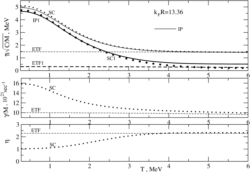
Figure 25: Collective vibration energy $\hbar\sqrt{C/M}$, reduced friction $\gamma/M$, and effective frictions $\eta=\gamma/2\sqrt{MC}$, determined at the same $k_{F}R$ value as in Fig. 24, versus the temperature $T$. top: The ETF curve (thin dashed) and the SC curve (dots) are determined respectively through the stiffness $C_{\rm{LD}}$ (IV.2.1) and inertia $M_{\rm ETF}$ (IV.2.2) for the first and through the SCM stiffness $C$ (IV.2.1) and the inertia $M$ (142) for the latter. The curves denoted by IP1 (thick solid line) and ETF1 (thick dashed line) are obtained in the IP and ETF approach, but including the Coulomb and surface corrections as explained in the main text, and SC1 (heavy squares) shows the corresponding SCM quantity; middle: ETF and SC curves show the reduced friction defined with the inertia $M_{\rm ETF}$ and the renormalized SCM inertia $M$ (142) respectively, with the friction $\gamma=\gamma_{\rm ETF}$ given by (IV.2.2); bottom: Effective friction $\eta=\gamma/2\sqrt{MC}$ obtained with a value of $J=30$ MeV in the ETF and SC approaches; all other parameters are the same as in Figs. 22 and 23.

Fig. 25 displays the temperature dependencies of the quadrupole collective-excitation energies, $\hbar\sqrt{C/M}$, reduced friction, $\gamma/M$, and effective friction, $\eta=\gamma/2\sqrt{CM}$ (all in the ${\rm F}$ mode), for the SC model versus their consistent ETF approximation MGFyaf2007 and IP results at $\epsilon_{0}\rightarrow+0$, except for obvious IP zeros of the quantities proportional to $\gamma$. All the quantities in Fig. 25 are rather slow functions of temperature $T$ at large enough values, $T\hbox{\kern 1.00006pt\lower 2.58334pt\hbox{$\sim$} \kern-11.19997pt\raise 2.58334pt\hbox{$>$} \kern 1.00006pt}T_{\rm cr}$, see (139). As expected, the temperature for disappearance of the shell effects in all these quantities is near the critical $T_{\rm cr}$ (139) as in Fig. 24 for the inertia, $\delta M$, and the free energy, $\delta{\cal F}$, as well as for the stiffness, $\delta C$, shell corrections (Fig. 22). For high temperatures, $~{}T\hbox{\kern 1.00006pt\lower 2.58334pt\hbox{$\sim$} \kern-11.19997pt\raise 2.58334pt\hbox{$>$} \kern 1.00006pt}T_{\rm cr}$, the SC practically coincides with its almost constant TF asymptotics. The significant shell effects are naturally manifested at temperatures $T$ smaller than $~{}T_{\rm cr}$.

As shown in the top panel of Fig. 25, the IP (thin solid) and SC (dots) quadrupole-vibration energy parameter, $\hbar\sqrt{C/M}$, is approximated well by the ETF curve (thin frequent dashed) at temperatures $T\hbox{\kern 1.00006pt\lower 2.58334pt\hbox{$\sim$} \kern-11.19997pt\raise 2.58334pt\hbox{$>$} \kern 1.00006pt}T_{\rm cr}$, where the shell effects are exponentially small. Such a parameter at finite temperature might be used in analysis of the fission experimental data gonfro ; hilgonros ; frgon . Again, a good agreement between IP and SC energies, $\hbar\sqrt{C/M}$, can be found for all temperatures. It is similar to the results obtained for the inertia (Fig. 23) because of the same renormalized stiffness $C$ used in both IP and SC calculations, and the only inertia $M$ is critical in this comparison. The significant shell enhancement in the collective vibration energies, $\hbar\sqrt{C/M}$, at smaller temperatures improves comparison with the experimental results for the quadrupole collective states in magic cold nuclei MGFyaf2007 . In the small temperature limit, these energies are strengthed because of the minimum of the inertia, $\delta M$, and the maximum of the stiffness, $\delta C$, associated both with the minimum of the free energy, $\delta{\cal F}$, shell correction for a magic particle number. A small decrease of the vibration energy maximum at low temperatures is related mainly to a negative Coulomb stiffness correction $C_{\rm LD}^{\rm coul}$ given explicitly in MGFyaf2007 [see the IP1 (thick solid) for its IP result, and the SC1 (full heavy rare squares) for the corresponding SC renormalization with the smooth ETF1 high-temperature asymptotics (thick rare dashed) in this part of Fig. 25, see also bormot ; bormot1 . The other surface ($A^{-1/3}$) corrections (included also in IP1, SC1 and ETF1) are much smaller because of a large particle number $A$. It should be noted, however, that the comparison of our SC results with the experimental data for magic nuclei, discussed in MGFyaf2007 for instance for ${\rm Pb^{208}}$, requires certainly more realistic calculations bormot ; hofbook ; khodsap ; berborbro . On a qualitative level, we may only point out here that our SC results become more close to the experimental data for magic nuclei mainly because of accounting for the shell effects.

As seen in the middle panel of Fig. 25 for higher temperatures, the ETF reduced friction, $\gamma/M\approx\gamma_{\rm ETF}/M_{\rm ETF}$, [(IV.2.2) and (IV.2.2)] is of order of the estimation MGFyaf2007 , which is basically comparable within the same order as its evaluation from the experimental fission data in hilgonros for the nearly spherical shapes of compound nuclei. More exact SC values are notably enhanced at smaller temperatures because of the shell effects. Note that the maximum of $\gamma/M$ at zero temperature can be explained by minima of the both free energy ${\cal F}$ and inertia $M$ (Fig. 24) because there is no friction shell corrections at $\epsilon_{0}=+0$, according to (IV.2.2). In this comparison we should take into account that the ETF approach is expected to be a good approximation for significantly heated systems for which one may disregard shell effects. We neglected also the nuclear equilibrium deformations which influence essentially on the reduced friction for fission processes frgon ; ivhofpashyam ; gonfro ; hilgonros . We should expect also the importance of residue interactions as the two-body viscosity in this comparison.

Rather a strong overdamped motion, $\eta>1$, at temperatures $T\hbox{\kern 1.00006pt\lower 2.58334pt\hbox{$\sim$} \kern-11.19997pt\raise 2.58334pt\hbox{$>$} \kern 1.00006pt}T_{\rm cr}$, where the ETF practically coincides with the SC approximation, is shown in the bottom panel of Fig. 25. As seen from comparison of the ETF versus the SC, the effective friction $\eta$ is decreasing monotonically to about one with decrease of temperature because of the shell effects. These calculations are also roughly in agreement with evaluations of the effective damping coefficient, $\eta$, found from the experimental data on fission hilgonros .

Thus, our results for the collective vibration energies at zero temperature, as well as the reduced, and the effective-friction coefficients for larger temperatures are qualitatively in reasonable agreement with the experimental data frgon ; gonfro ; hilgonros ; MGFyaf2007 . We suggested in this Section the modified SCM for calculations of the nuclear transport coefficients for a slow collective motion. The consistent ETF approach can be used for the smooth parts of transport coefficients in this SCM modified with the collective dynamics. We pointed out the importance of the renormalization (SCM) procedure for inertia as for the shell correction calculations of the nuclear free energy and stiffness. The shell structure components $\delta M$ for the inertia and $\delta C$ for the stiffness are significant at small temperatures. According to the POT, they disappear approximately with increasing temperature by an exponential law at about the same critical temperatures $2\div 3$ MeV as well as the free-energy shell corrections $\delta{\cal F}$. After the SCM renormalization of the quantum transport coefficients we obtained somewhat improved results toward experimental data for the quadrupole vibration excitation energy at small temperatures, and for the reduced friction and effective damping parameters at large temperatures; as compared to the hydrodynamical model. The quantum and semiclassical SCM calculations of the transport coefficients might be helpful for understanding and overcoming some difficulties within the linear response theory at the finite two-body dissipation related to a residue interaction.

IV.2.4 Smooth trajectory corrections

In this Section, we shall deal with nonlinear effects in the transport coefficients because of their quadratic expression (83) and (84) through the Green’s function (II.1). Therefore, the smooth semiclassical nonlocal corrections to the transport parameters [(93) and (94)] because of the classical trajectories with finite actions might yield the significant contributions, in addition to the wall formula and ETF inertia.

The famous wall formula (WF) describing the local one-body friction, suggested originally by Swiatecki and his collaborators wall , was re-derived in many works based on the semiclassical and quantum arguments (see koonran ; MGFyaf2007 ; GMFprc2007 , for instance). Important non-adiabatic nonlinear corrections were used in the microscopic collective classical and quantum dynamics blocki , in particular for calculations of the excitation energy and its time derivatives blocki ; BMYpr ; BMYijmpe2012 . Then, the peculiarities of the excitation energies for many periods of oscillations of the classical dynamics were discussed BMYpr ; BMYijmpe2012 for several multipole surface shapes (the order of Legendre polynomials). However, some problems in the analytical study of a multipolarity dependence of the smooth one-body friction and inertia should be still clarified within the EGA of the POT (Section II).

For slow (small-amplitude) vibrations around the spherical equilibrium shape of a nucleus described explicitly through the mean field in terms, e.g., of the cavity with sharp edges, one can use (81) of the linear response theory hofbook to relate the transport coefficients (IV.1.1) through the “intrinsic” (friction $\gamma(0)$, and inertia $M(0)$) ones to the one-body Green’s function $G({\bf r}_{1},{\bf r}_{2};\varepsilon)$ magvvhof . This relationship is especially useful for the semiclassical derivations of transport coefficients. We shall not show sometimes, within this Section, the argument “0” of these transport coefficients for simplicity of notations writing comments if necessary to avoid misunderstanding. The tilde above statistically averaged quantities will be disregarded too within this Section because only such smooth ones will be considered up to the end of this Section IVB4. Using also the spherical symmetry of the equilibrium shape and its expansion in Legendre polynomials $P_{n}$, one has koonran :

$$\gamma = \int_{0}^{\pi}\hbox{d}\psi\;\hbox{sin}\psi\;P_{n}\left(\hbox{cos}\psi\right)\;\Upsilon\left(\psi\right),$$

$$M = \int_{0}^{\pi}{\mbox{d}}\psi\;\hbox{sin}\psi\;P_{n}\left(\hbox{cos}\psi\right)\;B\left(\psi\right),$$ (152)

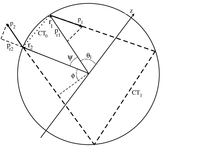
Figure 26: Classical trajectories CT₀ (dotted line) and CT₁ (dashed line) from initial point (${\bf r}_{1},{\bf p}_{1}$) in phase space to final point (${\bf r}_{2},{\bf p}_{2}$), as in Fig. 1, but at the boundary, with radial momentum components $p_{r1}$ and $p_{r2}$ respectively; $\psi$ is the angle between the ${\bf r}_{1}$ and ${\bf r}_{2}$ vectors, while $\theta_{1}$ (of ${\bf r}_{1}$) and $\phi$ are the angles in a spherical coordinate system with the polar axis $z$.

where $\psi=\theta_{2}-\theta_{1}$ is the polar angle between the two vectors ${\bf r}_{1}$ and ${\bf r}_{2}$. These vectors are arguments of the Green’s function $G({\bf r}_{1},{\bf r}_{2};\varepsilon)$ at the equilibrium surface in a major plane crossing any symmetry $z$ axis because of the spherical symmetry (Fig. 26). The kernels, $\Upsilon(\psi)$ and $B(\psi)$, for the integrals over $\psi$ are given by [(83) and (84)]

$$\Upsilon\left(\psi\right)=\frac{d_{s}\hbar^{5}R_{0}^{6}}{2m^{2}}\left(\frac{\partial^{2}{\mbox{\rm Im}}G}{\partial r_{1}\partial r_{2}}\right)^{2}_{r=R_{0},\varepsilon=\varepsilon_{F}},$$ (153)

$$B\left(\psi\right)=\frac{d_{s}\hbar^{6}R_{0}^{6}}{2m^{2}}$$

$$\times \int_{0}^{\varepsilon_{F}}\hbox{d}\varepsilon\left(\frac{\partial^{2}{\mbox{\rm Im}}G}{\partial r_{1}\partial r_{2}}\frac{\partial^{2}}{\partial\varepsilon^{2}}\frac{\partial^{2}{\mbox{\rm Re}}G}{\partial r_{1}\partial r_{2}}\right)_{r=R_{0}}.$$

For billiards, one writes $\varepsilon_{F}=p_{F}^{2}/2m$, where $p_{F}$ is the Fermi momentum. The effective mean field for motion of the particle at equilibrium is taken as the infinitely deep square-well potential depending on time $t$ through the multipole variations of a time-dependent surface radius $R(\theta,t)$ (IV.1.1), blocki keeping also the volume and the position of the center of mass conserved. The deformation parameter was traditionally introduced as $\alpha=q\sqrt{4\pi/5}$ to exclude a difference in constant between the Legendre polynomial description of the ES quadrupole and spheroidal shapes for small deformations blocki . In (153), $R_{0}$ is the radius of the equivalent sphere; and $\alpha(t)$ is a periodic function of time, $\alpha(t)=\alpha\hbox{cos}\left(\omega t\right)$, where $\alpha$ (without the argument $t$) is an amplitude. Thus, the rate of the excitation energy in time $t$ can be then written in terms of the consistent collective inertia $M$, and friction $\gamma$ [see (IV.1.1)] through the intrinsic ones $M(0)$ and $\gamma(0)$ given in (IV.2.4):

$$\hbox{d}E/\hbox{d}t=M\dot{\alpha}\ddot{\alpha}+\gamma\dot{\alpha}^{2}.$$ (154)

The friction $\gamma$ and inertia $M$ (intrinsic) coefficients [(IV.2.4) and (153)] can be found with the help of the semiclassical expansion of the Green’s function $G$ derived by Gutzwiller gutz ; strumag ; sclbook ; magvvhof for $k_{F}R\sim A^{1/3}\gg 1$ [$k_{F}$ is the wave number at the Fermi energy $\varepsilon_{F}$, see Section IVA2; and (II.1), (II.1), (II.1), and (4)].

Following koonran , according to the Green’s function expansion (II.1) over the CTs, one may split the transport coefficient kernels $\Upsilon(\psi)$ and $B(\psi)$ given by (153), both averaged over the phase space variables GMFprc2007 , into the two terms,

$$\Upsilon(\psi) = \Upsilon_{\rm wf}(\psi)+\Upsilon_{\rm corr}(\psi)\;,$$

$$B(\psi) = B_{\rm ETF}(\psi)+B_{\rm corr}(\psi)\;.$$ (155)

Here

$$\Upsilon_{\rm wf}(\psi)=\gamma_{\rm wf}\delta(\psi)/\hbox{sin}\psi\;,$$

$$\gamma_{\rm wf}\approx d_{s}\hbar(k_{F}R_{0})^{4}/(10\pi)$$ (156)

is the WF friction within the TF approach, according to MGFyaf2007 , and $~{}B_{\rm ETF}(\psi)=M_{\rm ETF}\delta(\psi)/\hbox{sin}\psi~{}$, where $M_{\rm ETF}$ presents the ETF (volume, surface and curvature) inertia terms [see (IV.2.2)]. These (local TF and nearly local ETF) terms are related to the short CT₀ component of the Green’s function trajectory expansion (II.1) after averaging over the phase space variables to remove their oscillations. Note that we have taken into account here the friction-dependent correction (148) to the intrinsic inertia $M(0)$ in (IV.2.2) for the smooth consistent collective inertia $M_{\rm ETF}$ MGFyaf2007 , i.e. ,

$$M\approx M_{\rm ETF}(0)+M_{\rm corr}^{(1)}+M_{\rm corr}^{(2)}\;,$$ (157)

where $M_{\rm ETF}(0)$ is the ETF component (IV.2.2), $M_{\rm corr}^{(1)}$ is the self-consistent correction (148) in the ETF inertia (IV.2.2), and $M_{\rm corr}^{(2)}$ the smooth nonlocal trajectory correction to the ETF inertia,

$$M_{\rm corr}^{(2)}=\int_{0}^{\pi}\hbox{d}\psi\;\hbox{sin}\psi\;P_{n}\left(\hbox{cos}\psi\right)\;B_{\rm corr}(\psi)\;,$$ (158)

and similarly, for the smooth trajectory-friction correction $\gamma_{\rm corr}^{(2)}$ in the sum $\gamma\approx\gamma_{\rm ETF}(0)+\gamma^{(2)}_{\rm corr}$. We neglected also a relatively small smooth nonlocal correction $\gamma_{\rm corr}^{(1)}$ [see (147)] to the friction $\gamma_{\rm ETF}(0)$ (IV.2.2) in calculations of the corresponding components of the inertia $M$ and friction $\gamma$ ($\gamma_{\rm corr}^{(1)}\ll\gamma_{\rm wf}$). The second terms $\Upsilon_{\rm corr}(\psi)$ and $B_{\rm corr}(\psi)$ in (IV.2.4) are the nonlocal corrections to the friction and inertia kernels, respectively,

$$\Upsilon_{\rm corr}(\psi) = \gamma_{\rm wf}\sum_{v,w}\frac{\hbox{sin}^{3}\phi\;\hbox{cos}\phi}{2v\hbox{sin}\psi}$$ (159)

$$\times \mathcal{R}_{\Upsilon}(\psi,v,w)\;,$$

$$B_{\rm corr}(\psi) = -M_{0}\sum_{v,w}\frac{\hbox{sin}^{3}\phi\;\hbox{cos}\phi|\hbox{sin}\phi|}{\hbox{sin}\psi}$$ (160)

$$\times \mathcal{R}_{B}(\psi,v,w),$$

where $M_{0}=d_{s}mR_{0}^{2}\;(k_{F}R_{0})^{3}/(16\pi^{2})$. The summations over $v$ and $w$ run over all CT$\neq$CT₀ from ${\bf r}_{1}$ to ${\bf r}_{2}$ in the spherical box (like T₁ shown in Fig. 26), in accordance with the Green’s function expansion (II.1). The number of sides $v\geq 2$ (intermediate vertexes plus one) and the winding number $w\leq$ [$v/2$] for clockwise and $w\geq-$[$v/2$] for anticlockwise motion specify the CT (the square brackets show the integer number of $v/2$). As shown in Fig. 26, $\phi$ is a half of the central angle for any chord of the equivalent sides of the trajectory, $\phi=\phi_{\rm PO}-\psi/(2v)$, $\phi_{\rm PO}=\pi w/v$, ($2v\phi+\psi=2\pi w$, see Fig. 26). In (159) and (160), we introduced also the modulation factors

$$\mathcal{R}_{\Upsilon}(\psi,v,w)\!=\!1\!-\!J_{0}\left[(\Delta S(\psi,v,w)/\hbar)^{1/2}\right],$$

$$\mathcal{R}_{B}(\psi,v,w)\!=\!1\!-\!J_{0}\left[(8\Delta S(\psi,v,w)/\hbar)^{1/2}\right]\;,$$ (161)

where $J_{0}(x)$ is the cylindrical Bessel function of zero order; and

$$\Delta S(\psi,v,w)=\pi p_{F}R_{0}\;\hbox{cos}\phi_{PO}\;\hbox{sin}\psi\;$$ (162)

is the action perturbation, $\Delta S_{\rm CT}$, depending on the relative angle $\psi$, and the $v,w$ integers which all specify the CT. Notice first that the calculation of the radial derivatives of the second terms (II.1) in the Green’s function expansion $G$ (equation (II.1)) are mainly (at leading order of $\hbar$) reduced to the derivatives of the action, $S_{\rm CT}=p\mathcal{L}_{\rm CT}$, where $\mathcal{L}_{\rm CT}=2R_{0}v\hbox{sin}\phi$ is the length of the CT in (153) for cavity-like potentials. These derivatives are the normal (radial) components of the particle momenta $p_{r1}$ and $p_{r2}$ at the spherical surface which are related to the initial ${\bf r}_{1}$ and the final ${\bf r}_{2}$ point, $p_{r\;1}=p_{r\;2}=p\;\hbox{sin}\phi$ (Fig. 26).

In contrast to the work koonran , we derive the expressions (159) for the friction and (160) for the inertia solving the symmetry breaking problem. Indeed, we have to integrate the kernels $\Upsilon(\psi)$ and $B(\psi)$ in (IV.2.4) over all $\psi$ from $0$ to $\pi$. However, in the limit $\psi\rightarrow 0$ a nonclose isolated trajectory of the type of T₁ (Fig. 26) turns into the degenerated one-parametric family of the closed periodic orbits. The parameter of each of these families is the angle of the rotation of a periodic orbit (PO) around the $z$ axis directed from the center of the spherical box to the vertex point ${\bf r}_{1}={\bf r}_{2}={\bf r}$ with the same action ($\phi=\phi_{\rm PO}$). The expression for the Green’s function amplitude ${\cal A}_{\rm CT}$ in (II.1) for the contribution of the PO family is in principle enhanced by the semiclassical factor $\hbar^{-1/2}$ as compared to that for the isolated trajectory (4) due to the one-parametric PO degeneracy strumag ; migdalrev (Section II). With $\psi$ decreasing to zero, one has a sharp increase of the Green’s function amplitudes within the angle of order of the wave length $1/k_{F}$ over the size $R_{0}$ of the Fermi system at $1/k_{F}R_{0}\ll 1$. Applying these expressions for the Green’s function amplitudes from strumag ; magvvhof to the smooth friction and inertia corrections (IV.2.4) at $\psi=0$, one in fact obtains zeros for the PO contributions because of the summations over all positive $w$ (for clockwise) and negative $w$ (for anticlockwise) motion with the odd summands in $w$. However, their analytical behavior is important for a continuous match of the transport coefficients with the asymptotic Gutzwiller ones related to the isolated trajectories T₁ at nonzero $\psi\gg 1/k_{F}R_{0}$.

The smooth transition between this asymptotics for the friction and inertia kernels, $\Upsilon(\psi)$ and $B_{\rm corr}(\psi)$ and the limit $\psi\rightarrow 0$ can be found by using the uniform approximation sclbook . This transition can be considered as a perturbation of the action, $\Delta S_{\rm CT}=\Delta S(\psi,v,w)$ (162), due to the symmetry breaking at $\psi=0$. Then, we transform a cycle variable, say $\varphi$ at $\psi=0$, into another cycle one $\widetilde{\varphi}=\widetilde{\varphi}(\varphi)$ (not necessary to be specified) with the increasing parameter $\psi$ such that for the phase integral $\Phi_{\rm CT}$ of the semiclassical Green’s function in (II.1) strumag ; sclbook , one finds by definition,

$$\Phi_{\rm CT}(\tilde{\varphi})\equiv\Phi_{\rm CT}(\varphi)$$ (163)

$$= \tilde{\Phi}^{0}_{\rm CT}+\sqrt{8\;\Delta S_{\rm CT}/\hbar}\;\hbox{cos}\left(\tilde{\varphi}\right)\;,$$

for the inertia calculations and without factor 8 in front of $\Delta S_{\rm CT}$ under the square root for the friction ones. The unknown constants $\widetilde{\Phi}^{0}_{\rm CT}$ and $\Delta S_{\rm CT}/\hbar$ can be found now from the two asymptotic solutions at the $\psi\rightarrow 0$ and $\psi\gg 1/k_{F}R_{0}$ limits for the friction $\Upsilon_{\rm corr}(\psi)$ and inertia $B_{\rm corr}(\psi)$ components of (IV.2.4). We emphasize that these transport coefficients are quadratic in $G$ rather than linear one for the level density calculations in the standard procedure for the uniform approximations sclbook . Therefore, in contrast to the standard transformation which is linear in the action perturbation $\Delta S_{\rm CT}$, see sclbook , called as the “pendulum transformation”, one finds a square root of $\Delta S_{\rm CT}$ in (163). Finally, one obtains the uniform approximation (159) and (160) for the smooth nonlocal friction and inertia corrections in terms of the modulation factor $\mathcal{R}(\psi,v,w)$ (IV.2.4). These results for $k_{F}R_{0}\rightarrow\infty$ ($\mathcal{R}(\psi,v,w)\rightarrow 1$) as functions of $\phi$ coincide formally with the smooth trajectory corrections found in koonran . By using a different method, one obtains the same results as presented in koonran if we ignore, nevertheless, the significant symmetry breaking for the transition from the PO family to the isolated CT contributions. This symmetry breaking leads to the divergences which can be removed for the friction calculations by the artificial procedure suggested in koonran . One finds the same reason also for the divergences of the inertia for which, however, this procedure does not help (for even $n$). Notice also that the definition of the angle itself $\phi$ is different from that of koonran . The action perturbation $\Delta S_{\rm CT}(\psi)$ (162) in units of $\hbar$ with a small $\psi$ measures the width in the variable $\psi$, $\psi\hbox{\kern 1.00006pt\lower 2.58334pt\hbox{$\sim$} \kern-11.19997pt\raise 2.58334pt\hbox{$<$} \kern 1.00006pt}\hbar/\Delta S_{\rm CT}\sim 1/\pi k_{F}R_{0}<<1$, for the uniform transition between the two abovementioned limits at a finite $k_{F}R_{0}$ , the contribution of the PO family, and the Gutzwiller limit for the isolated CT.

Our results (159) and (160) for $\Upsilon_{\rm corr}$ and $B_{\rm corr}$ associated with the smooth trajectory corrections at finite values $k_{F}R_{0}$ essentially differ from their asymptotics $k_{F}R_{0}\rightarrow\infty$ by the modulation factor $\mathcal{R}(\psi,v,w)$ defined in (IV.2.4) in terms of the Bessel function $J_{0}$, and therefore, from those of koonran . We obtained the finite $\psi$ dependence of the nonlocal friction- and inertia-correction kernels, $\Upsilon_{\rm corr}(\psi)$ (159) and $B_{\rm corr}(\psi)$ (160), respectively, due to smooth contributions of the T₁-like classical trajectories (Fig. 26). In order to see the convergence of summations over the trajectories $v$ and $w$ in $\Upsilon_{\rm corr}$ (159) [or $B_{\rm corr}$ in (160)] with our definition of $\phi$, one can subtract $\hbox{sin}^{3}\phi_{\rm PO}\hbox{cos}\phi_{\rm PO}$ from $\hbox{sin}^{3}\phi\hbox{cos}\phi$, and add the same one in the correction summand. The additional extra component of the friction $\Upsilon_{\rm corr}$ (or inertia $B_{\rm corr}$) is identically zero because of the symmetry of the summation over negative (anticlockwise) and positive (clockwise) winding numbers $w$ provided that the summand is an odd function of $w$, as mentioned above. Thus, the summation over positive and negative $w$ in (159) for the friction coefficient correction gives one more factor multiplier approximately $\propto 1/v$ at large $v$ ($\psi\leq\pi$, $|w|\leq[v/2]$). This leads to the fast convergence of sum over the trajectories specified by $v,w$ after the summation in $w$ as $1/v^{2}$. More slow convergence ($\propto 1/v$) over these trajectories occurs for the inertia coefficient correction (160). A slow convergence, $\sim 1/v$, takes nevertheless place because of oscillations in the numerator of the inertia summation for large $v$ (alternating series at large $v$) .

The smooth friction coefficients $\gamma$ (153) and (159) in units of $\gamma_{wf}$ show their essential difference from the w.f. for smaller multipolarities $n$, especially for the quadrupole friction (Table 3). With increasing $n$, they decrease toward one in agreement with the results of koonran , see last line taken from koonran . However, the friction coefficient $\gamma$ depends much on the finite $k_{F}R_{0}$ value. The limit $k_{F}R_{0}\rightarrow\infty$ shown in Table 3 can be compared with the results of koonran . As seen from Table 3, we found an essential difference of the friction coefficients for all multipolarities, especially for smaller even $n$, from those of koonran for $\gamma/\gamma_{\rm wf}$ which are independent of $k_{F}R_{0}$. But there is no dramatic difference between the smooth friction for the quadrupole and octupole dynamical surface distortions, in contrast to that found in koonran .

We present the smooth inertia ratios $M/M_{\rm irr}$ [see (157)] for several values of $k_{F}R_{0}$ in Table 4. The $k_{F}R_{0}$ dependence of these ratios appears mainly through the ETF values $M_{\rm ETF}/M_{\rm irr}$ (numbers shown in the brackets). Their self-consistent positive surface component [see $M_{\rm corr}^{(1)}$ (148) in (IV.2.2)] is dominating at smaller $k_{F}R_{0}$ and disappears at $k_{F}R_{0}\hbox{\kern 1.00006pt\lower 2.58334pt\hbox{$\sim$} \kern-11.19997pt\raise 2.58334pt\hbox{$>$} \kern 1.00006pt}10$ as the surface correction, proportional relatively to $A^{-1/3}$ with respect to the volume irrotational-flow inertia. The corrections $M_{\rm corr}^{(2)}/M_{\rm irr}$ are much less sensitive to the variations of $k_{F}R_{0}$ than for the friction $\gamma_{\rm corr}^{(2)}/\gamma_{\rm wf}$ (c.f. Tables 3 and 4). Note that our results for the inertias differ significantly from the ones obtained in koonran (last line of the Table 4). The quantities $M/M_{\rm irr}$ for even $n$ are finite, in contrast to the divergent results of koonran (even after the renormalization procedure suggested in koonran to avoid divergence). For the quadrupole vibrations, one finds the positive values of $M$ of the order of $M_{\rm irr}$ for smaller $k_{F}R_{0}\hbox{\kern 1.00006pt\lower 2.58334pt\hbox{$\sim$} \kern-11.19997pt\raise 2.58334pt\hbox{$<$} \kern 1.00006pt}10$ (160). The inertia $M$ for larger $k_{F}R_{0}$ are not shown because of almost the same smooth trajectory (nonlocal) correction $M_{\rm corr}^{(2)}$, and the ETF (nearly local) part $M_{\rm ETF}$ [$M_{\rm ETF}(0)$ and $M_{\rm corr}^{(1)}$ components] are unknown as we do not know what are the parameters, especially the isoscalar surface-energy constant $b_{\rm S}$ of the ETF ES MGFyaf2007 for so large particle numbers. In particular, by this reason, the values of the inertia $M/M_{\rm irr}$ in the limit $k_{F}R_{0}\rightarrow\infty$ should be improved. With increasing multipolarity $n$, one obtains much larger inertia $M$ as compared to its irrotational value $M_{\rm irr}$ bormot . For odd multipolarities one has significantly larger inertia, in contrast to much smaller values obtained in koonran , even after the renormalization procedure which is rather artificial for the inertia.

Concluding we have obtained the smooth nonlocal corrections from longer trajectories to the WF friction and ETF inertia coefficients within the EGA POT by using the uniform approximation for solving the symmetry breaking problem. The convergence of the friction corrections to the WF was found with increasing multipolarity of the surface distortions. The inertia parameters are larger than the irrotational flow value in the nuclear region of particle numbers.

IV.3 MAJOR-SHELL EFFECTS IN THE DISSIPATIVE
NUCLEAR DYNAMICS

As shown semiclassically in the previous Sections, many dynamical problems, in particular, in nuclear physics can be reduced to the collective motion of independent particles in a mean field with a relatively sharp time-dependent ES within the microscopic-macroscopic approaches myswann69 ; strut . In recent years it became apparent that the collective nuclear dynamics is very much related to the nature of the nucleonic motion. Behavior of the nucleonic dynamics is important in physical processes as fission and heavy ion collisions where a great amount of the collective energy is dissipated into a chaotic nucleonic motion. We have to mention here very intensive studies of the one-body dissipative phenomena described largely through the macroscopic wall formula for the excitation energy rate with taking into account the non-adiabatic nonlinear corrections (Section IVB4 and myswann69 ; wall ; blocki ; koonran ; GMFprc2007 ). For instance, it was extended to the microscopic collective classical and quantum dynamics. We like also to emphasize the significance of the transparent classical picture through the Poincaré sections of surfaces and Lyapunov exponents showing the order-chaos transitions, and quantum results for the average of the time-dependent excitation energy rate blocki . Then, the peculiarities of the excitation energies for many periods of the oscillations of the classical dynamics were discussed for the ES described by several Legendre polynomials BMYijmpe2012 . The statistics of the spacing between the neighboring levels and its relation to the shell effects depending on the specific properties of the s.p. spectra, as well as the multipolarity and deformation of the ES shapes were studied BMstatlevPRC2012 . Our main purpose in this Section is to look at the time-dependent derivatives of the excitation energies of the quantum gas of particles and focus to their correlations with the shell effects at slow and small-amplitude collective motion.

IV.3.1 Time-dependent energy rate

To study the shell effects in the friction coefficients, we start with the time-dependent s.p. Schrödinger equation for the wave function $\psi(t)$ blocki ,

$$i\hbar\partial\psi/\partial t=\hat{H}(t)\psi\;.$$ (164)

The Hamiltonian $\hat{H}(t)$ describes a gas of independent particles. For the deformed Woods-Saxon (WS) potential one has

$$V\left(r,\theta,t\right)=-\frac{V_{0}}{1+\hbox{exp}\left\{\left[r-R(\theta,t)\right]/a\right\}}\;,$$ (165)

depending on time $t$ through a time-dependent radius of the effective surface $R(\theta,t)$ wall ; blocki ; BMYpr

$$R(\theta,t) = \frac{R_{0}}{\Lambda(t)}\left[1+\alpha(t)\;\sqrt{\frac{4\pi}{5}}\;Y_{n0}\left(\theta\right)\;\right.$$ (166)

$$+ \left.\alpha_{1}(t)\sqrt{\frac{4\pi}{3}}\;Y_{10}\left(\theta\right)\right]\;.$$

Here, $\Lambda(t)$ is a normalization factor ensuring a volume conservation, $\alpha_{1}(t)$ stands for keeping a fixed position of the center of mass for odd multipolarities, and $R_{0}$ is the radius of the equivalent sphere, $Y_{n0}(\theta)=\sqrt{(2n+1)/4\pi}\;P_{n}\left(\hbox{cos}\theta\right)$. $P_{n}\left(\hbox{cos}\theta\right)$ is the Legendre polynomial, and $\alpha(t)$ a periodic function of time. For the collective multipole vibrations (166) near the spherical shape, one may write $\alpha(t)=\alpha\hbox{cos}\left(\omega t\right)$ where $\alpha$ is their amplitude [$\alpha(t)=q(t)(4\pi/5)^{1/2}$ where $q(t)$ is the deformation parameter as in Section IVB4].

Starting with oscillations from a maximum displacement of the $P_{n}$ deformation equal to $\alpha$, one can traditionally blocki introduce the adiabaticity parameter $\eta_{\rm ad}$ being the ratio of the biggest wall speed to the biggest speed of particles:

$$\eta_{\rm ad}=\alpha\omega/\Omega,\qquad\qquad\Omega=v_{F}/R_{0}\;,$$ (167)

where $\omega$ and $\Omega$ are the frequencies of the collective and particle motions with the Fermi velocity $v_{F}$. Note that a condition of smallness of the frequency $\omega$ with respect to $\Omega$ is used often in the nuclear collective dynamics, in particular, within the microscopic-macroscopic approaches myswann69 ; strut ; fuhi . Again, $\Omega$ determines the distance between the major shells strumag ; migdalrev ; sclbook , $\hbar\Omega\sim\varepsilon_{F}/A^{1/3}\approx 7-10$ MeV in heavy nuclei, with the Fermi energy $\varepsilon_{F}$ and the particle number $A$ in nucleus (Section II).

For small amplitude vibrations around the sphere, one can use an approximate expression for the rate of the excitation energy of the gas wall ,

$$\frac{dE}{dt}=m\rho\bar{v}\oint\dot{n}^{2}\hbox{d}S\;,$$ (168)

where $\rho$ is the particle density, $\bar{v}$ the mean particle speed, and $\dot{n}$ the normal speed of the surface element of the wall. The integral is taken over the entire surface.

Solutions to the dynamical equation (164) for the wave function $\psi(t)$, $\psi(t)=\sum_{i}C_{i}(t)\phi_{i}$, is taken as an expansion over the eigenfunctions $\phi_{i}$ of the static eigenvalue problem: $\hat{H}_{0}\phi_{i}=\varepsilon_{i}\phi_{i}$ , where $\hat{H}_{0}$ is a static Hamiltonian taken at the spherical shape. Thus, the problem is reduced to calculations of the time-dependent coefficients $C_{i}(t)$.

IV.3.2 Averaged energy rates and shell effects

The s.p. spectra are calculated for the quadrupole and octupole shapes of the WS potential (165) are presented in BMYijmpe2012 . For the solution of the eigenvalue problem, it is convenient to use the expansion over the well-known deformed axially-symmetric harmonic-oscillator basis blocki . To study the quantum-classical correspondence BMYpr we deal with the WS potential (165) having a sharp edge (diffuseness $a=0.1$ fm) and large depth ($V_{0}=200$ MeV), similarly to those of a classical motion of particles inside the container with the infinitely deep depth and sharp walls. The spectra are having the strong shell effects at small deformations near the spherical shape BMYijmpe2012 . The magnitudes of inhomogeneity of the s.p. levels near the Fermi energy, i.e. , the shell effects, become smaller at deformations $\alpha\gtrsim 0.1$ because of the symmetry breaking (Section II, strumag ; migdalrev ; sclbook ). However, the shell effects are not decreasing with deformations as the considered ES multipolarities have the same azimuthal symmetry which leads to a partial integrability of the Hamiltonian $\hat{H}_{0}$ having the deformed potential migdalrev .

Figs. 27 and 28 show the quadrupole $(P_{2})$ and octupole $(P_{3})$ averages of the time derivatives of the excitation energies, $\langle dE/dt\rangle$, for a slow collective motion, $\omega/\Omega=$ $0.2$, with a small amplitude, $\alpha\sim 0.1$, and corresponding shell-correction energies $\delta E$ as functions of the particle number parameter $N^{1/3}$, $N$ is the neutron number in nucleus. These averages are proportional to the one-body friction coefficient $\gamma$,

$$\langle dE/dt\rangle=\gamma\omega^{2}\alpha^{2}/2\;.$$ (169)

For the corresponding WF (168), derived within the TF approach, one finds

$$\langle dE/dt\rangle_{\rm wf} = \gamma_{\rm wf}\omega^{2}\alpha^{2}/2$$ (170)

$$= 9\varepsilon_{F}\eta_{\rm ad}\;\alpha\;\omega A/20\;.$$

The quantum numerical results for $\langle dE/dt\rangle$ are small as compared to those of the WF (170). However, as clearly seen from these Figures, especially in Fig.  28 for the octupole vibrations, one can observe rather strong correlations between the fluctuations of the time-dependent energy-rate average $\langle dE/dt\rangle$ depending on the particle number, $N^{1/3}$, and those of the shell-correction energies, $\delta E$, in good agreement with the shell effects in spectra near the spherical shape (Fig. 22). These correlations should be expected from the results of BMYijmpe2012 for the shell fluctuations of the level densities and energies, respectively. Note that for $\alpha\lesssim 0.1$, the positions of the minima and maxima of the shell correction energies, $\delta E$, become almost the same, at least for not too large particle numbers, though the amplitude of $\delta E$ as oscillating function of $N^{1/3}$ increases with decreasing deformation, c.f. the solid curve for $\alpha=0.1$ and dashed for $\alpha=0.05$ in the bottom panel of Fig. 28. For such a small $\alpha$, one should not expect significant differences between the friction coefficients for the quadrupole and octupole vibrations because the energy level structure becomes almost the same for all multipolarities at the small-amplitude collective motion. The excitation energy should be correlated to the shell structure of levels around the Fermi surface through an inhomogeneous distribution of the energy levels $\varepsilon_{i}$ near the Fermi surface $\varepsilon_{F}$, i.e. , the shell effects in the level density at the energy $\varepsilon\approx\varepsilon_{F}$.

Notice that the smooth semiclassical friction $\gamma/\gamma_{\rm wf}$ in the limit of the small amplitudes ($\alpha\rightarrow 0$) and frequencies ($\omega\rightarrow 0$) of vibrations of the spherical box is much larger (5 orders of the magnitude) than the averaged quantum values obtained in BMYijmpe2012 for slightly multipole deformed WS potential. Notice also that the results for friction coefficients depend on widths of the Gaussian averaging over the phase space variables GMFprc2007 . With decreasing widths one can find the situation with alternative contributions of the WF $\gamma_{\rm wf}$ and correction $\gamma_{\rm corr}$ in (IV.2.4). In this case, the WF might be not dominating and one has another explanation of the small-average quantum friction found in BMYijmpe2012 for the quadrupole and octupole vibrations.

The main period of the friction shell correction $\delta\gamma$ as function of the particle (neutron) number variable $N^{1/3}$ is of order of that of the energy shell correction $\delta E$ (see Section IVB). According to the POT strumag ; migdalrev ; sclbook it can be evaluated largely as $2\tilde{g}\hbar\Omega/3N^{2/3}\approx(N/A)^{1/3}/2\approx 0.4$ for large total particle numbers $A$ in the nucleus. (Here, $\hbar\Omega\approx 2\pi\hbar/t_{PO}\approx\varepsilon_{F}/A^{1/3}$, where $t_{\rm PO}$ is the period of motion of the particle along the shortest PO and $\widetilde{g}\approx 3N/4\varepsilon_{F}$ in the TF approximation for a smooth level density.) This is mainly in agreement with our numerical results presented in Figs. 27 and 28. The derivations of oscillating components of the friction coefficient (including the shell effects) due to other contributions of the CTs (also POs) within the POT will be presented elsewhere.

Thus, we found thus a fairly strong correlations between fluctuations of the excitation energies for a slow and small-amplitude vibration near the spherical shape and shell-correction energies. They are especially pronounced for the octupole case for which our dynamical calculations are far going to smaller deformations with a good accuracy. We obtained the smooth corrections related to longer trajectories to the wall formula within the POT and found convergence to the WF with increasing multipolarity of the surface distortions. The investigations of correlations between the shell effects and the dissipative character in the one-body friction coefficients within the semiclassical POT is under the way. It might be perspective to use the combined macroscopic-microscopic approaches and response function theory to clear up the results more systematically and analytically. Our quantum and semiclassical results can be helpful for understanding the one-body dissipation and inertia at slow and faster collective dynamics with different shapes like the ones met in nuclear fission and heavy-ion collisions.

V NUCLEAR COLLECTIVE ROTATIONS

This Section is devoted to one of the most remarkable and traditional subjects of nuclear physics. As mentioned in Introduction, within the cranking model (Section VA), one can use the extension of the Strutinsky SCM to the rotational problems by Pashkevich and Frauendorf fraupash ; mix . Within the semiclassical EGA POT approach, using also the response function theory and extended Gutzwiller expansion of the Green’s function over the classical trajectories as for other transport coefficients (Section IV), we significantly simplify the rotational many-body problem calculating the moments of inertia in terms of the ETF component (Section VB) and its shell correction (Section VC).

V.1 THE CRANKING MODEL

Within the cranking model, the nuclear collective rotation of a Fermi independent-particle system associated with a many-body Hamiltonian $\hat{\mbox{H}}$ can be described, to a good approximation eisgrei , in the restricted subspace of Slater determinants, by the eigenvalue problem for a s.p. Hamiltonian

$$\hat{H}^{\bm{\omega}}=\hat{H}+\hat{H}_{\rm CF}^{\bm{\omega}}\;,$$ (171)

usually referred to as the Routhian. For this Routhian, in the body-fixed rotating frame bormot ; mix ; fraupash , one has

$$\hat{H}^{\bm{\omega}}=\hat{H}+\hat{H}_{\rm CF}^{\bm{\omega}}=\hat{H}-\bm{\omega}\cdot\left(\hat{\bm{\ell}}+\hat{{\bf s}}\right),$$ (172)

where $\hat{H}_{\rm CF}^{\bm{\omega}}$ is the s.p. cranking field which is approximately equal (neglecting a smaller centrifugal term, $\propto\omega^{2}$) to the Coriolis interaction. The rotation frequency $\bm{\omega}$ of the body-fixed coordinate system (relative the laboratory system), and which is the Lagrange multiplier of our problem, is defined through the constraint on the nuclear angular momentum ${\bf I}$, evaluated through the quantum average $\langle\hat{\bm{\ell}}+\hat{{\bf s}}\rangle^{\bm{\omega}}={\bf I}$, of the total s.p. operator, $\hat{\bm{\ell}}+\hat{{\bf s}}$, where $\hat{\bm{\ell}}$ is the orbital angular momentum and $\hat{{\bf s}}$ is the spin of the quasiparticle, thus defining a function $\bm{\omega}=\bm{\omega}({\bf I})$. The quantum average of the total s.p. operator $\hat{\bm{\ell}}+\hat{{\bf s}}$ is obtained by evaluating expectation values of the many-body Routhian $\hat{\mbox{H}}_{\rm CF}^{\bm{\omega}}$ in the subspace of Slater determinants. For the specific case of a rotation around the $x$ axis ($\omega=\omega_{x}$) which is perpendicular to the symmetry $z$ axis of the axially-symmetric mean field $V$, one has (dismissing for simplicity spin (spin-isospin) variables),

$$\langle\hat{\ell}_{x}\rangle^{\omega} \equiv d_{s}\sum_{i}n_{i}^{\omega}$$ (173)

$$\times \int\hbox{d}{\bf r}\;\psi_{i}^{\omega}\;\left({\bf r}\right)\;\hat{\ell}_{x}\;\overline{\psi}_{i}^{\omega}\left({\bf r}\right)=I_{x}\;.$$

The spin (spin-isospin) degeneracy $d_{s}$ accounts for the symmetry of the mean-field potential $V({\bf r})$. The occupation numbers $n_{i}^{\omega}$ for the Fermi system of independent nucleons are given by

$$n_{i}^{\omega} \equiv n\left(\varepsilon_{i}^{\omega}\right)$$ (174)

$$= \{1+\hbox{exp}\left[(\varepsilon_{i}^{\omega}-\lambda^{\omega})/T\right]\}^{-1}\;.$$

In (173), $\psi_{i}^{\omega}({\bf r})$ are the eigenfunctions, and $\overline{\psi}_{i}^{\omega}({\bf r})$ their complex conjugate; $\varepsilon_{i}^{\omega}$ the eigenvalues of the Routhian $\hat{H}^{\omega}$ (172); $\lambda^{\omega}$ is the chemical potential. For relatively small frequencies $\omega$ and temperatures $T$, $\lambda^{\omega}$ is, in a good approximation equal to the Fermi energy, $\lambda^{\omega}\approx\varepsilon_{{}_{\!{\rm F}}}=\hbar^{2}k_{\rm F}^{2}/2m^{*}$, where $k_{{}_{\!{\rm F}}}$ is the Fermi momentum in units of $\hbar$ and $m^{*}$ is the effective mass. From (173), the rotation frequency $\omega$ can be specifically expressed in terms of a given angular momentum $I_{x}$ of the nucleus: $\omega=\omega\left(I_{x}\right)$. Within the same approach, one approximately has for the particle number

$$A = d_{s}\sum_{i}n_{i}^{\omega}\int\hbox{d}{\bf r}\;\psi_{i}^{\omega}({\bf r})\;\overline{\psi}_{i}^{\omega}({\bf r})$$ (175)

$$\approx d_{s}\int\hbox{d}\varepsilon\;n(\varepsilon)\;,$$

which determines the chemical potential $\lambda^{\omega}$ for a given number $A$ of nucleons. Since we introduce the continuous parameter $\omega$ and ignore the uncertainty relation between the angular momentum and the rotation angles of the body-fixed coordinate system, the cranking model is semiclassical in nature ringschuck ; GMBBps2015 . One may thus consider the collective MI $\Theta_{x}$, for a rotation around the $x$ axis (omitting, to simplify the notation, spin and isospin variables), as a response of the quantum average $\delta\langle\hat{\ell}_{x}\rangle^{\omega}$ (173), to the external cranking field $\hat{H}_{\rm CF}^{\omega}$ in (172). Similarly to the magnetic or isolated susceptibilities richter ; fraukolmagsan ; magvvhof ; MGFyaf2007 , one can write

$$\delta\langle\hat{\ell}_{x}\rangle^{\omega}=\Theta_{x}(\omega)\delta\omega\;,$$ (176)

where

$$\!\Theta_{x}(\omega)=\partial\langle\hat{\ell}_{x}\rangle^{\omega}/\partial\omega=\partial^{2}E(\omega)/\partial\omega^{2},\quad\;\;\;$$

$$\!\!\!E(\omega)=\langle\hat{H}\rangle^{\omega}\equiv d_{s}\sum_{i}n_{i}^{\omega}\!\int\hbox{d}{\bf r}\;\psi_{i}^{\omega}\left({\bf r}\right)\!\hat{H}\overline{\psi}_{i}^{\;\omega}\left({\bf r}\right)\;.$$ (177)

A parallel (alignment) rotation with respect to the symmetry $z$ axis mix ; kolmagstr ; dfcpuprc2004 has also been considered in mskbPRC2010 .

For a nuclear rotation around the $x$ axis, one can treat, as was shown in inglis ; belyaevzel ; valat ; bormot ; fraupash ; mix , the term $-\bm{\omega}\cdot\hat{\bm{\ell}}=-\omega\,\hat{\ell}_{x}$ as a perturbation. With the constraint (173) and the MI (V.1) treated in the second order perturbation theory, one obtains the well-known Inglis cranking formula,

$$\Theta_{x}=d_{s}\;\sum_{ij}^{\;\;\;\;\;\;\;\prime}\;\frac{(n_{i}-n_{j})\;\Big{|}\langle j|\hat{\ell}_{x}|i\rangle\Big{|}^{2}}{\varepsilon_{i}-\varepsilon_{j}}\;,$$ (178)

where $\langle j|\hat{\ell}_{x}|i\rangle$ is the matrix elements of the angular-momentum projection operator $\hat{\ell}_{x}$ given in the middle of (173) at $\omega=0$, $|i\rangle=\psi_{i}$ (the superscript prime means again the exclusion of all terms with $\varepsilon_{i}=\varepsilon_{j}$, as in Eq. (85)). Instead of carrying out the rather involved calculations presented above, one could, to obtain the yrast line energies $E(I_{x})$ for small enough temperatures $T$ and frequencies $\omega$, approximate the angular frequency by $\omega=I_{x}/\Theta_{x}$ and write the energy in the form

$$E(I_{x})=E(0)+\frac{I^{2}_{x}}{2\Theta_{x}}\;.$$ (179)

As usually done, the rotation term above needs to be quantized through $I^{2}_{x}\rightarrow I_{x}(I_{x}+1)$ in order to study rotation bands.

V.2 SELF-CONSISTENT ETF DESCRIPTION
OF NUCLEAR ROTATIONS

Following references bartelnp ; belyaev , a microscopic description of rotating nuclei was obtained in the Skyrme Hartree–Fock formalism, within the ETF approach up to order $\hbar^{2}$. With a variational space restricted to Slater determinant, the minimization of the expectation value of the nuclear Hamiltonian leads to the s.p. Routhian $\hat{H}^{\bm{\omega}}_{\rm q}$ (172) that is determined by a one-body potential $\hat{V}_{\rm q}({\bf r})$, a spin-orbit field $\hat{{\bf W}}_{\rm q}({\bf r})$, and an effective-mass form factor $f^{\rm eff}_{\rm q}({\bf r})=m/m^{*}_{\rm q}$ (see also brguehak ). In what follows and throughout this Section, and to simplify the notation, we shall omit the hat sign on quantum mechanical operators of local quantities within the semiclassical approximation. In the case when the time reversal symmetry is broken, the additional cranking field $\bm{\alpha}_{\rm q}({\bf r})$ and spin field form factors ${\bf S}_{\rm q}({\bf r})$ appear. Here, and throughout this Section, a subscript q refers to the nucleon isospin (q = n, p), not to be confused with the deformation parameter or wave number $q$ in other Sections of this review. All these fields can be written as functions of the local densities and their derivatives, such as the neutron or proton particle densities $\rho_{\rm q}({\bf r})$, the kinetic energy densities $\tau_{\rm q}({\bf r})$, the spin densities (also referred to as spin-orbit densities) ${\bf J}_{\rm q}({\bf r})$, the current densities ${\bf j}_{\rm q}({\bf r})$, and the spin-vector densities $\bm{\rho}_{\rm q}({\bf r})$.  Note that in the present subsection, $\tau_{\rm q}({\bf r})$ stands for the kinetic-energy density which should not be confused with the neutron skin variable in Section III and Appendix A. In principle, two additional densities appear, a spin-vector kinetic-energy density $\bm{\tau}_{\rm q}({\bf r})$ and a tensor coupling $J_{ij}({\bf r})$ between spin and gradient vectors, which have, however, been neglected since their contribution should be small, as suggested by BFH87 .

The cranking-field form factor $\bm{\alpha}_{\rm q}({\bf r})$ contains two contributions, one of them coming from the orbital part of the constraint, $-\bm{\omega}\cdot\bm{\ell}$, which has been shown in BV78 to correspond to the Inglis cranking formula inglis , while the other, the Thouless–Valatin self-consistency contribution TV62 has its origin in the self-consistent response of the mean field to the time-odd part of the density matrix generated by the cranking term of the Hamiltonian. The aim is now to find functional relations for the local densities $\tau_{\rm q}({\bf r})$, ${\bf J}_{\rm q}({\bf r})$, ${\bf j}_{\rm q}({\bf r})$ and $\bm{\rho}_{\rm q}({\bf r})$ in terms of the particle densities $\rho_{\rm q}({\bf r})$, in contrast to those given by Grammaticos and Voros GV79 in terms of the form factors $V_{\rm q}$, $f^{\rm eff}_{\rm q}$, ${\bf W}_{\rm q}$, $\bm{\alpha}_{\rm q}$ and ${\bf S}_{\rm q}$. Taking advantage of the fact that, at the leading TF order, the cranking field form factor is given by bartelnp

$$\bm{\alpha}^{({\rm TF})}_{\rm q}=f^{\rm eff}_{\rm q}\left({\bf r}\times\bm{\omega}\right)\;,$$ (180)

one simply obtains the rigid-body value for the Thomas–Fermi current density

$${\bf j}^{({\rm TF})}_{\rm q}=\displaystyle\frac{m}{\hbar}\left(\bm{\omega}\times{\bf r}\right)\,\rho_{\rm q}\;.$$ (181)

This result is not that trivial, since it is only through the effect of the Thouless–Valatin self-consistency terms that such a simple result is obtained. Notice also that (181) corresponds to a generalization to the case $f^{\rm eff}_{\rm q}\neq 1$ of a result already found by Bloch Bl54 .

Equation (181) can also be considered as an extension of the Landau quasiparticle (generalized TF) theory landau ; abrikha ; belyaev presented in Section III and applied now, (if particle collisions can be neglected in the kinetic equation (47)), to the mean-field case of rotating Fermi-liquid systems (cf. (181) with the current density as an average of the particle velocity, ${\bf p}_{\rm rot}/m=\bm{\omega}\times{\bf r}$, rotating with the frequency $\bm{\omega}$ belyaev ). In particular, the re-normalization of the cranking field form factor $\bm{\alpha}^{({\rm TF})}_{\rm q}=f_{\rm q}^{\rm eff}\bm{\alpha}_{\rm o}$ with

$$\bm{\alpha}_{\rm o}=\left({\bf r}\times\bm{\omega}\right)\;,$$ (182)

by (180) can be also explained as related to the corrections, $f_{\rm q}^{\rm eff}\neq 1$, obtained by Landau landau with using both the Galileo principle and the Thouless–Valatin self-consistency corrections to a particle mass $m$ due to the quasiparticles’ (self-consistent) interaction through a mean field. They lead in bartelnp to the self-consistent TF angular momentum of the quasiparticle $\bm{\ell}_{\rm q}=f_{\rm q}^{\rm eff}\bm{\ell}_{\rm o}$ with the classical angular momentum $\bm{\ell}_{\rm o}={\bf r}\times{\bf p}$ of the particle, so that $-\bm{\omega}\cdot\bm{\ell}_{\rm q}=\bm{\alpha}_{\rm q}\cdot{\bf p}$. This effect is similar to that for the kinetic energies of the quasiparticles, $\varepsilon_{\rm q}=p^{2}/(2m^{*}_{\rm q})=f_{\rm q}^{\rm eff}\varepsilon_{\rm o}$ where $\varepsilon_{\rm o}=p^{2}/(2m)$. With this transparent connection to the Landau quasiparticle theory, it is clear that there is no contradictions with the TF $\hbar\rightarrow 0$ limit (182) of the current densities in the FLDM, accounting for the TF particle densities. In (181), $\hbar$ appears formally due to a traditional use of the dimensionless units for the angular momenta in the quantum-mechanical picture to compare with experimental nuclear data. Another reason is related to a consistent treatment of the essentially quantum spin degrees of freedom, beyond the Landau quasiparticle approach to the description of Fermi liquids, which have no straight classical correspondence, in contrast to the orbital angular momentum $\bm{\ell}$. For already smooth quantities, the convergence in the TF limit ($\hbar\rightarrow 0$) can be realized after a statistical (macroscopic) averaging over many s.p. (or more generally, many-body) quantum states. This averaging removes the fluctuating (shell) effects which appear in the denominators of the exponents within the POT ( Section II). Finally, the spin paramagnetic effect can be considered within the ETF approach, through a macroscopic averaging, along with the orbital diamagnetic contribution. For instance, the spin-vector density does not have a straight classical analogue, such as the orbital angular momentum, and has to be considered as a quantity of leading order $\hbar$.

It is now important to notice bartelnp that in an ETF expression of order $\hbar^{2}$, it is sufficient to replace quantities, such as the cranking field form factor $\bm{\alpha}_{\rm q}$, by their ETF expressions. (after the statistical averaging mentioned above). In the same way, to obtain a semiclassical expression for the spin-vector densities $\bm{\rho}_{\rm q}$ that is correct up to order $\hbar$, only TF expressions are required. One thus obtains for $\bm{\rho}_{n}$ and $\bm{\rho}_{p}$ a system of linear equations that can be easily resolved bartelnp . One also notices from this system of equations that the spin-vector densities are proportional to the angular velocity $\omega$. Exploiting the well known analogy of the microscopic Routhian problem with electromagnetism, one may then define spin susceptibilities $\chi_{\rm q}$,

$$\bm{\rho}_{\rm q}=\hbar\,\chi_{\rm q}\,\bm{\omega}\;.$$ (183)

The key question now is to assess the sign of these susceptibilities and to decide whether or not the corresponding alignment is of a “Pauli paramagnetic” character. The study of bartelnp shows that this is the case, i.e., that the spin polarization is, indeed, of paramagnetic character, thus confirming the conclusions of the investigation performed by Dabrowski Da75 in a simple model of non-interacting nucleons.

Since the cranking field $\bm{\alpha}_{\rm q}$ is, appart from its contribution coming from the constraining field $\bm{\alpha}_{\rm o}$ (182) only determined by the current densities ${\bf j}_{\rm q}$ and the spin-vector densities $\bm{\rho}_{\rm q}$, one can then write down in a simple way bartelnp the contributions to the current densities ${\bf j}_{\rm q}$ going beyond the TF approach. The semiclassical corrections of order $\hbar^{2}$ can be split into contributions $(\delta{\bf j}_{\rm q})_{\ell}$ and $(\delta{\bf j}_{\rm q})_{s}$ coming respectively from the orbital motion and the spin degree of freedom. It is found bartelnp that the orbital correction $(\delta{\bf j}_{\rm q})_{\ell}$ corresponds to a surface-peaked counter-rotation with respect to the rigid-body current proportional to $\left(\bm{\omega}\times{\bf r}\right)$, thus recovering the Landau diamagnetism characteristic of a finite Fermi gas. With the expressions of the current densities ${\bf j}_{\rm q}$ and the spin-vector densities $\bm{\rho}_{\rm q}$ up to order $\hbar^{2}$, one can then write down the corresponding ETF expressions for the kinetic-energy density $\tau_{\rm q}({\bf r})$ and spin-orbit density ${\bf J}_{\rm q}({\bf r})$.

Taking the explicit ETF functional expressions up to order $\hbar^{2}$ of all the densities entering our problem, one is able to write down the energy of the nucleus in the laboratory frame as a functional of these local densities,

$$E=\int\hbox{d}{\bf r}\;\rho\;\mathcal{E}[\rho_{\rm q},\tau_{\rm q},{\bf J}_{\rm q},{\bf j}_{\rm q}\;,\bm{\rho}_{\rm q}],$$ (184)

where $\rho=\rho_{n}+\rho_{p}$. Upon some integration by parts, one finds that $\mathcal{E}$ can be written as a sum of the energy density per particle of the nonrotating system $\mathcal{E}(0)$ and its rotational part, in line of (179). Within the ETF approach, one has from (184)

$$E_{\rm ETF}=\int\hbox{d}{\bf r}\rho\mathcal{E}(0)+\frac{1}{2}\Theta_{\rm ETF}^{({\rm dyn})}\,\omega^{2}\;,$$ (185)

where $\Theta_{\rm ETF}^{({\rm dyn})}$ is the ETF dynamical moment of inertia for the nuclear rotation with a frequency $\bm{\omega}$. This MI is given in the form:

$$\Theta_{\rm ETF}^{({\rm dyn})}=\Theta_{\rm orb.}^{({\rm dyn})}+\Theta_{\rm spin}^{({\rm dyn})}=\!m\sum_{\rm q}\int\hbox{d}{\bf r}\left\{r_{\perp}^{2}\,\rho_{\rm q}\right.$$

$$\left.-\!\frac{f^{\rm eff}_{\rm q}\rho^{1/3}_{\rm q}}{(3\pi^{2})^{(2/3)}}+\left[\frac{\hbar^{2}}{2m}\!+\!W_{0}\left(\rho\!+\!\rho_{\rm q}\right)\right]\,\chi_{\rm q}\right\}\;,$$ (186)

where $r_{\perp}$ is the distance of a given point to the rotation axis. The Skyrme-force strength parameter of the spin-orbit interaction $W_{0}$ is defined in Section III3 brguehak .

One notices that the ETF term which comes from the orbital motion turns out to be the classical rigid-body (TF) MI. Semiclassical corrections of order $\hbar^{2}$ come from both the orbital motion ($\Theta_{\rm orb.}^{({\rm dyn})}$) and from the spin degrees of freedom ($\Theta_{\rm spin}^{({\rm dyn})}$). The contribution $\Theta_{\rm orb.}^{({\rm dyn})}$ is negative corresponding to a surface-peaked counter rotation in the rotating frame. Such a behavior is to be expected for a N-particle system bound by attractive short-range forces BJ76 . The spin contribution $\Theta_{\rm spin}^{({\rm dyn})}$ turns out to be of the paramagnetic type, thus leading to a positive contribution which corresponds to an alignment of the nuclear spins along the rotation axis. It can also be shown BBQ93 that the ETF kinematic moment of inertia,

$$\Theta_{\rm ETF}^{({\rm kin})}=\displaystyle\frac{\langle{\bm{\ell}}+{\bf s}\rangle^{\omega}}{\omega},$$ (187)

is identical to the ETF dynamical moment of inertia presented above.

It is now interesting to study the importance of the Thouless–Valatin self-consistency terms. This has accomplished by calculating the MI in the ETF approximation but omitting, this time, the Thouless–Valatin terms. One then finds bartelnp the following expressions for the dynamical MI, in what is simply the Inglis cranking (IC) limit

$$\Theta_{\rm IC}^{({\rm dyn})} = m\sum_{\rm q}\int\hbox{d}{\bf r}\left[\frac{\rho_{\rm q}}{\left(f^{\rm eff}_{\rm q}\right)^{2}}\right.$$ (188)

$$+ \left.\frac{mB_{3}}{\hbar^{2}}\rho_{\rm q}\rho_{\bar{\rm q}}\left(\frac{1}{f^{\rm eff}_{\rm q}}-\frac{1}{f^{\rm eff}_{\bar{\rm q}}}\right)^{\!\!2}\right]r_{\perp}^{2},$$

where $\bar{\rm q}$ is the other charge state ($\bar{\rm q}\!\!=\!\!p$ when $\rm q\!\!=\!\!n$ and vice-versa) and $B_{3}$ is defined through the Skyrme force parameters $t_{1},t_{2},x_{1}$ and $x_{2}$ (see bartelnp ). Apart from the corrective term in $\rho_{\rm q}\,\rho_{\bar{\rm q}}$, one notices that the first term in the expression above, which is the leading term, yields, at least for a standard HF-Skyrme force where $f^{\rm eff}_{\rm q}\geq 1$, a smaller MI than the corresponding term in (V.2) containing the Thouless–Valatin corrections. It is also worth noting that in this approximate case, the kinematic MI is given by

$$\Theta_{\rm IC}^{({\rm kin})}=m\sum_{\rm q}\int\hbox{d}{\bf r}\;\frac{\rho_{\rm q}}{f^{\rm eff}_{\rm q}}\;r_{\perp}^{2}\;,$$ (189)

which turns out to be quite different from the above given dynamical MI, (188), obtained in the same limit (ETF limit, omitting the Thouless–Valatin self-consistency terms).

To investigate the importance of the different contributions to the total moment of inertia, self-consistent ETF calculations up to order $\hbar^{4}$ have been performed bartelpl for 31 nonrotating nuclei, imposing a spherical symmetry, and using the SkM^∗ Skyrme effective nucleon-nucleon interaction BQB82 . Such calculations yield variational semiclassical density profiles for neutrons and protons brguehak which are then used to calculate the above given moments of inertia. The nuclei included in this study are ¹⁶O, ⁵⁶Ni, ⁹⁰Zr, ¹⁴⁰Ce, ²⁴⁰Pu and three isotopic chains for Ca ($A\!=\!36-50$), Sn ($A\!=\!100-132$) and Pb ($A\!=\!186-216$). The results of these calculations are displayed in Figure 29 taken from bartelnp .

One immediately notices the absence of any significant isovector dependence. The good reproduction of the total ETF moment of inertia obtained by the TF (rigid-body) value is also quite striking. One finds that the semiclassical orbital and spin corrections are in fact not small individually but cancel each other to a large extent. To illustrate this fact the ETF moments obtained by omitting only the spin contribution are also shown on the Figure. One thus obtains a reduction of the Thomas–Fermi result that is about 6% in ²⁴⁰Pu but as large as 43% in ¹⁶O.

The Inglis cranking approach performed at the TF level underestimates the kinematic moment of inertia by as much as 25%, and the dynamical MI by about 50% in heavy nuclei, demonstrating in this way the importance of the Thouless–Valatin self-consistency terms.

In bartelnp , a crude estimate of the semiclassical corrections due to orbital and spin degrees of freedom has been made by considering the nucleus as a piece of symmetric nuclear matter (no isovector dependence as already indicated by the self-consistent results shown in Fig. 29 above). It turns out that these semiclassical corrections have an identical $A$ dependence ($A^{-2/3}$ relative to the leading order TF, i.e. , the classical rigid-body term)

$$\Theta_{\rm ETF}=\Theta^{(\rm RB)}_{\rm TF}\left[1+\left(\eta_{\ell}+\eta_{s}\right)A^{-2/3}\right]\;.$$ (190)

A fit of the parameters $\eta_{\ell}$ and $\eta_{s}$ to the numerical results displayed in Fig. 29 yields $\eta_{\ell}=-1.94$ and $\eta_{s}=2.63$ giving a total (orbital + spin) corrective term of $0.69\,A^{-2/3}$. For a typical rare-earth nucleus (A = 170) all this would correspond to a total corrective term equal to 2.2% of the classical rigid-body value, $\Theta^{(\rm RB)}_{\rm TF}$, resulting from a -6.3% correction for the orbital motion and a 8.5% correction for the spin degree of freedom.

Whereas in the calculations that lead to Fig. 29 above, spherical symmetry was imposed, fully variational calculations have been performed in bartelpl , imposing however the nuclear shapes to be of spheroidal form. In this way, the nuclear rotation clearly impacts on the specific form of the matter densities $\rho_{n}$ and $\rho_{p}$ which, in turn, in the framework of the ETF approach determine all the other local densities, as explained above.

Trying to keep contact to usual shape parametrisation with the standard quadrupole parameters $\beta$ and $\gamma$, these are chosen in such a way as to yield the same semi-axis lengths of the quadrupole drop as those obtained for the spheroids. As a result, Figure 30 shows the evolution of the equilibrium solutions (the ones that minimize the energy for given angular momentum) as a function of the nuclear spin I. One clearly observes that at low values of the angular momentum (I in the range between 0 and 50 $\hbar$) the nuclear drop takes on an oblate shape, corresponding to increasing values of the quadrupole deformation parameter $\beta$ with increasing I values, but keeping the non-axiality parameter fixed at $\gamma=60^{\circ}$. For larger values of the total angular momentum (I beyond 55 $\hbar$), one observes a transition into triaxial shapes, where the nucleus evolves rapidly to more and more elongated shapes. For even higher values of I (I beyond 70 $\hbar$) the nucleus approaches the fission instability. These results are in excellent qualitative agreement with those obtained by Cohen, Plasil and Swiatecki CPS74 in a rotating LDM (see matmatnak2010_12 ; hinsatnak2010_11 for a more microscopic description of the transitions between oblate and prolate shapes in nuclear rotational bands).

It is amusing to observe here a backbending phenomena at the semiclassical level when one is plotting, as usual, the MI $\Theta_{\rm ETF}$ versus the rotational angular momentum, as displayed in Fig. 31. One should, however, insist on the fact that this backbending has strictly nothing to do with the breaking of a Cooper pair. The rapid increase of the moment of inertia at about I$\,=60\hbar$ with a practically constant (or even slightly decreasing) rotational frequency $\omega$ comes simply from the fact that at such a value of I (between I $\approx$ 60 and I $\approx$ 70) the nucleus elongates substantially increasing in this way its deformation and at the same time its MI.

It is therefore interesting to notice that the semiclassical ETF approach leads to a moment of inertia that is very well approximated by its TF, i.e., the classical rigid-body value. Thouless–Valatin terms which arise from the self-consistent response of the mean field to the time-odd part of the density matrix generated by the cranking piece of the Hamiltonian are naturally taken care of in this approach. Semiclassical corrections of order $\hbar^{2}$ coming from the orbital motion and the spin degree of freedom are not small individually, but compensate each other to a large extent.

One has, however, to keep in mind that shell and pairing effects, that go beyond the ETF approach, are not included in this description. These effects are not only both present, but influence each other to a large extent, especially for the collective high-spin rotations of strongly deformed nuclei belyaevhighspin ; pomorbartelPRC2011 ; sfraurev .

V.3 SHELL-STRUCTURE MOMENT OF INERTIA

We apply the EGA POT (Section II) for the derivation of the MI through the rigid-body MI (with the shell corrections) in the NLA (Section IVA) related to the collective statistically equilibrium rotation with a given frequency $\omega$ mskbPRC2010 . For simplicity, we shall discard the spin and isospin degrees of freedom, in particular, the spin-orbit and asymmetry interaction. Notice also that from the results presented in Figs. 29 and 31 (with the help of Fig. 30), one may conclude that the main contribution to the moment of inertia of the strongly deformed heavy nuclei can be found within the ETF approach to the rotational problems as a smooth rigid-body MI. However, sometimes the MI shell corrections play the dominating role as traps in the yrast line for the deformed nuclei at high spins, like in ⁶⁰Dy strutdy152 , recall also the asymmetry of nuclear fission fragments because of the shell effects.

V.3.1 Green’s function trajectory expansion for the MI

For the derivations of shell effects strut within the POT sclbook ; gutz ; strumag ; bt76 ; creagh ; migdalrev ; MKApanSOL1 , it turns out to be helpful to use the coordinate representation of the MI through the Green’s functions $G\left({\bf r}_{1},{\bf r}_{2};\varepsilon\right)$ as for the other transport coefficients (Section IV) mskbg ; mskbPRC2010 ; magvvhof ; MGFyaf2007 ; GMSnpae2007 . In the coordinate representation, the MI $\Theta_{x}$ as a susceptibility (V.1) [or (176)] which is similar to the response function (81) for the collective vibrations, can be expressed in terms of the s.p. Green’s function $G$ by using its spectral representation (82) through the Inglis formula (178),

$$\Theta_{x}(\omega)=\frac{d_{s}}{\pi}\int^{\infty}_{0}{\rm d}\varepsilon\;n({\varepsilon})$$ (191)

$$\times {\mbox{\rm Re}}\int{\rm d}{\bf r}_{1}\int{\rm d}{\bf r}_{2}\;\ell_{x}({\bf r}_{1})\;\ell_{x}({\bf r}_{2})$$

$$\times\left[G\left({\bf r}_{1},{\bf r}_{2};\varepsilon-\hbar\omega\right)+\overline{G}\left({\bf r}_{1},{\bf r}_{2};\varepsilon+\hbar\omega\right)\right]$$

$$\times{\mbox{\rm Im}}\left[G\left({\bf r}_{1},{\bf r}_{2};\varepsilon\right)\right]\;.$$

The angular momentum operator $\ell_{x}$ in (191) takes a similar role of the s.p. operator named $\hat{F}$ (or $\hat{Q}$) in Section IV magvvhof ; GMFprc2007 ; MGFyaf2007 ; belyaev . For the adiabatic rotations one can neglect here the $\omega$-dependence,

$$\Theta_{x} = \frac{2d_{s}}{\pi}\int^{\infty}_{0}{\rm d}\varepsilon\;n({\varepsilon})$$ (192)

$$\times \int{\rm d}{\bf r}_{1}\int{\rm d}{\bf r}_{2}\;\ell_{x}({\bf r}_{1})\;\ell_{x}({\bf r}_{2})\;$$

$$\times {\mbox{\rm Re}}\left[G\left({\bf r}_{1},{\bf r}_{2};\varepsilon\right)\right]\;{\mbox{\rm Im}}\left[G\left({\bf r}_{1},{\bf r}_{2};\varepsilon\right)\right]\;.$$

This representation is useful within the semiclassical POT, weakening the criterium of the quantum perturbation approximation: The maximal rotational-excitation energy $\hbar\omega$ for which the approximation is valid becomes then significantly larger than the nearest neighbor s.p.-level spacing around the Fermi surface $\varepsilon_{F}$, but still somewhat smaller than the energy distance between major shells $\hbar\Omega$ ($\hbar\Omega\!\approx\!\varepsilon_{F}/A^{1/3}$) as shown by Migdal Migdal75 . This is in contrast to the cranking formula (178) derived with the help of the quantum perturbation criterion of smallness of the excitation energies with respect to this s.p. level spacing. The latter restriction appears probably because of using the spectral representation of the Green’s function $G$ in (191) and (192). Therefore, one can assume that this restriction is weakened through the coordinate representation of $G$, valid even for a quasi-continuous spectra of the semiclassical approximation.

V.3.2 Semiclassical Green’s function and particle density

For the s.p. Green’s function $G\left({\bf r}_{1},{\bf r}_{2};\varepsilon\right)$ in (191) and (192), we shall use the semiclassical Gutzwiller trajectory expansion (II.1), (II.1) and (4) as in Section IV gutz . The sum runs over the CT with particle energy $\varepsilon$ from a point ${\bf r}_{1}$ to a point ${\bf r}_{2}$ (see Fig. 1). There are several reasons leading to oscillations of the MI obtained from (192), some local (${\bf r}_{2}$ is close to ${\bf r}_{1}$) and some nonlocal (they are different), where the local PO part is related to the shell effects, whereas nonlocal (non-PO) contributions could have their origin in reflections of the particle from the boundary. The NLA ($|{\bf s}_{12}|\!=\!|{\bf r}_{2}\!-\!{\bf r}_{1}|\!\ll\!R$) is valid after a statistical averaging over many microscopic quantum states. Then, the maximal possible value of the parameter, which is the product of the two dimensionless quantities $\;\omega/\Omega$ and $\;S/\hbar$, used in dfcpuprc2004 as a small parameter of the perturbation approach of Creagh to the classical dynamics sclbook , in our EGA can be somewhat larger. This implies that $(\omega/\Omega)\;(S/\hbar)\hbox{\kern 1.00006pt\lower 2.58334pt\hbox{$\sim$} \kern-11.19997pt\raise 2.58334pt\hbox{$>$} \kern 1.00006pt}1$, under the usual semiclassical condition $S/\hbar\sim k_{F}R\sim A^{1/3}\gg 1$; where $k_{F}=p_{F}/\hbar$ is the Fermi momentum in $\hbar$ units, and $R$ the mean nuclear radius. According to (II.1), one can split also the Green’s function $G({\bf r}_{1},{\bf r}_{2};\varepsilon)$ into a contribution $G_{{\rm CT}_{0}}$ (II.1) coming from the direct path between the two points, ${\bf r}_{1}$ and ${\bf r}_{2}$, and a contribution $G_{{\rm CT}_{1}}$ that contains the contributions from all other trajectories involving reflections (II.1) (Fig. 1). For the component $G_{{\rm CT}_{0}}$ related to the trajectory CT₀ for which the action $S_{{\rm CT}_{0}}$ disappears in the limit ${\bf r}_{2}\to{\bf r}_{1}$, one finds again (II.1) with using ${\bf s}={\bf s}_{1,2}$, particle momentum $\,\,p({\bf r})\!=\!\sqrt{2m[\varepsilon-V({\bf r})]\,}$, and potential $V({\bf r})$, where $\;{\bf r}=({\bf r}_{1}+{\bf r}_{2})/2$. According to (192), for a semiclassical statistical-equilibrium rotation with constant frequency $\omega$, one approximately obtains mskbPRC2010 ; belyaev

$$\Theta\approx\Theta_{\rm GRB} = m\int\hbox{d}{\bf r}\;r_{\perp}^{2}\,\rho_{\rm scl}({\bf r})$$ (193)

$$= \Theta_{\rm ETF}+\delta\Theta_{\rm scl}\;,$$

where $\Theta_{\rm GRB}=\Theta_{\rm ETF}^{\rm GRB}+\delta\Theta_{\rm scl}^{\rm GRB}$ is the generalized rigid-body (GRB) MI with (Section VB and bartelnp ; belyaev )

$$\Theta_{\rm ETF}\approx\Theta_{\rm ETF}^{\rm GRB}=m\int{\rm d}{\bf r}\;r_{\perp}^{2}\,\rho_{ETF}\left({\bf r}\right)\;,$$ (194)

and $\delta\Theta_{\rm scl}$ its shell correction mskbPRC2010 ; belyaev ,

$$\delta\Theta_{\rm scl}\approx\delta\Theta_{\rm scl}^{\rm GRB}=m\int{\rm d}{\bf r}\;r_{\perp}^{2}\,\delta\rho_{\rm scl}({\bf r})$$ (195)

with $r_{\perp}^{2}=y^{2}+z^{2}$. Such a splitting (193) is associated with that of the spatial particle density $\rho({\bf r})$,

$$\rho({\bf r})\!=\!-\frac{1}{\pi}{\mbox{\rm Im}}\int{\rm d}\varepsilon n\left(\varepsilon\right)\!\left[G\left({\bf r}_{1},{\bf r}_{2};\varepsilon\right)\right]_{{\bf r}_{1}={\bf r}_{2}={\bf r}}.$$ (196)

Substituting (II.1) into (196), one obtains $\rho({\bf r})$ in terms of its ETF particle density $\rho_{\rm ETF}$ and its shell correction $\delta\rho_{\rm scl}({\bf r})$,

$$\rho_{\rm scl}\left({\bf r}\right)=\rho_{\rm ETF}+\delta\rho_{\rm scl}({\bf r})\;,$$ (197)

where

$$\rho_{\rm ETF}\left({\bf r}\right) = -\frac{1}{\pi}\,{\mbox{\rm Im}}\int{\rm d}\varepsilon\widetilde{n}\left(\varepsilon\right)$$ (198)

$$\times \left[G_{{\rm CT}_{0}}\left({\bf r}_{1},{\bf r}_{2};\varepsilon\right)\right]_{{\bf r}_{1}={\bf r}_{2}={\bf r}}$$

and

$$\delta\rho_{\rm scl}\left({\bf r}\right) = -\frac{1}{\pi}{\mbox{\rm Im}}\int\hbox{d}\varepsilon\delta n\left(\varepsilon\right)$$ (199)

$$\times \left[G_{{\rm CT}_{1}}\left({\bf r}_{1},{\bf r}_{2};\varepsilon\right)\right]_{{\bf r}_{1}={\bf r}_{2}={\bf r}}\;.$$

The standard decomposition of the occupation numbers

$$n=\widetilde{n}+\delta n$$ (200)

into the smooth and fluctuating parts is used as usually in the SCM fuhi . The crossing terms coming from the substitution of (200) and (II.1) into (196) almost do not contribute after the phase space integration by the SPM.

V.3.3 MI phase space trace formulas

Substituting (196) with (II.1) into (193), for the total semiclassical MI $\Theta_{x}$, one obtains the phase-space trace formula GMBBps2015 ; GMBBprc2016 :

$$\Theta_{\rm scl} \approx d_{s}\,m\!\int\!\hbox{d}\varepsilon\;\varepsilon\;n(\varepsilon)$$ (201)

$$\times \int\frac{{\rm d}{\bf r}_{2}{\rm d}{\bf p}_{1}}{(2\pi\hbar)^{3}}\;\frac{r_{2\perp}^{2}}{\varepsilon}\,g_{\rm scl}({\bf r}_{2},{\bf p}_{1};\varepsilon)\;$$

$$= \Theta_{\rm ETF}+\delta\Theta_{\rm scl}\;,$$

where

$$g_{\rm scl}({\bf r}_{2},{\bf p}_{1};\varepsilon)=\frac{\partial f({\bf r},{\bf p})}{\partial\varepsilon}$$ (202)

$$= G_{\rm scl}({\bf r}_{2},{\bf p}_{1};\varepsilon)\;\hbox{exp}\left[i\,{\bf p}_{1}\left({\bf r}_{1}\!-\!{\bf r}_{2}\right)/\hbar\right]\;.$$

The usual Wigner distribution function $f({\bf r},{\bf p})$ in the phase space ${\bf r},{\bf p}$, and now $r_{2\perp}^{2}=y_{2}^{2}+z_{2}^{2}$, were introduced (to simplify the notations the subscript 2 in $r_{2\perp}^{2}$ will be omitted in the following). Here $G_{\rm scl}({\bf r}_{2},{\bf p}_{1};\varepsilon)$ is a semiclassical Green’s function in the mixed phase-space representation obtained by the Fourier transformation of $G_{\rm scl}({\bf r}_{1},{\bf r}_{2};\varepsilon)$ (II.1),

$$\!G_{\rm scl}\!({\bf r}_{2},{\bf p}_{1};\varepsilon)\!=\!{\mbox{\rm Re}}\!\sum_{\rm CT}\!\Big{|}\!J_{\rm CT}\!\left({\bf p}_{1\perp},{\bf p}_{2\perp}\!\right)\!\Big{|}^{1/2}\!\delta\left[\varepsilon\!-\!H({\bf r}_{2},{\bf p}_{2})\right]\!\!$$

$$\times\hbox{exp}\!\left[\frac{i}{\hbar}S_{\rm CT}\left({\bf r}_{1},{\bf r}_{2};\varepsilon\right)\!-\!\frac{i\pi}{2}\mu_{\rm CT}\right],$$ (203)

where $J_{\rm CT}\left({\bf p}_{1\perp},{\bf p}_{2\perp}\right)$ is the Jacobian for the transformation from the component ${\bf p}_{1\perp}$ of the momentum ${\bf p}_{1}$ that is perpendicular to the reference CT to the perpendicular component ${\bf p}_{2\perp}$ of the momentum ${\bf p}_{2}$. We formally inserted the additional integral over ${\bf r}_{1}$ with $\delta({\bf r}_{2}-{\bf r}_{1})$ into the middle of (193) and transformed the spatial coordinates ${\bf r}_{1}$ and ${\bf r}_{2}$ to the phase space variables ${\bf r}_{2}$ and ${\bf p}_{1}$ MAFptp2006 ; belyaev . Using then the Fourier transformation of this $\delta$ function of the coordinate difference ${\bf r}_{2}-{\bf r}_{1}$ to a new momentum ${\tilde{\bf p}}$ and integrating, by the stationary phase method, the MI in such a phase space representation over the component of ${\tilde{\bf p}}$, perpendicular to the classical trajectories, one arrives at (201) MKApanSOL1 . Note that under the perfect local approach of the NLA (${\bf r}_{1}\rightarrow{\bf r}_{2}\rightarrow{\bf r})$ and ${\bf p}_{1}\rightarrow{\bf p}_{2}\rightarrow{\bf p}$ the ETF CT₀ component (II.1) of the Green’s function (II.1) is related to an energy density of the TF distribution function (202)

$$g_{\rm scl}({\bf r},{\bf p};\varepsilon)\rightarrow g_{\rm TF}({\bf r},{\bf p};\varepsilon)=\delta(\varepsilon-H({\bf r},{\bf p})).$$ (204)

V.3.4 ETF distribution function density

As shown in Appendix C, the ETF distribution density component, $g_{\rm ETF}({\bf r},{\bf p};\varepsilon)$, can be derived within the ETF approach by using the inverse Laplace transformation (C),

$$g_{\rm ETF}({\bf r},{\bf p};\varepsilon)=g_{\rm TF}+g_{\rm S}({\bf r},{\bf p};\varepsilon)\;,$$ (205)

where $g_{\rm TF}$ is given by (204). Taking also into account the same phase-space integration, one can simplify more this expression excluding formally the terms which do not contribute because of the integral over momentum ${\bf p}$. For the ETF surface correction $g_{\rm S}$, one obtains

$$g_{\rm S}({\bf r},{\bf p};\varepsilon)=\hbar^{2}\left\{\left(-\frac{\nabla^{2}V}{4m}\right)\right.$$ (206)

$$\times \left.\frac{\partial^{2}\delta\left(\varepsilon-H({\bf r},{\bf p})\right)}{\partial\varepsilon^{2}}\right.$$

$$+ \left.\left[\frac{\left(\nabla V\right)^{2}}{6m}+\frac{p^{2}\nabla^{2}V}{18m^{2}}\right]\;\frac{\partial^{3}\delta\left(\varepsilon-H({\bf r},{\bf p})\right)}{\partial\varepsilon^{3}}\;\right.$$

$$- \left.\frac{p^{2}\left(\nabla V\right)^{2}}{24m^{2}}\;\frac{\partial^{4}\delta\left(\varepsilon-H({\bf r},{\bf p})\right)}{\partial\varepsilon^{4}}\right\}\;.$$

The gradients of the potential, $(\nabla V)^{2}$ and $\nabla^{2}V$, can be expressed in terms of the those of the TF particle density within the same $\hbar^{2}$ precision, ,

$$\rho_{\rm TF}=d_{s}\frac{p_{\lambda}^{3}({\bf r})}{6\pi^{2}\hbar^{3}}\;,$$ (207)

where

$$p_{\lambda}({\bf r})=\sqrt{2m\left[\lambda-V({\bf r})\right]}\;.$$ (208)

Differentiating (207) and solving the obtained linear system of equations with respect to the potential gradient terms, one results in (B.40) and (B.41). These expressions are more convenient to use in a more general case including billiard systems as spheroidal cavity.

V.3.5 ETF and shell structure energies

Equation (201) strongly resemblances (except for the additional factor $mr_{\perp}^{2}/\varepsilon$) with the expression for the semiclassical s.p. energy

$$E_{\rm scl} = d_{s}\int\hbox{d}\varepsilon\;\varepsilon\;n(\varepsilon)\;g_{\rm scl}(\varepsilon)$$ (209)

$$= d_{s}\!\int\!\hbox{d}\varepsilon\;\varepsilon\;n(\varepsilon)\int\frac{\hbox{d}{\bf r}_{2}\hbox{d}{\bf p}_{1}}{(2\pi\hbar)^{3}}$$

$$\times g_{\rm scl}({\bf r}_{2},{\bf p}_{1};\varepsilon)\approx E_{\rm ETF}+\delta E_{\rm scl}\;,$$

where $E_{\rm ETF}$ is the ETF energy and $\delta E_{\rm scl}$ the energy shell correction. We also used the phase-space trace formula for the semiclassical level density $g_{\rm scl}(\varepsilon)$ gutz ; strut ; strumag ; sclbook ; MAFptp2006 ; migdalrev with a similar decomposition,

$$g_{\rm scl}(\varepsilon) = \int\frac{\hbox{d}{\bf r}_{2}{\rm d}{\bf p}_{1}}{(2\pi\hbar)^{3}}\;g_{\rm scl}({\bf r}_{2},{\bf p}_{1};\varepsilon)$$ (210)

$$\approx g_{\rm ETF}(\varepsilon)+\delta g_{\rm scl}(\varepsilon)\;.$$

Substituting (B.40) and (B.41) into (206) for the ETF surface-distribution density, and then, to (209) for the ETF energy, one obtains

$$E_{\rm ETF}=E_{\rm TF}+E_{\rm S}\;,$$ (211)

where

$$E_{\rm S}=d_{s}\int\hbox{d}\varepsilon\;\varepsilon\;n(\epsilon)\int\frac{\hbox{d}{\bf r}\hbox{d}{\bf p}}{(2\pi\hbar)^{3}}\;g_{\rm S}\approx\sigma\mathcal{S}$$ (212)

with

$$\sigma=\frac{\hbar^{2}}{72m}\int_{-\infty}^{\infty}\frac{\hbox{d}\xi}{\rho}\left(\frac{\partial\rho}{\partial\xi}\right)^{2}\;.$$ (213)

We used here the local orthogonal-coordinate system $\xi,~{}~{}{\bf r}_{\parallel}$ with the $\xi$ axis perpendicular to the nuclear surface, and the two other ${\bf r}_{\parallel}$ coordinates tangent to the surface (Section III) strtyap ; strmagden . Integrating first in (212) over the energy $\varepsilon$ by parts and using the properties of the $\delta$ functions, we take the integral over $p$ applying the relation $p=\sqrt{2m(\varepsilon-V({\bf r}))}$ for $\varepsilon=\lambda$ which then appears from these properties. For the last integration, one transforms the remaining integral over the spatial coordinates ${\bf r}$ to the local coordinate system $\hbox{d}{\bf r}=\hbox{d}\xi\hbox{d}{\bf r}_{\parallel}=\hbox{d}\xi\hbox{d}S$. Within the ES (leptodermous) approximation strtyap ; strmagden ; BMRV ; BMRps2015 , where $a/R\approx A^{-1/3}\ll 1$ is a small parameter for a large deformed nucleus, at the leading order one can keep the main highest-order derivatives of the particle density $\rho$. After simple algebraic transformations, one finally arrives at (212) where $\sigma$ is the tension coefficient. Notice that the same result (212) can be obtained directly from the surface ($\hbar^{2}$) of the ETF kinetic energy density functional (214) sclbook ,

$$\tau_{\rm S}=\frac{\hbar^{2}}{2m}\left[\frac{\left(\nabla\rho\right)^{2}}{36\rho}+\frac{\nabla^{2}\rho}{3}\right]\;,$$ (214)

by using the same technics of the ES approximation (Section III and strtyap ; strmagden ; BMRV ; BMRps2015 ). Note that we used also the Gaussian theorem for the integration of the Laplacians over the infinite spatial-coordinate volume (the densities with all their derivatives tend to zero in the limit far infinitely from the nucleus). This result should be expected for the IP model for arbitrarily deformed nuclear ES. As shown in Section III, taking into account the interaction depending on the particle density as in the Skyrme forces, one may get a more realistic expression for the tension coefficient $\sigma$ than given in (213) [see (III.3) for the surface energy constant, $b_{\rm S}=b^{(+)}_{\rm S}4\pi r_{0}^{2}\sigma$]. As for perspective, the extension of these calculations to account for the spin-orbit interaction and neutron-proton asymmetry can be done strictly following Section III and BMRV ; BMRps2015 ; BMRprc2015 .

V.3.6 Surface terms in the MI shell correction

Multiplying and dividing (201) identically by the energy $E_{\rm scl}$ (209), one finally arrives at

$$\Theta_{\rm scl}\approx m\,\langle\frac{r_{\perp}^{2}}{\varepsilon}\rangle\,E_{\rm scl}\;,$$ (215)

where brackets mean the average over the phase space variables ${\bf r}_{2}$, ${\bf p}_{1}$ and energy $\varepsilon$ with a weight $\varepsilon$, i.e. ,

$$\langle\frac{r_{\perp}^{2}}{\varepsilon}\rangle=\frac{\int{\rm d}\varepsilon\;\varepsilon\;\int{\rm d}{\bf r}{\rm d}{\bf p}\;(r_{\perp}^{2}/\varepsilon)\;g_{\rm scl}({\bf r},{\bf p};\varepsilon)}{\int\hbox{d}\varepsilon\;\varepsilon\int\hbox{d}{\bf r}\hbox{d}{\bf p}\;g_{\rm scl}({\bf r},{\bf p};\varepsilon)}\;.$$ (216)

Using now the same subdivision in terms of the ETF and shell components for the MI (201) and the s.p. energy (209), after a statistical averaging for finite temperatures $T$ one obtains

$$\delta\Theta_{\rm scl}\approx m\,\langle r_{\perp}^{2}/\varepsilon\rangle\;\;\delta\mathcal{F},$$ (217)

where $\delta\mathcal{F}$ is the free-energy shell correction (Section IIC1 and IVB1). Notice that in the spirit of the SCM strut ; fuhi , equation (215) is used here only for deriving the relation (217) between the leading-order shell corrections of the MI and the ones of the free-energy, which are always due to the inhomogeneity of the s.p. (quasiparticle) spectrum near the Fermi surface, see Section IVB1. This does not mean that the total MI $\Theta_{\rm scl}$ can be associated with the s.p. nature. In line with the standard SCM, one can, however, use a renormalization procedure, replacing a smooth both s.p. energy and MI component by the corresponding macroscopic statistically averaged quantities, in particular through the ETF method (Section VB). In these derivations we used also the improved stationary phase (periodic orbit) conditions for the evaluation of integrals over the phase space variables ${\bf r}_{2}$ and ${\bf p}_{1}$ MAFptp2006 . Within the POT, at a given temperature $T$, the PO sum (IV.2.1), presented for the semiclassical free-energy shell correction $\delta{\cal F}_{\rm scl}$ in billiard potentials, takes a more general form (17) for any potential wells strut ; strumag ; kolmagstr ; fraukolmagsan ; mskbPRC2010 ; belyaev . The PO components of the oscillating (free) energy and level-density shell corrections are taken all at the chemical potential $\varepsilon=\lambda$ for $\omega=0$, which, at zero temperature, is equal to the Fermi energy $\varepsilon_{F}$. see more specific expressions of $\delta g_{\rm PO}$, for instance (12), in terms of the PO classical degeneracy, the stability factors, and the action along the PO in Section II gutz ; strut ; strumag ; sclbook ; belyaev ; migdalrev ; MKApanSOL1 . In (210), $g_{\rm ETF}(\varepsilon)$ is the smooth ETF component, and $\delta g_{\rm scl}(\varepsilon)$ the semiclassical oscillating contribution sclbook where the latter can be expressed in terms of the PO sum, as shown in Section II. POs appear through the stationary phase condition (which, in the present context, is equivalent to the PO condition, see Section IIB and MAFptp2006 ) for the calculation of the integrals over ${\bf r}_{2}$ and ${\bf p}_{1}$ in (210) by the ISPM spheroidptp ; MAFptp2006 ; migdalrev ; MKApanSOL1 . For the phase-space and energy average $\langle r_{\perp}^{2}/\varepsilon\rangle$ (216), one again obtains approximately a decomposition into an ETF and a shell-correction contributions, through the distribution function $g_{\rm scl}({\bf r}_{2},{\bf p}_{1};\varepsilon)$ (202) and the Green’s function (V.3.3) with the help of the decomposition (II.1),

$$\langle r_{\perp}^{2}/\varepsilon\rangle\approx\langle r_{\perp}^{2}/\varepsilon\rangle_{\rm ETF}+\delta\langle r_{\perp}^{2}/\varepsilon\rangle.$$ (218)

For this coefficient within the ETF in the ES approximation, one obtains

$$\langle\frac{r_{\perp}^{2}}{\varepsilon}\rangle_{\rm ETF}\approx\frac{\Theta_{\rm TF}+\Theta_{\rm S}}{E_{\rm TF}+E_{\rm S}}\;,$$ (219)

where $E_{\rm TF}$ and $\Theta_{\rm TF}$ are the TF components sclbook while $E_{\rm S}$ and $\Theta_{\rm S}$ are the ETF surface energy corrections given by (212) . For spheroid cavity, one obtains the explicit expressions:

$$E_{\rm TF}=\frac{d_{s}p^{5}_{F}}{15\pi\hbar^{3}m}\;a^{2}b\;,$$ (220)

$$\Theta_{\rm TF} = \frac{d_{s}p^{3}_{F}}{12\pi^{2}\hbar^{3}m}\;\int\hbox{d}{\bf r}\;(y^{2}+z^{2})$$ (221)

$$= \frac{2d_{s}p^{3}_{F}}{45\pi\hbar^{3}}\;\pi a^{4}b\;\left(1+\eta^{2}\right)\;,$$

where $a$ and $b$ are the semi-axes of spheroidal cavity, with $a^{2}b=R^{3}$, and $R$ being the radius of the equivalent sphere, $\eta=b/a$ is the deformation parameter. (This parameter should be not confused with $\eta$ which denotes other quantities in Section IV and VB) For the ETF surface corrections $\Theta_{\rm S}$ in the case of the spheroidal cavity, one explicitly obtains

$$\Theta_{\rm S}=\frac{4a^{4}\sigma}{\lambda}\left[\eta^{2}I_{0}+\frac{\pi}{4}\left(1-2\eta^{2}\right)\;I_{1}\right]\;,$$ (222)

where

$$I_{0} = \int_{0}^{1}\hbox{d}\zeta\;\sqrt{\frac{1+\zeta(\eta^{2}-1)}{1-\zeta}}\;$$ (223)

$$= 1+\frac{\left[1+(\eta^{2}-1)\right]\arctan\sqrt{\eta^{2}-1}}{\sqrt{\eta^{2}-1}}\;,$$

$$I_{1} = \int_{0}^{1}\zeta\hbox{d}\zeta\;\sqrt{\frac{1+\zeta(\eta^{2}-1)}{1-\zeta}}$$ (224)

$$= \frac{2\eta}{3\sqrt{\eta^{2}-1}}\left\{\left[1+2(\eta^{2}-1)\right]E\left(\frac{\sqrt{\eta^{2}-1}}{\eta}\right)\right.$$

$$- \left.K\left(\frac{\sqrt{\eta^{2}-1}}{\eta}\right)\right\}\;,$$

$E(k)$ and $K(k)$ are the standard complete elliptic integrals  byrdbook . Thus, for the spheroid cavity, from (219) with (220), (221), (222) and (212) one finally arrives at

$$\langle\frac{r_{\perp}^{2}}{\varepsilon}\rangle_{\rm ETF}\approx\frac{a^{2}+b^{2}}{3\lambda}\;\frac{1+\Theta_{\rm S}/\Theta_{\rm TF}}{1+E_{\rm S}/E_{\rm TF}}\;,$$ (225)

$$\frac{\Theta_{\rm S}}{\Theta_{\rm TF}}=\frac{45b_{\rm S}\left[\eta^{2}I_{0}+\pi(1-2\eta^{2})I_{1}\right]}{4\pi\eta^{2/3}(1+\eta^{2})\lambda(k_{F}r_{0})^{3}\;A^{1/3}}\;,$$ (226)

$$\frac{E_{\rm S}}{E_{\rm TF}}=\frac{15b_{\rm S}\overline{\mathcal{S}}}{16\eta^{2/3}\lambda(k_{F}r_{0})^{3}\;A^{1/3}}\;,$$ (227)

$b_{\rm S}=4\pi r_{0}^{2}\sigma$, $\overline{\mathcal{S}}$ is the spheroid surface area $\mathcal{S}$ in units of $a^{2}$, $\mathcal{S}=a^{2}\overline{\mathcal{S}}$,

$$\overline{\mathcal{S}}=2\pi\left(1+\frac{\eta^{2}}{\sqrt{\eta^{2}-1}}\right)\;\arcsin\left(\frac{\sqrt{\eta^{2}-1}}{\eta}\right)\;,$$ (228)

$\sigma$ is the surface tension coefficient (38) strmagden ; magsangzh . Using units of the classical rigid-body (TF) MI,

$$\Theta_{\rm TF}=m\left(a^{2}+b^{2}\right)A/5\;,$$ (229)

one results in

$$\frac{\delta\Theta_{x}}{\Theta_{\rm TF}}=\frac{5\left(1+\Theta_{\rm S}/\Theta_{\rm TF}\right)}{1+E_{\rm S}/E_{\rm TF}}\;\frac{\delta\mathcal{F}}{3A\lambda}\;.$$ (230)

V.3.7 Comparison with quantum calculations

Figs. 32 and 33 show a good comparison between the semiclassical ISPM MI shell corrections (217) obtained with (index $+$) surface terms and the quantum-mechanical (QM) result. In the zero-temperature limit, the shell-correction free energy $\delta\mathcal{F}$ becomes obviously identical to the shell-correction energy $\delta E$, and according to (17)

$$\delta\Theta\approx\langle\frac{r^{2}_{\perp}}{\varepsilon}\rangle\,\delta E\;.$$ (231)

The QM approach is determined through the ETF average (219) for $\langle r_{\perp}^{2}/\epsilon\rangle$ with a realistic surface-energy constant $b_{\rm S}\approx 20$ MeV (Section III) whereas the energy shell correction $\delta E$ (equal $\delta F$ at zero temperature $T$) is calculated by the SCM using the quantum spectrum. The relationship (175) between the chemical potential $\lambda$ and the particle number $A$ in the nucleus is used in the semiclassical calculations, e.g. , of $\delta\mathcal{F}$ (17), with an averaging parameter which is much smaller than the distance between major shells $\hbar\Omega$ for a sake of convenience. A large supershell effect appears in $\delta\Theta_{x}$, especially for larger deformations in the PO bifurcation region (Fig. 33).

The effect of surface corrections, (226) and (227), is analyzed in Figs. 34 and 35 that show, together with the result of the quantum calculation, the shell components $\delta\Theta_{x}/\Theta_{\rm TF}$ obtained with (ISPM₊) and without (ISPM_-) these surface corrections. The difference between both curves is seen to be more important for small particle numbers, which can be easily understood since the surface corrections decrease as $A^{-1/3}$ as seen from (226) and (227). The contribution of the shorter three-dimensional orbits bifurcated from the equatorial ones are dominating in the case of large deformations (Fig. 33), in contrast to the small deformation region where the meridian orbits are predominant (Fig. 32), in accordance with migdalrev ; spheroidptp . One also observes that the surface corrections become more significant with increasing deformation of the system.

For small temperatures one has $\delta F_{\rm scl}\!\approx\!\delta E_{\rm scl}$, and therefore, a remarkable interference of the dominant short three-dimensional and meridian orbits is shown in migdalrev ; spheroidptp ; GMBBps2015 ; GMBBprc2016 . Their bifurcations in the superdeformed region give essential contributions to the MI through the (free) energy shell corrections.

For heated Fermi systems, we calculate the quantum-mechanical and the semiclassical shell-correction free energy (Fig. 36) for the spheroidal cavity at finite temperatures and deformations as a function of the particle number variable $A^{1/3}$ for temperature $T=1$ MeV as compared to the cold case ($T=0$). For simplicity, we neglect in this comparison the relatively small surface corrections of (219) in the MI shell components (217). Minima of $\delta\mathcal{F}$ are related to magic particle numbers at a finite temperature. The factor $\langle r^{2}_{\perp}/\varepsilon\rangle$, (219), appearing in (217) in particular in (231) can be simply evaluated within the cranking model (which is, as already pointed out in the introduction, semiclassical in nature) by using the simplest TF estimate for the distribution function (204) (Sections VC3 and VC4). Thus, neglecting $\hbar$ corrections due both to surface [in (219)] and curvature terms GMBBprc2016 , one can also disregard shell effects in this average factor (218) of (217). Note that the CT₀ component of the Green’s function (II.1) corresponds mainly to the TF approach through the leading term of the nearly local approximation, i.e. , the local approximation. For the spheroidal cavity potential, one then obtains from (219)

$$\langle\frac{r^{2}_{\perp}}{\varepsilon}\rangle\approx\langle\frac{r^{2}_{\perp}}{\varepsilon}\rangle_{\rm TF}=\frac{a^{2}+b^{2}}{3\lambda}\;.$$ (232)

Using this more simple estimate, one may evaluate the shell-correction MI for different temperatures $T$, and deformations $\eta$ defined as $\eta=b/a~{}$ (Fig. 37). In that case of small deformations ($\eta=1.2$), there is almost no contribution from PO bifurcations, whereas for large deformations a significant contribution of PO bifurcations is observed. In addition, Fig. 37 shows a big weakness of this effect with increasing temperature, especially for larger both deformations and particle numbers. As seen from Fig. 38, for small temperatures the orbits, which give the dominating contribution into the shell structure, at large deformations are the bifurcating POs: The shortest (four) three-dimensional (3D) POs which appear from the corresponding parent equatorial (EQ) orbits at $\eta\!\approx\!1.6\!\div\!2.0$; and the shortest meridional (two elliptic and one hyperbolic) POs emerging at smaller deformations ($\eta=1$ and $\sqrt{2}$) spheroidptp ; migdalrev . Therefore, the ISPM amplitudes of oscillations of the level density from the bifurcating POs are enhanced as compared to other POs far from the bifurcation (or symmetry-breaking) deformations. Both kinds of PO families mentioned above yield the essential contributions through $\delta\mathcal{F}$ at zero temperature (i.e. , $\delta E$). At finite temperatures, the main contribution to the MI shell structure is due to the shortest EQ orbits because of the exponential temperature-dependent factor in (17) for the shell-correction free energy $\delta\mathcal{F}$ (see also Fig. 36). In addition, the factor $1/t_{\rm PO}^{2}$ in (17) with the time period $t_{\rm PO}$ of the particle motion along the PO enhances shorter EQ POs at a finite temperature, too. All these properties differ significantly from the classical perturbation results of [20] where the EQ orbits do not contribute and 3D PO contributions are not considered.

Figs. 38 and 39 show the temperature dependence of the MI shell corrections. With increasing temperature $T$, one observes strumag ; kolmagstr ; magkolstrizv1979 ; richter ; fraukolmagsan ; mskbg ; mskbPRC2010 ; belyaev an exponential decrease of the shell-correction free energy as this is obvious from (217) and (17). For larger particle numbers $A^{1/3}$ (larger $k_{F}R\approx 2A^{1/3}$) and temperatures $T$ [$T>T_{\rm cr}$ (139)], the shorter EQ orbits become dominating as compared to more degenerate but longer 3D and meridional orbits, as seen from Fig.  38.

The shell corrections to the MI (217) turn out to be relatively much smaller than the classical rigid-body (TF) component. This is similar to the shell-correction (free) energy $\delta E$ (or $\delta\mathcal{F}$) as compared with the corresponding TF term. However, many important physical effects, such as fission isomerism and high-spin physics depend basically on the shell effects. Our nonperturbation results for the MI shell corrections can of course be applied for larger rotational frequencies and larger deformations ($\eta\sim 1.5-2.0$) where the bifurcations play the dominating role like in the case of the deformed harmonic oscillator mskbg ; mskbPRC2010 ; belyaev .

In this Section, we derived the shell components $\delta\Theta$ of the moment of inertia in terms of the free-energy shell correction $\delta\mathcal{F}$ within the nonperturbative extended Gutzwiller POT for any effective mean-field potential using the phase-space variables. For the deformed spheroidal cavity, like for the harmonic oscillator potentials mskbPRC2010 ; belyaev , we found a good agreement between the semiclassical POT and quantum results for $\delta\mathcal{F}$ and $\delta\Theta$ using the Thomas-Fermi approximation for $\langle r_{\perp}^{2}/\varepsilon\rangle$ at several critical deformations and temperatures. For smaller temperatures a very interesting interference of the dominant short three-dimensional and parent equatorial orbits and their bifurcations in the superdeformed region is shown to appear. For larger temperatures, the shorter EQ orbits are dominant. An exponential decrease of the shell corrections with increasing temperature is analytically demonstrated.

VI Conclusions

In this review, we present the semiclassical extended Gutzwiller approach (EGA) to the s.p. Green’s function and the periodic orbit theory for a description of the level-density and (free) energy shell corrections. Phase space trace formulas for the level density and energy shell corrections were introduced for any Hamiltonian (Section II).

Analytical expressions for the surface symmetry-energy constants were derived within the local-density ETF approach by using simple isovector solutions of the particle density in leading order of the leptodermous effective-surface approximation, taking into account the derivatives of the symmetry energy, the spin-orbit interaction and the isovector surface gradient terms, as demonstrated in Section III. We used the surface symmetry-energy constants for several Skyrme-force parametrizations to calculate the energies and sum rules of the isovector dipole resonance (IVDR) strength and the transition densities within the Fermi liquid-drop model (FLDM). It turns out that the surface symmetry-energy constants are quite sensitive to the parameters of the Skyrme force, in particular through the $\mathcal{C}$ coefficients in (III.1) appearing in the density gradient terms of the isovector part of the energy density. The values of these isovector constants are found to have also a strong influence on the spin-orbit interaction. The IVDR strength is shown to split into a main and several satellite peaks. This IVDR splitting and the mean isovector giant dipole-resonance (IVGDR) energies and energy weighted sum rules are found, within the FLDM to be in good agreement with the experimental data.

The transport coefficients for the low-lying collective vibrational states were derived by using the ETF components of the semiclassical periodic orbit theory. We also suggested (Section IV) to use the shell correction method (SCM) to determine the transport coefficients within the response function theory in close analogy with the Strutinsky shell correction method for the (free) energy. We found an enhancement of the inertia for the low-lying vibration states as compared to the irrotational flow inertia. We thus obtain a good agreement of the ETF semiclassical trajectory EGA for the main averaged characteristics, such as the energies, transition probabilities, and EWSRs for the low-lying quadrupole and octupole collective states. Taking also shell corrections to the smooth ETF transport coefficients into account, one obtains an improved comparison with experimental data, in particular near magic nuclei where these corrections play an important role. Smooth nonlocal trajectory corrections were derived for the inertia and friction parameters of low-energy collective vibrations by solving the symmetry breaking problem within the uniform approximation. We confirm that with increasing multipolarity of the nuclear shape vibrations, the smooth friction coefficients tend to the famous wall formula. In particular for the quadrupole and octupole collective modes, we found a strong correlation, as functions of the particle number, between the average dissipative time-dependent energy rate and the energy shell correction.

Semiclassical functional expressions for the moments of inertia were derived in the framework of the ETF approach (Section V). We used these analytical expressions to obtain a self-consistent description of rotating nuclei where the rotation velocity impacts on the structure of the nucleus. It has been shown that such a treatment leads, indeed, to the Jacobi phase transition to triaxial shapes as already predicted in CPS74 within the rotating LDM. We emphasize that the simple rigid-body moment of inertia gives a quite accurate approximation for the full ETF value. Being aware of the mutual interplay between rotation and pairing correlations belyaevhighspin ; sfraurev ; pomorbartelPRC2011 , it would be especially interesting to work out an approach that is able to determine the nuclear structure depending on its angular velocity, as we have done here in the ETF approach, but taking pairing correlations and their rotational quenching explicitly into account.

We also derived, within the nonperturbative extended POT, the shell corrections of the MI in terms of the free-energy shell corrections, through those of the rigid-body MI of the equilibrium rotations, which is exact for the HO and quite accurate for the spheroidal potential. Phase-space trace formulas for the MI shell corrections were obtained for any mean field potential accounting for the surface corrections to the ratio of the MI and free-energy shell corrections. An exponential decrease of all shell corrections with increasing temperature is observed as expected. We also observe an enhancement of the amplitude of the MI shell corrections due to the bifurcation catastrophe phenomenon.

As for further perspectives, it would be certainly worth to apply our results to calculations of the structure of the IVDR within the Fermi-liquid droplet model in order to determine the value of the fundamental surface and volume (including derivative terms) symmetry-energy constants from a comparison with experimental data for the satellite resonances ponomarev ; adrich ; wieland and neutron skins vinas5 , as well as with other theoretical calculations vretenar1 ; vretenar2 ; vretenar3 ; nester1 ; nester2 ; BMRPhysScr2014 ; BMRprc2015 . For a further extension of the description of the low-lying isovector collective states, one has to use the POT for including the shell effects semiclassically sclbook ; strumag ; GMFprc2007 ; BMYijmpe2012 ; BMps2013 .

It would be also worth to apply this semiclassical theory to the shell corrections of the MI and other transport coefficients, such as the inertia and friction parameters, for more realistic edge-like potentials with surface diffuseness MKApanSOL1 within the nuclear collective dynamics involving magic nuclei dfcpuprc2004 ; magvvhof ; MGFyaf2007 ; GMFprc2007 . One of the most attractive applications of the semiclassical periodic-orbit theory, in line with one of the main activities of V.G. Solovjov, is its extension to the spin-orbit and pairing interactions brackquenNPA1981 ; brackrocciaIJMPE2010 , and their influence on the collective vibrational and rotational excitations in heavy deformed neutron-rich nuclei belyaevhighspin ; sfraurev ; pomorbartelPRC2011 ; abrpairing .

In nuclear physics, the spin of the nucleons plays an important role in the MI calculations ringschuck ; bartelnp ; belyaev ; sfraurev . As shown in bartelnp ; belyaev , it leads in particular to the essential paramagnetic effects in the MI through its smooth ETF part. It would be valuable to also include the spin degrees of freedom into the semiclassical MI shell correction since it leads to the well-known spin-orbit splitting which significantly changes the nuclear shell structure. The analytical expressions for the MI obtained at the present stage have therefore only a somewhat restricted value for the use in real nuclei, but could be directly applied for metallic clusters and quantum dots. The extension of the POT AB_jphys2002 ; BAPZ_ijmpe2004 to the MI shell correction calculations including the spin degree of freedom would therefore, constitute an essential progress in the understanding of the semiclassical relation between the nuclear MI and free-energy shell corrections. On the way to a more realistic study of this relation, let us mention, in addition, the application of the POT for deformed and diffuse-surface power-law potentials MKApanSOL1 to our calculations of the MI shell corrections. In this connection, one has to recall also the inclusion of pairing correlations, especially far from deformed magic nuclei sfraurev . In this respect, the idea of applying the Strutinsky SCM to the calculation of nuclear energies in a Hartree-Fock-Bogoliubov type approach at finite temperatures brackquenNPA1981 through the level density shell corrections for the spectra might also be useful to develop a more realistic semiclassical theory. Another interesting application of our semiclassical nonperturbative POT would consist in taking into account the non-adiabatic effects, in particular the $\omega$ dependence of the classical trajectories. The most important more long-term future problem might be to perform comparison between the experimental data for the nuclear rotational bands with the POT results for the MI, including the smooth ETF and PO-shell corrections. We also point out that extensions of these POT results would be extremely interesting for the inertia and friction coefficients for low-lying collective states using more realistic Hamiltonians.

ACKNOWLEDGMENTS

The authors gratefully acknowledge many fruitful discussions with S. Aberg, V. I. Abrosimov, K. Arita, J. P. Blocki, R. K. Bhaduri, M. Brack, V. Yu. Denisov, S. N. Fedotkin, S. Frauendorf, F. A. Ivanyuk, V. M. Kolomietz, M. Kowal, M. Matsuo, K. Matsuyanagi, J. Meyer, V. O. Nesterenko, V. V. Pashkevich, M. Pearson, V. A. Plujko, P-G. Reinhard, P. Ring, E. E. Saperstein, A. I. Sanzhur, S. Siem, J. Skalski, X. Vinas, and V. G. Zelevinsky, One of us (A.G.M.) is also very grateful for the nice hospitality extended to him during his working visits of the Technical Munich University in Garching, the University of Regensburg in Germany, the Hubert Curien Institute of the University of Strassburg, the National Centre for Nuclear Research in Otwock-Swierk and Warsaw of Poland, and the Physics Department of the Nagoya Institute of Technology. Many thanks go also to the Japanese Society of the Promotion of Sciences for their financial support, Grant No. S-14130.

Appendix A TO THE EFFECTIVE SURFACE
APPROXIMATION

A1 Solutions of the isovector
Lagrange equation

The Lagrange equation for the variations of the isovector particle density $\rho_{-}$ is given in the local coordinate system where $\xi$ is the distance of a given spatial point ${\bf r}$ to the ES, and the other orthogonal tangent-to-ES variables can be taken for instance as the cylindrical coordinate of the projection of a point ${\bf r}$ to the ES and the azimuthal angle around the symmetry $z$ axis by BMRV ; magsangzh

$$2\mathcal{C}_{-}\frac{\partial^{2}\rho_{-}}{\partial\xi^{2}}+2\mathcal{C}_{-}\mathcal{H}\frac{\partial\rho_{-}}{\partial\xi}\;$$ (A.1)

$$- \frac{\hbox{d}}{\hbox{d}\rho_{-}}\left[\rho_{+}\varepsilon_{-}\left(\rho_{+},\rho_{-}\right)\right]+\Lambda_{-}=0\;.$$

Here $\mathcal{H}$ is the mean curvature of the ES ($H=1/R$ for the spherical ES). The isovector chemical-potential correction $\Lambda_{-}$ was introduced magsangzh like the isoscalar one $\Lambda_{+}$, worked out in detail in strmagbr ; strmagden . Up to the leading terms in a small parameter $a/R$, one obtains from (A.1)

$$2\mathcal{C}_{-}\;\frac{\partial^{2}\rho_{-}}{\partial\xi^{2}}-\frac{\hbox{d}}{\hbox{d}\rho_{-}}\left[\rho_{+}\varepsilon_{-}(\rho_{+},\rho_{-})\right]=0\;.$$ (A.2)

We neglected here the higher order terms proportional to the first derivatives of the particle density $\rho_{-}$ with respect to $\xi$ and the surface correction to the isovector chemical potential in (A.1) (strmagbr ; strmagden for the isoscalar case). For the dimensionless isovector density $w_{-}=\rho_{-}/(\overline{\rho}I)$ one finds after simple transformations the following equation and the boundary condition in the form

$$\frac{\hbox{d}w_{-}}{\hbox{d}w}\!=\!c_{\rm sym}\sqrt{\frac{\overline{\mathcal{S}}_{\rm sym}(\epsilon)(1\!+\!\beta w)}{e[\epsilon(w)]}}\sqrt{\Big{|}1\!-\!\frac{w_{-}^{2}}{w^{2}}\Big{|}}\;,$$

$$\quad w_{-}(w=1)=1\;,$$ (A.3)

where $\beta$ is the SO parameter defined below (28), $\overline{\mathcal{S}}_{\rm sym}=\mathcal{S}_{\rm sym}/J$, $c_{\rm sym}$ is given by (31) and $\mathcal{S}_{\rm sym}(\epsilon)$ in (25). The above equation determines the isovector density $w_{-}$ as a function of the isoscalar one $w(x)$ (28). In the quadratic approximation for $e[\epsilon(w)]$ [up to a small asymmetry correction proportional to $I^{2}$ in (23)], one finds an explicit analytical expression in terms of elementary functions BMRV . Substituting $w_{-}=w\;\hbox{cos}\psi$ into (A1), and taking the approximation $e=(1-w)^{2}$, one has the following first order differential equation for a new function $\psi(w)$:

$$-\frac{w(1-w)}{c_{\rm sym}}\;\hbox{sin}\psi\;\frac{\hbox{d}\psi}{\hbox{d}w}$$

$$=\sqrt{\overline{\mathcal{S}}_{\rm sym}(\epsilon)(1+\beta w)}\;\hbox{sin}\psi\;-\frac{1-w}{c_{\rm sym}}\;\hbox{cos}\psi\;,$$

$$\,\,\psi(w=1)=0\;.$$ (A.4)

The boundary condition for this equation is related to that of (A1) for $w_{-}(w)$. This equation looks more complicated because of the trigonometric nonlinear terms. However, it allows to obtain the simple approximate analytical solutions within standard perturbation theory. Indeed, according to (A1) and (28), where we do not have an explicit $x$-dependence, we note that $w_{-}$ is mainly a sharply decreasing function of $x$ through $w(x)$ within a small diffuseness region of the order of one in dimensionless units (Figs. 2 and 3). Thus, we may find approximate solutions to equation (A1) with its boundary condition in terms of a power expansion of a new function $\widetilde{\psi}(\gamma)$ in powers of a new small argument $\gamma$ (31),

$$\widetilde{\psi}(\gamma)\equiv\psi(w)=\sum_{n=0}^{\infty}c_{n}\;\gamma^{n}(w)\;,$$ (A.5)

where the coefficients $c_{n}$ and $\gamma$ are defined in (31). Substituting the power series (A.5) into (A1), one expands first the trigonometric functions into a power series of $\gamma$, according to the boundary condition in (A1). As usual, using standard perturbation theory, we obtain a system of algebraic equations for the coefficients $c_{n}$ (A.5) by equating coefficients from both sides of (A1) with the same powers of $\gamma$. This simple procedure leads to a system of algebraic recurrence relations which determine the coefficients $c_{n}$ as functions of the parameters $\beta$ and $c_{\rm sym}$ of (A1),

$$\!\!c_{0}=0,\qquad c_{1}=\frac{1}{\sqrt{1+\beta}}\;,$$

$$c_{2}=\frac{c_{1}}{2c_{\rm sym}(1\!+\!\beta)}\left(\beta c_{\rm sym}^{2}\!+\!2\!+\!\frac{L}{3J}c_{\rm sym}^{2}(1\!+\!\beta)\right),$$

$$\!\!c_{3}=-c_{1}\left\{\frac{4}{3}c_{1}^{2}\!-\!3\frac{c_{1}c_{2}}{c_{\rm sym}}\!-\!\frac{c_{2}c_{\rm sym}}{2c_{1}}\left(\beta c_{1}^{2}\!+\!\frac{L}{3J}\right)\;\right.$$

$$\!\!-\left.\frac{1}{8}\beta^{2}c_{\rm sym}^{2}c_{1}^{4}\!+\!\frac{K_{-}c_{\rm sym}^{2}}{36J}\!+\!\frac{c_{\rm sym}^{2}L}{12J}\left(\beta c_{1}^{2}\!-\!\frac{L}{6J}\right)\right\},$$ (A.6)

and so on. In particular, up to second order in $\gamma$, we derive analytical solutions as functions of $\beta$, $c_{\rm sym}$, $J$ and $L$ in an explicitly closed form:

$$\widetilde{\psi}(\gamma)=\gamma\left(c_{1}+c_{2}\gamma\right),\quad c_{1}=\frac{1}{\sqrt{1+\beta}}\;,$$ (A.7)

$$c_{2}=\frac{\beta c_{\rm sym}^{2}+2+Lc_{\rm sym}^{2}(1+\beta)/(3J)}{2(1+\beta)^{3/2}c_{\rm sym}}\;.$$ (A.8)

Thus, using the standard perturbation expansion method of solving $\widetilde{\psi}(\gamma)$ in terms of the power series of $\gamma$ up to $\gamma^{2}$, one obtains the quadratic expansion of $\psi(w)$, (32), with $\widetilde{c}=c_{2}/c_{1}$. Notice that one finds a good convergence of the power expansion of $\widetilde{\psi}(\gamma(w))$ (A.7) in $\gamma(w)$ for $w_{-}(x)$ at the second order in $\gamma(w)$ because of values of $c_{\rm sym}$ larger one for all Skyrme forces presented in Table 1 [(31) for $c_{\rm sym}$].

A2 The macroscopic boundary
conditions

For the derivation of the expression for surface tension coefficients $\sigma_{\pm}$, we first write the system of the Lagrange equations by using variations of the energy density $\mathcal{E}(\rho_{+},\rho_{-})$ with respect to the isoscalar and isovector densities $\rho_{+}$ and $\rho_{-}$. Then, we substitute the solution of the first Lagrange equation for variations of the isoscalar density $\rho=\rho_{+}$ in the energy density (21) strmagbr ; strmagden into the second Lagrange equation (A.1) for the isovector density $\rho_{-}$. Using the Laplacian in the variables $\xi$ and other cylindrical coordinates introduced above strmagbr we keep the major terms in this second equation within the improved precision in small parameter $a/R$. The improved precision means that we take into account the next terms proportional to the first derivatives of particle densities [along with the second ones of (A.2)], and small surface corrections $\Lambda_{\pm}$ to the isoscalar and isovector Lagrange multipliers $\lambda_{\pm}$. Within this improved precision, one finds the second Lagrange equation (A.1) by the variations of the energy density $\mathcal{E}(\rho_{+},\rho_{-})$ (21) with respect to the isovector particle density $\rho_{-}$. Multiplying (A.1) by $\partial\rho_{-}/\partial\xi$ we integrate over the coordinate $\xi$, normal-to-ES direction, from a spatial point $\xi_{in}$ inside the volume (at $\xi_{in}\hbox{\kern 1.00006pt\lower 2.58334pt\hbox{$\sim$} \kern-11.19997pt\raise 2.58334pt\hbox{$<$} \kern 1.00006pt}-a$ ) to $\infty$ term by term. Using also integration by parts, within the ES approximation this results in the macroscopic boundary conditions (together with the isoscalar boundary condition from strmagbr ; strmagden ; magsangzh ; kolmagsh ; magstr ; magboundcond )

$$\left(\overline{\rho}\;I\;\Lambda_{-}\right)_{ES} = P_{s}^{(-)}\equiv 2\sigma_{-}\mathcal{H}\;,$$

$$\left(\overline{\rho}\;\Lambda_{+}\right)_{ES} = P_{s}^{(+)}\equiv 2\sigma_{+}\mathcal{H}\;.$$ (A.9)

Here, $P_{s}^{(\pm)}$ are the isovector and isoscalar surface-tension (capillary) pressures and $\sigma_{\pm}$ are the corresponding tension coefficients; see their expressions in (38). We point out that the lower limit $\xi_{in}$ can be approximately extended to $-\infty$ as in (38) for $\sigma_{\pm}$ because of a fast convergence of the integral over $\xi$ within the surface layer, at $a/R\ll 1~{}$. The integrands contain, indeed, the square of the first derivatives, $(\partial\rho_{\pm}/\partial\xi)^{2}\propto(R/a)^{2}$, and therefore, the integral over $\xi$ converges exponentially rapidly within the ES layer $|\xi|\leq a$. This leads to the aditional small factor $a/R$ in (38), $\sigma_{\pm}\propto R/a$. Therefore, at this higher order of the improved ES approximation, one may neglect high order corrections in the calculation of derivatives of $\rho_{\pm}$ themselves by using the analytical universal density distributions $w_{\pm}(x)$ [(28) and (32)] within the ES layer which do not depend on the specific properties of the nucleus as mentioned in the main text. (These mean-curvature corrections are small terms proportional to the first derivative $\partial\rho_{-}/\partial\xi$ and $\Lambda_{-}$ in (A.1), as for the isoscalar case strmagbr ; strmagden ; magstr ; magboundcond ). In these derivations, the obvious boundary conditions of disappearance of the particle densities and all their derivatives with respect to $\xi$ outside of the ES for $\xi\rightarrow\infty$ ($\xi\gg a$) were taken into account too.

The Lagrange multipliers $\Lambda_{\pm}~{}$, multiplied by $\overline{\rho}I$ and $\overline{\rho}~{}$, in the parentheses on the left-hand sides of (A2) are the volume isovector ($\overline{\rho}I\Lambda_{-}$) and isoscalar ($\overline{\rho}\Lambda_{+}$) pressure excesses, respectively magsangzh . These pressures due to the surface curvature can be derived by using the volume solutions of the Lagrange equations for the particle densities [obtained by variating the energy density $\mathcal{E}$ and neglecting all the derivatives of the particle densities in (21)],

$$\!\!\!\rho_{-} \approx \overline{\rho}\;\left[I\left(1+\frac{9\Lambda_{+}}{K}\right)+\frac{\Lambda_{-}}{2J}\right],$$

$$\!\!\!\rho_{+} \approx \overline{\rho}\left[1+\frac{9\Lambda_{+}}{K}\left(1-\frac{81\Lambda_{+}}{2K}\right)-\frac{18J}{2K}\;I^{2}\right]\;.$$ (A.10)

Inserting $\Lambda_{+}$ and $\Lambda_{-}$ from (A2) into (A2), one finds

$$\rho_{-}\!=\!\overline{\rho}\;I\;\left[1\!+\!\frac{6b_{\rm S}^{(+)}\;\mathcal{H}\;r_{0}}{K}\!+\!\frac{2b_{\rm S}^{(-)}\;\mathcal{H}\;r_{0}}{6J\;I^{2}}\right]\;.$$ (A.11)

As seen from (A.11), the isovector density correction to the volume density $\rho_{-}$ because of a finiteness of the coupled system of the two Lagrange equations depends on both isoscalar and isovector surface energy constants $b_{S}^{(\pm)}$ in the first-order expansion of the small parameter $a/R$. If we are not too far from the valley of stability, $I$ is an additional small parameter, and the isovector corrections are small compared with the isoscalar values [$b_{S}^{(-)}\propto I^{2}$, $\Lambda_{-}\propto I$; see  (A2), (A.11), and (40)]. Thus, (A2) has a clear physical meaning as the macroscopic boundary conditions for equilibrium of the isovector and isoscalar forces (volume and surface pressures) acting on the ES bormot ; kolmagsh . Equations in (A2) can be used as the boundary conditions to the volume Lagrange equations obtained by neglecting derivatives of the particle densities $\rho_{\pm}$ over $\xi$. Note that the isovector tension coefficient $\sigma_{-}$ is much smaller than the isoscalar one $\sigma_{+}$ [see (38)] as $\sigma_{-}\propto I^{2}$ because of $\rho_{-}\propto I$ and $I\ll 1$ near the nuclear beta-stability line. Another reason is the smallness of ${\cal C}_{-}$ as compared to ${\cal C}_{+}$ for the realistic Skyrme forces (Table 1) chaban ; reinhard . From comparison of (A2) and (A.11) for $\rho_{-}$ [see also (38)], one may also evaluate

$$\Lambda_{-}=\frac{2\sigma_{-}\mathcal{H}}{\overline{\rho}\;I}\approx\frac{2b_{\rm S}^{(-)}}{3IA^{1/3}}\sim k_{\rm S}I\frac{a}{R}\;.$$ (A.12)

which is consistent with (A.1) ($r_{0}\mathcal{H}\sim a/R$ in these estimations, see corresponding ones in strmagbr ; strmagden ).

A3 Derivations of the surface energy
and its coefficients

For calculations of the surface energy components $E_{S}^{(\pm)}$ of the energy $E$ in (20) within the same improved ES approximation as described above in Appendix A we first separate the volume terms related to the first two terms of (21) for the energy density $\mathcal{E}$ per particle. Other terms of the energy density $\rho\mathcal{E}(\rho_{+},\rho_{-})$ in (21) lead to the surface components $E_{\rm S}^{\pm}$ (37), as they are concentrated near the ES. Integrating the energy density $\rho\mathcal{E}$ per unit of the volume [see (21)] over the spatial coordinates ${\bf r}$ in the local coordinate system defined above within the ES approximation, one finds

$$E_{S}^{\pm} = \oint\hbox{d}S\int\limits_{\xi_{\rm in}}^{\infty}\hbox{d}\xi\left[\mathcal{C}_{\pm}\left(\nabla\rho_{\pm}\right)^{2}\right.$$ (A.13)

$$+ \left.\rho_{+}\varepsilon_{\pm}\left(\rho_{+},\rho_{-}\right)\right]\;\approx\sigma_{\pm}\;\mathcal{S}\;,$$

where $\xi_{\rm in}\hbox{\kern 1.00006pt\lower 2.58334pt\hbox{$\sim$} \kern-11.19997pt\raise 2.58334pt\hbox{$<$} \kern 1.00006pt}-a$ strmagbr ; strmagden ; magsangzh . Local coordinates were used because the integral over $\xi$ converges rapidly within the ES layer which is effectively taken for $|\xi|\hbox{\kern 1.00006pt\lower 2.58334pt\hbox{$\sim$} \kern-11.19997pt\raise 2.58334pt\hbox{$<$} \kern 1.00006pt}a$. Therefore again, we may extend formally $\xi_{in}$ to $-\infty$ in the first (internal) integral taken over the ES in the normal-to-ES direction $\xi$ in (A.13). Then, the second integration is performed over the closed surface of the ES. The integrand over $\xi$ contains terms of the order of $(\overline{\rho}/a)^{2}\propto(R/a)^{2}~{}$. However, the integration is effectively performed over the edge region of the order of $a$ that leads to the additional smallness proportional to $a/R$ as in Appendix A. At this leading order the dependence of the internal integrand on orthogonal-to-$\xi$ coordinates can be neglected. Moreover, from the Lagrange equations [(A.2) for the isovector case] at this main order, one can realize that the terms without particle density gradients in (A.13) are equivalent to the gradient terms. Therefore, for the calculation of the internal integral we may approximately reduce the integrand over $\xi$ to derivatives of the universal particle densities of the leading order $\rho_{\pm}(\xi)$ in $\xi$ using

$$\mathcal{C}_{\pm}\!\left(\nabla\rho_{\pm}\!\right)^{2}\!+\!\rho_{+}\varepsilon_{\pm}\!\left(\rho_{+},\rho_{-}\!\right)\!\approx\!2\mathcal{C}_{\pm}(\partial\rho_{\pm}/\partial\xi)^{2}$$ (A.14)

[(28) and (32) for $w_{\pm}(x)$]. We emphasize that the isovector gradient terms are obviously important for these calculations. Taking approximately the integral over $\xi$ within the infinite integration region ($-\infty<\xi<\infty$) out of the integral over the ES ($\hbox{d}S$) we are left with the integral over the ES itself that is the surface area $\mathcal{S}$. Thus, we arrive finally at the right hand side of (A.13) with the surface tension coefficient $\sigma_{\pm}=b^{(\pm)}_{S}/(4\pi r_{0}^{2})$ [(38) for $b^{(\pm)}_{S}$].

Using now the quadratic approximation $e[\epsilon(w)]=(1-w)^{2}$ in (38) for $b_{\rm S}^{\pm}$ ($\mathcal{D}_{-}=0$), one obtains (for $\beta<0$, see Table 1)

$$b_{\rm S}^{(\pm)}=6\overline{\rho}\;\mathcal{C}_{\pm}\;\frac{\mathcal{J}_{\pm}}{r_{0}a}\;,$$ (A.15)

where

$$\mathcal{J}_{+}=\int\limits_{0}^{1}\hbox{d}w\;\sqrt{w(1+\beta w)}\;(1-w)\;$$ (A.16)

$$= \frac{1}{24(-\beta)^{5/2}}\left[\mathcal{J}_{+}^{(1)}\;\sqrt{-\beta(1+\beta)}\;\right.$$

$$+ \left.\mathcal{J}_{+}^{(2)}\;\arcsin\sqrt{-\beta}\right],$$

with

$$\mathcal{J}_{+}^{(1)}=3+4\beta(1+\beta),\quad\mathcal{J}_{+}^{(2)}=-3-6\beta\;.$$ (A.17)

For the isovector energy constant $\mathcal{J}_{-}$, one finds

$$\mathcal{J}_{-}\!=\!\frac{-1}{1\!+\!\beta}\!\int\limits_{0}^{1}\!\hbox{d}w\sqrt{w(1\!+\!\beta w)}\!$$ (A.18)

$$\times (1-w)(1+\widetilde{c}\gamma(w))^{2}\!=\!\frac{\widetilde{c}^{2}}{1920(1+\beta)(-\beta)^{9/2}}$$

$$\times\left[\mathcal{J}_{-}^{(1)}\left(\frac{c_{\rm sym}}{\widetilde{c}}\right)\sqrt{-\beta(1+\beta)}\right.$$

$$+\left.{\cal J}_{-}^{(2)}\left(\frac{c_{\rm sym}}{\widetilde{c}}\right)\arcsin\sqrt{-\beta}\right],$$

with

$$\mathcal{J}_{-}^{(1)}(\zeta)=105-4\beta\left\{95+75\zeta+\beta\left[119+10\zeta(19+6\zeta)\right.\;\right.$$

$$\!\!+\left.\left.8\beta^{2}\left(1+10\zeta(1+\zeta)\right)+8\zeta\left(5\zeta(3+2\zeta)-6\right)\right]\right\},$$ (A.19)

$$\mathcal{J}_{-}^{(2)}(\zeta)=15\left\{7+2\beta\left[5(3+2\zeta)+8\beta(1+\zeta)\;\right.\right.$$ (A.20)

$$\times \left.\left.\left(3+\zeta+2\beta(1+\zeta)\right)\right]\right\}.$$

These equations determine explicitly the analytical expressions for the isoscalar ($b_{\rm S}^{(+)}$) and isovector ($b_{\rm S}^{(-)}$) energy constants in terms of the Skyrme force parameters, see (34) for $\widetilde{c}$ and (31) for $c_{\rm sym}$ and $\gamma(w)$. For the limit $\beta\rightarrow 0$ one has from (A.16) and (A.18) $\mathcal{J}_{\pm}\rightarrow 4/15$. With (44) and (45) one arrives also at the explicit analytical expression for the isovector stiffness $Q$ as a function of $\mathcal{C}_{-}$ and $\beta$. In the limit $\mathcal{C}_{-}\rightarrow 0$ one obtains $k_{S}\rightarrow 0$ and $Q\rightarrow\infty$ because of the finite limit of the argument $c_{\rm sym}/\widetilde{c}\rightarrow 2(1+\beta)/[\beta+(1+\beta)L/(3J)]$ of the function $\mathcal{J}_{-}$ in (A.18) [see also (32) for $\widetilde{c}$ and (31) for $c_{\rm sym}$].

A4 Simple case of symmetrical
nuclei

For the simplest case of the symmetric nuclei, $N=Z$ ($I=0$), one has from (21) (omitting the subscripts “plus”)

$$\mathcal{E}\left(\rho\right)=-b_{\rm V}+\varepsilon(\rho)+\left(\mathcal{C}+\frac{\Gamma}{4\rho}\right)\frac{\left(\nabla\rho\right)^{2}}{\rho}\;.$$ (A.21)

For simplicity we neglect the spin-orbit terms along with the asymmetry ones. Variating the energy functional (20) with this energy density per particle, we obtain the Lagrange equation strmagden :

$$2\left(\mathcal{C}+\frac{\Gamma}{4\rho}\right)\triangle\rho-\frac{\Gamma}{4\rho^{2}}\left(\nabla\rho\right)^{2}+\Lambda=0\;,$$ (A.22)

where $\Lambda=\lambda+b_{\rm V}$ is the correction to the separation energy per particle $-b_{\rm V}$ in the chemical potential $\lambda$. Introducing a local orthogonal coordinate system with the normal-to-ES coordinate $\xi$, one gets for the particle density $\rho_{0}$ at leading order in the leptodermous parameter $a/R$ a simple ordinary differential equation:

$$\frac{\hbox{d}\rho_{0}}{\hbox{d}\xi}=-\frac{2\rho\varepsilon^{1/2}(\rho)}{\sqrt{4\mathcal{C}\rho+\Gamma}},\quad\Gamma=\frac{\hbar^{2}}{18m}\;.$$ (A.23)

This equation can be solved analytically at arbitrary surface-interaction constant $\mathcal{C}$ for the quadratic approximation $\varepsilon(\rho)=[K/18\rho^{2}_{\infty}]\left(\rho-\rho_{\infty}\right)^{2}~{}$, where $K$ is the in-compressibility modulus of infinite symmetric matter. Transforming (A.23) to that for the dimensionless particle density, $w(x)=\rho(\xi)/\overline{\rho}~{}$, $~{}x=\xi/a$, for $\mathcal{C}=0$ (symmetric gas of independent nucleons), one finds

$$w^{\prime}(x)\!=\!-\zeta w\sqrt{\epsilon(w)},\,\,\,\zeta\!=\!2a\sqrt{K/(18\Gamma)}\;.$$ (A.24)

Differentiating once more term by term over $x$ and using the ES definition $w^{\prime\prime}(x)=0$ at the ES, $x=0$, one arrives at the boundary condition:

$$2\epsilon(w_{0})+w_{0}\epsilon^{\prime}(w_{0})=0\;.$$ (A.25)

For the quadratic $\epsilon(w)$, one finds the solution $w_{0}=1/2$. Integrating (A.24) with $\epsilon(w)=(w-1)^{2}$ and using the boundary condition (A.25), one obtains the explicit Fermi-function solution:

$$w(x)=\left[1+\hbox{exp}\left(\zeta x\right)\right]^{-1}\;.$$ (A.26)

For large $x$, one has from (A.26) asymptotically, $w(x)\rightarrow\hbox{exp}(-\zeta x)$ for $x\rightarrow\infty$. Therefore, one can define the diffuseness parameter $a$ from the usual condition, $\zeta=1$ so that the particle density $w(x)$ will be decreased at large $x$ in $e$ times, i.e.,

$$a=\sqrt{\frac{18\Gamma}{4K}}=\sqrt{\frac{\hbar^{2}}{4mK}}\;.$$ (A.27)

Another limit case of $\mathcal{C}\neq 0$ but neglecting $\Gamma$ was considered in Section III (see magsangzh for a more general case of $\mathcal{C}\neq 0$ and $\Gamma\neq 0$, simultaneously).

For the energy (20) with (A.21), one has

$$E = -b_{\rm V}A+\int\hbox{d}{\bf r}\left[\left(\mathcal{C}+\frac{\Gamma}{4\rho}\right)\left(\nabla\rho\right)^{2}+\rho\varepsilon(\rho)\right]$$ (A.28)

$$= E_{\rm V}+E_{\rm S}\;,$$

where $E_{\rm V}=-b_{\rm V}A$ is the volume and $E_{\rm S}=\sigma\mathcal{S}$ is the surface components with the tension coefficient

$$\sigma=\int_{-\infty}^{\infty}\hbox{d}\xi\left(\mathcal{C}+\frac{\Gamma}{4\rho}\right)\left(\frac{\partial\rho}{\partial\xi}\right)^{2}\;.$$ (A.29)

For calculations of the surface energy component $E_{\rm S}$ from the second integral in (A.28), one notes that we need the particle density $\rho\approx\rho_{0}$ at leading order in small parameter $a/R$ by the same reasons as mentioned in Appendix A3. Therefore, according to the Lagrange equation at this order (A.23), the two terms in the square brackets of the integral in (A.28) are identical, see (A.14). Using (A.29) for the tension coefficient $\sigma$ and (A.23) at $\mathcal{C}=0$ one finds analytically (after transforming to the dimensionless quantities and changing the integration variable from $x$ to $w$),

$$\sigma=\frac{\hbar\overline{\rho}}{36}\;\sqrt{{K}{m}}\;.$$ (A.30)

Other limit cases are considered in Section III, this Appendix A and in magsangzh .

Appendix B TO CALCULATIONS OF TRANSPORT
COEFFICIENTS

B1 Coupling constants

The consistency condition for the single-particle operator $\rm{\hat{F}}$ (74) of the external field writes bormot ; hofbook

$$\delta\langle{\rm\hat{F}}\rangle_{\omega}=\kappa_{\rm{FF}}\,\delta q_{\omega}\;,$$

$$\kappa_{\rm{FF}}=-\chi_{\rm{FF}}(0)-C_{\rm{FF}}(0)\;,$$ (B.1)

where $\kappa_{\rm{FF}}$ is the coupling constant, and $\chi_{\rm{FF}}(0)$ the isolated susceptibility in the $\rm{F}$ mode. For a quasi-static process, the first consistency relation in (B1),

$$\delta\langle\hat{\rm F}\rangle=\int\hbox{d}{\bf r}\hat{\rm F}({\bf r})\,\delta\rho({\bf r},q)\;$$ (B.2)

$$= \int\hbox{d}{\bf r}\hat{\rm F}({\bf r})\,\left(\frac{\partial\rho({\bf r},q)}{\partial q}\right)_{q=0}\delta q\;,$$

determines the coupling constant $\kappa_{\rm{FF}}$ by

$$\kappa_{\rm{FF}}=\int\hbox{d}{\bf r}\,\hat{\rm F}({\bf r})\,\left(\frac{\partial\rho({\bf r},q)}{\partial q}\right)_{q=0}.$$ (B.3)

Within the considered macroscopic model, the particle density variation (transition density) can be presented as a sum of the “volume” and “surface” parts in the ES approximation strmagbr ; strmagden ,

$$\delta\rho\left({\bf r},q\right)\!=\!\delta\rho_{\rm{vol}}({\bf r},q)y(\xi)\!-\!\rho_{\rm in}\frac{R}{a}\frac{\partial y(\xi)}{\partial\xi}Y_{\lambda 0}(\theta).$$ (B.4)

Here $\rho_{\rm in}$ is the particle density inside of the system far from the ES, see (IV.1.3) (for simplicity the low index in $\rho_{\rm in}$ is omitted in the main text). The ES is defined as the spatial points of maximal particle-density gradient $\nabla\rho({\bf r})$. The radial coordinate dependence of the particle density is approximated via $\rho(r,\theta,q)=\rho_{\rm{in}}\,y(\xi)$, $~{}\xi=[r-R(\theta,q)]/a~{}$ where $y(\xi)$ is a gradual step-like profile function with approximately a sharp change from 0 to 1 near the nuclear surface, $r=R(\theta,q)$, within a small transition region of the order of a diffuseness parameter, $a=(4\mathcal{C}\overline{\rho}/b_{\rm V})^{1/2}$. For the coefficient $\mathcal{C}$ in front of the $[\nabla\rho(r)]^{2}$ term of the effective nuclear Skyrme forces, one has

$$\mathcal{C}\!=\!\frac{4\pi r_{0}^{5}b_{\rm S}^{2}}{27b_{\rm V}\mathcal{J}^{2}}\,,\quad\mathcal{J}\!=\!\int\limits_{-\infty}^{\xi_{0}}{\hbox{d}\xi}\left(\frac{\hbox{d}y(\xi)}{\hbox{d}\xi}\right)^{2}\!$$

$$\approx\frac{8}{15},\qquad y(\xi)=\frac{\rho(\xi)}{\overline{\rho}}\approx\tanh^{2}(\xi-\xi_{0}).$$ (B.5)

The profile function $y(\xi)$ in (B.4) and (B1) with $\xi_{0}/R=\rm{ArcTanh}(\sqrt{y_{0}})=0.658...$ for the value $y=y_{0}=1/3$ at the ES was approximated in (B1) as the analytical solution “Par” derived in strmagden . It is the simplest parabolic approximation, $-b_{\rm V}+K(1-y)^{2}/18$, for the energy density per particle inside of the nucleus up to a small relatively kinetic energy $[\nabla\rho(r)]^{2}$ correction in the ES layer of the width $a$. As shown in strmagden , this “Par” solution $y(\xi)$ for the particle density is in good agreement with the Hartree-Fock calculations of the averaged particle densities and nuclear energies based on several Skyrme force parameters, except for small quantum (in particular, shell) effects outside of the narrow ES layer. From (B1) one has the approximate relationship between the surface energy constant $b_{\rm S}$, and the diffuseness parameter $a$, $b_{\rm S}\approx 4b_{\rm V}a/(5r_{0})$ strmagden .

In the framework of the ES approximation, at leading order of expansion in parameter $a/R\sim A^{-1/3}$, for the operator $\hat{F}({\bf r})$ of (68) for $\lambda\geq 2$ one has

$$\hat{F}({\bf r}) = \left(\frac{\delta V}{\delta\rho}\,\frac{\partial\rho({\bf r},q)}{\partial q}\right)_{q=0}\;$$ (B.6)

$$\approx -RY_{\lambda 0}(\hat{{\bf r}})\,\left(\frac{\delta V}{\delta\rho}\,\frac{\partial\rho}{\partial r}\right)_{q=0}$$

$$= \frac{RK}{9\rho}\,Y_{\lambda 0}(\hat{{\bf r}})\,\left(\frac{\partial\rho}{\partial r}\right)_{q=0},$$

up to small relatively corrections of the order of $6b_{\rm S}/(KA^{1/3})$ to the “volume” particle density variations in (B.4), see (IV.1.3). In order to evaluate the variational derivative $\delta V/\delta\rho$ in (B.6), we used now the thermodynamical relation (energy conservation equation), $\hbox{d}\lambda=-S\,\hbox{d}T+{\mbox{d}}\mathcal{P}/\rho+\hbox{d}V,$ where $S$ is the nuclear entropy, $\mathcal{P}$ the pressure, and $V$ is a quasi-static external field hofbook . Then, the conservation of particle number at constant temperature $T$ (constant chemical potential $\lambda$ and $T=0$ in this specific case) and the definition of in-compressibility, $K=9(\partial{\cal P}/\partial\rho)_{q=0}$, were taken into account in the third equation of (B.6). Substituting (B.6) and (B.4) into (B.3) and taking smooth $r$-dependent quantities, as compared to the sharp radial derivatives of the particle density, $~{}\rho(r)\propto y((r-R)/a)$, at $~{}q=0~{}$ off the integral over $~{}r~{}$, we may use the ES approximation for a surface tension, $b_{\rm S}/(4\pi r_{0}^{2})$ (38) strmagbr ; strmagden . With this expression for $b_{\rm S}$, up to small terms of the high relatively order in $A^{-1/3}$, in particular, those of (100), and small particle-density corrections, $\sim[6b_{\rm S}/(KA^{1/3})]^{2}$, in the nuclear volume, one approximately obtains

$$\kappa_{\rm FF} \approx -R\,\int\hbox{d}{\bf r}\,\hat{\rm F}({\bf r})\,Y_{\lambda 0}(\hat{{\bf r}})\left(\frac{\partial\rho}{\partial r}\right)_{q=0}\!$$ (B.7)

$$= -\frac{K\,b_{\rm S}\,R^{4}}{72\pi\,\rho\,\mathcal{C}\;r_{0}^{2}}\;,$$

see (IV.1.3) for the particle density $\rho$ and (B1) for $\mathcal{C}$. Using (B1), from (B.7) for the coupling constant $\kappa_{\rm FF}~{}$, one arrives at (103).

Similarly, from the consistency condition (70), one may write

$$\delta\langle\hat{Q}\rangle=\int\hbox{d}{\bf r}\;\hat{\rm Q}({\bf r})\;\delta\rho({\bf r},t)=\kappa_{\rm QQ}\;\delta q(t)\;,$$ (B.8)

where $\delta\rho({\bf r},q)$ is the particle density variation (B.4) with the same edge-like function $y(\xi)$ described above. Up to small negligibly corrections in expansion over parameter $a/R$, from (B.8) and (B.4), one finds

$$\kappa_{\rm QQ}\!=\!\rho R^{\lambda+3}\;\left[1+\left(\frac{\xi_{0}}{R}-1\right)(\lambda+2)\frac{a}{R}\right.$$

$$+\left.(\lambda+1)(\lambda+2)\left(\frac{\xi_{0}^{2}}{2R^{2}}-\frac{\xi_{0}}{R}+{\rm log2}\right)\frac{a^{2}}{R^{2}}\right]\;.$$ (B.9)

In these derivations we neglected the contributions of the “volume” part of dynamical particle-density variations of (B.4). The boundary condition for pressures of the ES approach strmagbr ; strmagden was used to relate the slow “volume” and “surface” vibration amplitudes in (B.4). The radial “volume” particle-density dependence in (B.4), $\delta\rho_{\rm vol}({\bf r})\propto j_{\lambda}(qr)Y_{\lambda 0}(\theta)$, is evaluated like in the macroscopic zero-sound Fermi-liquid models ($q$ is the wave number, $\omega\approx qp_{F}/m$, $qR\hbox{\kern 1.00006pt\lower 2.58334pt\hbox{$\sim$} \kern-11.19997pt\raise 2.58334pt\hbox{$<$} \kern 1.00006pt}1$ for nuclear low-lying excitations, see Section III and strmagden ; kolmagsh ) which leads to a small relatively factor, $3(\lambda-1)(\lambda+2)b_{\rm S}/[(2\lambda+3)KA^{1/3}]$, as compared to the leading “surface” term of the sum (B.4). Other corrections were obtained from expansion of the integral taking from the “surface” part of the particle density variation in (B.4) with respect to a small parameter, $a/R\approx 5b_{\rm S}r_{0}/(4b_{\rm V}R)\approx 1.4/A^{1/3}$, at second (curvature) order. The analytical solution (B1) for $y(\xi)$ was explicitly used for the integrations over the radial variable in (B.8). Up to small relatively “volume” corrections, $\sim b_{\rm S}/(KA^{1/3})$, and those of (B1), one obtains (IV.1.3).

B2 Calculations of the Jacobian

For calculations of the Jacobian, $~{}{\cal J}_{\rm CT}\left({\bf p}_{1},t_{\rm CT};{\bf r}_{2},\varepsilon\right)~{}$, in expansion (II.1) with (II.1) and (4) let us specify the CT with the momentum ${\bf p}_{1}$ at the initial ${\bf r}_{1}$, and the final ${\bf r}_{2}$ point for a given energy $\varepsilon$, see Fig. 26. The time $t_{\rm CT}$ for a particle motion along the path CT is determined by its length ${\cal L}_{\rm CT}$, $~{}t_{\rm CT}=m{\cal L}_{\rm CT}/p$, $p=|{\bf p}_{1}|$ in the edge-like (billiard-like) potentials. It is convenient to transform the Jacobian ${\cal J}_{\rm CT}$ to the cylindrical coordinate system $\rho,z,\varphi$ ($x=\rho\,\hbox{cos}{\varphi},~{}y=\rho\,\hbox{sin}{\varphi}$), as shown in Fig. 26. For transformation of the momentum variables, one can use a similar cylindrical system $p_{\rho},p_{z},\Phi_{p}$ ($p_{x}=p_{\rho}\,\hbox{cos}\Phi_{p},p_{y}=p_{\rho}\,\hbox{sin}\Phi_{p}$) to take into account the azimuthal symmetry strumag . By making use of the usual properties of Jacobian transformations, one writes

$${\cal J}_{\rm CT}\left({\bf p}_{1},t_{\rm CT};{\bf r}_{2},\varepsilon\right)=(p_{\rho 1}/\rho_{2})$$

$$\times{\cal J}_{\rm CT}\left(p_{\rho 1},p_{z1},t_{\rm CT};\rho_{2},z_{2},\varepsilon\right)=\frac{m^{2}}{p}\,\frac{p_{\rho 1}}{\rho_{2}}\,\left(\frac{\partial\theta_{p_{y}1}}{\partial y_{2}}\right)_{\rm CT},$$

$$\left(\frac{\partial\theta_{p_{y}1}}{\partial y_{2}}\right)_{\rm CT}=\frac{1}{{\cal L}_{\rm CT}}\;.$$ (B.10)

Here, we introduced the Cartesian coordinate system with the axis $x$ along the CT, and the perpendicular axis $y$ with the center moving along the CT (Fig. 1 and sclbook ; gutz ; strumag ). From simple geometrical relationships, the stability factor of $~{}\partial\theta_{p_{y}1}/\partial y_{2}~{}$ in (B2) for the central planar CT in this $x,y$ coordinate system was obtained through its invariant length, $~{}\mathcal{L}_{\rm CT}=2Rv_{\rm CT}\,\hbox{sin}\phi$, $~{}\phi=(\psi+2\pi w_{\rm CT})/2v_{\rm CT}$, $~{}\psi=\theta_{2}-\theta_{1}$, $v_{\rm CT}$ and $w_{\rm CT}$ are the numbers of chords and rotations around the symmetry center along the CT, respectively (Section IVB4). Using obvious geometrical relations, for cylindrical $\rho$-components of the initial momentum, $p_{\rho 1}$, and the final spatial coordinate, $\rho_{2}$, one may find rather lengthy analytical expressions as functions of the initial and finite spherical coordinates of the CT. However, we may transform the integration variables ${\bf r}_{1}$ and ${\bf r}_{2}$ to the specific Wigner’s ${\bf r},{\bf s}$ (92) which are related, in the nearly local approximation $s/R<<1$, to the special spherical-coordinate system with the $z^{\prime}$ axis directed to the initial point ${\bf r}_{1}$, as displayed in Fig.  26 . In these new coordinates, the ratio of the momentum $p_{\rho\;1}$ to the coordinate $\rho_{2}$ is given by $p_{\rho 1}/\rho_{2}=p\,\hbox{cos}\phi/(R\,\hbox{sin}\psi)$. After substitution of this ratio into (B2), one obtains

$$\mathcal{J}_{\rm CT}\left({\bf p}_{1},t_{1};{\bf r}_{2},\varepsilon\right)=\frac{m^{2}\,\hbox{cos}\phi}{2v_{\rm CT}R^{2}\,\hbox{sin}\phi\,\hbox{sin}\psi}\;,$$

$$\mathcal{J}_{{\rm CT}_{0}}=\frac{m^{2}}{s^{2}}\;,\quad s=\mathcal{L}_{{\rm CT}_{0}}=|{\bf r}_{1}-{\bf r}_{2}|\;.$$ (B.11)

With this Jacobian $\mathcal{J}_{{\rm CT}_{0}}$ at $~{}v_{{\rm CT}_{0}}=1$ and $~{}w_{{\rm CT}_{0}}=0$, neglecting the Maslov phase, related to the caustic and turning points, for small enough $s/R$ we arrive approximately at (II.1).

B3 Calculations of the inertia

Within the nearly local approximation (i), the expression (II.1) for the Green’s function component $G_{{\rm CT}_{0}}$ can be applied in (93) for the inertia $M_{\rm QQ}(0)$. For the integration over ${\bf s}$ in (93) we may use the spherical coordinate system with the center at the point ${\bf r}\approx{\bf r}_{1}$ for a given ${\bf r}$ and the polar $z$ axis along ${\bf r}_{1}$ (Fig. 1). The integration over ${\bf r}$ can be performed in the usual spherical-coordinate system with the symmetry center of the spherical box and $z$ axis. The NLA (i) and this coordinate system simplify much the integration limits. We may subtract and add identically the same local part with its unlocal surface correction, $\tilde{M}_{\rm QQ}^{(\rm{0})}(0)$ (95), separating the correlation-like terms in the integrand of (93). Introducing also dimensionless variables, $\wp=r/R$, $\sigma_{s}=s/R$ (for simplicity, the subscript $s$ in $\sigma_{s}$ will be omitted sometimes in this Appendix), $u=kR$, one obtains

$$\tilde{M}_{\rm{QQ}}(0) = \tilde{M}_{\rm{QQ}}^{(\rm{0})}(0)+\tilde{M}_{\rm{QQ}}^{(1)}(0)$$ (B.12)

$$+\tilde{M}_{\rm{QQ}}^{(2)}(0)+\tilde{M}_{\rm{QQ}}^{(3)}(0)\;,$$

where

$$\tilde{M}_{\rm QQ}^{(0)}(0) = \frac{d_{s}m^{3}R^{2\lambda+6}}{4\pi\hbar^{4}}\langle\int\limits_{0}^{1}\hbox{d}\wp\;\wp^{2(\lambda+1)}$$ (B.13)

$$\times \int\limits_{0}^{1+\wp}\hbox{d}\sigma\;\sigma^{2}\;\tilde{B}\left(u_{F}\sigma\right)\;\rangle_{\rm av}\;,$$

$$\tilde{M}_{\rm QQ}^{(1)}(0) = \frac{d_{s}m^{3}R^{2\lambda+6}}{\pi^{2}\hbar^{4}}\langle\int\limits_{0}^{1}\hbox{d}\wp\;\wp^{2(\lambda+1)}$$ (B.14)

$$\times \int\limits_{0}^{1+\wp}\hbox{d}\sigma\;\sigma^{2}\;\Delta_{Q}(\wp,\sigma)\;\tilde{B}\left(u_{F}\sigma\right)\rangle_{\rm av}\;,$$

$$\tilde{M}_{\rm QQ}^{(2)}(0) = \frac{d_{s}m^{3}R^{2\lambda+6}}{\pi^{2}\hbar^{4}}\langle\int\limits_{0}^{1}\hbox{d}\wp\;\wp^{2(\lambda+1)}$$ (B.15)

$$\times \int\limits_{0}^{1+\wp}\hbox{d}\sigma\;\sigma^{2}\;\Delta_{B}\left(u_{F}\sigma\right)\rangle_{\rm av}\;,$$

$$\tilde{M}_{\rm QQ}^{(3)}(0) = \frac{d_{s}m^{3}R^{2\lambda+6}}{\pi^{2}\hbar^{4}}\langle\int\limits_{0}^{1}\hbox{d}\wp\;\wp^{2(\lambda+1)}$$ (B.16)

$$\times \!\!\!\!\!\int\limits_{0}^{1+\wp}\hbox{d}\sigma\;\sigma^{2}\;\Delta_{Q}(\wp,\sigma)\;\Delta_{B}\left(u_{F}\sigma\right)\rangle_{\rm av}\;.$$

We introduce $w=k_{F}R\sigma_{s}~{}$, $j_{1}(x)$ as the spherical Bessel function, and $\mbox{Si}(x)$ as the integral sine. The correlation-like functions are denoted by $\Delta$ in (B.14)–(B.16). One of them is defined by $\Delta_{B}=B-\tilde{B}$, with

$$B(w) = \int\limits_{0}^{w}\hbox{d}x\;\hbox{sin}(x)\;j_{1}(x)$$ (B.17)

$$= \frac{1}{2}\;\mbox{Si}\left(2w\right)-\frac{1}{2w}\left[1-\hbox{cos}\left(2w\right)\right]$$

$$\rightarrow \frac{\pi}{4}-\frac{1}{2w}+\frac{1}{4w}$$

$$\times \hbox{cos}\left(2w\right)-\frac{1}{8w^{2}}\hbox{sin}\left(2w\right)+\cdots\;.$$

The SCM energy spectrum averaging of $B$ over $k_{F}R$ is denoted by $\tilde{B}(u_{F}\sigma_{s})$. The other correlation-like function, $\Delta_{Q}$, is given by

$$\Delta_{Q}\left(\frac{\sigma}{\wp}\right)=\frac{1}{4\pi r^{2\lambda}}\int\hbox{d}\Omega\int\hbox{d}\Omega_{s}\times$$ (B.18)

$$\times \left[Q\left({\bf r}+\frac{{\bf s}}{2}\right)Q\left({\bf r}-\frac{{\bf s}}{2}\right)-r^{2\lambda}Y_{\lambda 0}^{2}(\hbox{cos}\theta)\right]$$

$$= c_{\lambda}^{(2)}\left(\frac{\sigma_{s}}{\wp}\right)^{2}+c_{\lambda}^{(4)}\left(\frac{\sigma_{s}}{\wp}\right)^{4}$$

$$+ c_{\lambda}^{(6)}\left(\frac{\sigma_{s}}{\wp}\right)^{6}+\cdots,$$

where $c_{2}^{(2)}=-5/6$, $c_{2}^{(4)}=1/16$, $c_{2}^{(n\geq 6)}=0$ at $\lambda=2$, and $c_{3}^{(2)}=-7/4$, $c_{3}^{(4)}=7/16$, $c_{3}^{(6)}=-1/64$, $c_{3}^{(n\geq 8)}=0$ at $\lambda=3$ etc. The integrals (B.18) were evaluated over all possible spherical angles of the vectors ${\bf r}$ and ${\bf s}$ in the considered nearly local approximation (i), where the only small values $s/R$ of order of a few relative wave lengths, $1/k_{F}R$, give the leading contributions; $\hbox{d}\Omega=\hbox{sin}\theta\hbox{d}\theta\hbox{d}\varphi$, $\hbox{d}\Omega_{s}=\hbox{sin}\theta_{s}\hbox{d}\theta_{s}\hbox{d}\varphi_{s}$. The integration over the modulus of vector ${\bf s}$ was extended approximately to the maximal one for a given $r\approx r_{1}$. Then, we integrated over all such modules of vector ${\bf r}$ within the approximation mentioned above.

The phase-space averaging in (B.13)–(B.16) can be exchanged with the integrations over the spatial coordinates. For calculations of the inertia $\widetilde{M}_{\rm QQ}(0)$ (93), the function $B(k_{F}R\sigma_{s})$ (B.17) can be expanded in small semiclassical parameter $1/k_{F}R$, see the asymptotics in (B.17) for large arguments. As seen from this asymptotics, its oscillating terms are removed by Strutinsky averaging over $u_{F}=k_{F}R$ strut ; fuhi ; sclbook ; MGFnpae2005 ; MGFyaf2007 ; MGFnpae2008 ,

$$M_{\Gamma}\left(u_{F}\sigma_{s}\right) = \int\limits_{-\infty}^{\infty}{\mbox{d}}x\,B\left[\left(u_{F}+x\Gamma\right)\sigma_{s}\right]$$

$$\times \left(1+x\Gamma/u_{F}\right)^{2(\lambda+3)}\,f_{\rm av}^{(2\mathcal{M})}(x)\;,$$

$$f_{\rm av}^{(2\mathcal{M})}(x) = \frac{1}{\sqrt{\pi}}\,e^{-x^{2}}\,\mbox{P}_{2\mathcal{M}}(x)\;.$$ (B.19)

The correction polynomial of the order of $2\mathcal{M}$, $~{}\mbox{P}_{2\mathcal{M}}(x)=\sum\limits_{\tau=0,2,...}^{2\mathcal{M}}v_{\tau}\,H_{\tau}(x)$, is defined through the recurrence relations, $~{}v_{\tau}=-v_{\tau-2}/2\tau,~{}v_{0}=1$, $~{}H_{\tau}(x)$ is the standard Hermite polynomial. The second multiplier in the integrand of (B3) takes into account that we average over $R$ [or really over the particle number A, according to (89)] from the variable $k_{F}R$ for a fixed $k_{F}$ related to the well-known value of infinite matter particle density, see the main text after (107).

As shown in GMFprc2007 , using the Strutinsky averaging over $k_{F}R$ which removes oscillations, one asymptotically obtains a smooth quantity:

$$\widetilde{B}\left(u_{F}\sigma_{s}\right)=\frac{\pi}{4}-\frac{1}{2u_{F}\sigma_{s}}\;,$$ (B.20)

According to (B.15), (B.16) and (B.20), the SCM average of the correlation-like terms $\widetilde{M}_{\rm QQ}^{(2)}(0)$ (B.15) and $\widetilde{M}_{\rm QQ}^{(3)}(0)$ (B.16) are zeros because such an averaging is performed in $k_{F}R~{}$, and these quantities are linear in $\Delta_{B}$, i.e. by definition, $\widetilde{\Delta}_{B}=0$. The part of $M_{\rm QQ}^{(1)}(0)$, see (B.14), related to the constant $\pi/4$ in $\widetilde{B}(u_{F}\sigma_{s})$ (B.20) can be neglected as expressed through the linear correlation function, $\langle Q({\bf r}+{\bf s}/2)Q({\bf r}-{\bf s}/2)-Q^{2}({\bf r})\rangle_{\rm av}$, averaged in phase-space variables kadbaym ; kolmagpl (Section II.1).

Integrating now analytically the remaining integrals over $\sigma(=\sigma_{s})$ and $\wp$ in both the equation (B.13) for $M_{\rm QQ}^{(0)}(0)$ and the nonzero component of (B.14) for $M_{\rm QQ}^{(1)}(0)$, corresponding to the second term in asymptotics (B.20) of $\widetilde{B}$, with the help of (B.20) and (B.18), one arrives at

$$M_{\rm QQ}^{(0)}(0) \approx \widetilde{M}_{\rm QQ}^{({\rm vol})}(0)+\tilde{M}_{\rm QQ}^{({\rm S}1)}(0)\;,$$

$$M_{\rm QQ}^{(1)}(0) \approx \tilde{M}_{\rm QQ}^{(\rm{S}2)}(0)\;,$$ (B.21)

where $\tilde{M}_{\rm QQ}^{({\rm vol})}(0)$ is the local volume part (95) of the inertia related to the first constant term ($\pi/4$) in asymptotics (B.20) in (B.13) [for simplicity, the upper index $\rm{vol}$ is omitted in (95)]. Formally, in the macroscopic limit, $k_{F}R\to\infty$, $B\left(u_{F}\sigma\right)$ (B.17) before and after SCM averaging [see the definition (B3)] tends to the edge-like function with the constant asymptotic value of $\widetilde{B}\rightarrow\widetilde{B}(\infty)=\pi/4$ at all $\sigma_{s}$, see (B.20), corresponding exactly to the volume local approximation (95) to (93). For its two surface corrections one finds

$$\widetilde{M}_{\rm QQ}^{(S1)}(0) = \frac{d_{s}m^{3}R^{2\lambda+6}\zeta_{\lambda}^{(1)}}{12\pi^{2}\hbar^{4}\;u_{F}}\;,$$

$$\widetilde{M}_{\rm QQ}^{(S2)}(0) = \frac{d_{s}m^{3}R^{2\lambda+6}\zeta_{\lambda}^{(2)}}{12\pi^{2}\hbar^{4}u_{F}}\;,$$ (B.22)

where $\zeta_{\lambda}^{(1)}$ and $\zeta_{\lambda}^{(2)}$ are number constants given immediately after (109).

Collecting all the volume (local) (95), the surface [relatively $\propto 1/k_{F}R$, (B3) of (B3)], and curvature [ $\sim 1/(k_{F}R)^{2}$] corrections from (B.7) for $\kappa_{\rm{FF}}$, (B1) for $\kappa_{\rm QQ}$, as well as originated by means of (IV.1.3), as consistency corrections [ $\propto\gamma_{\rm QQ}^{2}(0)$] in (IV.1.1), one finally arrives at the complete inertia $M_{\rm FF}$, see (109).

B4 The friction coefficient

Using the approximation (II.1) for the Green’s function component $G_{{\rm CT}_{0}}$ in the friction $\widetilde{\gamma}_{\rm QQ}(0)$ (94) and the same coordinate systems, as in the derivations of the inertia $\widetilde{M}_{\rm QQ}(0)$, in the nearly local case (i) one obtains

$$\widetilde{\gamma}_{\rm QQ}(0)=\widetilde{\gamma}_{\rm QQ}^{(0)}(0)+\widetilde{\gamma}_{\rm QQ}^{(1)}(0)+\tilde{\gamma}_{\rm QQ}^{(2)}(0)\;,$$ (B.23)

where $\widetilde{\gamma}_{\rm QQ}^{(0)}(0)$ is the volume local part (96),

$$\widetilde{\gamma}_{\rm QQ}^{(1)}(0) = \frac{d_{s}m^{2}R^{2\lambda+4}}{\pi^{2}\hbar^{3}}\langle\int\limits_{0}^{1}\hbox{d}\wp\;\wp^{2(\lambda+1)}$$ (B.24)

$$\times \int\limits_{0}^{1+\wp}\hbox{d}\sigma\;\left[\hbox{sin}^{2}\left(u_{F}\sigma\right)-\frac{1}{2}\right]\rangle_{\rm av}\;,$$

$$\tilde{\gamma}_{\rm QQ}^{(2)}(0)=\frac{d_{s}m^{2}R^{2\lambda+4}}{\pi^{2}\hbar^{3}}\langle\int\limits_{0}^{1}\hbox{d}\wp\;\wp^{2(\lambda+1)}$$

$$\times\int\limits_{0}^{1+\wp}\hbox{d}\sigma\;\Delta_{Q}(\sigma/\wp)\left[\hbox{sin}^{2}\left(u_{F}\sigma\right)-\frac{1}{2}\right]\rangle_{\rm av}\;.$$ (B.25)

We neglected the linear correlation function, $<Q({\bf r}+{\bf s}/2)Q({\bf r}-{\bf s}/2)-Q^{2}({\bf r})>_{\rm av}~{}$, averaged over phase-space variables, as in the derivations of the inertia kadbaym .

The phase-space averaging in (B.24) and (B4) can be exchanged with the integrations over the spatial coordinates. As $\langle\hbox{sin}^{2}\left(u_{F}\sigma\right)-\frac{1}{2}\rangle_{\rm av}=0$, the corrections (B.24) for $\widetilde{\gamma}_{\rm QQ}^{(1)}(0)$ and (B4) for $\widetilde{\gamma}_{\rm QQ}^{(2)}(0)$ are zeros. Therefore, we are left with the single local term (96) for $\widetilde{\gamma}_{\rm QQ}(0)$ within the considered NLA (i).

B5 The isolated susceptibility

Similarly, like in the case of the inertia and friction derivations, for the averaged isolated susceptibility,

$$\widetilde{\chi}_{\rm{QQ}}(0) = \frac{2d_{s}}{\pi}\,\langle\int\rm{d}{\bf r}\int\hbox{d}{\bf s}\;$$ (B.26)

$$\times \hat{\rm{Q}}\left({\bf r}+\frac{{\bf s}}{2}\right)\;\hat{\rm Q}\left({\bf r}-\frac{{\bf s}}{2}\right)\int\limits_{0}^{\infty}\hbox{d}\varepsilon\,n(\varepsilon)$$

$$\times {\mbox{\rm Im}}G_{{\rm CT}_{0}}\left({\bf r}+\frac{{\bf s}}{2},{\bf r}-\frac{{\bf s}}{2};\varepsilon\right)$$

$$\times {\mbox{\rm Re}}G_{{\rm CT}_{0}}\left({\bf r}+\frac{{\bf s}}{2},{\bf r}-\frac{{\bf s}}{2};\varepsilon\right)\rangle_{\rm av}\;,$$

one finds

$$\widetilde{\chi}_{\rm QQ}(0)=\widetilde{\chi}_{\rm QQ}^{(0)}(0)+\widetilde{\chi}_{\rm QQ}^{(1)}(0)+\widetilde{\chi}_{\rm QQ}^{(2)}(0)\;.$$ (B.27)

Here $\widetilde{\chi}_{\rm QQ}^{(0)}(0)$ is the volume local part (97),

$$\widetilde{\chi}_{\rm QQ}^{(1)}(0)=-\frac{d_{s}my_{F}R^{2\lambda+2}}{2\pi^{2}\hbar^{2}}\langle\int\limits_{0}^{1}\hbox{d}\wp\;\wp^{2(\lambda+1)}$$

$$\times j_{0}\left(u_{F}(1+\wp)\right)\rangle_{\rm av}\;,$$ (B.28)

$$\widetilde{\chi}_{\rm QQ}^{(2)}(0)=\frac{d_{s}my_{F}^{2}R^{2\lambda+4}}{\pi^{2}\hbar^{2}}\langle\int\limits_{0}^{1}\hbox{d}\wp\;\wp^{2(\lambda+1)}$$

$$\times\int\limits_{0}^{1+\wp}\hbox{d}\sigma\;Q_{\rm Q}(\sigma/\wp)\;j_{1}\left(u_{F}\sigma\right)\rangle_{\rm av}\;,$$ (B.29)

$j_{n}(x)$ is the spherical Bessel function. We neglected again the linear correlation function, $<Q({\bf r}+{\bf s}/2)Q({\bf r}-{\bf s}/2)-Q^{2}({\bf r})>_{\rm av}$, averaged in phase-space variables, as above. Note that the splitting into the two terms, the local $\widetilde{\chi}_{\rm QQ}^{(0)}(0)$ (97) and its correction $\widetilde{\chi}_{\rm QQ}^{(1)}(0)$ was found after the integration of $j_{1}(w)$, over its argument, $w=2u_{F}\sigma_{s}$ in (B.26), as the values in lower and upper limits of the integrand.

The phase-space averaging in (B5) and (B5) can be again exchanged with the integration over the spatial radial coordinate $\wp$. Therefore, the leading term of the average $<j_{1}(u_{F}\sigma_{s}>_{\rm av}$ at large $k_{F}R$ is vanishing because of its SCM part, and the corrections (B5) for $\widetilde{\chi}_{\rm QQ}^{(1)}(0)$ and (B5) for $\widetilde{\chi}_{\rm QQ}^{(2)}(0)$ are approximately zeros. Thus, in the NLA case (i) we are left with the only local term $\chi_{\rm QQ}^{(0)}(0)$ (97).

Appendix C WIGNER-KIRKWOOD METHOD
FOR DISTRIBUTION FUNCTION DENSITIES

The Wigner-Kirkwood method starts with the Gibbs operator sclbook , $\hat{C}_{\beta}\!=\!\hbox{exp}(-\beta\hat{H})$, where $\hat{H}$ is the s.p. quantum-mechanical Hamiltonian. In the case that $\hat{H}$ is time independent, the coordinate-space representation of the Gibbs operator, the so-called Bloch density matrix, is given by

$$C({\bf r}_{1},{\bf r}_{2};\beta)\!=\!\sum_{i}\overline{\psi}_{i}({\bf r}_{1})\hbox{exp}(\!-\beta\;\varepsilon_{i})\psi_{i}({\bf r}_{2}),$$ (B.30)

where $\psi_{i}$ and $\varepsilon_{i}$ are the eigenfunctions and eigenvalues of the Hamiltonian ($\hat{H}\psi_{i}\!=\!\varepsilon_{i}\psi_{i}$). Therefore, after formally replacing $\beta\!=\!it/\hbar$, the Bloch density matrix $C({\bf r}_{1},{\bf r}_{2};\beta)$ is seen to be nothing but the s.p. time-dependent propagator (Green’s function) $K({\bf r}_{1},{\bf r}_{2};t)$ and one can use the corresponding Schrödinger equation for the calculation of $C({\bf r}_{1},{\bf r}_{2};\beta)$ sclbook . Note that the POT in the extended Gutzwiller version starts with the solution of this equation for the propagator $K({\bf r}_{1},{\bf r}_{2};t)$ in terms of the Feynman path integral. Its calculation by the stationary phase method leads to the semiclassical expression for $K({\bf r}_{1},{\bf r}_{2};t)$, and then, one can get the semiclassical expansion of the Green’s function, $G({\bf r}_{1},{\bf r}_{2};\varepsilon)$, and its traces, namely the level density, $g(\varepsilon)$, and the particle density $\rho({\bf r})$ (at ${\bf r}_{1}\!\rightarrow\!{\bf r}_{2}\!=\!{\bf r}$, see Section II). The shell components of these densities can be expressed in terms of the closed trajectories (see the main text for the case of the oscillating level-density part written in terms of POs). Thus, the POT can be developed for the Bloch density matrix $C({\bf r}_{1},{\bf r}_{2};\beta)$ itself.

In order to solve semiclassically the Schrödinger equation for the Bloch function $C({\bf r}_{1},{\bf r}_{2};\beta)$, one can make a transformation, first from ${\bf r}_{1}$ and ${\bf r}_{2}$ to the center-of-mass and relative coordinates, ${\bf r}\!=\!({\bf r}_{1}\!+\!{\bf r}_{2})/2$ and ${\bf s}\!=\!{\bf r}_{2}\!-\!{\bf r}_{1}$, and then, by the Fourier transformation to the phase-space variables, $\{{\bf r},{\bf p}\}$, what corresponds to a Wigner transformation from $C({\bf r}_{1},{\bf r}_{2};\beta)$ to $C_{W}({\bf r},{\bf p};\beta)$,

$$C_{W}({\bf r},{\bf p};\beta)=\int\frac{\hbox{d}{\bf s}}{(2\pi\hbar)^{3}}$$ (B.31)

$$\times C({\bf r}-{\bf s}/2,{\bf r}+{\bf s}/2;\beta)\;\hbox{exp}\left(i{\bf p}{\bf s}/\hbar\right)\;.$$

This reduces one complicated Schrödinger equation to an infinite system of much simpler first-order ordinary differential equations (at each power of $\hbar$, which can be analytically integrated sclbook ) .

The advantage of the Wigner-Kirkwood method is obviously to generate smooth quantities averaged over many quantum states to smooth out quantum oscillations as shell effects. The POT on the contrary is aimed at the derivation of analytical expressions for the shell components of the partition function, and thereby of the level and particle densities. In the Wigner-Kirkwood method, the main term of the expansion of $C_{W}({\bf r},{\bf p};\beta)$ is proportional to the classical distribution function $f_{\rm cl}({\bf r},{\bf p})$, and $\hbar$ corrections can be obtained by solving a simple system of differential equations at each power of $\hbar$. Strictly speaking, there is no convergence of this asymptotical expansion because of presence of the $\hbar$ in the rapidly oscillating exponents. Therefore, to get the convergent series in $\hbar$ of the ETF approach, one first has to use local averaging in the phase space variables, and then, expand smooth quantities in a $\hbar$ series, in contrast to the shell-structure POT. In this way, the simple ETF $\hbar$ expansions of local quantities, such as the particle density $\rho({\bf r})$, kinetic energy density $\tau({\bf r})$, and level density $g(\varepsilon)$ are obtained.

The canonic partition function $\mathcal{Z}(\beta)$ is derived by integrating over the whole space the diagonal Bloch matrix $C({\bf r},{\bf r};\beta)\!=\!C({\bf r};\beta)$,

$$\mathcal{Z}(\beta)=\int\hbox{d}{\bf r}\;C({\bf r};\beta)=\sum_{i}\hbox{exp}(-\beta\varepsilon_{i})\;.$$ (B.32)

The trace, $\mathcal{Z}\!=\!\mbox{Tr}[\hbox{exp}(-\beta\hat{H})]$, can be taken for any complete set of states. For the semiclassical expansion involving an integral over the phase space, it is more convenient to take plane waves as the complete set. We may then write

$$\mathcal{Z}(\beta)=\int\frac{\hbox{d}{\bf r}\;\hbox{d}{\bf p}}{(2\pi\hbar)^{3}}e^{-i{\bf p}{\bf r}/\hbar}\;e^{-\beta\hat{H}}\;e^{i{\bf p}{\bf r}/\hbar}\;.$$ (B.33)

As the kinetic operator in $\hat{H}$ does not commute with the potential $V({\bf r})$, it is convenient to use the following representation sclbook :

$$e^{-\beta\hat{H}}e^{i{\bf p}{\bf r}/\hbar}=e^{-\beta H_{\rm cl}}\;e^{i{\bf p}{\bf r}/\hbar}\;w({\bf r},{\bf p};\beta)\;,$$ (B.34)

where $H_{\rm cl}$ is the classical Hamiltonian that appears in (204) and (206). (Subscript in $H_{\rm cl}({\bf r},{\bf p})$ was omitted in the main text.) Solving the Schrödinger equation for the function $w$,

$$\frac{\partial w}{\partial\beta}=-i\hbar\left[\frac{\beta}{m}\left({\bf p}\cdot\nabla V\right)w-\frac{1}{m}\left({\bf p}\cdot\nabla w\right)\right]$$

$$+\frac{\hbar^{2}}{2m}\left[\beta^{2}\left(\nabla V\right)^{2}w-\beta\left(\nabla^{2}V\right)w\right.$$

$$+\left.\nabla^{2}w-2\beta\left(\nabla V\cdot\nabla w\right)\right]\;,$$ (B.35)

with the boundary condition $\mbox{lim}_{\beta\to 0}w({\bf r},{\bf p};\beta)\!=\!1$, one assumes that $w({\bf r},{\bf p};\beta)$ can be expanded in a power series in $\hbar$:

$$w=1+\hbar w_{1}+\hbar^{2}w_{2}+\cdots\;.$$ (B.36)

Equating terms of the same power in $\hbar$ from both sides of this differential equation, one obtains the $\hbar$ corrections:

$$w_{1}=-\frac{i\beta^{2}}{2m}\;{\bf p}\cdot\nabla V\;,\hskip 51.21504pt$$ (B.37)

and

$$w_{2}=-\frac{\beta^{2}}{4m}\nabla^{2}V+\frac{\beta^{3}}{6m}\left(\nabla V\right)^{2}\;$$ (B.38)

$$- \frac{\beta^{4}}{8m^{2}}\left({\bf p}\cdot\nabla V\right)^{2}+\frac{\beta^{3}}{6m^{2}}\left({\bf p}\cdot\nabla\right)^{2}V\;.$$

The semiclassical series for the partition function takes then the form:

$$\mathcal{Z}(\beta) = \int\frac{\hbox{d}{\bf r}\;\hbox{d}{\bf p}}{(2\pi\hbar)^{3}}e^{-i{\bf p}{\bf r}/\hbar}\;e^{-\beta H_{\rm cl}}$$ (B.39)

$$\times \left(1+\hbar w_{1}+\hbar^{2}w_{2}+\cdots\right)\;.$$

Differentiating the TF particle density $\rho_{\rm TF}$ (207) and solving the obtained linear system of equations for the gradients of the potential, one finds

$$\left(\nabla V\right)^{2}=\left(\frac{\pi^{2}\hbar^{2}}{m(3\pi^{2}\rho)^{1/3}}\right)^{2}\left(\nabla\rho\right)^{2},$$ (B.40)

$$\nabla^{2}V=\frac{\pi^{2}\hbar^{2}}{m(3\pi^{2}\rho)^{1/3}}\left[\frac{\left(\nabla\rho\right)^{2}}{3\rho}-\nabla^{2}\rho\right]\;,$$ (B.41)

where the subscript TF on the density has been omitted. These expressions are more convenient to use in the more general case, including billiard systems, in particular, the spheroidal cavity.

For calculations of the semiclassical distribution function $g({\bf r},{\bf p};\varepsilon)$, one can apply the inverse Laplace transformation:

$$g({\bf r},{\bf p};\varepsilon)\!=\!\frac{\partial f({\bf r},{\bf p})}{\partial\varepsilon}\!=\!\frac{1}{2\pi i}\;\int_{\beta_{r}-i\infty}^{\beta_{r}+i\infty}d\beta\;$$

$$\times\hbox{exp}\left[\beta\left(\varepsilon-H_{\rm cl}\right)\right]\left(1+\hbar w_{1}+\hbar^{2}w_{2}\right)\;,$$ (B.42)

where $w_{1}$ and $w_{2}$ are the semiclassical corrections of (B.37) and (B.38). The integration in the complex $\beta$ plane in (C) has to be taken along the imaginary axis, at a distance $\beta_{r}$ such that all singularities are located at its left. The linear term in $\hbar$, i.e. , the term $w_{1}$ that is linear in ${\bf p}$, does not contribute to the phase-space (momentum) integral for the energy $\varepsilon$ and for the MI $\Theta$ in (201). Calculating the integral in (C) using (B.38), one arrives, after some simple algebraic transformations, at (206).

	SkM∗	SGII	SLy5	SLy5∗	SLy6	SLy7	SVs28	SVs32	SVm08	SVK226	SVk02
$\overline{\rho}$	0.16	0.16	0.16	0.16	0.17	0.16	0.16	0.16	0.16	0.16	0.16
fm-3
$b_{V}$	15.8	15.6	16.0	16.0	17.0	15.9	15.9	15.9	15.9	15.9	15.9
MeV
$K$	217	215	230	230	245	230	234	234	234	226	234
MeV
$J$	30.0	26.8	32.0	32.0	32.0	32.0	28.0	32.0	30.0	30.0	30.0
MeV
$L$	47.5	37.7	48.3	45.9	47.4	47.2	7.5	59.5	42.0	35.5	37.0
MeV
$\mathcal{C}_{+}$	57.6	43.9	59.3	60.1	54.1	52.7	49.6	51.8	50.9	51.4	50.7
MeV$\cdot$fm5
$\mathcal{C}_{-}$	-4.79	-0.94	-22.8	-24.2	-15.6	-13.4	19.6	26.0	36.9	30.6	21.9
MeV$\cdot$fm5
$c_{\rm sym}$	3.24	6.07	1.58	1.54	1.77	1.95	1.48	1.40	1.13	1.22	1.46
$\beta$	-0.64	-0.54	-0.58	-0.52	-0.62	-0.65	-0.48	-0.47	-0.51	-0.48	-0.48

Table 1: Nuclear-matter parameters of different Skyrme-force parametrizations.

	SkM∗	SGII	SLy5	SLy5∗	SLy6	SLy7	SVs28	SVs32	SVm08	SVK226	SVk02
$k_{S,0}$	-2.47	-0.53	-12.6	-13.1	-9.03	-7.09	11.4	15.6	37.1	23.7	12.7
MeV
$k_{S}$	-2.48	-0.46	-14.6	-15.0	-10.1	-7.61	13.3	18.2	46.7	29.5	14.8
MeV
$\nu_{0}$	163	21.9	0.59	0.92	1.21	1.99	0.90	0.84	0.89	0.79	0.89
$\nu$	2.27	1.89	0.28	0.60	0.62	0.73	0.58	0.61	0.86	0.70	0.59
$Q_{0}$	59642	29908	73	72	137	287	-62	-55	-62	-30	-63
MeV
$Q$	823	2570	42	41	63	98	-34	-34	-34	-21	-36
MeV
$\tau_{0}/I$	0.006	0.004	0.41	0.43	0.26	0.16	0.43	0.53	0.040	0.89	0.45
$\tau/I$	0.055	0.014	0.59	0.60	0.40	0.28	0.62	0.73	1.68	1.18	0.64
$D_{0}$,MeV
132Sn	89	91	101	89	104	102	78	79	81	77	84
$D$,MeV
68Ni	91	92	100	88	104	95	79	80	83	78	85
132Sn	89	91	100	89	103	95	77	78	81	76	83
208Pb	90	91	109	88	102	93	77	78	81	76	82

Table 2: Different symmetry-energy coefficients for the Skyrme-forces.

$k_{F}R_{0}$\$n$	2	3	4	5	6	7	8	9	10
5.0	0.92	1.07	0.98	1.02	0.99	1.01	1.00	1.00	1.00
10.0	0.73	1.15	0.92	1.05	0.97	1.02	0.99	1.01	0.99
15.0	0.67	1.19	0.86	1.09	0.88	1.04	0.97	1.02	0.99
20.0	0.69	1.20	0.82	1.12	0.82	1.07	0.95	1.04	0.97
25.0	0.76	1.19	0.80	1.14	0.77	1.08	0.94	1.05	0.97
30.0	0.84	1.16	0.80	1.14	0.87	1.10	0.91	1.07	0.95
35.0	0.91	1.13	0.83	1.14	0.86	1.11	0.90	1.07	0.94
40.0	0.95	1.10	0.86	1.13	0.86	1.11	0.89	1.08	0.93
45.0	0.97	1.08	0.89	1.11	0.87	1.11	0.89	1.09	0.92
50.0	0.97	1.06	0.93	1.09	0.88	1.10	0.89	1.09	0.91
$\infty$	1.11	0.92	1.06	0.95	1.08	0.96	1.03	0.97	1.03
koonran	0.00	0.85	0.45	0.90	0.62	0.93	0.71	0.94	0.76

Table 3: Smooth friction coefficients.

$k_{F}R_{0}$ \$n$	2	3	4	5	6	7	8	9	10
5	1.43	1.98	2.54	3.62	3.90	5.00	5.26	6.37	6.63
	(1.37)	(2.05)	(2.74)	(3.42)	(4.10)	(4.79)	(5.47)	(6.16)	(6.84)
6	1.09	1.49	1.90	2.76	2.93	3.80	3.96	4.83	4.99
	(1.03)	(1.55)	(2.07)	(2.59)	(3.10)	(3.62)	(4.14)	(4.66)	(5.17)
7	0.88	1.20	1.53	2.24	2.36	3.08	3.19	3.92	4.02
	(0.84)	(1.25)	(1.67)	(2.09)	(2.51)	(2.92)	(3.35)	(3.76)	(4.18)
8	0.75	1.01	1.27	1.90	1.97	2.61	2.67	3.31	3.37
	(0.70)	(1.06)	(1.41)	(1.76)	(2.11)	(2.46)	(2.82)	(3.17)	(3.52)
9	0.65	0.87	1.09	1.66	1.70	2.27	2.30	2.88	2.91
	(0.61)	(0.91)	(1.22)	(1.52)	(1.83)	(2.13)	(2.44)	(2.74)	(3.05)
10	0.41	0.77	0.96	1.47	1.49	2.02	2.03	2.55	2.56
	(0.54)	(0.81)	(1.08)	(1.35)	(1.62)	(1.89)	(2.16)	(2.42)	(2.69)
koonran		0.050		0.025		0.020		0.015

Table 4: Smooth inertia coefficients.

Figure 12: Dimensionless neutron skin thickness $\tau$ (44) in units of the asymmetry parameter $I$ as function of the derivative constant $L$ for the SLy5* and SVsym32 forces; arrows indicate the $L$ values corresponding to the two different Skyrme forces.

Figure 15: Low-lying quadrupole vibration energies $\hbar\omega_{2}$ versus particle number $A$ with a comparison between experimental data (full dots) for nearly spherical nuclei table ; raman with quadrupole deformations $q_{2}<0.05$ table ; plugor ; plugorkad and different theoretical models: the TF approach (dotted line), the ETF approach (solid line) that accounts for surface and curvature corrections, the asymptotic ETFA formula (120) (dashed line) and the standard hydrodynamical model bormot (dash-dotted line).

Figure 16: Same as Fig. 15 but for octupole vibrational states; the experimental data are taken from table ; kibedi .

Figure 17: Reduced B(E2) transition probabilities, in units e${}^{2}\,$b², on a logarithmic scale, for the quadrupole transition $0^{+}\rightarrow 2^{+}$ over a very wide mass region, with experimental data table ; raman given by solid circles. Different semiclassical models, the TF approach (dotted line), the full ETF approach (solid line) that accounts for surface and curvature corrections with, and the ETF* approach (short-dashed line) without $\eta$ corrections of (126) in (IV.1.5); and the analytical asymptotics ETFA (large-dashed line), see (120), are compared with the hydrodynamical model (dash-dotted line).

Figure 18: Same as Fig. 17 but for octupole transition $0^{+}\rightarrow 3^{-}$, in units e${}^{2}\,$b³, with experimental data (solid circles) from table ; kibedi .

Figure 19: Half lives $t_{2}$ (in ps units) for the quadrupole transition $2^{+}\to 0^{+}$, with experimental data (solid circles) from raman ; table ; notations are the same as in Fig. 17.

Figure 20: Quadrupole EWSR $S_{2}^{(1)}$ (88) in units of $S_{2,{\rm cl}}$ (118) with solid circles representing $\hbar\omega_{2}B(E2)$ with the experimental vibration energies $\hbar\omega_{2}$ and reduced transition probabilities $B(E2)$ of raman ; table (see Figs. 15 and 17). The semiclassical $S_{2}^{(1)}$ are given by (117), and the other notation is the same as in Fig. 17.

Figure 22: Quadrupole ($\lambda=2$) stiffness, $\delta C$ (top), and free energy, $\delta{\cal F}$ (bottom), shell corrections, respectively in units of $C_{{\rm LD}}$ and $\varepsilon_{0}=\hbar^{2}/(2mR^{2})$, as a function of $k_{F}R$, at a temperature of $T=1$ MeV. IP model , see (IV.2.1) and (IV.2.1), and POT curves [(IV.2.1)] are given respectively by solid and dotted lines.

Figure 23: Inertia $M~{}$ in units of the irrotational flow value $M_{\rm irr}$ as function of $k_{F}R$ for temperatures T$\,=\,0,2,4\,$MeV. Quantum cranking-model results (IP, solid curve), see (85), and its average (AIP, dash-dotted line) are compared with the renormalized inertia (142) (SC, dotted curve) and the Extended Thomas-Fermi inertia $M_{\rm ETF}$ (IV.2.2), ETF). The parameters used are the same as in Fig. 22, besides of the averaging parameters (see main text).

Figure 24: Friction $\gamma$, inertia $M$, and free energy shell corrections $\delta\mathcal{F}$, in units of $\hbar$, the irrotational flow value $M_{{\rm irr}}$, and $\varepsilon_{0}$ respectively, determined at a value of $k_{F}R=13.36$, corresponding through (89) to $A\approx 254$, as function of the temperature T (in MeV). top: Comparison between ETF friction (IV.2.2) (ETF, dashed line), local part of wall formula of (147) (WF, solid), and the approach of (IV.2.2) for $\gamma_{\rm ETF}(0)$ (ETF0, dash-dotted line) middle: comparison between cranking model inertia $M_{\rm{IP}}(0)$, (85), (IP, solid line), its average ${\tilde{M}}_{\rm{IP}}(0)$, AIP (dash-dotted line), the renormalized (SCM) inertia (142) (SC, dots) and the ETF approach of (IV.2.2) for $M_{\rm ETF}$ bottom: Free-energy shell corrections $\delta{\cal F}$ from the IP, see (IV.2.1), and the POT model, equation (IV.2.1), are presented; the parameters used are the same as in Figs. 22 and 23.

Figure 27: Quadrupole vibration mean-time derivatives $\langle\hbox{d}E/\hbox{d}t\rangle$ (169) in WF units (170) (top) and shell correction energy $\delta E$ (bottom) as functions of the particle (neutron) number $N^{1/3}$ for two different values of the $\alpha$ parameter.

Figure 28: Same as Fig. 27 but for octupole vibrations.

Figure 29: Semiclassical moments of inertia $\Theta_{x}$ (divided by $\hbar^{2}$ and expressed in MeV^-1) as functions of the mass number $A$. ETF results correspond to full dots and crosses (x) are obtained upon neglecting the spin degrees of freedom. TF MIs are plotted as open circles. Plus signs (+), finally, refer to the dynamical Inglis cranking MI (after bartelnp ).

Figure 30: Equilibrium deformations, in the ($\beta,\gamma$) plane, obtained for the nucleus ⁹⁰Zr for different values $I$ of the total angular momentum (after bartelpl ).

Figure 31: Variational ETF moment of inertia $\Theta_{ETF}$ (in $\hbar^{2}$ MeV^-1 units) for ⁹⁰Zr as function of the rotational energy $\hbar\omega$ (after bartelpl ). Stars correspond to given values of the angular momentum $I$, as done in Fig. 30, starting with $I=40\hbar$.

Figure 32: MI shell components $\delta\Theta_{x}$ (in TF units) as function of $A^{1/3}$ at a deformation of $\eta=b/a=1.2$ obtained in a quantum-mechanical (QM, full line) and a semiclassical calculation, including surface corrections (ISPM₊, dashed line) for smaller (upper part) and larger particle numbers (lower part).

Figure 33: Same as Fig. 32 but for a deformation of $\eta=2.0$.

Figure 34: Comparison between the shell components $\delta\Theta_{x}$ of the MI (in TF units) obtained with (ISPM₊, dashed line) and without (ISPM_-, dotted line) surface corrections as function of $A^{1/3}$. For comparison the quantum result (solid line) is also shown.

Figure 35: Same as Fig. 34 but for a deformation of $\eta=2.0$.

Figure 36: Free energy shell-correction $\delta\mathcal{F}$ (in units of $\varepsilon_{F}$) as function of the particle number variable $A^{1/3}$ for spheroidal deformations $\eta=1.2$ (top) and $\eta=2.0$ (bottom); comparison between the results of a quantum-mechanical calculation at zero temperature (thin solid line) with semiclassical ISPM calculations at $T=0$ (dashed line) and $T=1$ MeV (solid line).

Figure 37: Semiclassical ISPM MI shell components $\delta\Theta_{x}$ (in TF units) at zero (dashed line) and $T=1$ MeV temperature (solid line) as function of $A^{1/3}$ at deformations $\eta=1.2$ (upper part) and $\eta=2.0$ (lower part).

Figure 38: PO contributions to the moment of inertia shell component $\delta\Theta_{x}$ (in TF units) at temperature $T=0$ (upper part) and $T=1$ MeV (lower part) as function of $A^{1/3}$. The dashed line gives the contribution coming from the 4 shortest three-dimensional (3D) POs (which appear from the corresponding parent equatorial (EQ) orbits at $\eta\!\approx\!1.6\!\div\!2.0$) and from the shortest meridional POs (two elliptic and one hyperbolic) emerging at smaller deformations.

Figure 39: ISPM MI shell components as functions of the temperature $T$ for the same two deformations studied in Figs. 32–35 for particle numbers ($A\approx$ 166 and 186) at, respectively, one of the minima $k_{F}R\approx$ 11.70 and 12.25.

References

- (1) A. B. Migdal, The Finite Fermi-System Theory and Properties of Atomic Nuclei (Intersience, New York, 1967; Nauka, Moscow, 1983).
- (2) V. M. Strutinsky, Nucl. Phys. A 95, 420 (1967); 122, 1 (1968).
- (3) W. D. Myers and W. J. Swiatecki, Ann. Phys. (N.Y.) 55, 395 (1969); 84, 186 (1974).
- (4) M. Brack, J. Damgård, A. S. Jensen et al., Rev. Mod. Phys. 44, 320 (1972).
- (5) V. V. Pashkevich and S. Frauendorf, Yad. Fiz. 20, 1122 (1974) [Sov. J. Nucl. Phys. 20, 588 (1974)].
- (6) A. Bohr and B. Mottelson, Nuclear structure, Vol. 2 (Benjamin, New York, 1975).
- (7) I. N. Mikhailov, K. Neergard, V. V. Pashkevich, and S. Frauendorf, Fiz. Elem. Chast. At. Nucl. 8, 1338 (1977) [Sov. J. Part. Nucl. 8, 550 (1977)].
- (8) S. T. Belyaev, V. G. Zelevinsky, Niels Bohr and Physics of Atomic Nuclei, Usp. Phys. Sci. 147, 210 (1985) [Sov. Phys. Usp. 147, 854 (1985)].
- (9) V. G. Solovjov, Theory of Atomic Nucleus. Nuclear Models (Teoriya atomnogo yadra. Yadernyje modeli, Energoizdat, Moscow, 1981).
- (10) V. G. Solovjov, Theory of Atomic Nuclei: Quasiparticles and Phonons (Institute of Physics, Bristol and Philadelphia, 1992).
- (11) H. Hofmann, The Physics of warm nuclei with analogies to mesoscopic systems (Oxford University Press, Oxford, 2008).
- (12) V. G. Solovjov, Fiz. Elem. Chast. At. Nucl. 9, 580 (1978).
- (13) V. G. Solovjov, Fiz. Elem. Chast. At. Nucl. 11, 301 (1980).
- (14) V. G. Solovjov, A. I. Vdovin, Fiz. Elem. Chast. At. Nucl. 14, 237 (1983).
- (15) V. G. Solovjov, V. V. Voronov, Fiz. Elem. Chast. At. Nucl. 14, 1380 (1983).
- (16) V. G. Solovjov, A. I. Vdovin, V. V. Voronov, Ch. Stojanov, Fiz. Elem. Chast. At. Nucl. 16, 245 (1985).
- (17) D. R. Inglis, Phys. Rev. 96, 1059 (1954); 97, 701 (1955); 103, 1786 (1956).
- (18) Aa. Bohr and B. Mottelson, Mat.-Fys. Medd. Dan. Vid. Selsk. 30, No 1 (1955).
- (19) J. G. Valatin, Proc. R. Soc. A238, 132 (1956).
- (20) V. A. Khodel and E. E. Saperstein, Phys. Rep. 5, 183 (1982).
- (21) D. Vautherin and D. M. Brink, Phys. Rev. C 5, 626 (1972).
- (22) V. G. Solovjov, Structure of even deformed nuclei (Struktura chiotnykh deformirovannykh yader, Nauka, Moscow, 1974).
- (23) P. Ring and P. Schuck. The Nuclear Many-Body Problem (Springer-Verlag, New York, Heisenberg, Berlin, 1980).
- (24) M. Brack and P. Quentin, Nucl. Phys. A 361, 35 (1981).
- (25) V. G. Solovjov, Nucl. Phys. A 9, 655 (1958).
- (26) S. T. Belyaev, Zh. Eksp. i Teor. Fiz. 40, 672 (1961).
- (27) V. G. Solovjov, Effect of Superconducting Pairing Correlations on Nuclear Properties; in: Selected Topics in Nuclear Theory (IAEA, Vienna, 1963).
- (28) S. T. Belyaev and V. G. Zelevinsky, Yad. Fiz. 11, ХХХ (1970) [Sov. J. Nucl. Phys. 11, 416 (1970)]; 16, 1195 (1972) [Sov. J. Nucl. Phys. 16, 416 (1972)]; 17, 525 (1973) [Sov. J. Nucl. Phys. 17, 269 (1973)].
- (29) S. T. Belyaev, A. V. Smirnova, S. V. Tolokonnikov, and S. A. Fayans, Yad. Fiz. 45, 1263 (1987) [Sov. J. Nucl. Phys. 45, 783 (1987)].
- (30) S. Frauendorf, arXiv: 1209.5816 [nucl-th], 2012. “Pairing at high spins”. In book: “Pairing correlations … (tp BCS)” (Singapore, 2013).
- (31) K. Matsuyanagi, M. Matsuo, T. Nakatsukasa et al., J. Phys. G 37, 064018 (2010); K. Matsuyanagi, N. Hinohara, and K. Sato, arXiv: 1205.0078v2 [nucl-th] (2012).
- (32) N. Hinohara, K. Sato, T. Nakatsukasa et al. Phys. Phys. Rev. C 84, 064313 (2010); N. Hinohara, K. Sato, K. Yoshida et al. Phys. Rev. C 84, 061302(R) (2011).
- (33) V. M. Strutinsky and A. S. Tyapin, Zh. Eksp. Teor. Fiz. 45, 960 (1963) [Sov. J. Exp. Theor. Phys. 18, 664 (1964)].
- (34) V. M. Strutinsky, A. G. Magner, and M. Brack, Z. Phys. A 319 205 (1984).
- (35) V. M. Strutinsky, A. G. Magner, and V. Yu. Denisov, Z. Phys. A 322, 149 (1985); Yad. Fiz. 42, 1093 (1985) [Sov. J. Nucl. Phys. 42, 690 (1985)].
- (36) H. Hofmann, F. A. Ivanyuk, and J. Yamaji, Nucl. Phys. A 598, 187 (1996).
- (37) H. Hofmann, Phys. Rept. 284, 137 (1997).
- (38) F. A. Ivanyuk, H. Hofmann, V. V. Pashkevich, and J. Yamaji, Phys. Rev. C 55, 1730 (1997).
- (39) V. M. Kolomietz, A. G. Magner, and V. A. Plujko, Nucl. Phys. A 545, 99 (1992); Z. Phys. A 345, 131; 137 (1993); Yad. Fiz. 56, 110 (1993) [Phys. At. Nucl. 56, 209 (1993)]; Yad. Fiz. 55, 2061 (1992).
- (40) A. G. Magner, V. M. Kolomietz, H. Hofmann, and S. Shlomo, Phys. Rev. C 51, 2457 (1995).
- (41) V. M. Kolomietz, A. G. Magner, and S. Shlomo, Phys. Rev. C 73, 024312 (2006).
- (42) A. G. Magner, D. V. Gorpinchenko, and J. Bartel, Phys. At. Nucl. 77, 1229 (2014) [Yad. Fiz. 77, 1 (2014)].
- (43) L. D. Landau, Zh. Eksp. Teor. Fiz. 30, 1058 (1956) [Sov. J. Exp. Theor. Phys. 3, 920 (1957)]; 32 , 59 (1957); [Sov. J. Exp. Theor. Phys. 5, 101 (1959)]; 35, 97 (1958); [Sov. J. Exp. Theor. Phys. 8, 70 (1959)].
- (44) A. A. Abrikosov and I. M. Khalatnikov, Rept. Prog. Phys. 22, 329 (1959).
- (45) D. Pines and P. Noziere, The theory of quantum liquids, Vol. 1 (Benjamin, New York, 1966).
- (46) G. Baym and C. J. Pethick, Landau Fermi Liquid Theory (J. Wiley+Sons, New York, 1991).
- (47) A. G. Magner and V. M. Strutinsky, Z. Phys. A 322, 633 (1985); Yad. Fiz. 44, 916 (1986) [Sov. J. Nucl. Phys. 44, 591 (1986)].
- (48) A. G. Magner, Yad. Fiz. 45, 374 (1987) [Sov. J. Nucl. Phys. 45, 235 (1987)].
- (49) E. Runge and E. K. U. Gross, Phys. Rev. Lett. 52, 997 (1984).
- (50) M. A. L. Marques and E. K. U. Gross, Annu. Rev. Phys. Chem. 55, 427 (2004).
- (51) A. G. Magner, A. I. Sanzhur, and A. M. Gzhebinsky, Int. J. Mod. Phys. E 18, 885 (2009).
- (52) J. P. Blocki, A. G. Magner, P. Ring, and A. A. Vlasenko, Phys. Rev. C 87, 044304 (2013).
- (53) J. P. Blocki, A. G. Magner, and P. Ring, Phys. Scr. 89, 054019 (2014).
- (54) J. P. Blocki, A. G. Magner, and P. Ring, Phys. Scr. 90, 114009 (2015).
- (55) J. P. Blocki, A. G. Magner, and P. Ring, Phys. Rev. C 92, 064311 (2015).
- (56) V. M. Kolomietz and A. G. Magner, Yad. Fiz. 63, 1820 (2000) [Phys. Atom. Nucl. 63, 1732 (2000)].
- (57) W. D. Myers and W. J. Swiatecki, Nucl. Phys. A 336, 267 (1980); Phys. Rev. C 601, 141 (1996).
- (58) W. D. Myers et al., Phys. Rev. C 15, 2032 (1977).
- (59) W. D. Myers, W. J. Swiatecki, and C. S. Wang, Nucl. Phys. A 436, 185 (1985).
- (60) P. Danielewicz, Nucl. Phys. A 727, 233 (2003).
- (61) M. Samyn, S. Gorily, M. Bender, and J. M. Pearson, Phys. Rev. C 70, 044309 (2004).
- (62) P. Danielewicz, J. Lee, Int. J. Mod. Phys. E 18, 892 (2009).
- (63) M. Centelles, X. Roca-Maza, X. Vinas, and M. Warda, Phys. Rev. Lett. 102, 12502 (2009).
- (64) M. Warda, X. Vinas, X. Roca-Maza, and M. Centelles, Phys. Rev. C 81, 054309 (2010); 82, 054314 (2010).
- (65) M. Warda, X. Vinas, X. Roca-Maza, and M. Centelles, Phys. Rev. C 82, 054314 (2010).
- (66) X. Roca-Maza, M. Centelles, X. Vinas, and M. Warda, Phys. Rev. Lett. 106, 252501 (2011).
- (67) X. Vinas, M. Centelles, X. Roca-Maza, and M. Warda, Phys. Eur. J. A 50, 27 (2014).
- (68) M. Brack, C. Guet, and H.-B. Hakånsson, Phys. Rept. 123, 275 (1985).
- (69) M. Brack and R. K. Bhaduri, Semiclassical Physics (revised edition: Westview Press, Boulder, USA, 2003).
- (70) E. Chabanat et al., Nucl. Phys. A 627, 710 (1997); 635, 231 (1998).
- (71) R.-G. Reinhard and H. Flocard, Nucl. Phys. A 585, 467 (1995).
- (72) P. Klüpfel, P-G. Reinhard, T. J. Bürvenich, and J. A. Maruhn, Phys. Rev. C79, 034310 (2009).
- (73) J. Meyer, private communications, 2014.
- (74) M. Bender, P.-H. Heenen, and P.-G. Reinhard, Rev. Mod. Phys. 75, 121 (2003).
- (75) J. R. Stone and R.-G. Reinhard, Prog. Part. Nucl. Phys. 58, 587 (2007).
- (76) J. Erler, C. J. Horowitz, W. Nazarevich, M. Rafalski, and P.-G. Reinhard, arXiv:1211.6292v1 [nucl-th] 27 Nov. 2, 2012.
- (77) A. Pastore et al., Phys. Scr. T 154, 014014 (2013).
- (78) C. Bloch, Phys. Rev. 93, 1094 (1954).
- (79) R. D. Amado and K. A. Brueckner, Phys. Rev. 115, 778 (1959).
- (80) R. M. Rockmore, Phys. Rev. 116, 469 (1959).
- (81) B. K. Jennings and M. Brack, Nucl. Phys. A 258, 264 (1976).
- (82) K. Bencheikh, P. Quentin, and J. Bartel, Nucl. Phys. A 571, 518 (1994).
- (83) E. Chabanat, J. Meyer, K. Bencheikh, P. Quentin, and J. Bartel, Phys. Lett. B 325, 13 (1994).
- (84) M. Gutzwiller, J. Math. Phys. 12, 343 (1971); Chaos in Classical and Quantum Mechanics (Springer-Verlag, New York, 1990).
- (85) R. B. Balian and C. Bloch, Ann. Phys. (N.Y.) 69, 76 (1972).
- (86) V. M. Strutinsky, Nucleonika 20, 679 (1975); V. M. Strutinsky and A. G. Magner, Fiz. Elem. Chast. At. Nucl. 7, 356 (1976) [Sov. J. Part. Nucl. 7, 138 (1976)].
- (87) M. V. Berry and M. Tabor, Proc. R. Soc. Lond. A 349, 101 (1976); 356, 375 (1977).
- (88) S. C. Creagh, R. G. Littlejohn, Phys. Rev. A 44, 836 (1991); J. Phys. A 25, 1643 (1992).
- (89) A. G. Magner, I. S. Yatsyshyn, K. Arita, and M. Brack, Yad. Fiz. 74, 1 (2011) [Phys. Atom. Nucl. 74, 1445 (2011)].
- (90) A. G. Magner, M. V. Koliesnik, and K. Arita, Phys. Atom. Nucl. 79, 1067 (2016).
- (91) A. G. Magner, V. M. Kolomietz, and V. M. Strutinsky, Yad. Fiz. 28, 1487 (1978) [Sov. J. Nucl. Phys. 28, 764 (1978)].
- (92) V. M. Strutinsky, A. G. Magner, and S. M. Vydrug-Vlasenko, Izv. Akad. Nauk SSSR, Ser. Fiz. 50, 1901 (1986) [Bull. Acad. Sci. SSSR, Ser. Fiz. 50, 196 (1986)].
- (93) M. Brack and J. Roccia, Int. J. Mod. Phys. E 19, 725 (2010).
- (94) H. Frisk and T. Guhr, Ann. Phys. (N.Y.) 221, 229 (1993).
- (95) Ch. Amann and M. Brack, J. Phys. A: Math. Gen. 35, 6009 (2002).
- (96) M. Brack, Ch. Amann, M. Pletyukhov, and O. Zaitsev, Int. J. Mod. Phys. E 13, 19 (2004).
- (97) V. M. Strutinsky, A. G. Magner, S. R. Ofengenden, and T. Døssing, Z. Phys. A 283, 269 (1977).
- (98) A. G. Magner, Yad. Fiz. 28, 1477 (1978) [Sov. J. Nucl. Phys. 28, 764 (1978)].
- (99) A. G. Magner, S. N. Fedotkin, K. Arita, T. Misu K. Matsuyanagi, T. Schachner, and M. Brack, Prog. Theor. Phys. 102, 551 (1999).
- (100) A. G. Magner, S. N. Fedotkin, K. Arita, K. Matsuyanagi, and M. Brack, Phys. Rev. E 63, 065201(R) (2001).
- (101) A. G. Magner, K. Arita, S. N. Fedotkin, and K. Matsuyanagi, Prog. Theor. Phys. 108, 853 (2002).
- (102) A. G. Magner, K. Arita, and S. N. Fedotkin, Prog. Theor. Phys. 115, 523 (2006).
- (103) A. G. Magner, Nucl. Phys. At. Energy 11, 227 (2010).
- (104) A. G. Magner, A. A. Vlasenko, and K. Arita, Phys. Rev. E 87, 062916 (2013).
- (105) M. V. Koliesnik, Ya. D. Krivenko-Emetov, A. G. Magner, K. Arita, and M. Brack, Phys. Scr. 90, 114011 (2015).
- (106) V. M. Kolomietz, A. G. Magner, and V. M. Strutinsky, Yad. Fiz. 29, 1478 (1979) [Sov. J. Nucl. Phys. 29, 758 (1979)].
- (107) A. G. Magner, V. M. Kolomietz, and V. M. Strutinsky, Izvestiya Akad. Nauk SSSR, Ser. Fiz. 43, 2408 (1979) [Bull. of the Academy of Science of SSSR, Ser. Fiz. 43, 142 (1979)].
- (108) K. Richter, D. Ulmo, and R. A. Jalabert, Phys. Rept. 276, 1 (1996).
- (109) S. Frauendorf, V. M. Kolomietz, A. G. Magner, and A. I. Sanzhur, Phys. Rev. B 58, 5622 (1998).
- (110) M. A. Deleplanque, S. Frauendorf, V. V. Pashkevich, S. Y. Chu, and A. Unzhakova, Phys. Rev. C 69, 044309 (2004).
- (111) S. C. Creagh, Ann. Phys. (N.Y.) 248, 60 (1996).
- (112) A. G. Magner, A. S. Sitdikov, A. A. Khamzin, J. Bartel, and A. M. Gzhebinsky, Nucl. Phys. and At. Energy 10, 239 (2009); Int. J. Mod. Phys. E 19, 735 (2010); Yad. Fiz. 73, 1442 (2010) [Phys. Atom. Nucl. 73, 1398 (2010)].
- (113) A. G. Magner, A. S. Sitdikov, A. A. Khamzin, and J. Bartel, Phys. Rev. C 81, 064302 (2010).
- (114) D. V. Gorpinchenko, A. G. Magner, J. Bartel, and J. P. Blocki, Phys. Scr. 90, 114008 (2015).
- (115) D. V. Gorpinchenko, A. G. Magner, J. Bartel, and J. P. Blocki, Phys. Rev. C 93, 024304 (2016).
- (116) M. Brack, S. M. Reimann, and M. Sieber, Phys. Rev. Lett. 79, 1817 (1997).
- (117) A. M. Ozorio de Almeida: Hamiltonian Systems: Chaos and Quantization (Cambridge University Press, Cambridge, 1988).
- (118) D. Ullmo, M. Grinberg and S. Tomsovic, Phys. Rev. E 54, 136 (1996).
- (119) S. C. Creagh, Ann. Phys. (N.Y.) 248, 60 (1997).
- (120) M. Sieber, J. Phys. A 30, 4563 (1997).
- (121) M. Brack, J. Blaschke, S. C. Creagh et al., Z. Phys. D 40, 276 (1997).
- (122) H. Schomerus and M. Sieber, J. Phys. A 30, 4537 (1997); M. Sieber and H. Schomerus, J. Phys. A 31, 165 (1998).
- (123) H. Schomerus, J. Phys. A: Math. Gen. 31, 4167 (1998).
- (124) M. Brack, P. Meier, and K. Tanaka, J. Phys. A 32, 331 (1999).
- (125) M. Brack, Foundations of Physics 31, 209 (2001) (see also arXiv:nlin.CD/0006034).
- (126) M. Brack, M. Mehta, and K. Tanaka, J . Phys. A, Math. Gen. 34, 8199 (2001).
- (127) J. Kaidel, M. Brack, Phys. Rev. E 70, 016206 (2004).
- (128) K. Arita and M. Brack, J. Phys. A 41, 385207 (2008).
- (129) S. N. Fedotkin, A. G. Magner, and M. Brack, Phys. Rev. E 77, 066219 (2008).
- (130) K. Arita, Phys. Rev. C 86, 034317 (2012).
- (131) K. Arita, Int. J. Mod. Phys. E 13, 191 (2004).
- (132) M. V. Fedoriuk, Sov. J. of Comp. Math. and Math. Phys. 4, 671 (1964); 10, 286 (1970).
- (133) V. P. Maslov, Theor. and Math. Phys. 2, 30 (1970).
- (134) M. V. Fedoriuk, Saddle-point method (Metod perevala, Nauka, Moscow, 1977).
- (135) M. V. Fedoriuk, Asymptotics: Integrals and sums (Asimptotika: Integraly i summy, Nauka, Moscow, 1987).
- (136) L. P. Kadanoff and G. Baym, Quantum Statistical Mechanics: Green’s Function Method in Equilibrium and Non-equilibrium Problems Benjamin, N.Y., 1962).
- (137) J. P. Blocki, A. G. Magner, and A. A. Vlasenko, Nucl. Phys. and At. Energy 13, 333 (2012).
- (138) D. Vretenar, N. Paar, P. Ring, and G. A. Lalazissis, Phys. Rev. C 63, R13 (2001).
- (139) D. Vretenar, N. Paar, P. Ring, and G. A. Lalazissis, Nucl. Phys. A 692, 496 (2001).
- (140) N. Ryezayeva, T. Hartmann, Y. Kalmykov et al., Phys. Rev. Lett. 89, 272502 (4 pages) (2002).
- (141) N. Paar, D. Vretenar, E. Khan, and G. Colo, Rep. Prog. Phys. 70, 691 (2007).
- (142) A. Voinov et al., Phys. Rev. C 81, 024319 (2010); A. C. Larsen et al., Phys. Rev. C 87, 014319 (2013).
- (143) A. Repko, R.-G. Reinhard, V. O. Nesterenko, and J. Kvasil, Phys. Rev. C 87, 024305 (2013).
- (144) J. Kvasil, A. Repko, V. O. Nesterenko, W. Kleining, and R.-G. Reinhard, Phys. Scr. T 154, 014019 (2013).
- (145) W. Kleining, V. O. Nesterenko, J. Kvasil, P.-G. Reinhard, and P. Vesely, Phys. Rev. C 78, 044313 (2008).
- (146) J. Endres et al., Phys. Rev. Lett. 105, 212503 (2010).
- (147) B.-A. Gu, H. Z. Liang, W. H. Long, and C. M. Ko, Phys. Rep. 464, 113 (2008).
- (148) H. Q. Gu, H. Z. Liang, W. H. Giai, and J. Meng, Phys. Rev. C 87, 041301 (2013).
- (149) J. M. Eisenberg, W. Greiner, Nuclear Theory, Vol. 1, Nuclear Models Collective and Single-Particle Phenomena (North-Holland Publishing Company Amsterdam-London, 1970).
- (150) J. P. Blocki and A. G. Magner, Phys. Scr. T 154, 014006 (2013).
- (151) B. L. Berman and S. C. Fulz, Rev. Mod. Phys. 47, 713 (1975).
- (152) A. Van der Woude, Prog. Part. Nucl. Phys. 18, 217 (1987).
- (153) V. V. Varlamov, V. V. Sapunenko, and M. E. Stepanov, Photonuclear Data 1976-1995 (Moscow State University, Moscow, 1996), pp. 1-220 (http://cdfe.sinp.msu.ru/service/index.html).
- (154) V. V. Varlamov, B. S. Ishanov, and M. E. Stepanov, Systematics of Main Parameters of Atomic Nuclei Giant Dipole Resonances and Photonuclear Reaction Threshold Values (Moscow State University, Institute of Nuclear Physics, Preprint-96-32/439, Moscow, 1996).
- (155) S. S. Dietrich and B. L. Berman, At. Data Nucl. Data Tables 38, 199 (1988).
- (156) P. Adrich et al., Phys. Rev. Lett. 95, 132501 (2005).
- (157) A. Tamii et al., Phys. Rev. Lett. 107, 062502 (2011).
- (158) O. Wieland et al., Phys. Rev. Lett. 102, 092502 (2009).
- (159) D. Savran, T. Aumann, and A. Zilges, Prog. Part. Nucl. Phys. 70, 210 (2013).
- (160) A. M. Gzhebinsky, A. G. Magner, and S. N. Fedotkin, Phys. Rev. C 76, 064315 (2007).
- (161) J. P. Blocki, A. G. Magner, and I. S. Yatsyshyn, Int. Journ. Mod. Phys. E 21, 1250034 (2012).
- (162) J. P. Blocki and A. G. Magner, Phys. Rev. C 85, 064311 (2012).
- (163) G. F. Bertsch, P. F. Bortignon, and R. A. Broglia, Rev. Mod. Phys. 55, 287 (1983).
- (164) A. G. Magner, S. M. Vydrug-Vlasenko, and H. Hofmann, Nucl. Phys. A 524, 31 (1991); Izv. Akad. Nauk SSSR, Ser. Fiz. 54, 148 (1990).
- (165) J. Blocki et al., Ann. Phys. (N.Y.) 113, 330 (1978).
- (166) S. E. Koonin, R. L. Hatch, and J. Randrup, Nucl. Phys. A 283, 87 (1977).
- (167) S. E. Koonin and J. Randrup, Nucl. Phys. A 289, 475 (1977).
- (168) V. I. Abrosimov, A. Delafioro, and F. Matera, Nucl. Phys. A 653, 115 (1999).
- (169) C. Yannouleas and R. A. Broglia, Ann. Phys. (N.Y.) 217, 105 (1992).
- (170) F. A. Ivanyuk, H. Hofmann, V. V. Pashkevich, and J. Yamaji, Phys. Rev. C 55, 1730 (1997).
- (171) A. G. Magner, A. M. Gzhebinsky, and S. N. Fedotkin, Phys. Atom. Nucl. 70, 647 (2007) [Yad. Fiz. 70, 677 (2007)]; 70, 1859 (2007).
- (172) A. G. Magner, A. M. Gzhebinsky, and S. N. Fedotkin, Nucl. Phys. and At. Energy 1, 7 (2005).
- (173) A. G. Magner, A. M. Gzhebinsky, and S. N. Fedotkin, Nucl. Phys. At. Energy 2, 7 (2008).
- (174) S. Raman, Jr. C. W. Nestor, and P. Tikkanen, At. Data and Nuclear Data Tables, 78, 1 ( 2001).
- (175) T. Kibedi and R. H. Spear, At. Data and Nuclear Data Tables, 89, 77 (2005).
- (176) T. Belgya, O. Bersillon, R. Capote et al., IAEA-TECDOC-1506: Handbook for calculations of nuclear reaction data: Reference Input Parameter Library-2, IAEA, Vienna, (2005) Ch.7; http://www-nds.iaea.org/RIPL-2/.
- (177) V. M. Kolomietz and V. N. Kondratjev, Z. Phys. A 344, 125 (1992).
- (178) A. Bohr and B. Mottelson Nuclear structure, Vol. 1 (Benjamin Inc, New York, 1971).
- (179) A. G. Magner and V. A. Plujko, Yad. Fiz. 51, 85 (1990) [Sov. J. Nucl. Phys. 51, 53 (1990)]; Izv. Akad. Nauk SSSR, Ser. Fiz. 54, 877 (1990).
- (180) V. A. Plujko and O. M. Gorbachenko, Scientific Papers of the Institute for Nuclear Research 2, 17 (2005); Phys. Atom. Nucl. 70, 1167 (2007).
- (181) V. A. Plujko, O. M. Gorbachenko, and I. M. Kadenko, Int. J. Mod. Phys. E 16, 372 (2007).
- (182) R. A. Broglia, R. Barrancho, G. F. Bertsch, and E. Vigezzi, Phys. Rev. C 49, 552 (1993).
- (183) I. I. Gontchar and P. Fröbrich, Phys. At. Nucl. 57, 1181 (1994).
- (184) D. Hilsher, I. I. Gontchar, and H. Rossner, Phys. At. Nucl. 57, 1187 (1994).
- (185) P. Fröbrich and I. I. Gontchar, Phys. Rep. 292, 131 (1998).
- (186) H. Hofmann and F. A. Ivanyuk, Z. Phys. A 344, 285 (1993).
- (187) J. Blocki, J. Skalski, and W. J. Swiatecki, Nucl. Phys. A 594, 137 (1995); J. Blocki, J.-J. Shi, and W. J. Swiatecki, Nucl. Phys. A 554, 387 (1993); C. Jarzynski and W. J. Swiatecki, Nucl. Phys. A 552, 1 (1993); P. Magierski, J. Skalski, and J. Blocki, Phys. Rev. C 56, 1011 (1997).
- (188) J. P. Blocki, A. G. Magner, and I. S. Yatsyshyn, Nucl. Phys. and At. Energy 11, 239 (2010); Int. J. Mod. Phys. E 20, 292 (2011).
- (189) P. Bonche, H. Flocard, and P.-H. Heenen, Nucl. Phys. A467, 115 (1987).
- (190) M. Baranger and M. Veneroni, Ann. Phys. (N.Y.) 114, 123 (1978).
- (191) D. J. Thouless and J. G. Valatin, Nucl. Phys. A31, 211 (1962).
- (192) B. Grammaticos and A. Voros, Ann. Phys. (N.Y.) 123, 359 (1979); 129, 153 (1980).
- (193) C. Bloch, Phys. Rev. 93, 1094 (1954).
- (194) J. Dabrowski, Phys. Lett. B59, 132 (1975).
- (195) R. K. Bhaduri and B. K. Jennings, unpublished (1976).
- (196) K. Bencheikh, P. Quentin, J. Bartel, and J. Meyer, Nucl. Phys. A 557, 459c (1993).
- (197) J. Bartel, P. Quentin, M. Brack, C. Guet, and H.-B. Håkansson, Nucl. Phys. A386, 79 (1982).
- (198) S. Cohen, F. Plasil, and W. J. Swiatecki, Ann. Phys. 82, 557 (1974).
- (199) S. T. Belyaev, RIKEN Symposium on Quasiparticle and Phonon Excitations in Nuclei: Festschrift Soloviev (Vadim Georgievich), 1925-1998, 4-7 Dec 1999, Wako, Japan, in book: Singapore: World Scientific, 2000, 317 pages.
- (200) B. Nerlo-Pomorska, K. Pomorski, and J. Bartel, Phys. Rev. C 84, 044310 (2011).
- (201) V. M. Strutinsky, Z. Phys. A 326, 261 (1987).
- (202) A. M. Gzhebinsky, A. G. Magner, and A. S. Sitdikov, Nucl. Phys. and At. Energy 1, 17 (2007).
- (203) A. B. Migdal Qualitative Methods in Quantum Theory (W. A. Benjamin, Reading, MA, 1977).
- (204) P. F. Byrd and M. D. Friedman, Handbook of Elliptic Integrals for Engineers and Scientist (Springer-Verlag, New York, 1971).
- (205) V. I. Abrosimov, D. M. Brink, A. Delafiore, and F. Matera, Nucl. Phys. A 864, 38 (2011); and the works cited therein.