Effects of excited state quantum phase transitions on system dynamics

Abstract

This work is concerned with the excited state quantum phase transitions (ESQPTs) defined in Ann. Phys. 323, 1106 (2008). In many-body models that exhibit such transitions, the ground state quantum phase transition (QPT) occurs in parallel with a singularity in the energy spectrum that propagates to higher energies as the control parameter increases beyond the QPT critical point. The analysis of the spectrum has been a main tool for the detection of these ESQPTs. Studies of the effects of this transition on the system dynamics are more limited. Here, we extend our previous works and show that the evolution of an initial state with energy close to the ESQPT critical point may be extremely slow. This result is surprising, because it may take place in systems with long-range interactions, where the dynamics is usually expected to be very fast. A timely example is the one-dimensional spin-1/2 model with infinite-range Ising interaction studied in experiments with ion traps. Its Hamiltonian has a $U(2)$ algebraic structure. More generally, the slow dynamics described here occurs in two-level bosonic or fermionic models with pairing interactions and a $U(\nu+1)$ Hamiltonian exhibiting a QPT between its limiting $U(\nu)$ and $SO(\nu+1)$ dynamical symmetries. In this work, we compare the results for $\nu=1,2$, and $3$.

I Introduction

Zero temperature quantum phase transitions (QPTs) are driven by quantum fluctuations and take place when a small variation of the Hamiltonian control parameter induces a qualitative change in the ground state properties Sachdev (2005). Paradigmatic examples of QPTs include the transitions from a ferromagnet to a paramagnet Bitko et al. (1996), from a Mott insulator to a superfluid Greiner et al. (2002), and from a normal to a superradiant phase Baumann et al. (2010). Studies of QPTs have been at the forefront of theoretical and experimental research in the last few decades, because in addition to the potential to reveal new phases of matter, they may also hold the key to unsolved problems in condensed matter physics, such as high-temperature superconductivity.

Excited state quantum phase transitions (ESQPTs) are generalizations of QPTs to excited states. They occur for control parameter values larger than the critical value of the ground state QPT. The ESQPT critical point can then be reached either by varying the control parameter at a constant excitation energy or by increasing the energy at a fixed value of the control parameter.

The ESQPTs that we address here were introduced in Ref. Caprio et al. (2008) for many-body models described by dynamical algebras. Signatures of these ESQPTs are traced to specific features of the phase space associated with the system’s classical limit. Such signatures include changes in the properties of the wavefunction and in the density of states Pérez-Bernal and Iachello (2008); Caprio et al. (2008); Cejnar and Stránský (2008); Cejnar and Jolie (2009); Pérez-Fernández et al. (2009, 2011a); Brandes (2013); Stransky et al. (2014), which have been experimentally detected in molecules Winnewisser et al. (2005); Zobov et al. (2006); Larese and Iachello (2011); Larese et al. (2013), superconducting microwave billiards Dietz et al. (2013), and spinor condensates Zhao et al. (2014). Nuclear and molecular systems, as well as integrable and chaotic models have been considered. There has also been interesting attempts to relate the onset of chaos with ESQPTs Pérez-Fernández et al. (2011a), although this connection may in fact be due to a fortuitous choice of parameters Bastarrachea-Magnani et al. (2014); Chávez-Carlos et al. .

Analyses of how the presence of an ESQPT affects the system dynamics are more restricted Pérez-Fernández et al. (2011b); Engelhardt et al. (2015). Yet, they are essential for the potential detection of ESQPTs with experiments where dynamics is routinely studied, such as those with ion traps Jurcevic et al. (2014); Richerme et al. (2014), Bose Einstein condensates Zibold et al. (2010), and nuclear magnetic resonance platforms Araujo-Ferreira et al. (2013). The last two experimental set-ups Zibold et al. (2010); Araujo-Ferreira et al. (2013), in particular, reported the observation of the phenomenon of bifurcation, which has been intimately connected with QPTs. As discussed in Santos et al. (a), bifurcation should emerge also due to ESQPTs.

In the present work, we extend our studies Santos et al. (a); Santos and Pérez-Bernal (2015) of the dynamics under a Hamiltonian that exhibits an ESQPT. We have shown that the system evolution can be very slow for initial states with energies very close to the ESQPT critical energy, $E_{\text{ESQPT}}$. Here, we elaborate on this idea by comparing three models and different system sizes.

The system Hamiltonian $\hat{\cal H}$ considered has a $U(\nu+1)$ algebraic structure, with two limiting dynamical symmetries represented by the $U(\nu)$ and the $SO(\nu+1)$ subalgebras Cejnar and Iachello (2007),

$$\hat{\cal H}=(1-\xi)\hat{\cal H}_{U(\nu)}+\dfrac{\xi}{N}\hat{\cal H}_{SO(\nu+1)}.$$ (1)

A second order ground state QPT occurs when the control parameter $\xi$ coincides with $\xi_{c}=0.2$ and an ESQPT happens for $\xi>\xi_{c}$ at the critical energy $E_{\text{ESQPT}}(\xi)$.

For $\nu=1$, $\hat{\cal H}$ (1) is the Hamiltonian of the Lipkin-Meshkov-Glick (LMG) model Lipkin et al. (1965). It represents the one-dimensional spin-1/2 Hamiltonian with infinite-range interaction and a transverse field Santos et al. (a), which is very close to the system realized with ion traps Jurcevic et al. (2014); Richerme et al. (2014), where very long-range interactions can be reached. The bosonic form of this Hamiltonian corresponds to the one-dimensional limit of the vibron model, where the bosons represent quanta of molecular vibrations (vibrons). The Hamiltonians with $\nu>1$ describe the two-dimensional [$U(3)$] and three-dimensional [$U(4)$] limits of the molecular vibron model Iachello (1981); Iachello and Levine (1995); Iachello and Oss. (1996); Pérez-Bernal et al. (2005); Pérez-Bernal and Iachello (2008). In Ref. Santos et al. (a), we studied the effects of an ESQPT on the dynamics of the $U(2)$ Hamiltonian and in Ref. Santos and Pérez-Bernal (2015), we focused on the $U(4)$ case. Here, we concentrate on the $U(3)$ dynamical algebra to describe the structure of the eigenstates. We show that the states with energy $\sim E_{\text{ESQPT}}$ are highly localized, which affects the system dynamics. We provide a comparison of the system dynamics under $\hat{\cal H}$ with $\nu=1,2$ and $3$.

II Model: $U(3)$ Hamiltonian

The nine generators of the $U(3)$ spectrum generating algebra of the two-dimensional limit of the vibron model is built from the bilinear products of creation and annihilation operators of two types of bosonic operators: a pair of circular boson operators ($\{\tau^{\dagger}_{\pm},\tau_{\pm}\}$) and a scalar boson operator ($\{\sigma^{\dagger},\sigma\}$) Iachello and Oss. (1996); Pérez-Bernal and Iachello (2008). If we assume that the system under study conserves two-dimensional angular momentum, its symmetry algebra is $SO(2)$ and the possible dynamical symmetries are

$$U(2) \,\text{Chain}:\,\,\,\,\,\,U(3)\supset U(2)\supset SO(2),$$ (2)

$$SO(3) \,\text{Chain}:\,\,\,\,\,\,U(3)\supset SO(3)\supset SO(2).$$ (3)

The $U(3)$ Hamiltonian that we consider contains the first order Casimir operator of the $U(2)$ dynamical symmetry, $\hat{n}$, and the pairing operator, $\hat{P}$, as follows Pérez-Bernal et al. (2005); Pérez-Bernal and Iachello (2008),

$$\hat{\cal H}_{U(3)}=(1-\xi)\hat{n}+\frac{\xi}{N-1}\hat{P}~{}.$$ (4)

Above, $\hat{n}=\tau^{\dagger}_{+}\tau_{+}+\tau^{\dagger}_{-}\tau_{-}$ is the number of $\tau$ bosons operator, $\hat{P}=N(N+1)-\hat{W}^{2}$, where

$$\hat{W}^{2}=(\hat{D}_{+}\hat{D}_{-}+\hat{D}_{-}\hat{D}_{+})/2+\hat{l}^{2},$$ (5)

is the Casimir operator of the $SO(3)$ subalgebra, and $\hat{l}$ is the angular momentum operator, with

$$\hat{l}=\tau^{\dagger}_{+}\tau_{+}-\tau^{\dagger}_{-}\tau_{-}~{},$$

$$\hat{D}_{\pm}=\sqrt{2}(\pm\tau^{\dagger}_{\pm}\sigma-\sigma^{\dagger}\tau_{\mp})~{}.$$

The control parameter in Eq. (4) takes values between $\xi=0$ and $\xi=1$. In the first case, the Hamiltonian is diagonal in the basis of the $U(2)$ Chain, also called the cylindrical oscillator chain, while for $\xi=1$ the Hamiltonian is diagonal in the $SO(3)$ Chain, which is also known as the displaced oscillator chain Pérez-Bernal et al. (2005).

We perform our studies in the $U(2)$ basis,

$$\left|\begin{array}[]{ccccc}U(3)&\supset&U(2)&\supset&SO(2)\\ \left[N\right]&&n&&\ell\end{array}\right\rangle~{}~{},$$ (6)

where the quantum number $N$ is the system size, that is the total number of $\sigma$ and $\tau$ bosons. $N$ labels the totally symmetric representation of $U(3)$ that spans the system’s Hilbert space. The branching rules in the $U(2)$ basis are

$$n =N,N-1,N-2,\ldots,0,$$

and

$$\ell =\pm n,\pm(n-2),\ldots,\pm 1\,[\mbox{or}\,\,0]~{},~{}~{}\mbox{if}~{}~{}n=\mbox{odd}\,\,[\mbox{or even}]$$

The $U(2)$ basis has a simple expression in terms of the $\sigma$ and $\tau$ creation boson operators,

$$\left|[N]n\ell\right\rangle={\cal N}^{N}_{n\ell}\left(\sigma^{\dagger}\right)^{N-n}\left(\tau^{\dagger}_{+}\right)^{\frac{n+\ell}{2}}\left(\tau^{\dagger}_{-}\right)^{\frac{n-\ell}{2}}\left|0\right\rangle~{}~{},$$ (7)

where the normalization constant is

$${\cal N}^{N}_{n\ell}=\frac{1}{\sqrt{(N-n)!\left(\frac{n+\ell}{2}\right)!\left(\frac{n-\ell}{2}\right)!}}~{}~{}.$$ (8)

The Hamiltonian matrix elements in this basis are given by Iachello and Oss. (1996); Pérez-Bernal and Iachello (2008)

$$\langle[N]n_{2}\ell|\hat{n}|[N]n_{1}\ell\rangle=n_{1}\,\delta_{n_{2},n_{1}}$$ (9)

$$\langle[N]n_{2}\ell|{\hat{P}}|[N]n_{1}\ell\rangle=$$ (10)

$$N(N+1)\!-\!\left[(N\!-\!n_{1})(n_{1}\!+\!2)\!+\!(N\!-\!n_{1}\!+\!1)n_{1}\!+\!\ell^{2}\right]\delta_{n_{2},n_{1}}$$

$$+\sqrt{(N-n_{1}+2)(N-n_{1}+1)(n_{1}+\ell)(n_{1}-\ell)}\,\delta_{n_{2},n_{1}-2}$$

$$+\sqrt{(N\!-\!n_{1})(N\!-\!n_{1}\!-\!1)(n_{1}\!+\!\ell+2)(n_{1}\!-\!\ell\!+\!2)}\,\delta_{n_{2},n_{1}+2}~{}~{}.$$

The conservation of angular momentum makes the resulting matrix block-diagonal, so the blocks corresponding to different $\ell$ values can be diagonalized separately.

III Localization at the ESQPT critical point

A commonly employed way to detect the presence of an ESQPT is via the computation of the density of states, which diverges at the critical energy $E_{\text{ESQPT}}$, as seen in Fig. 1 (a). We notice that in our figures, the eigenvalues $E_{k}$ are shifted by the energy of the ground state $E_{0}$, that is $E_{k}^{\prime}=E_{k}-E_{0}$, and they are normalized by $N$.

The clustering in Fig. 1 (a) is equivalently captured by Fig. 1 (b), which shows all the eigenvalues as a function of the control parameter, from $\xi=0$ to $\xi=1$. For $\xi=\xi_{c}$, there is a high concentration of eigenvalues at $E_{k}^{\prime}/N=0$, which gets displaced to higher values, $E_{k}^{\prime}/N=E_{\text{ESQPT}}$, as $\xi$ further increases. This is indicated with the separatrix (dashed line), that marks the ESQPT. The equation for the separatrix can be obtained in the semiclassical limit Pérez-Bernal and Iachello (2008); Pérez-Bernal and Álvarez-Bajo (2010) and is given by

$$E_{\text{ESQPT}}(\xi)=\frac{\left(1-5\,\xi_{\text{ESQPT}}\right)^{2}}{16\,\xi_{\text{ESQPT}}}.$$ (11)

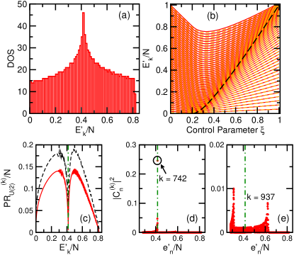
Figure 1: Panel (a): Normalized density of states for $\xi=0.6$, $N=3000$, $\ell=0$. Panel (b): Normalized excitation energies vs $\xi$ for the $U(3)$ total Hamiltonian [Eq. (4)]; $N=100$, $\ell=0$ (full red lines) and $\ell=1$ (dashed orange lines). The separatrix [Eq. (11)] is indicated with the dashed line. Panel (c): Participation ratio of all eigenstates written in the $U(2)$ basis; $\xi=0.6$, $\ell=0$, and $N=300$ (dark curve) and $N=3000$ (light curve). The vertical line marks $E_{\text{ESQPT}}$ obtained from Eq. (11). Panels (d) and (e): squared coefficients $|C_{n}^{(k)}|^{2}$ of the eigenstates $|\psi_{k}\rangle$ written in the $U(2)$ basis vs the energies of the corresponding basis vectors. The eigenstate in (d) is the closest one to the ESQPT critical point and it has $E_{k}^{\prime}/N=0.4168$, and the eigenstate in (e) has energy $E_{k}^{\prime}/N=0.4872$; $\xi=0.6$, $N=3000$, $\ell=0$. Arbitrary units.

III.1 Eigenstates

Figure 1 (b) displays eigenvalues with two angular momenta, $\ell=0$ and $\ell=1$. It is noticeable that states having different angular momentum with energies below the separatrix are degenerate, while this degeneracy is broken for energies above $E_{\text{ESQPT}}$. Thus, the separatrix marks a change in the structure of the eigenstates. Those states with $E_{k}^{\prime}/N<E_{\text{ESQPT}}$ are closer to the eigenstates of the $SO(3)$ Chain, while above the separatrix, they approach the eigenstates of the $U(2)$ Chain Caprio et al. (2008). We verified that this change is reflected in the level of delocalization of the eigenstates $|\psi_{k}\rangle$ written in the $U(2)$ basis,

$$|\psi_{k}\rangle=\sum_{n=\ell}^{N}C_{n}^{(k)}|[N]n\ell\rangle_{k},$$ (12)

where the sum involves either even or odd values of $n$, depending on the $\ell$ parity.

The spreading of an eigenstate in a chosen basis is quantified, for instance, with the participation ratio (PR) Santos et al. (2005); Gubin and Santos (2012); Torres-Herrera and Santos (2013), which is defined as

$$\text{PR}^{(k)}_{U(2)}=\frac{1}{\sum_{n}|C_{n}^{(k)}|^{4}}~{}.$$ (13)

An extended state has a large value of PR, while for $\xi=0$, $\text{PR}^{(k)}_{U(2)}=1$ for every $k$, since the eigenstates coincide with the $U(2)$ basis vectors.

Figure 1 (c) shows the values of the PR for all $\ell=0$ eigenstates for $\xi=0.6$ and two different system sizes. In addition to being small at the borders of the spectrum, the PR also dips abruptly at $E_{\text{ESQPT}}$. At first sight this might be surprising, since this is where the divergence of the density of states occurs [cf. Fig. 1 (a)], so strong mixing and thus delocalized states could have been expected. However, the separatrix marks the point where the eigenstates transition from one dynamical symmetry to the other. Starting at $E_{k}^{\prime}/N=0$ and going up in energy, the point where $E_{k}^{\prime}/N=E_{\text{ESQPT}}$ marks the transition from the $SO(3)$ symmetry to the $U(2)$ symmetry. At this point, the eigenstates become highly localized in the ground state of the $U(2)$ part of the Hamiltonian, that is in the state $|[N]00\rangle$. This strong localization can also be understood from classical considerations, as further discussed in Ref. Santos et al. (a). This sudden change in the value of the PR serves as an alternative method to detect an ESQPT.

To confirm that the localization occurs in the ground state of the $U(2)$ part of $\hat{\cal H}$, we show in Fig. 1 (d), the components $|C_{n}^{(k)}|^{2}$ as a function of the normalized energies of the $U(2)$ basis vector,

$$e^{\prime}_{n}/N=(\langle[N]n\ell|\hat{\cal H}|[N]n\ell\rangle-E_{0})/N,$$ (14)

for the eigenstate that is closest to the separatrix. It is indeed highly localized at $e^{\prime}_{0}/N\sim E_{\text{ESQPT}}$. To contrast this result, we show in Fig. 1 (e), the structure of an eigenstate with $E_{k}^{\prime}/N>E_{\text{ESQPT}}$. The state is delocalized and shows no preference on any $U(2)$ basis vector.

III.2 Fidelity and number of $\tau$ bosons

The ground-state fidelity, $F$, is often used to detect a QPT Zanardi and Paunković (2006). It corresponds to the overlap between two ground states obtained for two values of the control parameter that differ by a very small amount $\delta$,

$$F=\langle\psi_{0}(\xi)|\psi_{0}(\xi+\delta)\rangle.$$ (15)

Away from the QPT critical point, the two ground states are very similar and $F\sim 1$, but at $\xi_{c}$, the ground-state fidelity shows a sudden drop.

The same idea carries over to ESQPTs, except that the abrupt change in $F$ now occurs for two excited states with energies $\sim E_{\text{ESQPT}}$. It reflects the change in the structure of the eigenstates across the separatrix. This is illustrated in Fig. 2 (a), where we show $1-F$ vs $\xi$ for some chosen eigenstates. For each one, $1-F$ peaks at the value of $\xi$ for which $E_{k}^{\prime}/N\sim E_{\text{ESQPT}}$.

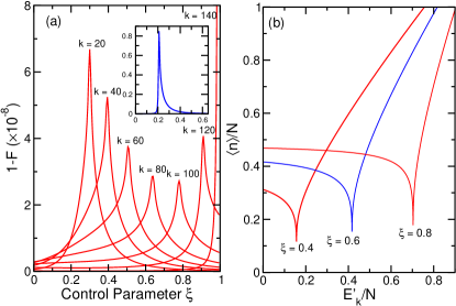
Figure 2: Panel (a): $1-F$ vs $\xi$ for the $U(3)$ model Hamiltonian [Eq. (4)]; $N=300$, $\ell=0$. The values of $k$ for the chosen excited eigenstates are indicated in the figure. For comparison, the inset shows $1-F$ vs $\xi$ for the ground state. Panel (b): Expectation value of the number operator for all eigenstates with $\xi=0.4,0.6$, and $0.8$; $N=3000$, $\ell=0$. Arbitrary units.

The strong localization of the eigenstates at the separatrix in the basis vector with $n=0$ causes the expectation value of the $\tau$ boson number operator, $\langle\psi_{k}|\hat{n}|\psi_{k}\rangle$, to have a pronounced minimum in the critical energy Pérez-Bernal and Álvarez-Bajo (2010), as seen in Fig. 2 (b). Thus, in addition to PR, both $\langle\psi_{k}|\hat{n}|\psi_{k}\rangle$ and the fidelity are alternative quantities capable of detecting the appearance of an ESQPT.

IV Dynamics

Since the eigenstates close to the separatrix are very localized in $|[N]00\rangle$, the evolution of this basis vector under the Hamiltonian (4) must be much slower than the dynamics of other basis vectors, as we show in this section. The speed of the evolution of $U(2)$ basis vectors is therefore another way to detect the presence of an ESQPT.

To examine how fast an initial state $|\Psi(0)\rangle=|[N]n\ell\rangle$ changes in time, we consider the survival probability Borgonovi et al. (2016),

$$S_{p}(t) \equiv \left|\langle\Psi(0)|e^{-i\hat{\cal H}t}|\Psi(0)\rangle\right|^{2}=\left|\sum_{k}|C_{n}^{(k)}|^{2}e^{-iE_{k}t}\right|^{2}$$ (16)

$$= \left|\int dEe^{-iEt}\rho_{n}(E)\right|^{2},$$

where $\rho_{n}(E)=\sum_{k}|C_{n}^{(k)}|^{2}\delta(E-E_{k})$ is the energy distribution of the initial state $|[N]n\ell\rangle$ weighted by the components $|C_{n}^{(k)}|^{2}$. This distribution is referred to as local density of states (LDOS) Borgonovi et al. (2016). Notice that the survival probability is the absolute square of the Fourier transform of the LDOS.

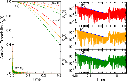
Figure 3: Survival Probability vs time; $\xi=0.6$, $N=5000$. In (a), the initial states from top to bottom have: $n=0$ for the $U(2)$, $U(3)$, and $U(4)$ Hamiltonians; $n=2$ for the $U(2)$, $U(3)$, and $U(4)$ Hamiltonians; and $n=n_{c}$ (the closest $e^{\prime}_{n}/N$ to $E_{\text{ESQPT}}$, apart from $e^{\prime}_{0}/N$) for the $U(2)$, $U(3)$, and $U(4)$ Hamiltonians. Panels (b), (c), and (d) show the long-time evolution of $|\Psi(0)\rangle=|[N]n_{c}0\rangle$ for $U(2)$, $U(3)$, and $U(4)$, respectively; dashed lines give $F(t)\propto 1/t$. Arbitrary units.

In Fig. 3 (a), we compare the evolution of $|[N]00\rangle$, $|[N]2,0\rangle$, and $|[N]n_{c}0\rangle$ under the $U(\nu)$ Hamiltonian (1) with $\nu=1,2$ and $3$. The initial state $|\Psi(0)\rangle=|[N]n_{c}0\rangle$ is the state with the closest value of $e^{\prime}_{n_{c}}/N$ to $E_{\text{ESQPT}}$, with $n_{c}\neq 0$. State $|[N]00\rangle$ has $e^{\prime}_{0}/N\sim E_{\text{ESQPT}}$, because it is highly localized in the eigenstate at the separatrix. As $n$ increases, the states $|[N]n0\rangle$ get more and more delocalized in the energy eigenbasis. The LDOS for $|[N]n_{c}0\rangle$ is approximately symmetrically distributed between eigenstates with $E_{k}^{\prime}/N<E_{\text{ESQPT}}$ and eigenstates with $E_{k}^{\prime}/N>E_{\text{ESQPT}}$, which guarantees that $e^{\prime}_{n_{c}}/N$ is closer to $E_{\text{ESQPT}}$ than $e^{\prime}_{2}/N$ Santos and Pérez-Bernal (2015); Santos et al. (a).

Figure 3 (a) shows that the evolution of $|[N]00\rangle$ is significantly slower than that for the other basis vectors. Overall, the dynamics also accelerates as $\nu$ increases, but in a similar rate for all initial states, which assures the distinctly slow behavior of $|[N]00\rangle$ when compared to other basis vectors.

Figures 3 (b), (c), and (d) depict the long-time decay of the survival probability for the delocalized state $|[N]n_{c}0\rangle$ for $\nu=1,2$ and $3$, respectively. A powerlaw behavior $\propto 1/t$ is found for all three cases. Interestingly, this is also the behavior observed for the integrable XX model with a single excitation Santos et al. (a), which is a spin-1/2 noninteracting model with only nearest-neighbor couplings. The analysis of the LDOS for $|[N]n_{c}0\rangle$ reveals a shape $\propto(\text{constant}-E^{2})^{-1/2}$, whose Fourier transform indeed leads to $S_{p}(t)\propto 1/t$. This shape is also found for the LDOS and for the density of states of the XX model with a single excitation. This suggests a relationship between the short-range XX model and the infinite-range LMG model, which deserves further investigation. Similarities between these two models with respect to the ground state entanglement entropy have been found in Latorre et al. (2005); Barthel et al. (2006).

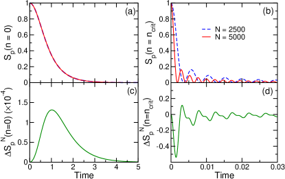
Figure 4: Top panels (a) and (b): Survival probablity vs time for two different system sizes; $N=2500,5000$. Bottom panels (c) and (d): Difference between the survival probability for the same two system sizes vs time. In (a) and (c): $\langle n\rangle=0$; in (b) and (d): $\langle n\rangle=n_{c}$ (the second closest $e^{\prime}_{n}/N$ to $E_{\text{ESQPT}}$). The total Hamiltonian has a $U(3)$ algebraic structure [Eq. (4)] with $\xi=0.6$ and $\ell=0$. Arbitrary units.

A comparison of the decay of the survival probability for different system sizes is provided in Fig. 4 for $|[N]00\rangle$ (a,c) and $|[N]n_{c}0\rangle$ (b,d). In Fig. 4 (a), one sees that before the appearance of oscillations caused by the finite system size, $S_{p}(t)$ practically coincides for different values of $N$. A closer look, in Fig. 4 (c), at the difference $\Delta S_{p}^{N}(t)=S_{p}^{N_{2}}(t)-S_{p}^{N_{1}}(t)$ for two different system sizes $N_{1}$ and $N_{2}$, where $N_{2}>N_{1}$, reveals that the decay is slightly slower for larger $N$. In contrast, the evolution of $|[N]n_{c}0\rangle$ clearly accelerates as $N$ increases, which is evident already in Fig. 4 (b) and further reinforced by the negative values of the difference $\Delta S_{p}^{N}(t)$ in Fig. 4 (d). The slow behavior of $|[N]00\rangle$ is therefore a real effect of the presence of the ESQPT and not a finite size effect.

V Conclusions

We have shown that the presence of an ESQPT can be detected by comparing the speed of the evolution of different $U(\nu)$ basis vectors propagating under a $U(\nu+1)$ Hamiltonian. In the particular case of $\nu=1$, the $U(2)$ Hamiltonian coincides with the spin-1/2 model with infinite-range Ising interaction in the $z$-direction and a transverse field in the $x$-direction. For this model, the initial state that shows a very slow dynamics at the ESQPT critical point is the one where all spins point down in the $z$-direction, which is a state routinely considered in the studies of quench dynamics performed with trapped ions Jurcevic et al. (2014); Richerme et al. (2014).

Our findings demonstrate that the fast evolution expected to be seen in systems with long-range interaction is not a general rule; slow dynamics may be found as well. The behavior of a system out of equilibrium depends on the interplay between its Hamiltonian and its initial state. This has been discussed in Ref. Santos et al. (b) in the context of systems with long-range interaction and has been a recurrent message of our works about nonequilibrium quantum dynamics Torres-Herrera and Santos (2014a, b, c); Torres-Herrera et al. (2014); Távora et al. and thermalization Torres-Herrera and Santos (2013).

VI Acknowledgments

FPB was funded by MINECO grant FIS2014-53448-C2-2-P and by Spanish Consolider-Ingenio 2010 (CPANCSD2007-00042). LFS was supported by the NSF grant No. DMR-1147430. We thank Alejandro Frank for his hospitality at the Centro de Ciencias de la Complejidad (C₃) of the UNAM in Mexico, where part of this work was carried out.

References

- Sachdev (2005) S. Sachdev, in Encyclopedia of Mathematical Physics, edited by J.-P. Francoise, G. Naber, and T. S. Tsun (Elsevier, Amsterdam, 2005).
- Bitko et al. (1996) D. Bitko, T. F. Rosenbaum, and G. Aeppli, Phys. Rev. Lett. 77, 940 (1996).
- Greiner et al. (2002) M. Greiner, O. Mandel, T. Esslinger, T. W. Hänsch, and I. Bloch, Nature 415, 39 (2002).
- Baumann et al. (2010) K. Baumann, C. Guerlin, F. Brennecke, and T. Esslinger, Nature 464, 1301 (2010).
- Caprio et al. (2008) M. Caprio, P. Cejnar, and F. Iachello, Ann. of Phys. 323, 1106 (2008).
- Pérez-Bernal and Iachello (2008) F. Pérez-Bernal and F. Iachello, Phys. Rev. A 77, 032115 (2008).
- Cejnar and Stránský (2008) P. Cejnar and P. Stránský, Phys. Rev. E 78, 031130 (2008).
- Cejnar and Jolie (2009) P. Cejnar and J. Jolie, Progr. Part. Nucl. Phys. 62, 210 (2009).
- Pérez-Fernández et al. (2009) P. Pérez-Fernández, A. Relaño, J. M. Arias, J. Dukelsky, and J. E. García-Ramos, Phys. Rev. A 80, 032111 (2009).
- Pérez-Fernández et al. (2011a) P. Pérez-Fernández, A. Relaño, J. M. Arias, P. Cejnar, J. Dukelsky, and J. E. García-Ramos, Phys. Rev. E 83, 046208 (2011a).
- Brandes (2013) T. Brandes, Phys. Rev. E 88, 032133 (2013).
- Stransky et al. (2014) P. Stransky, M. Macek, and P. Cejnar, Ann. Phys. 345, 73 (2014).
- Winnewisser et al. (2005) B. P. Winnewisser, M. Winnewisser, I. R. Medvedev, M. Behnke, F. C. De Lucia, S. C. Ross, and J. Koput, Phys. Rev. Lett. 95, 243002 (2005).
- Zobov et al. (2006) N. F. Zobov, S. V. Shirin, O. L. Polyansky, J. Tennyson, P.-F. Coheur, P. F. Bernath, M. Carleer, and R. Colin, Chem. Phys. Lett. 414, 193 (2006).
- Larese and Iachello (2011) D. Larese and F. Iachello, J. Mol. Struct. 1006, 611 (2011).
- Larese et al. (2013) D. Larese, F. Pérez-Bernal, and F. Iachello, J. Mol. Struct. 1051, 310 (2013).
- Dietz et al. (2013) B. Dietz, F. Iachello, M. Miski-Oglu, N. Pietralla, A. Richter, L. von Smekal, and J. Wambach, Phys. Rev. B 88, 104101 (2013).
- Zhao et al. (2014) L. Zhao, J. Jiang, T. Tang, M. Webb, and Y. Liu, Phys. Rev. A 89, 023608 (2014).
- Bastarrachea-Magnani et al. (2014) M. A. Bastarrachea-Magnani, S. Lerma-Hernández, and J. G. Hirsch, Phys. Rev. A 89, 032102 (2014).
- (20) J. Chávez-Carlos, M. A. Bastarrachea-Magnani, S. Lerma-Hernández, and J. G. Hirsch, arXiv:1604.00725.
- Pérez-Fernández et al. (2011b) P. Pérez-Fernández, P. Cejnar, J. M. Arias, J. Dukelsky, J. E. García-Ramos, and A. Relaño, Phys. Rev. A 83, 033802 (2011b).
- Engelhardt et al. (2015) G. Engelhardt, V. M. Bastidas, W. Kopylov, and T. Brandes, Phys. Rev. A 91, 013631 (2015).
- Jurcevic et al. (2014) P. Jurcevic, B. P. Lanyon, P. Hauke, C. Hempel, P. Zoller, R. Blatt, and C. F. Roos, Nature 511, 202 (2014).
- Richerme et al. (2014) P. Richerme, Z.-X. Gong, A. Lee, C. Senko, J. Smith, M. Foss-Feig, S. Michalakis, A. V. Gorshkov, and C. Monroe, Nature 511, 198 (2014).
- Zibold et al. (2010) T. Zibold, E. Nicklas, C. Gross, and M. K. Oberthaler, Phys. Rev. Lett. 105, 204101 (2010).
- Araujo-Ferreira et al. (2013) A. G. Araujo-Ferreira, R. Auccaise, R. S. Sarthour, I. S. Oliveira, T. J. Bonagamba, and I. Roditi, Phys. Rev. A 87, 053605 (2013).
- Santos et al. (a) L. F. Santos, M. Távora, and F. Pérez-Bernal, arXiv:1604.04289.
- Santos and Pérez-Bernal (2015) L. F. Santos and F. Pérez-Bernal, Phys. Rev. A 92, 050101 (2015).
- Cejnar and Iachello (2007) P. Cejnar and F. Iachello, J. Phys. A 40, 581 (2007).
- Lipkin et al. (1965) H. J. Lipkin, N. Meshkov, and A. J. Glick, Nucl. Phys. 62, 188 (1965).
- Iachello (1981) F. Iachello, Chem. Phys. Lett. 78, 581 (1981).
- Iachello and Levine (1995) F. Iachello and R. D. Levine, Algebraic Theory of Molecules (Oxford University Press, Oxford, 1995).
- Iachello and Oss. (1996) F. Iachello and S. Oss., J. Chem. Phys. 104, 6956 (1996).
- Pérez-Bernal et al. (2005) F. Pérez-Bernal, L. F. Santos, P. H. Vaccaro, and F. Iachello, Chem. Phys. Lett. 414, 398 (2005).
- Pérez-Bernal and Álvarez-Bajo (2010) F. Pérez-Bernal and O. Álvarez-Bajo, Phys. Rev. A 81, 050101(R) (2010).
- Santos et al. (2005) L. F. Santos, M. I. Dykman, M. Shapiro, and F. M. Izrailev, Phys. Rev. A 71, 012317 (2005).
- Gubin and Santos (2012) A. Gubin and L. F. Santos, Am. J. Phys. 80, 246 (2012).
- Torres-Herrera and Santos (2013) E. J. Torres-Herrera and L. F. Santos, Phys. Rev. E 88, 042121 (2013).
- Zanardi and Paunković (2006) P. Zanardi and N. Paunković, Phys. Rev. E 74, 031123 (2006).
- Borgonovi et al. (2016) F. Borgonovi, F. M. Izrailev, L. F. Santos, and V. G. Zelevinsky, Phys. Rep. 626, 1 (2016).
- Latorre et al. (2005) J. I. Latorre, R. Orús, E. Rico, and J. Vidal, Phys. Rev. A 71, 064101 (2005).
- Barthel et al. (2006) T. Barthel, S. Dusuel, and J. Vidal, Phys. Rev. Lett. 97, 220402 (2006).
- Santos et al. (b) L. F. Santos, F. Borgonovi, and G. L. Celardo, Phys. Rev. Lett. 116, 250402 (2016).
- Torres-Herrera and Santos (2014a) E. J. Torres-Herrera and L. F. Santos, Phys. Rev. A 89, 043620 (2014a).
- Torres-Herrera and Santos (2014b) E. J. Torres-Herrera and L. F. Santos, Phys. Rev. E 89, 062110 (2014b).
- Torres-Herrera and Santos (2014c) E. J. Torres-Herrera and L. F. Santos, Phys. Rev. A 90, 033623 (2014c).
- Torres-Herrera et al. (2014) E. J. Torres-Herrera, M. Vyas, and L. F. Santos, New J. Phys. 16, 063010 (2014).
- (48) M. Távora, E. J. Torres-Herrera, and L. F. Santos, arXiv:1601.05807.