Geometrically disordered network models, quenched quantum gravity, and critical behavior at quantum Hall plateau transitions

Abstract

Recent high-precision results for the critical exponent of the localization length at the integer quantum Hall (IQH) transition differ considerably between experimental ($\nu_{\text{exp}}\approx 2.38$) and numerical ($\nu_{\text{CC}}\approx 2.6$) values obtained in simulations of the Chalker-Coddington (CC) network model. We revisit the arguments leading to the CC model and consider a more general network with geometric (structural) disorder. Numerical simulations of this new model lead to the value $\nu\approx 2.37$ in very close agreement with experiments. We argue that in a continuum limit the geometrically disordered model maps to the free Dirac fermion coupled to various random potentials (similar to the CC model) but also to quenched two-dimensional quantum gravity. This explains the possible reason for the considerable difference between critical exponents for the CC model and the geometrically disordered model and may shed more light on the analytical theory of the IQH transition. We extend our results to network models in other symmetry classes.

Introduction. The integer quantum Hall (IQH) transition Huckestein (1995) is the most prominent example of an Anderson transition, a continuous quantum phase transition driven by disorder and accompanied by universal critical phenomena Evers and Mirlin (2008). Numerous experiments Wei et al. (1988); Koch et al. (1991a, b, 1992); Engel et al. (1993); Wei et al. (1994) demonstrated scaling near the IQH transition characterized by the localization length exponent $\nu$. The most recent and accurate experimental value is $\nu_{\text{exp}}=2.38\pm 0.02$ Li et al. (2005, 2009). A similar value of $\nu$ was observed at the IQH transition in graphene Giesbers et al. (2009), confirming universality at the IQH transition.

The IQH effect is usually modeled by neglecting electron-electron interactions, that is, within the paradigm of Anderson localization Anderson (1958); Abrahams et al. (1979). Existence of delocalized states in disorder-broadened Landau levels, which is necessary to explain the IQH transition, is consistent with the description of the transition by a nonlinear sigma model with a topological term Levine et al. (1983); Weidenmüller (1987), and its two-parameter flow diagram Khmel’nitskiǐ (1983); Pruisken (1985). The critical point of the sigma model should possess conformal invariance and be described by a conformal field theory (CFT) with the central charge $c=0$ Gurarie and Ludwig (2004), due to the use of replicas or supersymmetry (SUSY) to treat disorder averages. However, this fixed point is in the strong coupling regime, and notable attempts at identifying the CFT Zirnbauer (1999); Bhaseen et al. (2000); Tsvelik (2001, 2007) are inconclusive so far.

The IQH transition is related to the problem of disordered Dirac fermions Ludwig et al. (1994). The generic model with random mass, scalar, and gauge potentials is believed to have a fixed point in the universality class of the IQH transition, but this fixed point is not perturbatively accessible. A simplified model where only a random gauge potential is kept, is analytically solvable, and the exact spectrum of multifractal (MF) exponents describing the scaling of the moments of critical wave functions is known Ludwig et al. (1994); de C. Chamon et al. (1996); Mudry et al. (1996); Chamon et al. (1996); Kogan et al. (1996); Castillo et al. (1997).

More recently, alternative approaches to the IQH transition were advanced. One is based on a mapping to a classical model and conformal restriction Bettelheim et al. (2012), and another uses symmetry properties of the sigma model Gruzberg et al. (2011, 2013); Bondesan et al. (2014) to derive exact symmetry properties of the MF spectra at the IQH transition. In spite of these successes, no theoretical predictions for the exponent $\nu$ exist.

Much intuition about the IQH transition, as well as the most accurate numerical estimates for critical exponents, come from a the Chalker-Coddington (CC) network model Chalker and Coddington (1988); Kramer et al. (2005). The model is based on the semiclassical picture of electrons drifting along the equipotential lines of a smooth disorder potential. Tunneling across saddle points of the potential leads to hybridization of the localized states and a possible delocalization. In the CC model this picture is drastically simplified, and all scattering nodes are placed at the vertices of a square lattice. The CC model in various limits can be mapped both to the nonlinear sigma model Read (1991); Zirnbauer (1994), and the random Dirac fermions Ho and Chalker (1996).

The regular geometry of the CC model allows for an easy application of numerical transfer matrix (TM) techniques MacKinnon and Kramer (1983). The most recent and accurate implementations of this method Slevin and Ohtsuki (2009); Obuse et al. (2010); Amado et al. (2011); Obuse et al. (2012); Slevin and Ohtsuki (2012); Nuding et al. (2015), as well as other methods Dahlhaus et al. (2011); Fulga et al. (2011) give the value $\nu_{\text{CC}}$ in the range 2.56–2.62, which is definitely different from the experimental value. One possible source for the discrepancy are electron-electron interactions whose effect on the scaling near the IQH transition has been studied in Refs. Lee and Wang (1996); Wang et al. (2000); Burmistrov et al. (2011). It was shown there that short-range interactions are irrelevant at the IQH critical point, and should not modify the value of $\nu$. This leaves the option that the Coulomb interaction may play a dominant role in experimental systems, but this issue is not fully understood, and remains unresolved.

Here we propose another possible explanation for why the value of $\nu_{\text{CC}}$ differs from $\nu_{\text{exp}}$, namely that the CC model does not capture all types of disorder that are relevant at the IQH transition. Indeed, saddle points that connect the “puddles” of filled electron states do not form a regular lattice, and around each “puddle” there may be any number of them. Taking this into account leads us to consider structurally disordered, or random networks (RNs) that better represent the physics in a smooth disorder potential and strong magnetic field.

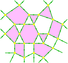
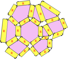
Figure 1.1: Left: a random graph. Right: the corresponding random Manhattan lattice.

Let us list the main results of this paper. (1) We argue that an ensemble of RNs can be mapped in a continuum limit to the problem of free Dirac fermions coupled to random potentials (similar to the CC model) and also to two-dimensional quantum gravity (2DQG). Coupling to 2DQG modifies critical exponents of statistical mechanics models Knizhnik et al. (1988); David (1988); Distler and Kawai (1989); Kazakov (1988); Kazakov and Migdal (1988); Kazakov (1989); Duplantier and Kostov (1990). We suggest that a similar modification happens for RNs. (2) We demonstrate that RNs can be effectively constructed starting with the CC network and appropriately modifying it. The modified RNs can be numerically simulated, and for certain values of parameters specifying the geometric disorder, we obtain the localization length exponent $\nu=2.374\pm 0.018$, in excellent agreement with experiments. (3) We extend these ideas to quantum Hall transitions in symmetry classes C and D in the classification of Refs. Zirnbauer (1996); Altland and Zirnbauer (1997). Properties of these transitions map to classical statistical mechanics models which were studied on random lattices, and for which the shift in critical exponents is given by the KPZ relation Knizhnik et al. (1988); David (1988); Distler and Kawai (1989) from the theory of 2DQG. This fact allows us to predict various exact critical exponents for these transitions.

Random networks. The network models we consider are built on planar directed graphs where every vertex has two incoming and two outgoing edges. The in- and out- edges, also called links of the network, alternate as one goes around a vertex (a node). Such graphs divide the plane into two sets of polygonal faces with opposite orientations of their edges, see Fig. 1.1, left. We will only consider connected graphs, which are exactly the Feynman graphs of zero-dimensional (complex) matrix $\phi^{4}$ theory in the planar (large $N$) limit ’t Hooft (1974); Brezin et al. (1978).

Figure 1.2: Left: an $S$ matrix. Right: the corresponding $R$ matrix.

A state of the network model on a given random graph is represented by a complex vector $Z\in\mathbb{C}^{N}$, where $N$ is the number of edges of the graph, and each component $z_{e}$ corresponds to the complex flux on the edge $e$. The model includes random scattering matrices connecting incoming $z_{1},z_{1^{\prime}}$ and outgoing $z_{2},z_{2^{\prime}}$ fluxes (see Fig. 1.2, left):

$$\Big{(}\!\begin{array}[]{c}z_{2}\\ z_{2^{\prime}}\end{array}\!\!\Big{)}={\cal S}\Big{(}\!\begin{array}[]{c}z_{1}\\ z_{1^{\prime}}\end{array}\!\!\Big{)}=\Big{(}\!\begin{array}[]{cc}te^{i\gamma}&re^{i\gamma^{\prime}}\\ re^{i\gamma}&-te^{i\gamma^{\prime}}\end{array}\!\!\Big{)}\Big{(}\!\begin{array}[]{c}z_{1}\\ z_{1^{\prime}}\end{array}\!\!\Big{)},$$ (1.9)

placed at the vertices. The scattering amplitudes satisfy $t^{2}+r^{2}=1$, and the scattering phases $\gamma$, $\gamma^{\prime}$ are random.

Evolution of the states of the network in discrete time steps is specified by an $N\times N$ unitary matrix $U$ composed of all node scattering matrices Klesse and Metzler (1995). In this description the basic object is the resolvent $(1-e^{-\eta}U)^{-1}$. Its matrix element (a Green function) can be written as a superintegral

$$G(e_{1},e_{2};\eta) =\!\!\!\operatorname*{\mathchoice{\mathchoice{\scalebox{1.3}[1.0]{$\displaystyle\rotatebox{18.0}{$\displaystyle\!\int\!$}$}}{\scalebox{1.3}[1.0]{$\textstyle\rotatebox{18.0}{$\textstyle\!\int\!$}$}}{\scalebox{1.3}[1.0]{$\scriptstyle\rotatebox{18.0}{$\scriptstyle\!\int\!$}$}}{\scalebox{1.3}[1.0]{$\scriptscriptstyle\rotatebox{18.0}{$\scriptscriptstyle\!\int\!$}$}}}{\mathchoice{\scalebox{1.3}[1.0]{$\displaystyle\rotatebox{18.0}{$\displaystyle\!\int\!$}$}}{\scalebox{1.3}[1.0]{$\textstyle\rotatebox{18.0}{$\textstyle\!\int\!$}$}}{\scalebox{1.3}[1.0]{$\scriptstyle\rotatebox{18.0}{$\scriptstyle\!\int\!$}$}}{\scalebox{1.3}[1.0]{$\scriptscriptstyle\rotatebox{18.0}{$\scriptscriptstyle\!\int\!$}$}}}{\mathchoice{\scalebox{1.3}[1.0]{$\displaystyle\rotatebox{18.0}{$\displaystyle\!\int\!$}$}}{\scalebox{1.3}[1.0]{$\textstyle\rotatebox{18.0}{$\textstyle\!\int\!$}$}}{\scalebox{1.3}[1.0]{$\scriptstyle\rotatebox{18.0}{$\scriptstyle\!\int\!$}$}}{\scalebox{1.3}[1.0]{$\scriptscriptstyle\rotatebox{18.0}{$\scriptscriptstyle\!\int\!$}$}}}{\mathchoice{\scalebox{1.3}[1.0]{$\displaystyle\rotatebox{18.0}{$\displaystyle\!\int\!$}$}}{\scalebox{1.3}[1.0]{$\textstyle\rotatebox{18.0}{$\textstyle\!\int\!$}$}}{\scalebox{1.3}[1.0]{$\scriptstyle\rotatebox{18.0}{$\scriptstyle\!\int\!$}$}}{\scalebox{1.3}[1.0]{$\scriptscriptstyle\rotatebox{18.0}{$\scriptscriptstyle\!\int\!$}$}}}}\!\!\!{\cal D}\Psi\,\psi_{e_{1}}{\bar{\psi}}_{e_{2}}e^{-\sum_{e,e^{\prime}}{\bar{\Psi}}_{e}(1-e^{-\eta}U)_{ee^{\prime}}\Psi_{e^{\prime}}}$$ (1.10)

where $e_{1}$, etc., label edges of the graph, and ${\bar{\Psi}}_{e}=({\bar{\phi}}_{e},{\bar{\psi}}_{e})$ is a supervector assigned to the edge $e$, see Refs. Janssen et al. (1999); Cardy (2005) for details. The real part of the parameter $\eta$ plays the role of the imaginary part of the energy (level broadening) in the Hamiltonian description. For our purposes it is sufficient to take $\eta=0$ in what follows.

Formulation of a random network as a lattice model appeared in Ref. Kavalov and Sedrakyan (1987) in connection with the so called sign factor problem in the string representation of the 3D Ising model. This approach was further developed in Refs. Sedrakyan (1999, 2002, 2003); Khachatryan et al. (2009, 2010). Following these references, we connect the midpoint of each edge $e$ “forward” to two other midpoints by two vectors $\xi_{e}$. Then a scattering node is replaced by a rectangle (see Fig. 1.2, right), and we get an alternative representation of the RN as a random Manhattan lattice (ML), see the right part of Fig. 1.1. The action for the RN written as

$$S=\sum_{e}{\bar{\Psi}}_{e}\Psi_{e}-\sum_{e,\xi_{e}}t_{e,\xi_{e}}e^{i\gamma_{e}}{\bar{\Psi}}_{e+\xi_{e}}\Psi_{e}$$ (1.11)

represents hopping of fermions and bosons on the random ML, and the hopping amplitudes take values $r$ and $\pm t$ depending on the vector $\xi_{e}$.

The SUSY method of Refs. Janssen et al. (1999); Cardy (2005) is designed to describe only single-particle problems, while the approach of Refs. Sedrakyan (1999, 2002, 2003); Khachatryan et al. (2009, 2010) allows to consider interacting particles. To this end one uses the second quantization, and the scattering matrices at the nodes are “promoted” to R-matrices acting in the tensor product of Fock spaces attached to edges of the network (see Fig. 1.2, right). On a random ML the R-matrices are represented by the quadrangular faces surrounding the scattering nodes, see Fig. 1.1. The trace of the product of the R-matrices over all nodes of the network gives the partition function. For a general interacting case the SUSY method does not apply, and one has to use replicas to treat disorder. In this paper we do not include interactions and continue to use SUSY. Then writing the trace of the product of the R-matrices in the basis of (super-)coherent states for each of the (super-)Fock spaces on the edges, we obtain the same action (1.11).

Continuum limits. For the regular CC model the ML is a square lattice with vertices labeled by the Cartesian coordinates $x^{\mu}$ ($\mu=1,2$). The vectors $\xi_{e}$ are $\pm\epsilon{\hat{x}}_{\mu}$, where ${\hat{x}}_{\mu}$ are unit vectors, and $\epsilon$ is the lattice spacing. Near the critical point of the CC model ($t_{c}=r_{c}=1/\sqrt{2}$) the variations of the phases $\gamma_{e}$ and the fields $\Psi_{e}$ are slow, and we can pass to a continuum limit by expanding $\Psi_{x+\epsilon{\hat{x}}_{\mu}}\approx(1+\epsilon\partial_{\mu})\Psi_{x}$ and rescaling the fields $\Psi(x)$ in the continuum. In the limit we obtain, as in Ref. Ho and Chalker (1996), the action of the Dirac fermions (and their bosonic partners)

$$S=\!\!\operatorname*{\mathchoice{\mathchoice{\scalebox{1.3}[1.0]{$\displaystyle\rotatebox{18.0}{$\displaystyle\!\int\!$}$}}{\scalebox{1.3}[1.0]{$\textstyle\rotatebox{18.0}{$\textstyle\!\int\!$}$}}{\scalebox{1.3}[1.0]{$\scriptstyle\rotatebox{18.0}{$\scriptstyle\!\int\!$}$}}{\scalebox{1.3}[1.0]{$\scriptscriptstyle\rotatebox{18.0}{$\scriptscriptstyle\!\int\!$}$}}}{\mathchoice{\scalebox{1.3}[1.0]{$\displaystyle\rotatebox{18.0}{$\displaystyle\!\int\!$}$}}{\scalebox{1.3}[1.0]{$\textstyle\rotatebox{18.0}{$\textstyle\!\int\!$}$}}{\scalebox{1.3}[1.0]{$\scriptstyle\rotatebox{18.0}{$\scriptstyle\!\int\!$}$}}{\scalebox{1.3}[1.0]{$\scriptscriptstyle\rotatebox{18.0}{$\scriptscriptstyle\!\int\!$}$}}}{\mathchoice{\scalebox{1.3}[1.0]{$\displaystyle\rotatebox{18.0}{$\displaystyle\!\int\!$}$}}{\scalebox{1.3}[1.0]{$\textstyle\rotatebox{18.0}{$\textstyle\!\int\!$}$}}{\scalebox{1.3}[1.0]{$\scriptstyle\rotatebox{18.0}{$\scriptstyle\!\int\!$}$}}{\scalebox{1.3}[1.0]{$\scriptscriptstyle\rotatebox{18.0}{$\scriptscriptstyle\!\int\!$}$}}}{\mathchoice{\scalebox{1.3}[1.0]{$\displaystyle\rotatebox{18.0}{$\displaystyle\!\int\!$}$}}{\scalebox{1.3}[1.0]{$\textstyle\rotatebox{18.0}{$\textstyle\!\int\!$}$}}{\scalebox{1.3}[1.0]{$\scriptstyle\rotatebox{18.0}{$\scriptstyle\!\int\!$}$}}{\scalebox{1.3}[1.0]{$\scriptscriptstyle\rotatebox{18.0}{$\scriptscriptstyle\!\int\!$}$}}}}\!\!\!d^{2}x\,\bar{\Psi}\big{[}\sigma^{\mu}\big{(}i\overset{\text{\tiny$\leftrightarrow$}}{\partial}_{\mu}+A_{\mu}\big{)}+m\sigma^{3}+V\big{]}\Psi,$$ (1.12)

where $\overset{\text{\tiny$\leftrightarrow$}}{\partial}_{\mu}=(\overset{\text{\tiny$\rightarrow$}}{\partial}_{\mu}-\overset{\text{\tiny$\leftarrow$}}{\partial}_{\mu})/2$, the mass $m\propto r-r_{c}$, and the (random) gauge $A_{\mu}(x)$ and scalar $V(x)$ potentials arise as certain combinations of the random phases $e^{i\gamma_{e}}$.

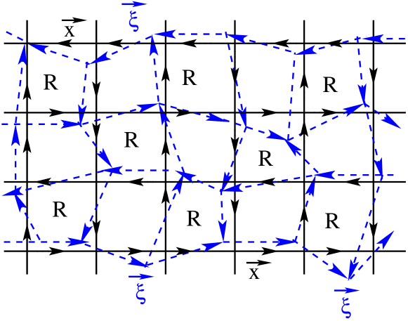
Figure 1.3: Weakly random Manhattan lattice.

Let us now consider the random ML shown in Fig. 1.3. This lattice is not very different from the regular square lattice, its faces are still quadrangles, and we can introduce (curvilinear) coordinates $\xi^{a}$ ($a=1,2$) following the vectors $\xi_{e}$ in a natural way. It is clear that the physics cannot depend on the choice of coordinates, so we can use either $\xi^{a}$ or $x^{\mu}$ coordinates. We can use the formalism of frames (vielbeins) of differential geometry Nakahara (2003) to relate coordinate and orthonormal bases of vectors ${\hat{x}}_{\mu}=e_{\mu}^{a}\partial/\partial\xi^{a}$ and forms $dx^{\mu}=e_{a}^{\mu}d\xi^{a}$, as well as the volume elements $d^{2}x=e\,d^{2}\xi$, where $e=\det e_{a}^{\mu}$. The action (1.12) written in arbitrary coordinates and invariant under coordinate changes becomes

$$S=\!\!\operatorname*{\mathchoice{\mathchoice{\scalebox{1.3}[1.0]{$\displaystyle\rotatebox{18.0}{$\displaystyle\!\int\!$}$}}{\scalebox{1.3}[1.0]{$\textstyle\rotatebox{18.0}{$\textstyle\!\int\!$}$}}{\scalebox{1.3}[1.0]{$\scriptstyle\rotatebox{18.0}{$\scriptstyle\!\int\!$}$}}{\scalebox{1.3}[1.0]{$\scriptscriptstyle\rotatebox{18.0}{$\scriptscriptstyle\!\int\!$}$}}}{\mathchoice{\scalebox{1.3}[1.0]{$\displaystyle\rotatebox{18.0}{$\displaystyle\!\int\!$}$}}{\scalebox{1.3}[1.0]{$\textstyle\rotatebox{18.0}{$\textstyle\!\int\!$}$}}{\scalebox{1.3}[1.0]{$\scriptstyle\rotatebox{18.0}{$\scriptstyle\!\int\!$}$}}{\scalebox{1.3}[1.0]{$\scriptscriptstyle\rotatebox{18.0}{$\scriptscriptstyle\!\int\!$}$}}}{\mathchoice{\scalebox{1.3}[1.0]{$\displaystyle\rotatebox{18.0}{$\displaystyle\!\int\!$}$}}{\scalebox{1.3}[1.0]{$\textstyle\rotatebox{18.0}{$\textstyle\!\int\!$}$}}{\scalebox{1.3}[1.0]{$\scriptstyle\rotatebox{18.0}{$\scriptstyle\!\int\!$}$}}{\scalebox{1.3}[1.0]{$\scriptscriptstyle\rotatebox{18.0}{$\scriptscriptstyle\!\int\!$}$}}}{\mathchoice{\scalebox{1.3}[1.0]{$\displaystyle\rotatebox{18.0}{$\displaystyle\!\int\!$}$}}{\scalebox{1.3}[1.0]{$\textstyle\rotatebox{18.0}{$\textstyle\!\int\!$}$}}{\scalebox{1.3}[1.0]{$\scriptstyle\rotatebox{18.0}{$\scriptstyle\!\int\!$}$}}{\scalebox{1.3}[1.0]{$\scriptscriptstyle\rotatebox{18.0}{$\scriptscriptstyle\!\int\!$}$}}}}\!\!\!d^{2}\xi\,e\,\bar{\Psi}\big{[}\sigma^{\mu}e_{\mu}^{a}\big{(}i\overset{\text{\tiny$\leftrightarrow$}}{\partial}_{a}+A_{a}\big{)}+m\sigma^{3}+V\big{]}\Psi.$$ (1.13)

The action (1.13) is that of 2D fermions interacting with random gauge and scalar potentials as well as random geometry (gravity). In the case of weakly deformed lattices, Eqs. (1.12) and (1.13) are equivalent, they both describe the system on a flat surface. We propose that random frames can account for more complicated situations that correspond to curved surfaces represented by random graphs. In this case we define frames locally, on a given coordinate chart, and then connect them on overlapping charts by transition functions. The result is still given by Eq. (1.13), but now we are supposed to average over “arbitrary” frame configurations. The above arguments leave open the question of the functional measure on random surfaces. We believe that the requirements of diffeomorphism and conformal invariance determine the appropriate measure uniquely, the same way it is fixed in string theory Polyakov (1981).

The need to average observables over random geometry means that our system is coupled to quenched quantum gravity. However, in the SUSY formalism the partition function of a disordered system is always unity (implying $c=0$ for the CFT of the critical point), and there is no difference between quenched and annealed gravity.

It is known that 2DQG modifies critical exponents of a CFT placed on a fluctuating surface in the way given by the KPZ relation Knizhnik et al. (1988); David (1988); Distler and Kawai (1989). The relation has been verified by solutions of critical models of statistical mechanics (related to the so-called minimal CFTs Belavin et al. (1984)) defined on random graphs Kazakov (1988); Kazakov and Migdal (1988); Kazakov (1989); Duplantier and Kostov (1990). When $c=0$, as for Anderson transitions and critical percolation, the relation is

$$\Delta=(\sqrt{1+24\Delta_{0}}-1)/4,$$ (1.14)

where $\Delta_{0}$ ($\Delta$) are chiral dimensions of operators on a flat (fluctuating) surface. Whether this relation can explain the difference between $\nu_{\text{CC}}$ and $\nu_{\text{exp}}$ is to be seen. However, Eq. (1.14) should be applicable to properly defined MF exponents of critical wave functions at the IQH transition, as well as other 2D Anderson transitions.

Figure 1.4: Top: opening a node. Bottom: The resulting modifications of the CC network.

Construction and simulation of RNs. To simulate RNs numerically, we adopt the following construction. Starting with the regular CC network, at each node we set $t=0$ with probability $p_{0}$, $t=1$ with probability $p_{1}$, and leave the node unchanged with probability $p_{c}=1-p_{0}-p_{1}$. The modified nodes with $t=0$ ($t=1$) are “open” in the horizontal (vertical) direction, and opening a node changes the four adjacent square faces into two triangles and one hexagon, see Fig. 1.4. Repeated opening of nodes can produce tilings of the plane by polygons with arbitrary numbers of edges. At the same time, our construction still allows us to use the transfer matrix (TM) of the CC model, but with modified $t$ and $r$ amplitudes.

To maintain statistical isotropy of the model, we choose $p_{0}=p_{1}$. In this case we expect that the critical point is still given by the value $t_{c}^{2}=1/2$ for the unchanged nodes. Moreover, in this paper we fix $p_{0}=p_{1}=p_{c}=1/3$.

We simulate the modified networks on strips of different width $M$ (the number of nodes per column) varying from $20$ to $200$, the length $L=5\cdot 10^{6}$, and a range of the parameter $x$ which encodes deviations of $t$ from $t_{c}$ . We use the LU decomposition of TMs Press et al. (2007). Since $t$ and $r$ appear in the denominators of the matrix elements of TMs, making them zero is a singular procedure, related to the disappearance of two horizontal channels upon opening a node in the vertical direction. To overcome this difficulty, for every open node we take either $t$ or $r$ to be equal to $\varepsilon\ll 1$. We then look at how the resulting Lyapunov exponents depend on $\epsilon$. We found that the results saturate at $\varepsilon=10^{-5}$, and there are no changes when reducing $\epsilon$ to $10^{-7}$. For even smaller $\varepsilon$ the results start changing again. This is to be expected because the large differences of values in the entries of TMs cause numerical instabilities for the LU decomposition. We have chosen $\varepsilon=10^{-6}$ for our calculations.

The smallest Lyapunov exponent $\gamma$ is expected to have the following finite-size scaling behavior:

$$\gamma M=\Gamma[M^{1/\nu}u_{0}(x),M^{y}u_{1}(x)].$$ (1.15)

Here $u_{0}(x)$ is the relevant field and $u_{1}(x)$ the leading irrelevant field. The relevant field vanishes at the critical point, and $y<0$. The fitting procedure of our numerical results, as well as the error analysis are presented in the Supplementary material. The results of the analysis are

$$\nu =2.374\pm 0.018, y=-0.35\pm 0.05.$$ (1.16)

This value of $\nu$ is surprisingly close to $\nu_{\text{exp}}$, which suggests that the structural disorder is, indeed, a relevant perturbation that modifies the critical behavior.

Other symmetry classes. Network models can be constructed for all 10 symmetry classes of disordered systems identified in Refs. Zirnbauer (1996); Altland and Zirnbauer (1997). Superconductors with broken time-reversal invariance in 2D can exhibit QH transitions where the spin (class C) Kagalovsky et al. (1999); Senthil et al. (1999) and thermal (class D) Senthil and Fisher (2000) conductivities jump in quantized units. The ideas developed above apply to network models for these transitions. In addition, both SQH and TQH are simpler than the IQH since many of their properties can be determined from mappings to classical models.

The regular network in class C was mapped to classical bond percolation on a square lattice Gruzberg et al. (1999); Beamond et al. (2002); Mirlin et al. (2003). Many exact results are known for classical percolation. Thus, the mapping has lead to a host of exact critical properties at the SQH transition Gruzberg et al. (1999); Mirlin et al. (2003); Cardy (2000); Subramaniam et al. (2006, 2008); Bondesan et al. (2012); Bhardwaj et al. (2015). The mapping was extended to network models in class C on arbitrary graphs Cardy (2005).

The graphs relevant for our study are shown in Fig. 1.5. For a given RN we draw the dual bipartite graph with dots on the shaded faces and crosses on the empty faces of the original RN. The dual graph forms a random quadrangulation of the plane. We now dissect all quadrangles by diagonals connecting the dots, and remove the crosses and all edges connected to them. This results in a lattice (Fig. 1.5, right) on which the classical bond percolation should be considered.

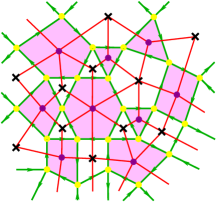
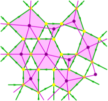
Figure 1.5: Left: original RN and its dual. Right: percolation lattice.

Critical bond percolation on random quadrangulations (or their duals) was considered in Ref. Kazakov (1989), and it was shown that the KPZ relation (1.14) is valid in this case. We believe that the SQH transition on RNs lies in the same universality class, and that Eq. (1.14) can be applied to all critical exponents obtained in Refs. Gruzberg et al. (1999); Mirlin et al. (2003); Subramaniam et al. (2006, 2008); Bondesan et al. (2012); Bhardwaj et al. (2015). This includes, in particular, the dimension of the “two-leg” operator that determines the localization length exponent $\nu$ as well as a few MF exponents.

The TQH transition in class D can also be described and simulated by a network model Cho and Fisher (1997); Chalker et al. (2002); Merz and Chalker (2002); Mildenberger et al. (2007). Its effective field theory (without geometric disorder) is given by the Majorana fermions with random mass, the same theory that describes the critical Ising model with a weak bond disorder Senthil and Fisher (2000); Bocquet et al. (2000). The random mass is a marginally irrelevant perturbation, and critical exponents at the transition are given by their Ising model values. When the model is coupled to 2DQG, we still should consider the quenched situation, and the critical exponents should be modified according to Eq. (1.14), see Janke et al. (2006) and references therein.

Discussion and outlook. The geometric disorder that we simulate by a modified CC model can be viewed as randomness in the heights $V$ of the saddle points in the disorder potential. Indeed, it is known that (at zero energy) $t^{2}=(1+e^{-V})^{-1}$ Fertig and Halperin (1987). Our choice of $t$ is described by the tri-modal distribution $P(V)=p_{0}\delta(V-2\ln\varepsilon)+p_{c}\delta(V-V_{0})+p_{0}\delta(V+2\ln\varepsilon).$ Previous studies of random $V$ Lee et al. (1993); Evers and Brenig (1998) focused instead on the uniform distribution in the interval $V\in[-W,W]$ or the bimodal distribution $P(V)=[\delta(V-W)+\delta(V+W)]/2$. No choice of $W$ gives our type of randomness when $p_{c}>0$. However, for $p_{c}=0$ our distribution becomes bimodal, and describes classical percolation with $\nu=4/3$. The other extreme, $p_{c}=1$, gives the regular CC model. Since we only simulated the point $p_{c}=1/3$, we cannot distinguish the following three possibilities: 1) a novel fixed point at a finite $p_{c}$, 2) a crossover from percolation to CC criticality, 3) a line of fixed points. We plan to study other values of $p_{c}$ to determine which scenario is actually realized.

We also plan to simulate RNs in classes C and D, and try to solve the classical percolation problem on relevant graphs using matrix models techniques. We will, furthermore, consider the problem of Dirac fermions in an Abelian random gauge potential coupled to 2DQG, and determine the MF spectrum of the wave functions in order to test the applicability of the KPZ relation (1.14).

In summary, we have considered the possibility that a certain type of geometric (structural) disorder, previously missed in the study of the IQH transition, may change the universality class. Our numerical simulations support this idea. We have also proposed that the proper framework for a field-theoretic description of this type of disorder is provided by 2DQG coupled to matter fields. These ideas can be applied to other 2D Anderson transitions.

Supplemental material
Network model for plateau transitions in the quantum Hall effect

We calculate numerically the localization length index $\nu$ in the Chalker-Coddington (CC) network suitably modified to represent a random network. We use one relevant field and one irrelevant field in the fitting procedure. The results lead to the value $\nu\approx 2.37$ for the modified model, in very close agreement with experiments.

2.1 Model description

For the calculation of critical indices we used the transfer-matrix method developed in MacKinnon and Kramer (1981, 1983). To calculate the smallest Lyapunov exponent of the CC-model it is necessary to calculate a product $T_{L}=\prod_{j=1}^{L}M_{1}U_{1j}M_{2}U_{2j}$ of layers of transfer matrices $M_{1}U_{1j}M_{2}U_{2j}$ corresponding to two columns $M_{1}$ and $M_{2}$ of vertical sequences of 2x2 scattering nodes,

$$M_{1}=\leavevmode\hbox to85.92pt{\vbox to69.79pt{\text{[drawing]}}} {B^{1}} {0} {0} {0} {B^{1}} {0} {0} {0} {B^{1}} \left.\vbox{\hrule height=33.64389pt,depth=33.64389pt,width=0.0pt}\right) \left(\vbox{\hrule height=33.64389pt,depth=33.64389pt,width=0.0pt}\right. {B^{1}} {0} {0} {0} {B^{1}} {0} {0} {0} {B^{1}} \left.\vbox{\hrule height=33.64389pt,depth=33.64389pt,width=0.0pt}\right) \left(\vbox{\hrule height=33.64389pt,depth=33.64389pt,width=0.0pt}\right.$$ (2.1)

and

$$M_{2}=\leavevmode\hbox to98.48pt{\vbox to82.26pt{\text{[drawing]}}} {B^{2}_{22}} {0} {0} {B^{2}_{21}} {0} {B^{2}} {0} {0} {B^{2}} {0} {B^{2}_{12}} {0} {0} {B^{2}_{11}} \left.\vbox{\hrule height=39.878pt,depth=39.878pt,width=0.0pt}\right) \left(\vbox{\hrule height=39.878pt,depth=39.878pt,width=0.0pt}\right. {B^{2}_{22}} {0} {0} {B^{2}_{21}} {0} {B^{2}} {0} {0} {B^{2}} {0} {B^{2}_{12}} {0} {0} {B^{2}_{11}} \left.\vbox{\hrule height=39.878pt,depth=39.878pt,width=0.0pt}\right) \left(\vbox{\hrule height=39.878pt,depth=39.878pt,width=0.0pt}\right.$$ (2.2)

with

$$B^{1}=\begin{pmatrix}1/t&r/t\\ r/t&1/t\end{pmatrix}\qquad\text{and}\qquad B^{2}=\begin{pmatrix}1/r&t/r\\ t/r&1/r\end{pmatrix}$$ (2.3)

The $U$-matrices have a simple diagonal form with independent phase factors $U_{nm}=\exp{(i\alpha_{n})}\,\delta_{nm}$ for $U=U_{1j}$ and $U_{2j}$. Here $t$ and $r$ are the transmission and reflection amplitudes at each node of the regular lattice which are parameterized by

$$t=\frac{1}{\sqrt{1+e^{2x}}}\qquad\text{and}\qquad r=\frac{1}{\sqrt{1+e^{-2x}}}.$$ (2.4)

The parameter $x$ corresponds to the Fermi energy measured from the Landau band center scaled by the Landau band width (with the critical point at $x=0$). The phases $\alpha_{n}$ are random variables uniformly distributed in the range $[0,2\pi)$, reflecting that the phase of an electron approaching a saddle point of the random potential is arbitrary.

To simulate random networks (RNs) numerically, we remove scattering nodes by opening them in horizontal or vertical direction with probabilities $p_{0}$ and $p_{1}$ by adopting the following construction. Starting with the regular CC network, at each node we set $t=\varepsilon\ll 1$ with probability $p_{0}$, $t=\sqrt{1-\varepsilon^{2}}$ with probability $p_{1}$, and leave the node unchanged with probability $p_{c}=1-p_{0}-p_{1}$. Here the small number $\varepsilon$ is chosen as $\varepsilon=10^{-6}$: We found that the results saturate already at $\varepsilon=10^{-5}$, and there are no changes when reducing $\varepsilon$ to $10^{-7}$. For even smaller $\varepsilon$ the results start changing again due to precision issues of the numerics.

Furthermore, in this report we use $p_{0}=p_{1}=p_{c}=1/3$.

2.2 The fitting procedure

For the scaling behavior of the Lyapunov exponent $\gamma$ near the critical point we expect the finite size dependence

$$\gamma\cdot M=\Gamma(M^{1/\nu}u_{0},M^{y}\,u_{1}),$$ (2.5)

Here we have taken into account the relevant field with exponent $\nu$ and the leading irrelevant field with exponent $y$. $M$ is the number of $2\times 2$ blocks in the transfer matrices ($=$ half the number of horizontal channels of the lattice), $u_{0}=u_{0}(x)$ is the relevant field and $u_{1}=u_{1}(x)$ the leading irrelevant field. It is known that the relevant field vanishes at the critical point, and that $y<0$.

On the left hand side of Eq. (2.5) we use the numerical results for the eigenvalues of $T_{L}$, where we are particularly interested in the eigenvalue closest to 1. The Lyapunov exponent $\gamma$ is the smallest positive eigenvalue of

$$\lim_{L\to\infty}\frac{\log[T_{L}T_{L}^{\dagger}]}{2L}\ ,$$ (2.6)

which we calculate for various combinations of the parameter $x$ and the lattice width $M$. The right hand side of (2.5) is expanded in a series in $x$ and powers of $M$, and the expansion coefficients are obtained from a fit. Some coefficients in this expansion vanish due to a symmetry argument Slevin and Ohtsuki (2009). If $x$ is replaced by $-x$ we see from (2.4) that $t$ turns into $r$ and vice versa. Due to the periodic boundary conditions the lattice is unchanged. Therefore the left hand side of (2.5) is invariant under the sign change of $x$. Hence the right hand side must be even in $x$. That renders $u_{0}(x)$ and $u_{1}(x)$ either even or odd in $x$. For the Chalker Coddington network the critical point is at $x=0$. This lets us choose $u_{0}(x)$ odd and $u_{1}(x)$ even. The fit now should use as few coefficients as possible while reproducing the data as closely as possible.

The scaling function $\Gamma$ in the right side of (2.5) is expanded in the fields $u_{0}$ and $u_{1}$ yielding

$$\begin{split}\Gamma(&u_{0}(x)M^{1/\nu},u_{1}(x)M^{y})=\Gamma_{00}+\Gamma_{01}u_{1}M^{y}+\Gamma_{20}u_{0}^{2}M^{2/\nu}\\ &+\Gamma_{02}u_{1}^{2}M^{2y}+\Gamma_{21}u_{0}^{2}u_{1}M^{2/\nu}M^{y}+\Gamma_{03}u_{1}^{3}M^{3y}\\ &+\Gamma_{40}u_{0}^{4}M^{4/\nu}+\Gamma_{22}u_{0}^{2}M^{2/\nu}u_{1}^{2}M^{2y}+\Gamma_{04}u_{1}^{4}M^{4y}+\dots\end{split}$$ (2.7)

We further expand $u_{0}$ and $u_{1}$ in powers of $x$ as was done, for example, in Refs. Slevin and Ohtsuki (2009); Amado et al. (2011):

$$u_{0}(x)=x+\sum_{k=1}^{\infty}a_{2k+1}x^{2k+1}\quad\text{and}\quad u_{1}(x)=1+\sum_{k=1}^{\infty}b_{2k}x^{2k}.$$ (2.8)

In Eq. (2.7) we retained only terms that are even in $x$. Because of the ambiguity in the overall scaling of the fields, the leading coefficient in Eq. (2.8) can be chosen to be 1.

2.3 Weights and Errors

The left hand side of Eq. (2.5) is determined by the results of numerical simulations of the random network model. Following Ref. Amado et al. (2011) we have produced large ensembles of the Lyapunov exponent $\gamma$ by simulating many disorder realizations for many combinations of $x$ and $M$. We calculated $624$ disorder realizations for any combination of $M=20,40,60,80,100,120,140,160,180,200$ and $x=0.08/12\cdot[0,1,2,3,4,5,6,7,8,9,10,11,12]$ for fixed $L=5\,000\,000$. Our goal is to check whether the central limit theorem (CLT) Tutubalin (1965) also works in the case of randomness of the network or not. Fig. 2.1 shows the distribution of the Lyapunov exponent for $M=60$ and $x=0.02$ being nicely described by a Gaussian which demonstrates the validity of CLT.

In the fitting procedure, the weight of each such $\gamma$ is given by the reciprocal of the variance of the corresponding ensemble. On the right hand side of Eq. (2.5) the fitting formula depending on $x$ and $M$ is used. The coefficients of the expansion and the critical exponents are the fitting coefficients.

The fits are performed in several steps. First a weighted nonlinear least square fit based on a trust region algorithm with specified regions for each parameter is applied. The resulting parameters are used in a further weighted nonlinear least square fit based on a Levenberg-Marquardt algorithm. Here no limits are imposed on the fit parameters. The last step is repeated until the resulting parameters stop changing.

2.4 Evaluation of fits

The next step is the evaluation of the fit results. We present several methods to do this.

Very common is the ${\chi^{2}}$-test. $\chi^{2}$ is given by

$$\chi^{2}=\sum_{i}\frac{(y_{i}-f_{i})^{2}}{\sigma^{2}}$$ (2.9)

where $f_{i}$ is the value predicted by the fit and $y_{i}$ the measured value. $\sigma$ is given by the standard deviation. As our fit contains large ensembles of data points for the same $(x,M)$ coordinates, $\chi^{2}=0$ is not possible, actually it will be large due to the huge number of data points. The way to deal with this behavior is to consider the ratio $\chi^{2}$/degrees of freedom. The expectation value for this ratio is 1 for an ideal fit. The degrees of freedom is the number of data points in the fit minus the number of fit parameters.

Deviations from 1 are evaluated by use of the cumulative probability $P(\tilde{\chi}^{2}<\chi^{2})$ which is the probability of observing – just for statistical reasons – a sample statistic with a smaller $\chi^{2}$ value than in our fit. A small value of $P$, i.e. a large value of the complement $Q:=1-P$ is taken as indicative for a good fit. However, values of $P$ lower than $1/2$ indicate problems in the estimation of the error bars of the individual data points.

Another criterion is based on the width of the confidence intervals. This quantifies the quality of the prediction for a single parameter. We use 95% confidence intervals which means that for repeated independent generation of the same amount of data and application of the same kind of data analysis the resulting confidence intervals contain the true parameter values in 95% of the cases.

A most sensitive criterion is the Akaike information criterion (AIC) Akaike (1974). AIC is founded on information theory; Akaike found a formal relationship between Kullback-Leibler information and likelihood theory. This finding makes it possible to combine estimation (i.e., maximum likelihood or least squares) and model selection under a unified optimization framework.

Unlike in the case of hypothesis testing, AIC does not assume that the correct model is among the tested models. AIC rather offers a relative estimate of the information lost when a given model is used to represent the process that generates the data. This way, given a collection of models, AIC ranks those models if they are based on the same data. In this case a comparison to the best model can be calculated easily. In case a different data base has been used, the models cannot be ranked or compared.

For the calculations presented in this article we have been using the AICc, which is a small sample version of AIC or, more precisely, a second order bias correction. AICc is also valid if $k$ is not small compared to $n$, where $n$ denotes the sample size and $k$ denotes the number of parameters, and is given by

$$\text{AICc}=\text{AIC}+\frac{2k(k+1)}{n-k-1}.$$ (2.10)

This formula holds exactly if the model is univariate, linear, and has normally-distributed residuals, but may in other cases still be used unless a more precise correction is known. Further details on the AIC and the AICc can be found in Kenneth P. Burnham (2002).

The AIC can be expressed in terms of $\chi^{2}$:

$$\text{AIC}=2k+\chi^{2}-2C$$ (2.11)

Here $2C$ is a constant (dependent on the set of data points) that can be omitted because for comparisons we only need differences of AICc’s.

For comparing models, the AIC (and the AICc) are used in the following way. Suppose, we have $l$ models with AIC₁, …AIC_l. The model with the smallest AICc — let us call it AIC_min, — is the favorite one. The relative probability of model $j$ compared to the model with AIC_min is

$$\exp\frac{\text{AIC}_{min}-\text{AIC}_{j}}{2}.$$ (2.12)

Note that the exponential expression is smaller than one.

The last criterion we present is the sum of residuals. It is given by $\mathit{res}=\sum_{j}\mathit{res}_{j},\;\mathit{res}_{j}=y_{j}-f_{j}$. The sum of residuals should be small compared to the number of degrees of freedom. The residuals plotted should look like noise around zero. If the residuals significantly deviate from zero, we expect that the fit function is not correct.

Figure 2.1: Distribution of Lyapunov exponents in the ensemble of calculations with 624 elements for chain length $L=5\,000\,000$, $M=60$ and $x=0.02$.

2.5 Results

In Fig.2.1 we present an example of the distribution of Lyapunov exponents for fixed width $M$, parameter $x$ and chain length $L$. This distribution defines the data point and its accuracy for the combination $(x,M)$. The reciprocal of the variance is used as the weight the data point carries in the fitting procedure.

Figure 2.2: Plot of the smallest eigenvalue of the transfer matrix times $M$ (number of blocks) depending on the distance $x$ from the critical point. The $x$-values divide the interval $[0,0.08]$ into 12 equal parts.

In Fig.2.2 we present the product $M\gamma$ (the left-hand side of Eq. (2.5)) versus $x$ for various values of the width $M$. The corresponding fitting parameters are presented in the table below.

Our best fitting results have been obtained by expanding $\Gamma$ up to second order in $u_{0}$ and $u_{1}$ (2.7), and expanding $u_{0}$ ($u_{1}$) up to the third (second) order in $x$. We found the following coefficients and goodness of fit parameters:

Coefficients (confidence bounds 95%):

$$\Gamma_{00}=\; \quad 0.864 (0.856 ,0.871)$$

$$\Gamma_{01}=\; \quad 0.0898 (-0.071 ,0.250)$$

$$\Gamma_{02}=\; \quad 0.976 (0.907 ,1.046)$$

$$\Gamma_{20}=\; \quad 0.312 (0.302 ,0.321)$$

$$a_{3}=\; \quad 0.293 (-0.221 ,0.807)$$

$$b_{2}=\; -0.255 (-0.460 ,-0.049)$$

$$\nu=\; \quad 2.374 (2.356 ,2.391)$$

$$y=\; -0.356 (-0.407 ,-0.306)$$

Goodness of fit parameters:

$$\chi^{2}\text{\,: } 81192.5$$

degrees of freedom (dof)  : $$81112$$

$$\chi^{2}/\text{dof\,: } 1.001$$

$$P\text{\,: } 0.554$$

AICc : $$-556356.5$$

sum of residuals : $$181.86$$

Figure 2.3: This figure presents a plot of the residuals. The $x$-axis shows the scaling parameter $x$ and the $y$-axis the residuals. For each pair $(x,M)$ the corresponding residuals are summed up and the result is shown in the plot. By inspection the x-axis is at the center of the scattered residuals. This indicates that there is no systematic deviation between the data points and the model equation.

The degrees of freedom have been calculated from the number of data points $624\cdot 13\cdot 10$ minus 8, the number of fit parameters. We see $\chi^{2}/$dof is close to 1 and the cumulative probability $P=0.554$ is close to $1/2$, marking a good fit result. The sum of residuals is small compared to the number of degrees of freedom. As can be seen in Fig.2.3, the residuals are distributed around zero as judged by the eye. All this indicates that the fit is reliable and the data agree with the model equation.

Fits with two irrelevant fields are clearly discouraged by the Akaike criterion. Those models produce a (relative) Akaike coefficient of at least $\text{AICc}=-556340$. Therefore their relative likelihood is about 0.0003.