Spectral determinants and quantum theta functions

Abstract

It has been recently conjectured that the spectral determinants of operators associated to mirror curves can be expressed in terms of a generalization of theta functions, called quantum theta functions. In this paper we study the symplectic properties of these spectral determinants by expanding them around the point $\hbar=2\pi$, where the quantum theta functions become conventional theta functions. We find that they are modular invariant, order by order, and we give explicit expressions for the very first terms of the expansion. Our derivation requires a detailed understanding of the modular properties of topological string free energies in the Nekrasov–Shatashvili limit. We derive these properties in a diagrammatic form. Finally, we use our results to provide a new test of the duality between topological strings and spectral theory.

1 Introduction

Topological string theory was introduced in the ’80s as a simplified model of string theory which captures information on the background geometry ts1 . Since then, this theory has led to many new results in mathematical physics.

Originally this model was defined only perturbatively by a formal asymptotic expansion. When the background geometry is a toric Calabi-Yau (CY), one can compute the coefficients of this series at any order in perturbation theory akmv2 ; ko ; kz ; bcov . Many aspects of the large order behavior of this formal expansion have been studied in a series of papers starting with the seminal paper mmopen and leading to several insights on a possible non–perturbative definition of the theory gikm ; msw1 ; ps ; dmpnp ; mmnp ; asv ; cesv1 ; mpp ; cesv2 ; gmz . Recently, by using the so–called Fermi gas formalism, a non–perturbative completion of topological strings on toric CY has been proposed. This formalism was first introduced in the context of ABJM theory mp and further extended to topological string theory in ghm , by using the insights from hmmo ; km .

In the non–perturbative formulation of ghm one associates a trace class, positive definite operator, $\hat{\rho}_{X}$, to any toric Calabi-Yau 3-fold $X$ whose mirror geometry has genus one (the higher genus generalization was later worked out in cgm2 ) . Physically, this operator corresponds to the density matrix of an ideal Fermi gas with a positive and discrete spectrum. Such a spectrum can be elegantly organized into the so–called spectral (or Fredholm) determinant

$$\Xi({\kappa},\hbar)=\det\left(1+\kappa\hat{\rho}_{X}\right).$$ (1.1)

In ghm it has been conjectured an explicit expression for this spectral determinant in terms of (un)refined Gopakumar-Vafa invariants of X. At the orbifold point ($\kappa=0$), the spectral determinant, denoted by $\Xi_{X}(\kappa,\hbar)$, has the following expression

$$\Xi({\kappa},\hbar)=1+\sum_{N\geq 1}\kappa^{N}Z(N,\hbar),$$ (1.2)

where $Z(N,\hbar)$ can be identified with the partition function of a one dimensional ideal Fermi gas with N particles. The proposal of ghm is that $Z(N,\hbar)$ provides a non-perturbative definition for the topological string partition function where the string coupling $g_{s}$ is identified with the inverse of the Planck constant $\hbar$. This gives a duality between topological string theory and quantum mechanics similarly to the AdS/CFT correspondence adscft where on the AdS side we have topological string theory on toric CYs while the role of the CFT is played by a one dimensional Fermi gas.

In this formalism the perturbative expansion of standard (or unrefined) topological strings emerges when we study the t’ Hooft limit of the gas, namely

$$N,\hbar\to\infty,\qquad{N\over\hbar}\quad\text{fixed}.$$ (1.3)

However, there are important non–perturbative corrections to the t’ Hooft limit (1.3) which can be detected by looking at the thermodynamic limit of the gas

$$N\to\infty,\qquad{\hbar}\quad\text{fixed}.$$ (1.4)

These non-perturbative corrections are determined by the so–called Nekrasov–Shatashvili (NS) limit of the refined topological string hmmo ; ghm . By combining the results of ghm ; kama with the Cauchy identity mp , one can write $Z(N,\hbar)$ as a matrix model whose ’t Hooft expansion reproduces the perturbative expansion of topological strings in the conifold frame mz ; kmz .

The explicit expression for the spectral determinant in terms of enumerative invariants proposed in ghm ; cgm2 is based on an expansion at the large radius point of the moduli space where

$$\kappa\gg 0.$$ (1.5)

However, to fully understand $\Xi(\kappa,\hbar)$ at a generic point of the moduli space one would need a Gopakumar-Vafa-like resummation gv away from the large radius point. Although, there are evidences and concrete examples to believe that such a resummation should exist ghmabjm ; oz , at present it is not known. Nevertheless, there are some special cases, called the ”maximally supersymmetric” cases, where it is possible to write down a closed form expression for the spectral determinant in terms of hypergeometric and conventional theta functions cgm ; ghm . In these cases we have a good control of the spectral determinant over the full moduli space. Such a simplification occurs for instance when $\hbar=2\pi$. Therefore in our formalism the simplest regime is a quantum regime where $\hbar=2\pi$ and not the classical one.

The strategy in this paper is to study $\Xi(\kappa,\hbar)$ at a generic point of the moduli space (parametrized by $\kappa$) by performing an expansion around the special value $\hbar=2\pi$

$$\Xi({\boldsymbol{\kappa}},\hbar)=\sum_{n\geq 0}{1\over n!}{{\rm d}^{n}\Xi({\boldsymbol{\kappa}},2\pi)\over{\rm d}^{n}\hbar}(\hbar-2\pi)^{n}.$$ (1.6)

At each order in the expansion one can write down a closed form expression for the spectral determinant in term of unrefined and NS free energies where the $n^{\rm th}$ order is completely determined by the free energies $F_{g}$ and $F_{h}^{\rm NS}$ with $g,h\leq n$. In this paper we will work out in details the very first few terms in this expansion (1.6).

It is well known we ; abk that different points in the moduli space correspond to different choices of symplectic frames. The transformations properties of the unrefined free energies under such a change of frame have been worked out in detail in we ; abk where it was shown that the unrefined free energies transform as a wave function while moving around the moduli space. In this paper we will see that a similar behavior holds also for the NS free energies. By using these considerations we argue that, order by order in the $\hbar-2\pi$ expansion (1.6), the spectral determinant is invariant under a change of symplectic frame.

This paper is organized as follows. In sections 2 and 3 we review some of the results concerning the special geometry of toric Calabi-Yaus and the conjecture of ghm . In section 4 we organize the modular properties of the Nekrasov-Shatashvili free energies by using diagrammatic rules and in section 5 we study the expansion of the spectral determinant around $\hbar=2\pi$. In section 6 we use these results to give further evidence for the topological string/quantum mechanics duality proposed in ghm .

2 Special Geometry

We consider a toric Calabi Yau 3-fold X whose mirror geometry is encoded in a Riemann surface of genus $g_{\Sigma}$:

$$W_{X}({\rm e}^{x},{\rm e}^{p},{\boldsymbol{\kappa}})=0,\quad x,p\in{\mathbb{C}},$$ (2.7)

where

$${\boldsymbol{\kappa}}=\left\{\kappa_{1},\cdots,\kappa_{g_{\Sigma}}\right\},$$ (2.8)

are the complex deformation parameters describing the geometry (2.7), see hkrs ; hkp for more details.

Let $\mathcal{A}_{I},\mathcal{B}_{I}$ be a symplectic basis of cycle for the above surface

$${{\cal A}}_{I}\cap{{\cal B}}_{J}\propto\delta_{IJ},\qquad{{\cal A}}_{I}\cap{{\cal A}}_{J}=0,\qquad{{\cal B}}_{I}\cap{{\cal B}}_{J}=0,\qquad I,J=1,\cdots,g_{\Sigma}.$$ (2.9)

The classical periods for the geometry (2.7) are given by

$$\Pi_{A_{I}}({\boldsymbol{\kappa}})=\oint_{{{\cal A}}_{I}}p(x){{\rm d}x},\quad\Pi_{B_{I}}({\boldsymbol{\kappa}})=\oint_{{{\cal B}}_{I}}p(x){{\rm d}x},$$ (2.10)

where $p(x)$ is determined by (2.7). For sake of simplicity we omit the dependence on ${\boldsymbol{\kappa}}$ in $p(x)$. The classical mirror map $\epsilon_{I}$ and the genus zero free energy $F_{0}$ of topological string on X, can be computed from these periods as ckyz

$$\epsilon_{I}({\boldsymbol{\kappa}})=-\Pi_{A_{I}}({\boldsymbol{\kappa}}),\qquad\partial_{\epsilon_{I}}F_{0}({\boldsymbol{\kappa}})=-\Pi_{B_{I}}({\boldsymbol{\kappa}}).$$ (2.11)

Sometimes we refer to $\epsilon_{I}$ as classical Kähler parameter. When performing a modular transformation of the cycles

$$\left(\begin{array}[]{c}{{\cal B}}\\ {{\cal A}}\end{array}\right)\rightarrow\left(\begin{array}[]{cc}A&B\\ C&D\end{array}\right)\left(\begin{array}[]{c}{{\cal B}}\\ {{\cal A}}\end{array}\right),\quad\begin{pmatrix}A&B\\ C&D\end{pmatrix}\in{\rm Sp}(2g,{\mathbb{Z}})$$ (2.12)

the classical periods transform according to abk

$$\left(\begin{array}[]{c}{\Pi_{B}}\\ {\Pi_{A}}\end{array}\right)\rightarrow\left(\begin{array}[]{cc}A&B\\ C&D\end{array}\right)\left(\begin{array}[]{c}{\Pi_{B}}\\ {\Pi_{A}}\end{array}\right).$$ (2.13)

This is what it is called a change of symplectic frame. In the following we will use the term symplectic (or modular) transformation to refer to such a change of frame.

In acdkv , based on earlier works adkmv ; mirmor ; mirmor2 ; mt ; Bonelli:2011na , it was argued that one can quantize the curve (2.7) by promoting $x$ and $p$ to operators fulfilling the standard commutation relation

$$\left[\hat{x},\hat{p}\right]={\rm i}\hbar.$$ (2.14)

The differential $p(x){\rm d}x$ is then promoted to a quantum differential

$$p(x,\hbar){\rm d}x$$ (2.15)

fulfilling

$$W({\rm e}^{\hat{x}},{\rm e}^{\hat{p}},{\boldsymbol{\kappa}})\left(\exp\left[{{1\over\hbar}\int^{x}p(y,\hbar){\rm d}y}\right]\right)=0.$$ (2.16)

The corresponding quantum periods are defined by

$$\Pi_{A_{I}}(\hbar,{\boldsymbol{\kappa}})=\oint_{{{\cal A}}_{I}}p(x,\hbar){{\rm d}x},\quad\Pi_{B_{I}}(\hbar,{\boldsymbol{\kappa}})=\oint_{{{\cal B}}_{I}}p(x,\hbar){{\rm d}x}.$$ (2.17)

These periods are related to the so-called Nekrasov–Shatashvili (NS) free energy (3.39) through

$$\epsilon_{I}(\hbar,{\boldsymbol{\kappa}})=-\Pi_{A_{I}}(\hbar,{\boldsymbol{\kappa}}),\qquad\hbar\partial_{\epsilon_{I}}F^{\rm NS}({\hbar,\boldsymbol{\kappa}})=-\Pi_{B_{I}}(\hbar,{\boldsymbol{\kappa}}).$$ (2.18)

In hkrs , based on earlier work huangNS ; mirmor , it was argued that

$$\Pi_{A_{I}}(\hbar,{\boldsymbol{\kappa}})= \sum_{n\geq 0}\Pi_{A_{I}}^{(n)}({\boldsymbol{\kappa}})\hbar^{2n},\qquad\Pi_{B_{I}}(\hbar,{\boldsymbol{\kappa}})= \sum_{n\geq 0}\Pi_{B_{I}}^{(n)}({\boldsymbol{\kappa}})\hbar^{2n}$$ (2.19)

with

$$\Pi_{A_{I}}^{(n)}({\boldsymbol{\kappa}}) =\mathsf{D}_{1}^{(n)}({\boldsymbol{\kappa}})\Pi_{A_{I}}^{(0)}+\mathsf{D}_{2}^{(n)}({\boldsymbol{\kappa}})\Pi_{A_{I}}^{(0)},$$ (2.20)

$$\Pi_{B_{I}}^{(n)}({\boldsymbol{\kappa}}) =\mathsf{D}_{1}^{(n)}({\boldsymbol{\kappa}})\Pi_{B_{I}}^{(0)}+\mathsf{D}_{2}^{(n)}({\boldsymbol{\kappa}})\Pi_{B_{I}}^{(0)}.$$

where

$$\Pi_{A,B}^{(0)}=\Pi_{A,B}({\boldsymbol{\kappa}})$$ (2.21)

denote the classical periods (2.10) and $\mathsf{D}_{i}^{(n)}({\boldsymbol{\kappa}})$ are differential operators of order $i$. We give a concrete example in appendix A.2. It follows that the quantum periods transform according to

$$\left(\begin{matrix}\hbar\partial_{{\boldsymbol{\epsilon}}}F^{\rm NS}\\ {\boldsymbol{\epsilon}}\end{matrix}\right)\to\left(\begin{matrix}A&B\\ C&D\end{matrix}\right)\left(\begin{matrix}\hbar\partial_{{\boldsymbol{\epsilon}}}F^{\rm NS}\\ {\boldsymbol{\epsilon}}\end{matrix}\right).$$ (2.22)

To make contact with the results of ghm ; cgm2 it is useful to introduce

$${t}_{I}({\boldsymbol{\kappa}},\hbar)= -{1\over(2\pi{\rm i})^{1/2}}\mathcal{C}_{IJ}\epsilon_{J}({\boldsymbol{\kappa}},\hbar),\quad I,J=1,\cdots g_{\Sigma}.$$ (2.23)

The matrix $\mathcal{C}_{IJ}$ is a $g_{\Sigma}\times g_{\Sigma}$ matrix which can be read off from the toric data of $X$ as explained in cgm2 ; kpsw . We also use

$${T}_{I}({\boldsymbol{\kappa}},\hbar)= {1\over(2\pi{\rm i})^{1/2}}\epsilon_{I}({\boldsymbol{\kappa}},\hbar),\quad I,J=1,\cdots g_{\Sigma}.$$ (2.24)

It follows that

$$\left(\begin{matrix}\hbar\partial_{{\bf t}}F^{\rm NS}\\ 2\pi{\rm i}{\bf t}\end{matrix}\right)\to\left(\begin{matrix}A&B\\ C&D\end{matrix}\right)\left(\begin{matrix}\hbar\partial_{{\bf t}}F^{\rm NS}\\ 2\pi{\rm i}{\bf t}\end{matrix}\right),$$ (2.25)

$$\left(\begin{matrix}\hbar\partial_{{\bf T}}F^{\rm NS}\\ 2\pi{\rm i}{\bf T}\end{matrix}\right)\to\left(\begin{matrix}A&B\\ C&D\end{matrix}\right)\left(\begin{matrix}\hbar\partial_{{\bf T}}F^{\rm NS}\\ 2\pi{\rm i}{\bf T}\end{matrix}\right).$$ (2.26)

Depending on the kind of computation it is more convenient to use ${\bf T},{\bf t}$ or $\boldsymbol{\epsilon}$.

3 Spectral determinant and topological strings

In this section we will review some aspects of the work ghm and its generalization to mirror curves of higher genus cgm2 . A pedagogical review of this conjecture and its implications has been presented in mmnew .

The starting point is the quantization of the mirror curve (2.7) which leads to $g_{\Sigma}$ trace class operators (see kama for a rigorous mathematical proof)

$$\hat{\rho}_{i}(\tilde{\boldsymbol{\kappa}}_{i}),\quad i=1,\cdots,g_{\Sigma},$$ (3.27)

where

$$\tilde{\boldsymbol{\kappa}}_{i}=\left\{\kappa_{1},\cdots,\kappa_{i-1},\kappa_{i+1},\cdots,\kappa_{g_{\Sigma}}\right\}.$$ (3.28)

The operators (3.27) have a discrete spectrum which can be elegantly organized into a generalized spectral determinant

$$\Xi_{X}({\boldsymbol{\kappa}},\hbar)={\rm det}\left(1+\kappa_{1}\hat{\rho}_{1}\right){\rm det}\left(1+\kappa_{2}\hat{\rho}_{2}\Big{|}_{\kappa_{1}=0}\right)\cdots{\rm det}\left(1+\kappa_{g_{\Sigma}}\hat{\rho}_{g_{\Sigma}}\Big{|}_{\kappa_{1}=\cdots=\kappa_{g_{\Sigma}-1}=0}\right).$$ (3.29)

More precisely, the spectrum of the operators $\hat{\rho}_{i}(\tilde{\boldsymbol{\kappa}}_{i})$ is determined by vanishing locus of $\Xi_{X}({\boldsymbol{\kappa}},\hbar)$ as explained in cgm2 . In the case of a genus one mirror curve the generalized spectral determinant (3.29) becomes the standard Fredholm determinant

$$\Xi_{X}(\kappa,\hbar)=\det(1+\kappa\hat{\rho}_{X})=\prod_{n}\left(1+\kappa{\rm e}^{-E_{n}}\right),$$ (3.30)

where ${\rm e}^{-E_{n}}$ are the eigenvalues of $\hat{\rho}_{X}$.

As an example we consider the anti canonical bundle over $\mathbb{CP}^{2}$. For this geometry the mirror curve (2.7) reads

$$W(x,p,\kappa)={\rm e}^{x}+{\rm e}^{p}+{\rm e}^{-x-p}+\kappa,$$ (3.31)

and the corresponding quantum operator is

$$\hat{\rho}_{{\mathbb{P}}^{2}}=\left({\rm e}^{\hat{x}}+{\rm e}^{\hat{p}}+{\rm e}^{-\hat{x}-\hat{p}}\right)^{-1}.$$ (3.32)

An important achievement of ghm ; cgm2 is that one can compute (3.29) explicitly in term of (refined) Gopakumar-Vafa (GV) invariants of X. These topological invariants determine (3.29) through the so–called topological string grand potential $J_{X}({\boldsymbol{\mu}},\hbar)$ which was first introduced in mp and then further studied in hmo ; hmo2 ; hmo3 ; cm ; hmmo ; hoo ; ghm ; gkmr ; hatsuda . More precisely we define

$$\mathsf{J}_{X}({\boldsymbol{\mu}},\hbar)= {1\over 12\pi\hbar}a_{IJK}t_{I}(\hbar)t_{J}(\hbar)t_{K}(\hbar)+{2\pi\over\hbar}b_{I}t_{I}(\hbar)+{\hbar\over 2\pi}b_{I}^{\rm NS}t_{I}(\hbar)+F^{\rm GV}({4\pi^{2}\over{\rm i}\hbar},{2\pi\over\hbar}{\bf t}(\hbar)+{\rm i}\pi B)$$ (3.33)

$$+\mathsf{J}_{b}({\boldsymbol{\mu}},\hbar)+\mathsf{J}_{c}({\boldsymbol{\mu}},\hbar)+A(\hbar).$$

We use

$$\boldsymbol{\kappa}={\rm e}^{\boldsymbol{\mu}}$$ (3.34)

and

$$F^{\rm GV}(g_{s},{\bf t}(\hbar))=\sum_{g\geq 0}\sum_{\bf d}\sum_{w=1}^{\infty}{1\over w}n_{g}^{{\bf d}}\left(2\sin{w{\rm i}g_{s}\over 2}\right)^{2g-2}{\rm e}^{-w{\bf d}\cdot{\bf t}(\hbar)},$$ (3.35)

where $n_{g}^{{\bf d}}$ are the standard GV invariants of $X$. This quantity is sometimes called the instanton part of the topological string free energy whose full expression reads

$$F(g_{s},{\bf t}(\hbar))=\sum_{g\geq 0}g_{s}^{2g-2}F_{g}({\bf t}(\hbar))={1\over 6({\rm i}g_{s})^{2}}a_{IJK}t_{I}(\hbar)t_{J}(\hbar)t_{K}(\hbar)+b_{I}t_{I}(\hbar)+F^{\rm GV}(g_{s},{\bf t}(\hbar)).$$ (3.36)

We denote by $F_{g}$ the genus g free energies of standard topological strings .

The refined invariants $N^{{\bf d}}_{j_{L},j_{R}}$ appear through the functions $\mathsf{J}_{c}$ and $\mathsf{J}_{b}$. These are defined as

$$\mathsf{J}_{b}({\boldsymbol{\mu}},\hbar)=\sum_{{\boldsymbol{\ell}}\geq{\bf 1}}(\boldsymbol{\ell}\cdot{\bf t})b_{\boldsymbol{\ell}}{\rm e}^{-\boldsymbol{\ell}\cdot{\bf t}(\hbar)},\quad\mathsf{J}_{c}({\boldsymbol{\mu}},\hbar)=\sum_{{\boldsymbol{\ell}}\geq{\bf 1}}c_{\boldsymbol{\ell}}{\rm e}^{-\boldsymbol{\ell}\cdot{\bf t}(\hbar)},$$ (3.37)

with

$$b_{\boldsymbol{\ell}}= -\frac{1}{4\pi}\sum_{j_{L},j_{R}}\sum_{\boldsymbol{\ell}=\boldsymbol{d}w}\sum_{\boldsymbol{d}}N^{\boldsymbol{d}}_{j_{L},j_{R}}\frac{\sin\frac{\hbar w}{2}(2j_{L}+1)\sin\frac{\hbar w}{2}(2j_{R}+1)}{w^{2}\sin^{3}\frac{\hbar w}{2}}.$$ (3.38)

$$c_{\boldsymbol{\ell}}= -\hbar^{2}{\partial\over\partial\hbar}\left({b_{\boldsymbol{\ell}}\over\hbar}\right).$$

Generically, the geometry of the mirror curve to toric CYs is parametrized by two set of variables: the ”true” moduli (3.28) and the mass parameters $m_{i}$. In this paper we set these parameters to the particular value which guarantee the vanishing of the corresponding algebraic mirror map. As a consequence one has a particularly simple relation between the $b_{\boldsymbol{\ell}}$’s and $c_{\boldsymbol{\ell}}$’s coefficients given in (3.38) (see ghm ; gkmr for more details).

Notice that $\mathsf{J}_{b}$ is closely related to the NS free energy

$$\hbar^{-1}F^{\rm NS}(\hbar,{\bf t}(\hbar))=\sum_{g\geq 0}\hbar^{2g-2}F_{g}^{\rm NS}({\bf t}(\hbar)) =-{1\over 6\hbar^{2}}a_{IJK}t_{I}(\hbar)t_{J}(\hbar)t_{K}(\hbar)-b^{\rm NS}_{I}t_{I}$$ (3.39)

$$-\sum_{j_{L},j_{R}}\sum_{w,{\bf d}}N^{{\bf d}}_{j_{L},j_{R}}\frac{\sin\frac{{\rm i}\hbar w}{2}(2j_{L}+1)\sin\frac{\hbar w}{2}(2j_{R}+1)}{2\hbar w^{2}\sin^{3}\frac{\hbar w}{2}}{\rm e}^{-w{\bf d}\cdot{\bf t}(\hbar)}.$$

The parameter $B$ appearing in (3.33) is a geometrical parameter which is related to the canonical class of the geometry X, we refer to it as B field hmmo . The function $A(\hbar)$ in (3.33) is the so-called constant map contribution bcov and it is necessary to guarantee the correct normalization of the spectral determinant, namely

$$\Xi_{X}({\boldsymbol{0}},\hbar)=1.$$ (3.40)

The conjecture of ghm ; cgm2 states that

$$\Xi_{X}({\boldsymbol{\kappa}},\hbar)=\sum_{{\bf n}\in{\mathbb{Z}}^{g_{\Sigma}}}\exp\left(\mathsf{J}_{X}(\boldsymbol{\mu}+2\pi{\rm i}{\bf n},\hbar)\right).$$ (3.41)

Moreover

$$\Xi_{X}({\boldsymbol{\kappa}},\hbar)=\sum_{{N_{1}}\geq{0}}\cdots\sum_{{N_{g_{\Sigma}}}\geq{0}}Z({\bf{N}},\hbar)\kappa_{1}^{N_{1}}\cdots\kappa_{g_{\Sigma}}^{N_{g_{\Sigma}}}$$ (3.42)

where $Z({\bf N},\hbar)$ defines the non–perturbative partition function of topological strings on $X$. As explained in ghm it corresponds to the partition function of an ideal Fermi gas. This conjecture and its consequences have been further tested in kama ; mz ; kmz ; ho2 ; gkmr ; oz ; hw ; wzh . In hm ; fhma this conjecture has been used to obtain exact quantization conditions for the integrable systems of Goncharov and Kenyon and for the relativistic Toda lattice. In bgt , by using recent developments in the context of Painlevé equations gil ; bes ; ilt , a proof of the conjecture in a limiting case was provided.

The sum in (3.41) can be implemented formally and we write

$$\Xi_{X}({\boldsymbol{\kappa}},\hbar)=\exp\left(\mathsf{J}_{X}(\boldsymbol{\mu}+2\pi{\rm i}{\bf n},\hbar)\right)\Theta_{X}({\boldsymbol{\kappa}},\hbar),$$ (3.43)

where

$$\Theta_{X}({\boldsymbol{\kappa}},\hbar)=\sum_{{\bf n}\in{\mathbb{Z}}^{g_{\Sigma}}}\exp\left[\mathsf{J}_{X}(\boldsymbol{\mu}+2\pi{\rm i}{\bf n},\hbar)-\mathsf{J}_{X}(\boldsymbol{\mu},\hbar)\right]$$ (3.44)

defines the quantum theta function whose zeros determine the spectrum of the operators (3.27). Moreover, according to the conjecture, its inclusion cures the non–analyticity of the grand potential in such a way that the resulting spectral determinant is an analytic function in $\boldsymbol{\kappa}$. As explained in ghm ; cgm2 , the grand potential (3.33) leads to an explicit expression for the quantum theta function in terms of (refined) GV invariants valid near the large radius region of the moduli space and, for real values of $\hbar$, it has good convergence properties. However away from this region very little is known. There are few exceptions to this, among them we have the self-dual point with $\hbar=2\pi$. For this value the quantum theta function becomes a conventional theta function an one can write a closed form expression for (3.43) at any point of the moduli space in terms of hypergeometric and theta functions.

In this paper we explore the other regions of the moduli space away from the large radius point by performing an expansion around this special value of $\hbar=2\pi$. As first pointed out in a related context cgm , it is straightforward to see that for this value of $\hbar$ only genus zero and genus one free energies

$$F_{0}({\bf t}(\hbar)),F_{1}({\bf t}(\hbar)),F_{1}^{\rm NS}({\bf t}(\hbar))$$ (3.45)

contribute to (3.36) and (3.39). For toric Calabi-Yaus these are typically known in closed form in term of Meijer and hypergeometric functions. Hence we can write down a closed form expression for $\Xi_{X}({\boldsymbol{\kappa}},2\pi)$ at any point of the moduli space in term of these special functions. Let us define

$${F}_{g}=F_{g}({\bf t}(0)), \quad{F}_{g}^{\rm NS}=F_{g}^{\rm NS}({\bf t}(0)),$$ (3.46)

$$\widehat{F}_{g}=F_{g}({\bf t}(2\pi)), \quad\widehat{F}_{g}^{\rm NS}=F_{g}^{\rm NS}({\bf t}(2\pi)).$$

In ghm ; cgm2 it was argued that ${\bf t}(2\pi)$ can be obtained from ${\bf t}(0)$ by switching the sign in some of the complex deformations parameter describing the mirror geometry to X. Therefore, under a change of symplectic frame

$${\bf{t}}(2\pi),\quad\widehat{F}_{g},\quad\widehat{F}_{g}^{\rm NS},$$ (3.47)

have the same tranformation properties of

$${\bf{t}}(0),\quad F_{g},\quad F_{g}^{\rm NS}.$$ (3.48)

It was found in ghm ; cgm2 that, when $\hbar=2\pi$, the spectral determinant takes a particularly simple form, namely

$$\Xi_{X}({\boldsymbol{\kappa}},2\pi)=\exp\left[-{1\over 4\pi^{2}}\widehat{F}_{0}+\widehat{F}_{1}-\widehat{F}_{1}^{\rm NS}\right]\Theta_{0,\beta}(\widehat{\boldsymbol{\xi}},\widehat{\tau}),$$ (3.49)

where

$$\widehat{\xi}_{M}=-{\mathcal{C}_{JM}\over 4\pi^{2}}\left\{{\partial^{2}\widehat{F}_{0}\over\partial t_{J}\partial t_{K}}t_{K}-{\partial\widehat{F}_{0}\over\partial t_{J}}\right\}={1\over 4\pi^{2}}\left({\partial^{2}\widehat{F}_{0}\over\partial T_{M}\partial T_{K}}T_{K}-{\partial\widehat{F}_{0}\over\partial T_{M}}\right),\qquad M=1,\cdots,g_{\Sigma}$$ (3.50)

$$\widehat{\tau}_{LM}={1\over 2\pi{\rm i}}\mathcal{C}_{JL}\mathcal{C}_{KM}{\partial^{2}\widehat{F}_{0}\over\partial t_{J}\partial t_{K}}={1\over 2\pi{\rm i}}\partial_{T_{L}}\partial_{T_{M}}\widehat{F}_{0},\qquad L,M=1,\cdots,g_{\Sigma}.$$

Notice that $\widehat{\tau}$ is modular parameter of the spectral curve (2.7) therefore ${\rm Im}(\widehat{\tau})>0$. The constant $\beta$ in (3.49) can be computed explicitly in term of $b_{I},b_{J}^{\rm NS},a_{IJK}$ ghm ; gkmr . The theta function $\Theta_{\alpha,\beta}$ is defined as em

$$\Theta_{0,\beta}(\widehat{\boldsymbol{\xi}},\widehat{\tau})=\exp\left[{1\over 4\pi^{2}}{\left({\boldsymbol{T}}\partial_{\boldsymbol{T}}{\widehat{F}_{0}}-{1\over 2}{\boldsymbol{T}}^{2}\partial_{\boldsymbol{T}}^{2}\widehat{F}_{0}\right)}\right]\vartheta\left[\begin{array}[]{cc}\boldsymbol{0}\\ \boldsymbol{\beta}\end{array}\right](\widehat{\boldsymbol{\xi}},\widehat{\tau}),$$ (3.51)

where

$$\vartheta\left[\begin{array}[]{cc}\boldsymbol{\alpha}\\ \boldsymbol{\beta}\end{array}\right]\left({\boldsymbol{v}},\tau\right)=\sum_{{\boldsymbol{n}}\in{\mathbb{Z}}^{2}}\exp\left[~{}^{t}({\boldsymbol{n}}+{\boldsymbol{\alpha}}){\tau{\rm i}\pi}({\boldsymbol{n}}+{\boldsymbol{\alpha}})+2\pi{\rm i}({\boldsymbol{v}}+{\boldsymbol{\beta}})\cdot\left({\boldsymbol{n}}+{\boldsymbol{\alpha}}\right)\right].$$ (3.52)

Moreover the Kähler parameters in (3.50) are evaluated at $\hbar=2\pi$.

As first noticed in cgm , the spectral determinant evaluated at $\hbar=2\pi$ is similar to the leading order of the background independent partition function proposed in bde ; eynard ; em . However, there are two main differences. The first one consists in the fact that the theta function has now an oscillatory behavior with no need to impose additional constraints on the moduli as was required in bde ; eynard ; em . This improvement of the convergence properties is related to the fact that to compute the spectral determinant (3.41) one has to sum over imaginary shifts of the moduli, whereas in bde ; em ; eynard the sum runs over real shifts. Moreover the proposal of bde ; em ; eynard is defined by a formal $1/N$ ’t Hooft like expansion (1.3) which misses important non-perturbative effects in ${\rm e}^{-N}$ that in our formalism are determined by the NS free energies. These differences become even more important at higher orders in the expansion (1.6). In particular the NS quantities do not simply factorize as in (3.52) but they mix with the unrefined free energies and their derivatives. We work out some explicit example in section 5 and in appendix B.

Notice that $F^{\rm GV}$, $\mathsf{J}_{b}$ and $\mathsf{J}_{c}$ in (3.33) are ill defined for $\hbar=2\pi$ due to the presence of some poles. However when we sum them up these poles disappear and we are left with a well defined quantity: the grand potential $J_{X}$. This is the so-called HMO cancellation mechanism hmo2 and to guarantee such a mechanism the NS free energies play a crucial role.

As we will see in the next section, the genus one free energy $F^{\rm NS}_{1}$ is modular invariant. Therefore it follows from the computations of em , that $\Xi({\boldsymbol{\kappa}},2\pi)$ is invariant under (2.12) up to a phase and change of characteristic in the theta function. Let us review how this goes. By using

$$\left(\begin{matrix}\hbar\partial_{{\bf T}}\widehat{F}_{0}\\ 2\pi{\rm i}{\bf T}\end{matrix}\right)\to\left(\begin{matrix}A&B\\ C&D\end{matrix}\right)\left(\begin{matrix}\hbar\partial_{{\bf T}}\widehat{F}_{0}\\ 2\pi{\rm i}{\bf T}\end{matrix}\right),$$ (3.53)

it is straightforward to see that the combination

$$\widehat{F}_{0}-{1\over 2}{\boldsymbol{T}}\partial_{\boldsymbol{T}}{\widehat{F}_{0}},$$ (3.54)

is symplectic invariant. Similarly we have

$$-{N^{2}\over 2}\left({\boldsymbol{T}}\partial_{\boldsymbol{T}}{\widehat{F}_{0}}-{\boldsymbol{T}}^{2}\partial_{\boldsymbol{T}}^{2}\widehat{F}_{0}\right)\to -{N^{2}\over 2}\left({\boldsymbol{T}}\partial_{\boldsymbol{T}}{\widehat{F}_{0}}-{\boldsymbol{T}}^{2}\partial_{\boldsymbol{T}}^{2}\widehat{F}_{0}\right)+{\rm i}\pi\widehat{\boldsymbol{\xi}}\widehat{\mathcal{K}}\widehat{\boldsymbol{\xi}},$$ (3.55)

$$\widehat{\boldsymbol{\xi}}\to \widehat{\boldsymbol{\xi}}\left(C\widehat{\tau}+D\right)^{-1},$$

$$\widehat{\tau}\to \left(A\widehat{\tau}+B\right)\left(C\widehat{\tau}+D\right)^{-1},$$

where

$$\widehat{\mathcal{K}}=-C\left(C\widehat{\tau}+D\right)^{-1}.$$ (3.56)

In particular one can show that, up to an overall phase factor, we have em

$${\rm e}^{\widehat{F}_{1}}\vartheta\left[\begin{array}[]{cc}\boldsymbol{0}\\ \boldsymbol{\beta}\end{array}\right](\widehat{\boldsymbol{\xi}},\widehat{\tau})\to{\rm e}^{\widehat{F}_{1}}{\rm e}^{-\pi{\rm i}\widehat{\boldsymbol{\xi}}\widehat{\mathcal{K}}\widehat{\boldsymbol{\xi}}}\vartheta\left[\begin{array}[]{cc}\boldsymbol{\gamma}\\ \boldsymbol{\delta}\end{array}\right](\widehat{\boldsymbol{\xi}},\widehat{\tau}),$$ (3.57)

with

$$C\boldsymbol{\delta}=D\boldsymbol{\gamma}+{1\over 2}(CD^{T})_{d},$$ (3.58)

$$\boldsymbol{\beta}=A\boldsymbol{\delta}-B\boldsymbol{\gamma}+{1\over 2}(AB^{T})_{d},$$

where $(M)_{d}$ is a vector whose components are the diagonal element of the matrix $M$. Hence from (3.54),(3.55) and (3.57) it follows that $\Xi({\boldsymbol{\kappa}},2\pi)$ is invariant under a change of symplectic frame (2.12), up to a phase factor and a change of characteristic in the theta function.

Notice that the $\widehat{\tau}$ matrix in (3.50) reads

$$\widehat{\tau}_{IJ}=\partial_{\epsilon_{I}}\partial_{\epsilon_{J}}\widehat{F}_{0}.$$ (3.59)

Similarly we define

$$\tau_{IJ}=\partial_{\epsilon_{I}}\partial_{\epsilon_{J}}F_{0},$$ (3.60)

where

$$F_{0}=F_{0}({\bf t}(0)).$$ (3.61)

According to (2.13) we have

$$\tau\to\left({A\tau+B}\right)\left(C\tau+D\right)^{-1}.$$ (3.62)

4 Change of symplectic frame

We are interested in studying the spectral determinant at a generic point of the moduli space. As explained in we ; abk different points in the moduli space correspond to different choices of symplectic frames (2.12). Therefore we have to study the symplectic properties of the quantities which determine the spectral determinant $\Xi({\boldsymbol{\kappa}},\hbar)$, in particular the standard and NS free energies (3.36), (3.39). For the standard free energy (3.36) these properties have been worked out in abk ; emo where it was shown than these can be formulated in a compact way thanks to the wave function behavior of the unrefined partition function. A discussion of the modular properties of the NS free energies has been done in hk ; huangNS . In the following we organize them by using diagrammatic rules in a wave function like behavior which is controlled by the same action of the unrefined theory.

4.1 The Nekrasov–Shatashvili free energies

In this section we study how the NS free energies transform under (2.12). For that we need to integrate $\Pi_{B_{I}}(\hbar,{\boldsymbol{\kappa}})$ by carefully taking into account the $\hbar$ dependence in the quantum A period ${\boldsymbol{\epsilon}}(\hbar,{\boldsymbol{\kappa}})$. We will use

$$F^{\rm NS}_{g}= F^{\rm NS}_{g}({\bf t}(0)),$$ (4.63)

$$\epsilon_{I}(\hbar)= \sum_{n\geq 0}\hbar^{2n}\epsilon^{(n)}_{I}.$$

Then we have ($\partial_{I}=\partial_{\epsilon_{I}}$)

$$\hbar\partial_{I}F^{\rm NS}(\hbar,{\bf t}(\hbar))= ({\partial_{I}}F^{\rm NS}_{0}+\hbar^{2}\left({\partial_{I}}F^{\rm NS}_{1}+{\epsilon_{J}}^{(1)}\tau_{JI}\right)$$ (4.64)

$$+\hbar^{4}\left({\epsilon_{J}}^{(2)}\tau_{IJ}+{\epsilon_{J}}^{(1)}{\epsilon_{K}}^{(1)}{1\over 2}\partial_{K}\partial_{J}\partial_{I}F_{0}+{\epsilon_{K}}^{(1)}\partial_{K}\partial_{I}F_{1}^{\rm NS}+\partial_{I}F_{2}^{\rm NS}\right)+\mathcal{O}\left(\hbar^{6}\right)$$

where we denote by $\partial_{I}F^{\rm NS}_{g}$ the derivative w.r.t. the classical period ${\epsilon_{I}}^{(0)}$ evaluated at $\hbar=0$. Since the index structure of (4.64) is clear we will simply denote it by

$$\hbar\partial F^{\rm NS}= \partial F^{\rm NS}_{0}+\hbar^{2}\left(\partial F^{\rm NS}_{1}+\epsilon^{(1)}\tau\right)$$ (4.65)

$$+\hbar^{4}\left(\epsilon^{(2)}\tau+\left(\epsilon^{(1)}\right)^{2}{1\over 2}\partial^{3}F_{0}+\epsilon^{(1)}\partial^{2}F_{1}^{\rm NS}+\partial F_{2}^{\rm NS}\right)+\mathcal{O}\left(\hbar^{6}\right).$$

By carefully computing the $\hbar$ expansion on the l.h.s and on the r.h.s. of (2.22) and by performing the integration over $\epsilon$ we observe that the modular properties of $F_{g}^{\rm NS}$ can be encoded by using diagrammatic rules similar to the ones used for standard free energy eo ; emo .

Let us represent $\partial^{s}F_{g}^{\rm NS}$ by a Riemann surface of genus $g$ with $s$ punctures. We observe that, under the modular transformation (2.12), the free energy $F_{g}^{\rm NS}$ transforms into itself plus the sum of all possible connected (via propagators) Riemann surfaces of total genus $g$ fulfilling

$$m-n=-1,\qquad\sum_{i}g_{i}=g,\quad g_{i}<g,\quad$$ (4.66)

where $m$ is the number of propagators and $n$ the number of surfaces connected by propagators. As in eo ; emo we require at least 3 punctures on a surface of genus zero and the propagators are given by

$${\mathcal{K}}=-C\left(C\tau+D\right)^{-1}.$$ (4.67)

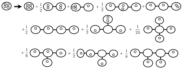
Figure 1: The modular transformation of $F_{4}^{\rm NS}$.

Moreover the weight $1/s$ of each graph is obtained simply by counting the multiplicity of each surface inside the graph as in the unrefined case. This is shown for instance on Fig. 1 for $F_{4}^{\rm NS}$.

Let us look at some concrete examples. Starting from (2.22), one can show that

$$\partial F_{0}\to A\partial F_{0}+B\epsilon^{(0)},$$ (4.68)

$$\partial F_{1}^{\rm NS}\to\left(C\tau+D\right)^{-1}\partial F_{1}^{\rm NS},$$

$$\partial F_{2}^{\rm NS}\to\left(C\tau+D\right)^{-1}\left(\partial F_{2}^{\rm NS}+{\mathcal{K}}\partial F_{1}^{\rm NS}\partial^{2}F_{1}^{\rm NS}\right.$$

$$\qquad\qquad\qquad\qquad\quad\qquad\left.+{1\over 2}\partial^{3}F_{0}\left(\partial F_{1}^{\rm NS}\right)^{2}{\mathcal{K}}^{2}\right),$$

where we used that $\partial^{3}F_{0}$ behaves as a weak Jacobi form of weight -3 under (2.12) as shown for instance in abk . By integrating (4.68) we obtain that $F_{1}^{\rm NS}$ is modular invariant while

$$F_{2}^{\rm NS}\to F_{2}^{\rm NS}+{1\over 2}{\mathcal{K}}\left(\partial F_{1}^{\rm NS}\right)^{2}.$$ (4.69)

Similarly one can show that

$$F_{3}^{\rm NS} \to F_{3}^{\rm NS}+\frac{1}{6}{\mathcal{K}}^{3}\partial^{3}F_{0}(\partial F_{1}^{\rm NS})^{3}+{\mathcal{K}}\partial F_{1}^{\rm NS}\partial F_{2}^{\rm NS}+\frac{1}{2}{\mathcal{K}}^{2}(\partial F_{1}^{\rm NS})^{2}\partial^{2}F_{1}^{\rm NS},$$ (4.70)

$$F_{4}^{\rm NS} \to F_{4}^{\rm NS}+\frac{1}{2}{\mathcal{K}}(\partial F_{2}^{\rm NS})^{2}+{\mathcal{K}}\partial F_{1}^{\rm NS}\partial F_{3}^{\rm NS}+\frac{1}{2}{\mathcal{K}}^{2}(\partial F_{1}^{\rm NS})^{2}\partial^{2}F_{2}^{\rm NS}+{\mathcal{K}}^{2}\partial F_{1}^{\rm NS}\partial^{2}F_{1}^{\rm NS}\partial F_{2}^{\rm NS}$$

$$+\frac{1}{2}{\mathcal{K}}^{3}(\partial F_{1}^{\rm NS})^{2}(\partial^{2}F_{1}^{\rm NS})^{2}+\frac{1}{6}{\mathcal{K}}^{3}\partial^{3}F_{1}^{\rm NS}(\partial F_{1}^{\rm NS})^{3}+\frac{1}{24}{\mathcal{K}}^{4}\partial^{4}F_{0}^{\rm NS}(\partial F_{1}^{\rm NS})^{4}$$

$$+\frac{1}{2}{\mathcal{K}}^{3}\partial^{3}F_{0}^{\rm NS}(\partial F_{1}^{\rm NS})^{2}\partial F_{2}^{\rm NS}+\frac{1}{2}{\mathcal{K}}^{4}\partial^{3}F_{0}(\partial F_{1}^{\rm NS})^{3}\partial^{2}F_{1}^{\rm NS}+\frac{1}{8}{\mathcal{K}}^{5}\partial^{3}F_{0}^{2}(\partial F_{1}^{\rm NS})^{4},$$

$$F_{5}^{\rm NS}\to F_{5}^{\rm NS}+\frac{1}{2}\mathcal{K}^{2}\partial^{2}F_{1}^{\rm NS}\left(\partial F_{2}^{\rm NS}\right)^{2}+\mathcal{K}\partial F_{1}^{\rm NS}\partial F_{4}^{\rm NS}+\mathcal{K}^{3}\partial F_{1}^{\rm NS}\left(\partial^{2}F_{1}^{\rm NS}\right)^{2}\partial F_{2}^{\rm NS}$$ (4.71)

$$+\mathcal{K}^{2}\partial F_{1}^{\rm NS}\partial^{2}F_{1}^{\rm NS}\ \partial F_{3}^{\rm NS}+\mathcal{K}\partial F_{2}^{\rm NS}\partial F_{3}^{\rm NS}$$

$$+\frac{1}{2}\mathcal{K}^{3}\partial^{3}F_{0}\partial F_{1}^{\rm NS}\left(\partial F_{2}^{\rm NS}\right)^{2}+\mathcal{K}^{2}\partial F_{1}^{\rm NS}\partial F_{2}^{\rm NS}\partial^{2}F_{2}^{\rm NS}+\frac{1}{2}\mathcal{K}^{2}\left(\partial F_{1}^{\rm NS}\right)^{2}\partial^{2}F_{3}^{\rm NS}$$

$$+\mathcal{K}^{3}\left(\partial F_{1}^{\rm NS}\right)^{2}\partial^{2}F_{1}^{\rm NS}\partial^{2}F_{2}^{\rm NS}+\frac{1}{2}\mathcal{K}^{4}\left(\partial F_{1}^{\rm NS}\right)^{2}\left(\partial^{2}F_{1}^{\rm NS}\right)^{3}+\frac{1}{2}\mathcal{K}^{4}\partial^{3}F_{0}\left(\partial F_{1}^{\rm NS}\right)^{3}\partial^{2}F_{2}^{\rm NS}$$

$$+\frac{1}{2}\mathcal{K}^{3}\partial^{3}F_{0}\left(\partial F_{1}^{\rm NS}\right)^{2}\ \partial F_{3}^{\rm NS}+\frac{3}{2}\mathcal{K}^{4}\partial^{3}F_{0}\left(\partial F_{1}^{\rm NS}\right)^{2}\partial^{2}F_{1}^{\rm NS}\partial F_{2}^{\rm NS}$$

$$+\mathcal{K}^{5}\partial^{3}F_{0}\left(\partial F_{1}^{\rm NS}\right)^{3}\left(\partial^{2}F_{1}^{\rm NS}\right)^{2}+\frac{1}{2}\mathcal{K}^{5}\partial^{3}F_{0}^{2}\left(\partial F_{1}^{\rm NS}\right)^{3}\partial F_{2}^{\rm NS}$$

$$+\frac{1}{8}\mathcal{K}^{7}\partial^{3}F_{0}^{3}\left(\partial F_{1}^{\rm NS}\right)^{5}+\frac{5}{8}\mathcal{K}^{6}\partial^{3}F_{0}^{2}\left(\partial F_{1}^{\rm NS}\right)^{4}\partial^{2}F_{1}^{\rm NS}+\frac{1}{2}\mathcal{K}^{3}\partial^{3}F_{1}^{\rm NS}\left(\partial F_{1}^{\rm NS}\right)^{2}\partial F_{2}^{\rm NS}$$

$$+\frac{1}{6}\mathcal{K}^{4}\partial^{4}F_{0}^{\rm NS}\left(\partial F_{1}^{\rm NS}\right)^{3}\partial F_{2}^{\rm NS}+\frac{1}{4}\mathcal{K}^{5}\partial^{3}F_{0}\partial^{3}F_{1}^{\rm NS}\left(\partial F_{1}^{\rm NS}\right)^{4}+\frac{1}{6}\mathcal{K}^{3}\partial^{3}F_{2}^{\rm NS}\left(\partial F_{1}^{\rm NS}\right)^{3}$$

$$+\frac{1}{2}\mathcal{K}^{4}\partial^{3}F_{1}^{\rm NS}\left(\partial F_{1}^{\rm NS}\right)^{3}\partial^{2}F_{1}^{\rm NS}+\frac{1}{120}\mathcal{K}^{5}\partial^{5}F_{0}^{\rm NS}\left(\partial F_{1}^{\rm NS}\right)^{5}+\frac{1}{6}\mathcal{K}^{5}\partial^{4}F_{0}^{\rm NS}\left(\partial F_{1}^{\rm NS}\right)^{4}\partial^{2}F_{1}^{\rm NS}$$

$$+\frac{1}{12}\mathcal{K}^{6}\partial^{3}F_{0}\partial^{4}F_{0}\left(\partial F_{1}^{\rm NS}\right)^{5}+\frac{1}{24}\mathcal{K}^{4}\partial^{4}F_{1}^{\rm NS}\left(\partial F_{1}^{\rm NS}\right)^{4}.$$

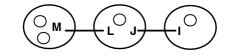
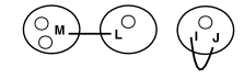
Figure 2: A graphical representation of (4.73) (top), and of (4.74) (bottom).

The above transformations have been worked out by an explicit computation from (2.22), however it is easy to check that they can be derived by using the diagrammatic rules explained around equation (4.66). Similarly we have explicitly check these diagrammatic rules also for higher $F_{g}$.

The structure of the indices in (4.70) and (4.71) is always such that the corresponding diagram is connected. For instance let us consider the term

$${\mathcal{K}}^{2}\partial F_{1}^{\rm NS}\partial^{2}F_{1}^{\rm NS}\partial F_{2}^{\rm NS}$$ (4.72)

appearing in the modular transformation of $F_{4}$ in (4.70). The correct structure of the indices is

$${\mathcal{K}}_{IJ}{\mathcal{K}}_{LM}\partial_{I}F_{1}^{\rm NS}\partial_{J}\partial_{L}F_{1}^{\rm NS}\partial_{M}F_{2}^{\rm NS}.$$ (4.73)

This is represented by the diagram in the top of Fig. 2. As an example let us consider the following index structure

$${\mathcal{K}}_{IJ}{\mathcal{K}}_{LM}\partial_{L}F_{1}^{\rm NS}\partial_{J}\partial_{I}F_{1}^{\rm NS}\partial_{M}F_{2}^{\rm NS}.$$ (4.74)

This is represented by the diagram in the bottom of Fig. 2. This diagram is disconnected, and (4.74) has indeed the wrong index structure. It could be that there are two ”connected” index structures for a single term. This is the case for instance for the term

$${5\over 24}{\mathcal{K}}^{3}\partial^{3}\widehat{F}_{0}^{2}$$ (4.75)

appearing in the modular transformation of $F_{2}$ (B.170). In this case one has to consider all the connected index structures with the corresponding symmetry factor. For instance (4.75) reads

$${1\over 12}{\mathcal{K}}_{IJ}{\mathcal{K}}_{LM}{\mathcal{K}}_{PQ}\partial_{I}\partial_{L}\partial_{P}\widehat{F}_{0}\partial_{J}\partial_{M}\partial_{Q}\widehat{F}_{0}+$$ (4.76)

$${1\over 8}{\mathcal{K}}_{IJ}{\mathcal{K}}_{LM}{\mathcal{K}}_{PQ}\partial_{I}\partial_{J}\partial_{P}\widehat{F}_{0}\partial_{L}\partial_{M}\partial_{Q}\widehat{F}_{0}.$$

4.2 The quantum Kähler parameters

Figure 3: The modular transformation of $\epsilon^{(4)}$. The blue dashed surfaces represent the $n$ ”satellites” and the red ones represent $\partial^{n+1}F_{g}^{\rm NS}$

Likewise, we notice that the transformation properties of the ${\rm n}^{\rm th}$ component of the A period, $\epsilon^{(n)}$, can be encoded by using diagrammatic rules. By doing an explicit computation one can show that (2.22) leads to

$$\epsilon^{(0)}\to C\partial F_{0}+D\epsilon^{(0)},$$ (4.77)

$$\epsilon^{(1)}\to C\left(\partial F_{1}^{\rm NS}+\epsilon^{(1)}\tau\right)+D\epsilon^{(1)},$$

$$\epsilon^{(2)}\to C\left(\partial F_{2}^{\rm NS}+\epsilon^{(1)}\partial^{2}F_{1}^{\rm NS}+{1\over 2}(\epsilon^{(1)})^{2}\partial^{3}F_{0}+\epsilon^{(2)}\tau\right)+D\epsilon^{(2)},$$

$$\epsilon^{(3)}\to D\epsilon^{(3)}+C\left(\frac{1}{6}(\epsilon^{(1)})^{3}\partial^{4}F_{0}+\epsilon^{(1)}\epsilon^{(2)}\partial^{3}F_{0}\right.$$

$$\qquad\quad\left.+\epsilon^{(3)}\partial^{2}F_{0}+\frac{1}{2}(\epsilon^{(1)})^{2}\partial^{3}F_{1}^{\rm NS}+\epsilon^{(2)}\ \partial^{2}F_{1}^{\rm NS}+\epsilon^{(1)}\partial^{2}F_{2}^{\rm NS}+\partial F_{3}^{\rm NS}\right),$$

$$\epsilon^{(4)}\to D\epsilon^{(4)}+C\left(\partial F_{4}^{\rm NS}+\epsilon^{(4)}\partial^{2}F_{0}+\epsilon^{(3)}\partial^{2}F_{1}^{\rm NS}+\epsilon^{(2)}\partial^{2}F_{2}^{\rm NS}+\epsilon^{(1)}\partial^{2}F_{3}^{\rm NS}+{1\over 2}(\epsilon^{(2)})^{2}\partial^{3}F_{0}\right.$$

$$\qquad\quad\epsilon^{(1)}\epsilon^{(3)}\partial^{3}F_{0}+\epsilon^{(1)}\epsilon^{(2)}\partial^{3}F_{1}^{\rm NS}+{1\over 2}(\epsilon^{(1)})^{2}\partial^{3}F_{2}^{\rm NS}+{1\over 2}(\epsilon^{(1)})^{2}\epsilon^{(2)}\partial^{4}F_{0}+{1\over 6}(\epsilon^{(1)})^{3}\partial^{4}F_{1}^{\rm NS}$$

$$\qquad\quad\left.+{1\over 24}(\epsilon^{(1)})^{4}\partial^{5}F_{0}\right).$$

We encode the above transformation by saying that

$$\epsilon^{(k)}\to\left(D+C\tau\right)\epsilon^{(k)}+C\mathcal{G}(k),$$ (4.78)

where $\mathcal{G}(k)$ can be represented as a sum of diagrams. Each of these diagrams is made of one Riemann surface of genus $g$ with one leg sticking out and $n\geq 0$ ”satellites” of genus $k>g_{i}\geq 1$ ( representing $\epsilon^{(g_{i})}$ ) such that

$$\sum_{i=1}^{n}g_{i}+g=k.$$ (4.79)

This is shown on Fig. 3 for $k=4$. The multiplicity is computed in the standard way.

In appendix A we check by an explicit computation the rules (4.77) in the case of the local ${\mathbb{P}}^{2}$ geometry. The comparison between our results (4.77) and the direct computation leads to interesting identities, as for instance (A.154),(A.157), (A.158), which can be checked explicitly.

4.3 The wave function and the holomorphic anomaly

We observe that the diagrammatic rules described in section (4.1) can be encoded in some kind of wave function behavior similar to the one for the standard free energies emo ; abk . Let us define emo

$$\hbar^{2}S(\epsilon,\eta,\hbar,\mathcal{K})=-{1\over 2}(\eta-\epsilon){\mathcal{K}}^{-1}(\eta-\epsilon)-(\eta-\epsilon)\partial_{\epsilon}F_{0}(\epsilon)-{1\over 2}(\eta-\epsilon)\partial_{\epsilon}^{2}F_{0}(\epsilon)(\eta-\epsilon),$$ (4.80)

where ${\mathcal{K}}$ is defined in (4.67) and $\epsilon$ denotes here the classical period (2.11). Then the previous transformation rules can be written as

$${\rm e}^{\hbar^{-1}F^{\rm NS}(\hbar,\epsilon,{\mathcal{K}})}=\left({1\over\hbar\sqrt{2\pi\det{\mathcal{K}}}}\int{\rm d}\eta{\rm e}^{S(\epsilon,\eta,\hbar,\mathcal{K})+\hbar^{-1}{F}^{\rm NS}(\hbar,\eta)}\right)\Big{|}_{g~{}\rm{fixed}},$$ (4.81)

where by $\mid_{g~{}\rm{fixed}}$ we mean that at each order in the $\hbar^{2g-2}$ expansion we keep only diagrams with total genus $g$. We use $F^{\rm NS}(\hbar,\epsilon,{\mathcal{K}})$ to note the NS free energy obtained after performing the modular transformation (2.12). When ${\mathcal{K}}=0$ we simply note $F^{\rm NS}(\hbar,\epsilon)$. To implement the constraint $\mid_{g~{}\rm{fixed}}$, it is useful to introduce an extra variable $y$ and consider

$$Z_{y}(\mathcal{K})=\left({1\over\hbar\sqrt{2\pi\det{\mathcal{K}}}}\int{\rm d}\eta{\rm e}^{y^{-1}S(\epsilon,\eta,\hbar,\mathcal{K})+y^{-1}\hbar^{-1}{F}^{\rm NS}(\hbar,\eta)}\right).$$ (4.82)

The transformations rules for the $F_{g}^{\rm NS}$’s can then be computed by doing a saddle point analysis of the integral appearing on the r.h.s. of (4.81) or (4.82) . It is easy to see that the saddle point for small $\hbar$ is given by

$$\eta=\epsilon.$$ (4.83)

We explicitly checked that the saddle point analysis of (4.81) agrees with (4.69), (4.70), (4.71) which have been at first derived from (2.22). When we compute the saddle point of (4.82), at each order in the $\hbar^{2g-2}$ expansion, the diagrams with total genus $g$ are multiplied by a factor of $y^{-1}$. Similarly the diagrams with total genus $g^{\prime}<g$ are multiplied by a positive power of $y$. For instance at order $\hbar^{2}$ the saddle point of (4.82) gives

$$S_{2}(\mathcal{K},y)=y^{-1}F_{2}^{\rm NS}+y^{-1}\frac{1}{2}{\mathcal{K}}(\partial F_{1}^{\rm NS})^{2}+\frac{1}{2}{\mathcal{K}}\partial^{2}F_{1}^{\rm NS}+y\frac{1}{8}{\mathcal{K}}^{2}\partial^{4}F_{0}+\frac{1}{2}{\mathcal{K}}^{2}\partial^{3}F_{0}\partial F_{1}^{\rm NS}+y\frac{5}{24}{\mathcal{K}}^{3}\partial^{3}F_{0}^{2}.$$ (4.84)

It follows that

$$F_{2}^{\rm NS}(\epsilon,\mathcal{K})=\lim_{y\to 0}{y}S_{2}(\mathcal{K},y)=F_{2}^{\rm NS}+\frac{1}{2}\mathcal{K}(\partial F_{1}^{\rm NS})^{2}.$$ (4.85)

Therefore we have a systematic way to compute the l.h.s. of (4.81) as:

$$\sum_{g\geq 0}\hbar^{2g-2}F^{\rm NS}_{g}(\epsilon,\mathcal{K})=\lim_{y\to 0}y\log Z_{y}(\mathcal{K}).$$ (4.86)

Notice that if we set $y=1$ we recover the wave function behavior of the standard topological string free energy abk ; emo .

By following emo , one can derive from (4.82) the holomorphic anomaly equation for the NS free energies and check that it reproduce the well known result hk ; hkpk ; huangNS . Let us introduce a non–holomorphic dependence in $\overline{\epsilon}_{I}$ by setting emo

$$\mathcal{K}_{0}=\left(\overline{\tau}-\tau\right)^{-1}$$ (4.87)

and define

$$Z= \left({1\over\hbar\sqrt{2\pi}}\int{\rm d}\eta{\rm e}^{y^{-1}S(\epsilon,\eta,\hbar,\mathcal{K}_{0})+y^{-1}\hbar^{-1}{F}^{\rm NS}(\hbar,\eta)}\right),$$ (4.88)

$$\tilde{Z}= \left({1\over\hbar\sqrt{2\pi\det{\mathcal{K}}_{0}}}\int{\rm d}\eta{\rm e}^{y^{-1}S(\epsilon,\eta,\hbar,\mathcal{K}_{0})+y^{-1}\hbar^{-1}{F}^{\rm NS}(\hbar,\eta)}\right){\rm e}^{-y^{-1}\hbar^{-2}F_{0}(\epsilon)-y^{-1}F_{1}^{\rm NS}(\epsilon)},$$

$$\widehat{Z}= \left({1\over\hbar\sqrt{2\pi}}\int{\rm d}\eta{\rm e}^{y^{-1}S(\epsilon,\eta,\hbar,\mathcal{K}_{0})+y^{-1}\hbar^{-1}{F}^{\rm NS}(\hbar,\eta)}\right){\rm e}^{-y^{-1}\hbar^{-2}F_{0}(\epsilon)}.$$

Then we have

$${1\over\tilde{Z}}\partial_{\overline{K}}\tilde{Z}={1\over 2}\left(\mathcal{K}_{0}^{IJ}\partial_{\overline{K}}\overline{\tau}_{IJ}-y^{-1}\hbar^{-2}\langle(\eta-\epsilon)^{I}(\eta-\epsilon)^{J}\rangle\partial_{\overline{K}}\overline{\tau}_{IJ}\right)$$ (4.89)

where $\langle\cdot\rangle$ denotes the expectation value w.r.t. the integral in the first line of (4.88). Similarly one has

$${1\over\widehat{Z}}\partial_{I}\widehat{Z}= y^{-1}\hbar^{-2}\langle\left(\overline{\tau}-\tau\right)_{IJ}(\eta-\epsilon)^{J}\rangle,$$ (4.90)

$${1\over\widehat{Z}}\partial_{I}\partial_{J}\widehat{Z}= -\hbar^{-2}y^{-1}\left(\overline{\tau}-\tau\right)_{IJ}+\hbar^{-4}y^{-2}\left(\overline{\tau}-\tau\right)_{IM}\left(\overline{\tau}-\tau\right)_{JL}\langle(\eta-\epsilon)^{M}(\eta-\epsilon)^{L}\rangle$$

$$-\hbar^{-2}y^{-1}\partial_{I}\tau_{JM}\langle(\eta-\epsilon)^{M}\rangle.$$

In particular

$$y\partial_{\overline{K}}\log\tilde{Z}={y\over 2}\hbar^{2}\overline{C}^{IJ}_{\overline{K}}\left(y\partial_{I}\partial_{J}\log\widehat{Z}+y\partial_{I}\log\widehat{Z}\partial_{J}\log\widehat{Z}+y\mathcal{K}_{0}^{LM}\partial_{I}\tau_{JM}\partial_{L}\log\widehat{Z}\right),$$ (4.91)

where

$$\overline{C}^{IJ}_{\overline{K}}=-{\mathcal{K}}_{0}^{IM}{\partial^{3}\overline{F}_{0}\over\partial\overline{\epsilon}_{N}\partial\overline{\epsilon}_{M}\partial\overline{\epsilon}_{K}}{\mathcal{K}}_{0}^{NJ}.$$ (4.92)

When $y=1$ (4.91) takes the form of the holomorphic anomaly equation of unrefined topological strings bcov ; emo . If instead we take $y\to 0$ in (4.91), by using (4.86), we recover the refined holomorphic anomaly equation for the NS free energies hk ; hkpk ; huangNS

$$\partial_{\overline{I}}F^{\rm NS}_{g}={1\over 2}\overline{C}^{JK}_{\overline{I}}\sum_{h\geq 1}\partial_{J}F_{n}^{\rm NS}\partial_{K}F_{g-n}^{\rm NS},\quad g>1.$$ (4.93)

5 Symplectic invariance and the spectral determinant

We are now going to use the results of section 4 to investigate the modular properties of the spectral determinant (3.41). As explained previously the strategy is to expand the spectral determinant around $\hbar=2\pi$:

$$\Xi({\boldsymbol{\kappa}},\hbar)=\sum_{n\geq 0}{1\over n!}{{\rm d}^{n}\Xi({\boldsymbol{\kappa}},2\pi)\over{\rm d}^{n}\hbar}(\hbar-2\pi)^{n},$$ (5.94)

where the leading order $n=0$ is given by (3.49). We find that the $n^{\rm th}$ order in this expansion can be written in closed form in terms of $F_{g}$, $F_{h}^{\rm NS}$ with $g,h\leq n$ and derivatives of the theta function (3.51). In the following we work out the first few orders in the expansion (5.94) and we show modular invariance by and explicit computation. We will then argue that this is the case at each order in the $\hbar-2\pi$ expansion. This is done by using the combinatorial techniques developed in em together with the rules worked out in section 4.

We use the shortcut notation

$$\Theta=\Theta_{0,\beta}(\widehat{\boldsymbol{\xi}},\widehat{\tau}),$$ (5.95)

together with

$$\left(\partial_{2\pi{\rm i}{\boldsymbol{\xi}}}-{1\over(2\pi{\rm i})}{\boldsymbol{T}}\right)^{n}\Theta=\left(\prod_{I=1}^{n}\left(\partial_{2\pi{\rm i}{\xi_{p_{I}}}}-{1\over(2\pi{\rm i})}{T_{p_{I}}}\right)\right)\Theta=\Theta^{(n)}.$$ (5.96)

The modular properties of $\Theta^{(n)}$ have been worked out in em and they can be schematically represented as

$${\Theta^{(n)}\over\Theta}\to(C\widehat{\tau}+D)^{n}\sum_{j=0}^{[n/2]}(2j-1)!!\binom{n}{2j}\left(-{{\mathcal{K}}\over 2\pi{\rm i}}\right)^{j}{\Theta^{(n-2j)}\over\Theta},$$ (5.97)

where ${\mathcal{K}}$ is given in (3.56). Notice that when we refer to modular invariance we always mean up to a change of characteristic in the theta function (3.52) as in em . In the following we will omit the constant map contribution $A(\hbar)$ appearing in the spectral determinant (3.33) since it clearly does not affect the modular properties. To be more concrete we will do the analysis in the case of a mirror curve with genus one.

5.1 First order

Let us look at the first order in the $\hbar-2\pi$ expansion. After some computations we find

$$\partial_{\hbar}J(\mu+2\pi{\rm i}n,\hbar)\Big{|}_{\hbar=2\pi}= \left(n-{\widehat{T}\over 2\pi{\rm i}}\right)\left({\rm i}\partial_{T}\widehat{F}_{1}+{\rm i}\partial_{T}\widehat{F}_{1}^{\rm NS}\right)+\frac{1}{6}{\rm i}\partial^{3}_{T}\widehat{F}_{0}\left(n-{\widehat{T}\over 2\pi{\rm i}}\right)^{3}.$$ (5.98)

It follows that

$${{\rm d}\over{\rm d}\hbar}\Xi(\kappa,\hbar)\Big{|}_{\hbar=2\pi} ={\rm e}^{N^{2}{\widehat{F}_{0}}+\widehat{F}_{1}-\widehat{F}_{1}^{\rm NS}}\Big{(}{{\rm i}\over 6}\partial_{T}^{3}{\widehat{F}_{0}}\Theta^{(3)}+{\rm i}\left(\partial_{T}\widehat{F}_{1}+\partial_{T}\widehat{F}_{1}^{\rm NS}\right)\Theta^{(1)}\Big{)},$$ (5.99)

where we used $\partial_{\hbar}T\mid_{\hbar=2\pi}=0$. By using the modular properties of the unrefined free energy abk ; em , together with (5.97) we have

$$\partial_{T}^{3}{\widehat{F}_{0}}\to {1\over(C\widehat{\tau}+D)^{3}}\partial_{T}^{3}{\widehat{F}_{0}},$$ (5.100)

$$\partial_{T}\widehat{F}_{1}\to (C\widehat{\tau}+D)^{-1}\left(\partial_{T}\widehat{F}_{1}+{1\over 2}{{\mathcal{K}}\over 2\pi{\rm i}}\partial_{T}^{3}{\widehat{F}_{0}}\right),$$

$${\Theta\over\Theta}^{(1)}\to (C\widehat{\tau}+D){\Theta\over\Theta}^{(1)},$$

$${\Theta\over\Theta}^{(3)}\to (C\widehat{\tau}+D)^{3}\left({\Theta\over\Theta}^{(3)}-{3}{{\mathcal{K}}\over 2\pi{\rm i}}{\Theta\over\Theta}^{(1)}\right).$$

From the invariance of $F_{1}^{\rm NS}$ it follows that

$$\partial_{T}\widehat{F}_{1}^{\rm NS}\to\left(C\widehat{\tau}+D\right)^{-1}\partial_{T}\widehat{F}_{1}^{\rm NS}.$$ (5.101)

Therefore (5.99) is manifestly modular invariant as expected.

5.2 Second order

At the second order we have

$${d^{2}\over d\hbar^{2}}\Xi(\kappa,\hbar)\Big{|}_{\hbar=2\pi}=\sum_{n} \left(\partial_{\hbar}^{2}J(\mu+2\pi{\rm i}n,\hbar)+\left(\partial_{\hbar}J(\mu+2\pi{\rm i}n,\hbar)\right)^{2}+\partial_{\hbar}^{2}T\partial_{T}J(\mu+2\pi{\rm i}n,\hbar)\right)\Big{|}_{\hbar=2\pi}$$ (5.102)

$$\times{\rm e}^{J(\mu+2\pi{\rm i}n,2\pi)}$$

One can show from (3.33) that

$$\partial_{\hbar}^{2}J(\mu+2\pi{\rm i}n,\hbar)\big{|}_{\hbar=2\pi}= -\frac{1}{12}\left(n-{\widehat{T}\over 2\pi{\rm i}}\right)^{4}\partial_{T}^{4}\widehat{F}_{0}-\frac{{\rm i}\left(n-{\widehat{T}\over 2\pi{\rm i}}\right)^{3}\partial_{T}^{3}\widehat{F}_{0}}{6\pi}$$ (5.103)

$$-\left(n-{\widehat{T}\over 2\pi{\rm i}}\right)^{2}\partial_{T}^{2}\widehat{F}_{1}-{{\rm i}\over\pi}\left(n-{\widehat{T}\over 2\pi{\rm i}}\right)\partial_{T}\widehat{F}_{1}$$

$$-2\widehat{F}_{2}-{6}\widehat{F}_{2}^{\rm NS}.$$

Similarly

$$\partial_{\hbar}^{2}T\partial_{T}J(\mu+2\pi{\rm i}n,\hbar)\big{|}_{\hbar=2\pi}=2\widehat{T}^{(1)}\left(\partial_{T}\widehat{F}_{1}-\partial_{T}\widehat{F}_{1}^{\rm NS}+{1\over 2}\partial_{T}^{3}\widehat{F}_{0}(n-{\widehat{T}\over 2\pi{\rm i}})^{2}\right),$$ (5.104)

where we use that

$$\partial_{\hbar}^{2}T\mid_{\hbar=2\pi}(z)=\partial_{\hbar}^{2}T\mid_{\hbar=0}((-1)^{B}z)=2\widehat{T}^{(1)},$$ (5.105)

and $B$ is the $B$ field. It follows that

$${1\over 2}{d^{2}\over d\hbar^{2}}\Xi(\kappa,\hbar)\Big{|}_{\hbar=2\pi}= {\rm e}^{N^{2}{\widehat{F}_{0}}+\widehat{F}_{1}-\widehat{F}_{1}^{\rm NS}}\Big{(}\left(-\widehat{F}_{2}-3\widehat{F}_{2}^{\rm NS}\right)\Theta-{1\over 72}\left(\partial_{T}^{3}{\widehat{F}_{0}}\right)^{2}\Theta^{(6)}-{1\over 24}\partial_{T}^{4}{\widehat{F}_{0}}\Theta^{(4)}$$ (5.106)

$$-{1\over 6}\partial_{T}^{3}{\widehat{F}_{0}}\left(\partial_{T}\widehat{F}_{1}+\partial_{T}\widehat{F}_{1}^{\rm NS}\right)\Theta^{(4)}-{{\rm i}\over 2\pi}\left({1\over 6}\partial_{T}^{3}{\widehat{F}_{0}}\Theta^{(3)}+\partial_{T}{\widehat{F}_{0}}\Theta^{(1)}\right)$$

$$-{1\over 2}\left((\partial_{T}\widehat{F}_{1}+\partial_{T}\widehat{F}_{1}^{\rm NS})^{2}+\partial_{T}^{2}\widehat{F}_{1}\right)\Theta^{(2)}$$

$$+\widehat{T}^{(1)}\left(\partial_{T}\widehat{F}_{1}\Theta-\partial_{T}\widehat{F}_{1}^{\rm NS}\Theta+{1\over 2}\partial_{T}^{3}{\widehat{F}_{0}}\Theta^{(2)}\right)\Big{)}.$$

When the NS quantities are set to zero, modular invariance of (5.106) is straightforward from em . Therefore it is enough to show that the following term is invariant under (2.12):

$${\rm e}^{N^{2}{\widehat{F}_{0}}+\widehat{F}_{1}-\widehat{F}_{1}^{\rm NS}} \Big{(}-3\widehat{F}_{2}^{\rm NS}\Theta-{1\over 6}\partial_{T}^{3}{\widehat{F}_{0}}\partial_{T}\widehat{F}_{1}^{\rm NS}\ \Theta^{(4)}-{1\over 2}\left(\left(\partial_{T}\widehat{F}_{1}^{\rm NS}\right)^{2}+2\partial_{T}\widehat{F}_{1}^{\rm NS}\partial_{T}\widehat{F}_{1}\right)\Theta^{(2)}$$ (5.107)

$$+\widehat{T}^{(1)}\left(\partial_{T}\widehat{F}_{1}\Theta^{(0)}-\partial_{T}\widehat{F}_{1}^{\rm NS}\Theta^{(0)}+{1\over 2}\partial_{T}^{3}{\widehat{F}_{0}}\Theta^{(2)}\right)\Big{)}.$$

By using the transformation properties of the standard free energy abk ; em ; emo together with (4.68) and (5.97) we find

$${1\over 6}\partial_{T}^{3}{\widehat{F}_{0}}\left(\partial_{T}\widehat{F}_{1}^{\rm NS}\right)\Theta^{(4)}/\Theta\to\partial_{T}^{3}{\widehat{F}_{0}}\left(\partial_{T}\widehat{F}_{1}^{\rm NS}\right)\left({1\over 6}{\Theta\over\Theta}^{(4)}-{{\mathcal{K}}\over 2\pi{\rm i}}{\Theta\over\Theta}^{(2)}+{1\over 2}\left({{\mathcal{K}}\over 2\pi{\rm i}}\right)^{2}\right).$$ (5.108)

Similarly

$$\partial_{T}\widehat{F}_{1}^{\rm NS}\partial_{T}\widehat{F}_{1}\Theta^{(2)}/\Theta\to \partial_{T}\widehat{F}_{1}^{\rm NS}\partial_{T}\widehat{F}_{1}\left({\Theta\over\Theta}^{(2)}-{{\mathcal{K}}\over 2\pi{\rm i}}\right)$$ (5.109)

$$+{1\over 2}{{\mathcal{K}}\over 2\pi{\rm i}}\partial_{T}\widehat{F}_{1}^{\rm NS}\partial_{T}^{3}\widehat{F}_{0}\left({\Theta\over\Theta}^{(2)}-{{\mathcal{K}}\over 2\pi{\rm i}}\right).$$

Moreover

$$-{1\over 2}\left(\partial_{T}\widehat{F}_{1}^{\rm NS}\right)^{2}\Theta^{(2)}/\Theta\to-\left(\partial_{T}\widehat{F}_{1}^{\rm NS}\right)^{2}\left({1\over 2}{\Theta\over\Theta}^{(2)}-{1\over 2}{{\mathcal{K}}\over 2\pi{\rm i}}\right),$$ (5.110)

and

$$3\widehat{F}_{2}^{\rm NS}\to 3\widehat{F}_{2}^{\rm NS}+3{{\mathcal{K}}\over 2}\left({1\over(2\pi{\rm i})^{1/2}}\partial_{T}\widehat{F}_{1}^{\rm NS}\right)^{2}.$$ (5.111)

By summing up (5.108),(5.109),(5.110) and (5.111) we obtain modular invariance up to an additional term given by

$${{\mathcal{K}}\over 2\pi{\rm i}}\partial_{T}\widehat{F}_{1}^{\rm NS}\left(-\partial_{T}\widehat{F}_{1}^{\rm NS}+\partial_{T}\widehat{F}_{1}\right)+{1\over 2}{{\mathcal{K}}\over 2\pi{\rm i}}\partial_{T}\widehat{F}_{1}^{\rm NS}\partial_{T}^{3}\widehat{F}_{0}{\Theta\over\Theta}^{(2)}.$$ (5.112)

For the last term in (5.107) we have

$$\widehat{T}^{(1)}\left(\partial_{T}\widehat{F}_{1}+\partial_{T}\widehat{F}_{1}^{\rm NS}+{1\over 2}\partial_{T}^{3}{\widehat{F}_{0}}{\Theta\over\Theta}^{(2)}\right)\to \widehat{T}^{(1)}\left(\partial_{T}\widehat{F}_{1}-\partial_{T}\widehat{F}_{1}^{\rm NS}+{1\over 2}\partial_{T}^{3}{\widehat{F}_{0}}{\Theta\over\Theta}^{(2)}\right)$$ (5.113)

$$-\partial_{T}\widehat{F}_{1}^{\rm NS}{{\mathcal{K}}\over 2\pi{\rm i}}\left({1\over 2}\partial_{T}^{3}\widehat{F}_{0}{\Theta\over\Theta}^{(2)}+\partial_{T}\widehat{F}_{1}-\partial_{T}\widehat{F}_{1}^{\rm NS}\right).$$

In particular the second term in (5.113) precisely cancels the one in (5.112). Hence modular invariance is manifest also at the second order.

5.3 The general mechanism

The general structure of the $n^{\rm th}>0$ order term in the expansion (5.94) is the following. There is a part which involves only standard topological strings

$$\Xi(\kappa,2\pi)\prod_{i}^{k}\partial^{n_{i}}_{T}\widehat{F}_{g_{i}}\Theta^{(n_{1}+\cdots+n_{k})}/\Theta,\qquad g_{i}\leq n.$$ (5.114)

By using the combinatorial rules of em it follows that this part is modular invariant. However we also have two other contributions of the form ($g_{i},g_{j}<n$)

$$\Xi(\kappa,2\pi)\prod_{i}^{k}\partial^{n_{i}}_{T}\widehat{F}_{g_{i}}\prod_{j}^{\ell}\partial^{m_{j}}_{T}\widehat{F}_{g_{j}}^{\rm NS}\Theta^{(n_{1}+m_{1}+\cdots+m_{\ell}+n_{k})}/\Theta,$$ (5.115)

$$\Xi(\kappa,2\pi)\prod_{p}^{s}\widehat{T}^{(r_{p})}\prod_{i}^{k}\partial^{n_{i}}_{T}\widehat{F}_{g_{i}}\prod_{j}^{\ell}\partial^{m_{j}}_{T}\widehat{F}_{g_{j}}^{\rm NS}\Theta^{(n_{1}+m_{1}\cdots+m_{\ell}+n_{k}-s)}/\Theta.$$ (5.116)

Let us look at the first term (5.115). Since the number of derivatives acting on $\Theta$ is the same as acting on the free energy, when we apply a symplectic transformation we recover the same term plus an extra factor. The same happens also for the second term (5.116). Indeed $\widehat{T}^{(k)}$ get a multiplicative factor of $(C\widehat{\tau}+D)$ under modular transformations as explained in section 4.2. Notice that (5.116) appears when we consider the $\hbar$ dependence of $T$.

None of the terms (5.115) and (5.116) is modular invariant: they both transform into itself plus an additional factor. At each order in the $\hbar-2\pi$ expansion, the extra factor coming from (5.115) cancels the one coming from (5.116). Although we don’t have a general proof of this cancellation, we have checked it by an explicit computation up to order 4. The details of the computations at order 3 are given in Appendix B.

6 Testing the topological string/quantum mechanics duality

By now several tests of the conjecture ghm have been done. In the analytic tests an important roles is played by the Fermionic spectral traces

$$Z({\bf N},\hbar)$$ (6.117)

appearing in the small $\kappa$ expansion of the spectral determinant (3.42). These can be computed analytically on both side of the conjecture. In the topological string side this is done by computing explicitly the small $\kappa$ expansion of (3.41) while in the operator theory side one gets an analytic expression for (6.117) by computing the traces of the operators (3.27) as we will explain below.

In this section we are interested in the derivative of the Fermionic spectral traces

$${{\rm d}\over{\rm d}\hbar}Z({\bf N},\hbar).$$ (6.118)

Let us consider the simplest example, namely the local ${\mathbb{P}}^{2}$ geometry. The small $\kappa$ expansion (3.42) of the spectral determinant at $\hbar=2\pi$ was computed in ghm and reads

$$\Xi(\kappa,2\pi)=1+{1\over 9}\kappa+\left({1\over 12\pi\sqrt{3}}-{1\over 81}\right)\kappa^{2}+\left({5\over 2187}-{1\over 72\pi^{2}}-{1\over 216\pi\sqrt{3}}\right)\kappa^{3}+\mathcal{O}(\kappa^{4}).$$ (6.119)

Similarly by using (3.41), (5.99) we have

$${{\rm d}\over{\rm d}\hbar}\Xi(\kappa,\hbar)\mid_{\hbar=2\pi}=\Xi(\kappa,2\pi) \Big{(}A^{\prime}(2\pi)-{9{\rm i}\over 2}\partial_{t}^{3}{\widehat{F}_{0}}{\left({1\over 2\pi{\rm i}}\partial_{\xi}-{{\rm i}\over 6\pi}t(\kappa,2\pi)\right)^{3}\vartheta_{2}(\tau_{\rm or}(\kappa),\xi(\kappa)-1/4)\over\vartheta_{2}(\tau_{\rm or}(\kappa),\xi(\kappa)-1/4)}$$ (6.120)

$$-{3{\rm i}}\left(\partial_{t}\widehat{F}_{1}+\partial_{t}\widehat{F}_{1}^{\rm NS}\right){\left({1\over 2\pi{\rm i}}\partial_{\xi}-{{\rm i}\over 6\pi}t(\kappa,2\pi)\right)\vartheta_{2}(\tau_{\rm or}(\kappa),\xi(\kappa)-1/4)\over\vartheta_{2}(\tau_{\rm or}(\kappa)),\xi(\kappa)-1/4)}\Big{)},$$

where we denote by $\vartheta_{2}(\tau,v)$ the Jacobi theta function of characteristic two

$$\vartheta_{2}(\tau,v)=\sum_{n\in{\mathbb{Z}}}{\rm e}^{{\rm i}\pi(n+1/2)^{2}\tau+2\pi{\rm i}(n+1/2)v}$$ (6.121)

and we use

$$\tau_{\rm or}(\kappa)=-{9{\rm i}\over 2\pi}\partial^{2}_{t}\widehat{F}_{0}(\kappa)-{1\over 2},\qquad\xi(\kappa)=\frac{3}{4\pi^{2}}\left(-t(2\pi)\partial^{2}_{t}\widehat{F}_{0}(\kappa)+\partial_{t}\widehat{F}_{0}(\kappa)\right).$$ (6.122)

To compute the small $\kappa$ expansion of (6.120) one has to analytically continue the free energy and the Kähler parameter to the orbifold point. By using the expression of appendix A.3, A.1 for $A(\hbar)$, $\partial_{t}^{3}{\widehat{F}_{0}}$, $\widehat{F}_{1}$ and $\widehat{F}_{1}^{\rm NS}$ we find

$${{\rm d}\over{\rm d}\hbar}\Xi(\kappa,\hbar)\mid_{\hbar=2\pi}= -\left(\frac{1}{18\pi}+\frac{1}{54\sqrt{3}}\right)\kappa+\frac{\pi\left(99-16\sqrt{3}\pi\right)-81\sqrt{3}}{5832\pi^{2}}\kappa^{2}$$ (6.123)

$$+\frac{\pi\left(5\pi\left(9-8\sqrt{3}\pi\right)+162\sqrt{3}\right)+729}{104976\pi^{3}}\kappa^{3}+\mathcal{O}(\kappa^{4}).$$

To derive this result one has to use non trivial identities involving derivatives of the theta function evaluated at some special points. For instance we found that

$$\partial_{v}^{3}\vartheta_{2}\left({\rm e}^{2\pi{\rm i}/3},-{1\over 6}\right)=-\frac{8(-1)^{7/8}\pi^{2}A^{\prime}(2\pi)\Gamma\left(\frac{1}{3}\right)^{9/2}}{3^{19/24}\Gamma\left(\frac{2}{3}\right)^{6}}-2\sqrt{3}\pi\partial_{v}\vartheta_{2}\left({\rm e}^{2\pi{\rm i}/3},-{1\over 6}\right),$$ (6.124)

where

$$A^{\prime}(2\pi)=-\frac{{\rm Im}\left(\text{Li}_{2}\left(\frac{{\rm e}^{-\frac{{\rm i}\pi}{6}}}{\sqrt{3}}\right)\right)}{4\pi^{2}}+\frac{2}{27\sqrt{3}}+\frac{\log(3)}{48\pi}-\frac{\psi^{(1)}\left(\frac{1}{3}\right)}{12\sqrt{3}\pi^{2}}$$ (6.125)

and we denote by $\psi^{(1)}$ the polygamma function of order one (see appendix A.3). To our knowledge this identity is not known in the literature however one can easily check it numerically with arbitrarily high precision.

Therefore, on the string side of the duality ghm we have

$${{\rm d}\over{\rm d}\hbar}Z(1,\hbar)\big{|}_{\hbar=2\pi}=-\frac{1}{18\pi}-\frac{1}{54\sqrt{3}},$$ (6.126)

$${{\rm d}\over{\rm d}\hbar}Z(2,\hbar)\mid_{\hbar=2\pi}=\frac{\pi\left(99-16\sqrt{3}\pi\right)-81\sqrt{3}}{5832\pi^{2}}.$$

Alternatively, these results can be derived by using the Airy function method, namely

$${{\rm d}\over{\rm d}\hbar}Z(N,\hbar)={1\over 2\pi{\rm i}}\int_{\mathcal{C}}{\rm d}\mu{\rm e}^{J(\mu,\hbar)-\mu N}{{\rm d}\over{\rm d}\hbar}\left(J(\mu,\hbar)\right),$$ (6.127)

where $\mathcal{C}$ is the standard Airy contour. It is easy to check that a numerical evaluation of the integral (6.127) with the method of hmo2 leads to (6.123).

We are now going to reproduce (6.126) in the operator side of the duality. The kernel of (3.32) was computed in kama and reads

$$\rho_{{\mathbb{P}}^{2}}(p,p^{\prime})=\frac{\overline{\operatorname{\Psi}_{a,a}(p)}\operatorname{\Psi}_{a,a}(p^{\prime})}{2\mathsf{b}\cosh\left(\pi\frac{p-p^{\prime}+{\mathsf{i}}(a)}{\mathsf{b}}\right)},\quad a={b\over 6},\quad\hbar={2\pi\over 3}b^{2},$$ (6.128)

where ak

$$\operatorname{\Psi}_{a,c}(x)=\frac{{\rm e}^{2\pi ax}}{\operatorname{\Phi}_{\mathsf{b}}(x-{\mathsf{i}}(a+c))}$$ (6.129)

and $\operatorname{\Phi}_{\mathsf{b}}$ is the Faddeev’s quantum dilogarithm faddeev ; fk whose integral representation is

$$\operatorname{\Phi}_{\mathsf{b}}(x)=\exp\left(\int_{\mathbb{R}+{\mathsf{i}}\epsilon}\frac{{\rm e}^{-2{\mathsf{i}}xz}}{4\sinh(z\mathsf{b})\sinh(z\mathsf{b}^{-1})}{\operatorname{d}\!z\over z}\right),\quad|\mathrm{Im}z|<|\mathrm{Re}\,{{b+b^{-1}\over 2}}|.$$ (6.130)

The spectral traces for the operator $\rho_{{\mathbb{P}}^{2}}$ are defined by

$$Z_{\ell}(\hbar)=\sum_{n\geq 0}{\rm e}^{-\ell E_{n}}=\mathop{\rm Tr}\nolimits\widehat{\rho}_{{\mathbb{P}}^{2}}^{\ell}=\int{\rm d}^{\ell}x\prod_{i=1}^{\ell}\rho_{{\mathbb{P}}^{2}}(x_{i},x_{i+1}),\quad x_{\ell+1}=x_{1}$$ (6.131)

where ${\rm e}^{-E_{n}}$ denotes the spectrum of the operator (3.32). It was shown in kama that

$$Z_{1}(\hbar)={1\over\mathsf{b}}\left|\operatorname{\Phi}_{\mathsf{b}}\left(\frac{{\rm i}\left(b^{2}+3\right)}{6b}\right)\right|^{3},$$ (6.132)

$$Z_{2}(\hbar)=\frac{\left|\operatorname{\Phi}_{\mathsf{b}}\left(({\rm i}\left(b^{2}-3\right))/{6b}\right)\right|^{2}}{\sqrt{3}b}\int_{\mathbb{R}}\frac{\sinh(\pi sb/3)}{\sinh(\pi{b}s)}\left|\operatorname{\Psi}_{A,A}(x)\right|^{4},\quad A=\frac{b^{2}+3}{12b}.$$

It follows that

$${{\rm d}\over{\rm d}\hbar}Z_{1}(\hbar)\mid_{\hbar=2\pi}= -{1\over 4\pi}\left({1\over\sqrt{3}}+\int_{{\mathbb{R}}}{\rm d}t\frac{4\cosh^{2}\left(\frac{t}{\sqrt{3}}\right)}{\left(2\cosh\left(\frac{2t}{\sqrt{3}}\right)+1\right)^{2}}\right)\Big{|}\operatorname{\Phi}_{\mathsf{b}}\left(\frac{{\rm i}\left(b^{2}+3\right)}{6b}\right)\Big{|}^{3}\Big{|}_{b=\sqrt{3}}$$ (6.133)

$$= -\frac{1}{18\pi}-\frac{1}{54\sqrt{3}}$$

where we used

$$\operatorname{\Phi}_{\mathsf{b}}\left(\frac{{\rm i}\left(b^{2}+3\right)}{6b}\right)\Big{|}_{b=\sqrt{3}}=\frac{\exp\left(-{\rm i}\pi/36\right)}{\sqrt{3}}.$$ (6.134)

Similarly

$${{\rm d}\over{\rm d}\hbar}Z_{2}(\hbar)\Big{|}_{\hbar=2\pi} ={\sqrt{3}\over 4\pi}Z_{2}(2\pi)\left(\int_{{\mathbb{R}}}{\rm d}t\frac{\text{csch}^{2}\left(\frac{t}{\sqrt{3}}\right)}{6\cosh\left(\frac{2t}{\sqrt{3}}\right)+3}-{1\over\sqrt{3}}\right)-{1\over 3\sqrt{3}}\int_{{\mathbb{R}}}{\rm d}t\frac{t\sinh\left(\frac{2\pi t}{\sqrt{3}}\right)}{\left(2\cosh\left(\frac{2\pi t}{\sqrt{3}}\right)+1\right)^{4}}$$ (6.135)

$$-{4\over 3\sqrt{3}\pi}\int_{\mathbb{R}}{\rm d}s\int_{{\mathbb{R}}}{\rm d}t\frac{e^{2{\rm i}st}}{\left(2\cosh\left(\frac{2\pi s}{\sqrt{3}}\right)+1\right)^{3}}\frac{\cos^{2}\left(\frac{1}{6}\left(\pi+2\sqrt{3}{\rm i}t\right)\right)}{\left(1+2\cos\left(\frac{1}{3}\left(\pi+2\sqrt{3}{\rm i}t\right)\right)\right)^{2}}$$

$$=\frac{\pi\left(4\sqrt{3}\pi-45\right)+27\sqrt{3}}{972\pi^{2}},$$

where we used the properties of the quantum dilogarithm to write (see for instance garou-kas ,ak )

$$\Big{|}\operatorname{\Psi}_{1/(2\sqrt{3}),1/(2\sqrt{3})}(s)\Big{|}^{2}={\sinh(\pi s/\sqrt{3})\over\sinh(\pi s\sqrt{3})}.$$ (6.136)

Moreover

$$\int_{{\mathbb{R}}}{\rm d}t\frac{\cosh^{2}\left(\frac{t}{\sqrt{3}}\right)}{\left(2\cosh\left(\frac{2t}{\sqrt{3}}\right)+1\right)^{2}}\int_{\mathbb{R}}{\rm d}s\frac{e^{2{\rm i}st}}{\left(2\cosh\left(\frac{2\pi s}{\sqrt{3}}\right)+1\right)^{3}}=\frac{33\sqrt{3}-16\pi}{1296}.$$ (6.137)

By using the relation between the spectral traces (6.131) and the Fermionic spectral traces (6.117)

$$Z(1,\hbar) =Z_{1}(\hbar),$$ (6.138)

$$Z(2,\hbar) ={1\over 2}(Z_{1}^{2}(\hbar)-Z_{2}(\hbar)),$$

it is easy to check that (6.133), (6.135) reproduce (6.126) as expected from the topological strings/spectral theory duality.

7 Conclusions

We studied the behavior of the Nekrasov–Shatashvili free energies under a change of symplectic frame and we found that it can be organized by means of simple diagrammatic rules. We used these results to investigate the symplectic properties of the spectral determinants of operators associated to mirror curves. In turn, these can be expressed in term of a quantum theta

$$\Theta_{X}({\boldsymbol{\kappa}},\hbar)$$ (7.139)

which, at least as an asymptotic expansion, is manifestly well defined and has a clear non–perturbative meaning as a spectral determinant ghm ; cgm2 . In particular when $\hbar=2\pi$, this quantum theta function becomes a conventional theta function whose modular properties are well known. By expanding around this special point we found that, order by order the $\hbar-2\pi$ expansion, the corresponding spectral determinants are invariant under a change of symplectic frame. In view of these results, we provided a new test the conjecture ghm .

In this paper we performed a further step in understanding the general properties of the quantum theta function away from the large radius region of the moduli space. However to have a complete understanding of this object it would be interesting to find a closed form expression for (7.139) at any point in the moduli space and for all values of $\hbar$. This would require a Goparkumar–Vafa like resummation away from the large radius point which, at present, it is not known.

Moreover we observed that the Nekrasov–Shatashvili partition function behaves as a wave function and it is well known bkmp ; mmopen that in the unrefined case this kind of behavior is closely related to the topological recursion of Eynard and Orantin eo . Therefore, given the above diagrammatic rules, one would expect that it exists a simple ”refined” topological recursion also for the NS free energies compatible with (A.154), (A.157), (A.158). We hope to report on this in the near future.

Appendix A The local ${\mathbb{P}}^{2}$ geometry

In this section we collect some results on the local ${\mathbb{P}}^{2}$ geometry.

A.1 The large radius point

The quantum A period for the local ${\mathbb{P}}^{2}$ geometry has been computed in acdkv and it reads

$$t(z,\hbar)= -{3\over(2\pi{\rm i})^{1/2}}\epsilon(z,\hbar)=-3T(z,\hbar)=-\log(z)+6z\cos\left(\frac{\hbar}{2}\right)-3z^{2}(7\cos(\hbar)+2\cos(2\hbar)+6)$$ (A.140)

$$+2z^{3}\left(144\cos\left(\frac{\hbar}{2}\right)+88\cos\left(\frac{3\hbar}{2}\right)+36\cos\left(\frac{5\hbar}{2}\right)+9\cos\left(\frac{7\hbar}{2}\right)+3\cos\left(\frac{9\hbar}{2}\right)\right)+O\left(z^{4}\right).$$

Hence

$$t(z,\hbar)=\sum_{n\geq 0}\hbar^{2n}t^{(n)},$$ (A.141)

where

$$t^{(0)}= -{3\over(2\pi{\rm i})^{1/2}}\epsilon^{(0)}=-\log(z)+6z-45z^{2}+560z^{3}+O\left(z^{4}\right),$$ (A.142)

$$t^{(1)}= -{3\over(2\pi{\rm i})^{1/2}}\epsilon^{(1)}=-\frac{3z}{4}-630z^{3}+{45\over 2}z^{2}+O\left(z^{4}\right),$$

$$t^{(2)}= -{3\over(2\pi{\rm i})^{1/2}}\epsilon^{(2)}={1\over 64}z-{39\over 8}z^{2}+{2961\over 8}z^{3}+O\left(z^{4}\right),$$

$$\qquad\qquad\qquad\qquad\quad\vdots$$

The NS free energies of the local ${\mathbb{P}}^{2}$ geometry be computed by using the refined topological vertex akmv2 or the refined holomorphic anomaly hk ; hkpk ; huangNS . We have

$$F_{0}(t)= -{1\over 18}t^{3}-\sum_{j_{L},j_{R}}\sum_{w,{\bf d}}N^{{\bf d}}_{j_{L},j_{R}}\frac{(2j_{L}+1)(2j_{R}+1)(-1)^{2j_{L}+2j_{R}}{\rm e}^{-dwt}}{w^{3}}$$ (A.143)

$$= \frac{\log^{3}(z)}{18}+z\left(-\log^{2}(z)-3\right)+z^{2}\left(\frac{15\log^{2}(z)}{2}+6\log(z)+\frac{189}{8}\right)+O\left(z^{3}\right)$$

$$F_{1}^{\rm NS}(t)={1\over 24}t+\sum_{j_{L},j_{R}}\sum_{w,{\bf d}}N^{{\bf d}}_{j_{L},j_{R}}\frac{m_{L}m_{R}\left(m_{L}^{2}+m_{R}^{2}-3\right){\rm e}^{-dwt}}{24w}=\frac{1}{24}\log\left(\frac{27z+1}{z}\right)$$ (A.144)

$$F_{2}^{\rm NS}(t)= -\sum_{j_{L},j_{R}}\sum_{w,{\bf d}}N^{{\bf d}}_{j_{L},j_{R}}\frac{m_{L}m_{R}w(-1)^{m_{L}+m_{R}}{\rm e}^{-dwt})}{5760}\left(3m_{L}^{4}+10m_{L}^{2}\left(m_{R}^{2}-3\right)+3m_{R}^{4}-30m_{R}^{2}+51\right)$$ (A.145)

$$=-\frac{29z}{640}+\frac{561z^{2}}{160}-\frac{20091z^{3}}{128}+\frac{1898037z^{4}}{320}+\mathcal{O}(z^{5})$$

$$F_{3}^{\rm NS}(t)=- \sum_{j_{L},j_{R}}\sum_{w,{\bf d}}N^{{\bf d}}_{j_{L},j_{R}}\frac{m_{L}m_{R}w^{3}(-1)^{m_{L}+m_{R}+1}{\rm e}^{-dwt}}{967680}$$ (A.146)

$$\left(3\left(m_{L}^{6}+7m_{L}^{4}\left(m_{R}^{2}-3\right)+7m_{L}^{2}\left(m_{R}^{4}-10m_{R}^{2}+17\right)+m_{R}^{4}\left(m_{R}^{2}-21\right)\right)+357m_{R}^{2}-457\right)$$

$$= -\frac{101329821z^{4}}{17920}+\frac{2678163z^{3}}{35840}-\frac{1449z^{2}}{2560}+\frac{137z}{322560}+\mathcal{O}(z^{5}),$$

where we denote $t=t^{(0)}$ and we use the BPS $N^{{\bf d}}_{j_{L},j_{R}}$ invariants listed in ckk .

A.2 An explicit computation

In this section we use the computation of huangNS to check explicitly the modular transformations (4.77). We consider the example of local ${\mathbb{P}}^{2}$. In this case there is one single complex moduli $z=\kappa^{-3}$ and the operators in (2.20) read

$$\epsilon^{(i)}=\mathsf{D}_{1}^{(i)}\epsilon^{(0)}+\mathsf{D}_{2}^{(i)}\epsilon^{(0)},$$ (A.147)

where

$$\mathsf{D}_{1}^{(1)}=0, \qquad\mathsf{D}_{2}^{(1)}=-{1\over 8}(z\partial_{z})^{2},$$ (A.148)

$$\mathsf{D}_{1}^{(2)}={2z(999z-5)\over 640(1+27z)^{2}}z\partial_{z}, \qquad\mathsf{D}_{2}^{(2)}={3z(2691z-29)\over 640(1+27z)^{2}}(z\partial_{z})^{2},$$

$$\mathsf{D}_{1}^{(3)}= \frac{z^{2}(7-3z(459z(18657z-2281)+9677))}{53760(27z+1)^{4}}z\partial_{z},$$ (A.149)

$$\quad\mathsf{D}_{2}^{(3)}= \frac{z(137-243z(9z(80793z-12565)+1495))}{107520(27z+1)^{4}}(z\partial_{z})^{2},$$

$$\qquad\qquad\qquad\qquad\quad\vdots$$

For the local ${\mathbb{P}}^{2}$ geometry the $\epsilon^{(i)}$ are given in (A.142). It follows that

$$\epsilon^{(1)}=\mathsf{D}_{2}^{(1)}\epsilon^{(0)}.$$ (A.150)

By using the transformation of the classical periods (2.10) together with the relation found in huangNS

$$(z\partial_{z})^{2}\partial F_{0}=\tau(z\partial_{z})^{2}\epsilon^{(0)}+\partial^{3}F_{0}(z\partial_{z}\epsilon^{(0)})^{2},$$ (A.151)

we get

$$\epsilon^{(1)}\quad\to \quad\left(C\tau+D\right)\epsilon^{(1)}-{1\over 8}\partial^{3}F_{0}(z\partial_{z}\epsilon^{(0)})^{2}.$$ (A.152)

However in (4.77) we have that

$$\epsilon^{(1)}\quad\to\quad C\left(\partial F_{1}^{\rm NS}+\epsilon^{(1)}\tau\right)+D\epsilon^{(1)}.\\$$ (A.153)

For the local ${\mathbb{P}}^{2}$ geometry it is easy to check that

$$\partial^{3}_{\epsilon}F_{0}(z\partial_{z}\epsilon^{(0)})^{2}=-{1\over 8}\partial_{\epsilon}F_{1}^{\rm NS}.$$ (A.154)

where the expressions for $F_{0},F_{1}^{\rm NS},\epsilon$ are given in appendix A. Therefore the transformation (A.153) derived by using diagrammatic rules matches precisely the one obtained by explicit computation.

Likewise an explicit computation along the way of huangNS leads to

$$\epsilon^{(2)}\quad\to\quad\left(C\tau+D\right)\epsilon^{(2)}+C\left(\frac{3z(2619z-29)}{640(27z+1)^{2}}\partial^{3}_{\epsilon}F_{0}(z\partial_{z}\epsilon^{(0)})^{2}\right)$$ (A.155)

The diagrammatic rules (4.77) instead leads to

$$\epsilon^{(2)}\to C\left(\partial F_{2}^{\rm NS}+\epsilon^{(1)}\partial^{2}F_{1}^{\rm NS}+{1\over 2}(\epsilon^{(1)})^{2}\partial^{3}F_{0}+\epsilon^{(2)}\tau\right)+D\epsilon^{(2)}$$ (A.156)

Moreover by using (A.143) it is easy to check that the following identity holds

$$\frac{3z(2619z-29)}{640(27z+1)^{2}}\partial^{3}_{\epsilon}F_{0}(z\partial_{z}\epsilon^{(0)})^{2}= \partial F_{2}^{\rm NS}+\epsilon^{(1)}\partial^{2}F_{1}^{\rm NS}+{1\over 2}(\epsilon^{(1)})^{2}\partial^{3}F_{0}.$$ (A.157)

This leads to a complete agreement between (A.155) and (A.156). Similarly, by using

$$-\frac{z\left(\left(176694291z^{3}-27479655z^{2}\right)+(363285z-137)\right)}{107520(27z+1)^{4}}\partial^{3}_{\epsilon}F_{0}(z\partial_{z}\epsilon^{(0)})^{2}=$$ (A.158)

$$\frac{1}{6}(\epsilon^{(1)})^{3}\partial^{4}F_{0}+\epsilon^{(1)}\epsilon^{(2)}\partial^{3}F_{0}\frac{1}{2}(\epsilon^{(1)})^{2}\partial^{3}F_{1}^{\rm NS}+\epsilon^{(2)}\ \partial^{2}F_{1}^{\rm NS}+\epsilon^{(1)}\partial^{2}F_{2}^{\rm NS}+\partial F_{3}^{\rm NS},$$

we can check by a direct computation the modular transformation of $\epsilon^{(3)}$ as given in (4.77).

A.3 Analytic continuation to the orbifold point

To compute the Fermionic spectral traces (6.117) from the spectral determinant (3.42) it is useful to analytically continue the free energy and the Kähler parameter to the orbifold region where

$$\kappa\ll 1.$$ (A.159)

For the local ${\mathbb{P}}^{2}$ geometry this was be done for instance in abk . One finds

$$t(z,0)=\frac{\Gamma\left(\frac{2}{3}\right)\,_{3}F_{2}\left(\frac{2}{3},\frac{2}{3},\frac{2}{3};\frac{4}{3},\frac{5}{3};-\frac{1}{27z}\right)}{2z^{2/3}\Gamma\left(\frac{1}{3}\right)^{2}}-\frac{\Gamma\left(\frac{1}{3}\right)\,_{3}F_{2}\left(\frac{1}{3},\frac{1}{3},\frac{1}{3};\frac{2}{3},\frac{4}{3};-\frac{1}{27z}\right)}{\sqrt[3]{z}\Gamma\left(\frac{2}{3}\right)^{2}},$$ (A.160)

$$\partial_{t}F_{0}(z) =\frac{1}{9}\pi\left(\sqrt{3}\left(\frac{\Gamma\left(\frac{2}{3}\right)\,_{3}F_{2}\left(\frac{2}{3},\frac{2}{3},\frac{2}{3};\frac{4}{3},\frac{5}{3};-\frac{1}{27z}\right)}{2z^{2/3}\Gamma\left(\frac{1}{3}\right)^{2}}+\frac{\Gamma\left(\frac{1}{3}\right)\,_{3}F_{2}\left(\frac{1}{3},\frac{1}{3},\frac{1}{3};\frac{2}{3},\frac{4}{3};-\frac{1}{27z}\right)}{\sqrt[3]{z}\Gamma\left(\frac{2}{3}\right)^{2}}\right)-\pi\right),$$ (A.161)

$$F_{1}(z)=-{1\over 2}\log\left({dt(z,0)\over dz}\right)-\frac{1}{12}\log\left(z^{8}+\frac{z^{7}}{27}\right).$$

where $z=\kappa^{-3}$. In the computation of the Fermionic spectral traces one uses

$$t(z,2\pi)=t(-z,0),\quad\partial_{t}\widehat{F}_{0}(z)=\partial_{t}F_{0}(-z),\quad\widehat{F}_{1}(z)=F_{1}(-z).$$ (A.162)

However (A.160), (A.161) have branch cuts for $z<0$, hence it is more convenient to first do the analytic continuation of $\Xi(-\kappa,\hbar)$ and then change $\kappa\to-\kappa$.

A closed form expression for the constant map contribution of this geometry is given in ghm and reads

$$A(\hbar)={3A_{\rm c}(\hbar/\pi)-A_{\rm c}(3\hbar/\pi)\over 4},$$ (A.163)

where

$$A_{\rm c}(k)=\frac{2\zeta(3)}{\pi^{2}k}\left(1-\frac{k^{3}}{16}\right)+\frac{k^{2}}{\pi^{2}}\int_{0}^{\infty}\frac{x}{{\rm e}^{kx}-1}\log(1-{\rm e}^{-2x}){\rm d}x.$$ (A.164)

A careful evaluation of the integral leads to

$$A^{\prime}(2\pi)=-\frac{{\rm Im}\left(\text{Li}_{2}\left(\frac{{\rm e}^{-\frac{{\rm i}\pi}{6}}}{\sqrt{3}}\right)\right)}{4\pi^{2}}+\frac{2}{27\sqrt{3}}+\frac{\log(3)}{48\pi}-\frac{\psi^{(1)}\left(\frac{1}{3}\right)}{12\sqrt{3}\pi^{2}},$$ (A.165)

where $\psi$ denotes the polygamma function of order 1.

Appendix B The spectral determinant at the third and fourth order

Let us illustrate the cancellation mechanism explained in subsection 5.3 at order 3. We have

$${d^{3}\over d\hbar^{3}}\Xi(\mu,\hbar)\Big{|}_{\hbar=2\pi}= \sum_{n\in{\mathbb{Z}}}{\rm e}^{J(\mu+2\pi n{\rm i},2\pi)}\left((\partial_{\hbar}J(\mu+2\pi n{\rm i},2\pi))^{3}+\partial_{\hbar}^{3}J(\mu+2\pi n{\rm i},2\pi)\right.$$ (B.166)

$$+3\partial_{\hbar}^{2}J(\mu+2\pi n{\rm i},2\pi)\partial_{\hbar}J(\mu+2\pi n{\rm i},2\pi)$$

$$+{6}{\widehat{T}^{(1)}}\Big{(}\partial_{\hbar}\partial_{T}J(\mu+2\pi n{\rm i},2\pi)+\partial_{\hbar}J(\mu+2\pi n{\rm i},2\pi)\partial_{T}J(\mu+2\pi n{\rm i},2\pi)\Big{)}\Big{)},$$

where

$$\partial_{\hbar}^{3}J(\mu+2\pi n{\rm i},2\pi)\Big{|}_{\hbar=2\pi}= -\frac{1}{20}{\rm i}\left(n-{\widehat{T}\over 2\pi{\rm i}}\right)^{5}\partial_{T}^{5}\widehat{F}_{0}+\frac{1}{4\pi}{\left(n-{\widehat{T}\over 2\pi{\rm i}}\right)^{4}\partial_{T}^{4}\widehat{F}_{0}}+\frac{{\rm i}}{4\pi^{2}}{\left(n-{\widehat{T}\over 2\pi{\rm i}}\right)^{3}\partial_{T}^{3}\widehat{F}_{0}}$$ (B.167)

$$-{\rm i}\left(n-{\widehat{T}\over 2\pi{\rm i}}\right)^{3}\partial_{T}^{3}\widehat{F}_{1}+\frac{3}{\pi}\left(n-{\widehat{T}\over 2\pi{\rm i}}\right)^{2}\partial_{T}^{2}\widehat{F}_{1}+\frac{3{\rm i}}{2\pi^{2}}{\left(n-{\widehat{T}\over 2\pi{\rm i}}\right)\partial_{T}\widehat{F}_{1}}$$

$$-6{\rm i}\left(n-{\widehat{T}\over 2\pi{\rm i}}\right)\partial_{T}\widehat{F}_{2}+\frac{6}{\pi}\widehat{F}_{2}+6{\rm i}\left(n-{\widehat{T}\over 2\pi{\rm i}}\right)\partial_{T}\widehat{F}_{2}^{\rm NS}-\frac{6}{\pi}\widehat{F}_{2}^{\rm NS}.$$

The others quantities in (B.166) have been computed in section 5. As explained in subsection 5.3, (B.166) can be written as a part involving only standard free energies, which is modular invariant, plus two extra prices (5.115) and (5.116). In this case the term (5.115) reads

$${\rm e}^{N^{2}{\widehat{F}_{0}}+\widehat{F}_{1}-\widehat{F}_{1}^{\rm NS}} \Big{(}-\frac{6}{\pi}\widehat{F}_{2}^{\rm NS}\Theta^{(0)}+{\rm i}\left(-18\widehat{F}_{2}^{\rm NS}\partial_{T}\widehat{F}_{1}-6\widehat{F}_{2}\partial_{T}\widehat{F}_{1}^{\rm NS}-18\widehat{F}_{2}^{\rm NS}\partial_{T}\widehat{F}_{1}^{\rm NS}+6\partial_{T}\widehat{F}_{2}^{\rm NS}\right)\Theta^{(1)}+$$ (B.168)

$$-3{{\rm i}}\left(\partial_{T}^{3}{\widehat{F}_{0}}\widehat{F}_{2}^{\rm NS}+\partial_{T}^{2}\widehat{F}_{1}\partial_{T}\widehat{F}_{1}^{\rm NS}+\partial_{T}\widehat{F}_{1}(\partial_{T}\widehat{F}_{1}^{\rm NS})^{2}+(\partial_{T}\widehat{F}_{1})^{2}\partial_{T}\widehat{F}_{1}^{\rm NS}+{1\over 3}(\partial_{T}\widehat{F}_{1}^{\rm NS})^{3}\right)\Theta^{(3)}$$

$$+\frac{{\rm i}}{12}\left(-3\partial_{T}^{4}{\widehat{F}_{0}}\partial_{T}\widehat{F}_{1}^{\rm NS}-12\partial_{T}^{3}{\widehat{F}_{0}}\partial_{T}\widehat{F}_{1}\partial_{T}\widehat{F}_{1}^{\rm NS}-6\partial_{T}^{3}{\widehat{F}_{0}}(\partial_{T}\widehat{F}_{1}^{\rm NS})^{2}\right)\Theta^{(5)}$$

$$+\frac{3}{\pi}\partial_{T}\widehat{F}_{1}\partial_{T}\widehat{F}_{1}^{\rm NS}\Theta^{(2)}-\frac{{\rm i}}{12}(\partial_{T}^{3}{\widehat{F}_{0}})^{2}\partial_{T}\widehat{F}_{1}^{\rm NS}\Theta^{(7)}+{1\over 2\pi}{\partial_{T}^{3}{\widehat{F}_{0}}\partial_{T}\widehat{F}_{1}^{\rm NS}}\Theta^{(4)}\Big{)}.$$

Similarly the second term (5.116) reads

$${\rm e}^{N^{2}{\widehat{F}_{0}}+\widehat{F}_{1}-\widehat{F}_{1}^{\rm NS}} \Big{(}-\frac{3\widehat{T}^{(1)}}{\pi}\left(\partial_{T}\widehat{F}_{1}^{\rm NS}+\partial_{T}\widehat{F}_{1}\right)\Theta^{(0)}-\frac{3\widehat{T}^{(1)}}{2\pi}\partial_{T}^{3}{\widehat{F}_{0}}\Theta^{(2)}+\frac{1}{2}{\rm i}\widehat{T}^{(1)}(\partial_{T}^{3}{\widehat{F}_{0}})^{2}\Theta^{(5)}$$ (B.169)

$$+6{\rm i}\widehat{T}^{(1)}\left(\partial_{T}^{2}\widehat{F}_{1}+(\partial_{T}\widehat{F}_{1})^{2}+\partial_{T}^{2}\widehat{F}_{1}^{\rm NS}-(\partial_{T}\widehat{F}_{1}^{\rm NS})^{2}\right)\Theta^{(1)}$$

$$+{\rm i}\widehat{T}^{(1)}\left(\partial_{T}^{4}{\widehat{F}_{0}}+2\partial_{T}^{3}{\widehat{F}_{0}}\left(2\partial_{T}\widehat{F}_{1}+\partial_{T}\widehat{F}_{1}^{\rm NS}\right)\right)\Theta^{(3)}\Big{)}.$$

We can carefully compute the symplectic transformation of (5.116) and (5.115) by using the modular transformations worked out in the section 4 together with (5.97) and

$$\widehat{F}_{2}\to \widehat{F}_{2}+{1\over 2}{{\mathcal{K}}\over 2\pi{\rm i}}\left((\partial_{T}\widehat{F}_{1})^{2}+\partial_{T}^{2}\widehat{F}_{1}\right)+{1\over 8}{\left({\mathcal{K}}\over 2\pi{\rm i}\right)^{2}}\left(4\partial_{T}\widehat{F}_{1}\partial_{T}^{3}\widehat{F}_{0}+\partial_{T}^{4}\widehat{F}_{0}\right)+\left({\mathcal{K}}\over 2\pi{\rm i}\right)^{3}{5\over 24}(\partial_{T}^{3}\widehat{F}_{0})^{2}.$$ (B.170)

It follows that both the terms (B.169) and (B.168) transform into itself with a shift of ($\pm$) the following factor:

$${\rm e}^{N^{2}{\widehat{F}_{0}}+\widehat{F}_{1}-\widehat{F}_{1}^{\rm NS}} \Big{(}-\frac{3{\mathcal{K}}}{2{\rm i}\pi^{2}}{\partial_{T}\widehat{F}_{1}^{\rm NS}\left(\partial_{T}\widehat{F}_{1}+\partial_{T}\widehat{F}_{1}^{\rm NS}\right)}\Theta^{(0)}-\frac{3{\mathcal{K}}}{4{\rm i}\pi^{2}}{\partial_{T}^{3}{\widehat{F}_{0}}\partial_{T}\widehat{F}_{1}^{\rm NS}}\Theta^{(2)}+\frac{{\mathcal{K}}}{4\pi}(\partial_{T}^{3}{\widehat{F}_{0}})^{2}\partial_{T}\widehat{F}_{1}^{\rm NS}\Theta^{(5)}$$ (B.171)

$$+{3\over\pi}{\mathcal{K}}\partial_{T}\widehat{F}_{1}^{\rm NS}\left(\partial_{T}^{2}\widehat{F}_{1}+(\partial_{T}\widehat{F}_{1})^{2}+\partial_{T}^{2}\widehat{F}_{1}^{\rm NS}-(\partial_{T}^{2}\widehat{F}_{1}^{\rm NS})^{2}\right)\Theta^{(1)}$$

$${1\over 2\pi}{\mathcal{K}}\partial_{T}\widehat{F}_{1}^{\rm NS}\left(\partial_{T}^{4}{\widehat{F}_{0}}+2\partial_{T}^{3}{\widehat{F}_{0}}\left(2\partial_{T}\widehat{F}_{1}+\partial_{T}\widehat{F}_{1}^{\rm NS}\right)\right)\Theta^{(3)}\Big{)}.$$

Therefore when we add (B.169) and (B.168) this cancels and we obtain modular invariance also at the third order with the mechanism described below equation (5.116).

Similarly we have

$${d^{4}\over d\hbar^{4}}\Xi(\mu,\hbar) \Big{|}_{\hbar=2\pi}=\sum_{n\in{\mathbb{Z}}}{\rm e}^{J(\mu+2\pi n{\rm i},2\pi)}\left(\partial_{\hbar}J(\mu+2\pi{\rm i}n,2\pi)^{4}+6\partial_{\hbar}^{2}J(\mu+2\pi{\rm i}n,2\pi)\partial_{\hbar}J(\mu+2\pi{\rm i}n,2\pi)^{2}+\right.$$ (B.172)

$$3\partial_{\hbar}^{2}J(\mu+2\pi{\rm i}n,2\pi)^{2}+4\partial_{\hbar}J(\mu+2\pi{\rm i}n,2\pi)\partial_{\hbar}^{3}J(\mu+2\pi{\rm i}n,2\pi)+\partial_{\hbar}^{4}J(\mu+2\pi{\rm i}n,2\pi)+$$

$$6\widehat{T}^{(2)}\partial_{T}J(\mu+2\pi{\rm i}n,2\pi)+(\widehat{T}^{(1)})^{2}\left(12\partial_{T}J(\mu+2\pi{\rm i}n,2\pi)^{2}+12\partial_{T}^{2}J(\mu+2\pi{\rm i}n,2\pi)\right)+$$

$$\widehat{T}^{(1)}\left(12\partial_{T}J(\mu+2\pi{\rm i}n,2\pi)\partial_{\hbar}J(\mu+2\pi{\rm i}n,2\pi)^{2}+12\partial_{T}\partial_{\hbar}^{2}J(\mu+2\pi{\rm i}n,2\pi)\right)+$$

$$12\widehat{T}^{(1)}\left(\partial_{\hbar}^{2}J(\mu+2\pi{\rm i}n,2\pi)\partial_{T}J(\mu+2\pi{\rm i}n,2\pi)+2\partial_{T}\partial_{\hbar}J(\mu+2\pi{\rm i}n,2\pi)\partial_{\hbar}J(\mu+2\pi{\rm i}n,2\pi)\right).$$

By using

$$\partial^{4}_{\hbar}J(\mu+2\pi n{\rm i},\hbar)\Big{|}_{\hbar=2\pi}=-\frac{18\widehat{F}_{2}}{\pi^{2}}+24\widehat{F}_{3}-120\widehat{F}_{3}^{\rm NS}+\left(n-{\widehat{T}\over 2\pi{\rm i}}\right)\left(\frac{36{\rm i}\partial_{T}\widehat{F}_{2}}{\pi}-\frac{3{\rm i}\partial_{T}\widehat{F}_{1}}{\pi^{3}}\right)$$ (B.173)

$$+\left(n-{\widehat{T}\over 2\pi{\rm i}}\right)^{2}\left(12\partial_{T}^{2}\widehat{F}_{2}-\frac{9\partial_{T}^{2}\widehat{F}_{1}}{\pi^{2}}\right)+\left(n-{\widehat{T}\over 2\pi{\rm i}}\right)^{3}\left(\frac{6{\rm i}\partial_{T}^{3}\widehat{F}_{1}}{\pi}-\frac{{\rm i}\partial_{T}^{3}\widehat{F}_{0}}{2\pi^{3}}\right)$$

$$+\frac{1}{30}\left(n-{\widehat{T}\over 2\pi{\rm i}}\right)^{6}\partial_{T}^{6}\widehat{F}_{0}+\left(n-{\widehat{T}\over 2\pi{\rm i}}\right)^{5}\frac{3{\rm i}\partial_{T}^{5}\widehat{F}_{0}}{10\pi}+\left(n-{\widehat{T}\over 2\pi{\rm i}}\right)^{4}\left(\partial_{T}^{4}\widehat{F}_{1}-\frac{3\partial_{T}^{4}\widehat{F}_{0}}{4\pi^{2}}\right),$$

we have checked that the cancellation mechanism explained above holds also at order 4 and we have indeed symplectic invariance of (B.172).

References

- (1) E. Witten, Topological Quantum Field Theory, Commun.Math.Phys. 117 (1988) 353.
- (2) M. Aganagic, A. Klemm, M. Marino and C. Vafa, The Topological vertex, Commun.Math.Phys. 254 (2005) 425–478, [hep-th/0305132].
- (3) M. Kontsevich, Enumeration of rational curves via Torus actions, hep-th/9405035.
- (4) A. Klemm and E. Zaslow, Local mirror symmetry at higher genus, hep-th/9906046.
- (5) M. Bershadsky, S. Cecotti, H. Ooguri and C. Vafa, Holomorphic anomalies in topological field theories, Nucl.Phys. B405 (1993) 279–304, [hep-th/9302103].
- (6) M. Marino, Open string amplitudes and large order behavior in topological string theory, JHEP 0803 (2008) 060, [hep-th/0612127].
- (7) S. Garoufalidis, A. Its, A. Kapaev and M. Marino, Asymptotics of the instantons of Painlevé I, Int. Math. Res. Not. 2012 (2012) 561–606, [1002.3634].
- (8) M. Marino, R. Schiappa and M. Weiss, Nonperturbative Effects and the Large-Order Behavior of Matrix Models and Topological Strings, Commun. Num. Theor. Phys. 2 (2008) 349–419, [0711.1954].
- (9) S. Pasquetti and R. Schiappa, Borel and Stokes Nonperturbative Phenomena in Topological String Theory and c=1 Matrix Models, Annales Henri Poincare 11 (2010) 351–431, [0907.4082].
- (10) N. Drukker, M. Marino and P. Putrov, Nonperturbative aspects of ABJM theory, JHEP 1111 (2011) 141, [1103.4844].
- (11) M. Marino, Nonperturbative effects and nonperturbative definitions in matrix models and topological strings, JHEP 0812 (2008) 114, [0805.3033].
- (12) I. Aniceto, R. Schiappa and M. Vonk, The Resurgence of Instantons in String Theory, Commun. Num. Theor. Phys. 6 (2012) 339–496, [1106.5922].
- (13) R. C. Santamaría, J. D. Edelstein, R. Schiappa and M. Vonk, Resurgent Transseries and the Holomorphic Anomaly, 1308.1695.
- (14) M. Marino, S. Pasquetti and P. Putrov, Large N duality beyond the genus expansion, JHEP 07 (2010) 074, [0911.4692].
- (15) R. Couso-Santamaría, J. D. Edelstein, R. Schiappa and M. Vonk, Resurgent Transseries and the Holomorphic Anomaly: Nonperturbative Closed Strings in Local , Commun.Math.Phys. 338 (2015) 285–346, [1407.4821].
- (16) A. Grassi, M. Marino and S. Zakany, Resumming the string perturbation series, JHEP 1505 (2015) 038, [1405.4214].
- (17) M. Marino and P. Putrov, ABJM theory as a Fermi gas, J.Stat.Mech. 1203 (2012) P03001, [1110.4066].
- (18) A. Grassi, Y. Hatsuda and M. Marino, Topological Strings from Quantum Mechanics, 1410.3382.
- (19) Y. Hatsuda, M. Marino, S. Moriyama and K. Okuyama, Non-perturbative effects and the refined topological string, JHEP 1409 (2014) 168, [1306.1734].
- (20) J. Kallen and M. Marino, Instanton effects and quantum spectral curves, 1308.6485.
- (21) S. Codesido, A. Grassi and M. Marino, Spectral Theory and Mirror Curves of Higher Genus, 1507.02096.
- (22) J. M. Maldacena, The Large N limit of superconformal field theories and supergravity, Int.J.Theor.Phys. 38 (1999) 1113–1133, [hep-th/9711200].
- (23) R. Kashaev and M. Marino, Operators from mirror curves and the quantum dilogarithm, 1501.01014.
- (24) M. Marino and S. Zakany, Matrix models from operators and topological strings, 1502.02958.
- (25) R. Kashaev, M. Marino and S. Zakany, Matrix models from operators and topological strings, 2, 1505.02243.
- (26) R. Gopakumar and C. Vafa, M theory and topological strings. 2., hep-th/9812127.
- (27) A. Grassi, Y. Hatsuda and M. Marino, Quantization conditions and functional equations in ABJ(M) theories, J. Phys. A49 (2016) 115401, [1410.7658].
- (28) K. Okuyama and S. Zakany, TBA-like integral equations from quantized mirror curves, JHEP 03 (2016) 101, [1512.06904].
- (29) S. Codesido, A. Grassi and M. Marino, Exact results in N=8 Chern-Simons-matter theories and quantum geometry, JHEP 1507 (2015) 011, [1409.1799].
- (30) E. Witten, Quantum background independence in string theory, in Salamfest 1993:0257-275, pp. 0257–275, 1993. hep-th/9306122.
- (31) M. Aganagic, V. Bouchard and A. Klemm, Topological Strings and (Almost) Modular Forms, Commun.Math.Phys. 277 (2008) 771–819, [hep-th/0607100].
- (32) M.-x. Huang, A. Klemm, J. Reuter and M. Schiereck, Quantum geometry of del Pezzo surfaces in the Nekrasov-Shatashvili limit, JHEP 1502 (2015) 031, [1401.4723].
- (33) M.-X. Huang, A. Klemm and M. Poretschkin, Refined stable pair invariants for E-, M- and -strings, JHEP 1311 (2013) 112, [1308.0619].
- (34) T. Chiang, A. Klemm, S.-T. Yau and E. Zaslow, Local mirror symmetry: Calculations and interpretations, Adv.Theor.Math.Phys. 3 (1999) 495–565, [hep-th/9903053].
- (35) M. Aganagic, M. C. Cheng, R. Dijkgraaf, D. Krefl and C. Vafa, Quantum Geometry of Refined Topological Strings, JHEP 1211 (2012) 019, [1105.0630].
- (36) M. Aganagic, R. Dijkgraaf, A. Klemm, M. Marino and C. Vafa, Topological strings and integrable hierarchies, Commun.Math.Phys. 261 (2006) 451–516, [hep-th/0312085].
- (37) A. Mironov and A. Morozov, Nekrasov Functions and Exact Bohr-Zommerfeld Integrals, JHEP 1004 (2010) 040, [0910.5670].
- (38) A. Mironov and A. Morozov, Nekrasov Functions from Exact BS Periods: The Case of SU(N), J.Phys. A43 (2010) 195401, [0911.2396].
- (39) K. Maruyoshi and M. Taki, Deformed Prepotential, Quantum Integrable System and Liouville Field Theory, Nucl. Phys. B841 (2010) 388–425, [1006.4505].
- (40) G. Bonelli, K. Maruyoshi and A. Tanzini, Quantum Hitchin Systems via beta-deformed Matrix Models, 1104.4016.
- (41) M.-x. Huang, On Gauge Theory and Topological String in Nekrasov-Shatashvili Limit, JHEP 06 (2012) 152, [1205.3652].
- (42) A. Klemm, M. Poretschkin, T. Schimannek and M. Westerholt-Raum, Direct Integration for Mirror Curves of Genus Two and an Almost Meromorphic Siegel Modular Form, 1502.00557.
- (43) M. Marino, Spectral Theory and Mirror Symmetry, 1506.07757.
- (44) Y. Hatsuda, S. Moriyama and K. Okuyama, Exact Results on the ABJM Fermi Gas, JHEP 1210 (2012) 020, [1207.4283].
- (45) Y. Hatsuda, S. Moriyama and K. Okuyama, Instanton Effects in ABJM Theory from Fermi Gas Approach, JHEP 1301 (2013) 158, [1211.1251].
- (46) Y. Hatsuda, S. Moriyama and K. Okuyama, Instanton Bound States in ABJM Theory, JHEP 1305 (2013) 054, [1301.5184].
- (47) F. Calvo and M. Marino, Membrane instantons from a semiclassical TBA, JHEP 1305 (2013) 006, [1212.5118].
- (48) M. Honda and K. Okuyama, Exact results on ABJ theory and the refined topological string, JHEP 08 (2014) 148, [1405.3653].
- (49) J. Gu, A. Klemm, M. Marino and J. Reuter, Exact solutions to quantum spectral curves by topological string theory, JHEP 10 (2015) 025, [1506.09176].
- (50) Y. Hatsuda, Spectral zeta function and non-perturbative effects in ABJM Fermi-gas, JHEP 11 (2015) 086, [1503.07883].
- (51) Y. Hatsuda and K. Okuyama, Resummations and Non-Perturbative Corrections, JHEP 09 (2015) 051, [1505.07460].
- (52) M.-x. Huang and X.-f. Wang, Topological Strings and Quantum Spectral Problems, JHEP 1409 (2014) 150, [1406.6178].
- (53) X. Wang, G. Zhang and M.-x. Huang, New Exact Quantization Condition for Toric Calabi-Yau Geometries, Phys. Rev. Lett. 115 (2015) 121601, [1505.05360].
- (54) Y. Hatsuda and M. Marino, Exact quantization conditions for the relativistic Toda lattice, 1511.02860.
- (55) S. Franco, Y. Hatsuda and M. Marino, Exact quantization conditions for cluster integrable systems, 1512.03061.
- (56) G. Bonelli, A. Grassi and A. Tanzini, Seiberg-Witten theory as a Fermi gas, 1603.01174.
- (57) O. Gamayun, N. Iorgov and O. Lisovyy, How instanton combinatorics solves Painlevé VI, V and IIIs, J. Phys. A46 (2013) 335203, [1302.1832].
- (58) M. A. Bershtein and A. I. Shchechkin, Bilinear equations on Painlevé functions from CFT, Commun. Math. Phys. 339 (2015) 1021–1061, [1406.3008].
- (59) A. Its, O. Lisovyy and Yu. Tykhyy, Connection problem for the sine-Gordon/Painlevé III tau function and irregular conformal blocks, 1403.1235.
- (60) B. Eynard and M. Marino, A Holomorphic and background independent partition function for matrix models and topological strings, J.Geom.Phys. 61 (2011) 1181–1202, [0810.4273].
- (61) G. Bonnet, F. David and B. Eynard, Breakdown of universality in multicut matrix models, J.Phys. A33 (2000) 6739–6768, [cond-mat/0003324].
- (62) B. Eynard, Large N expansion of convergent matrix integrals, holomorphic anomalies, and background independence, JHEP 0903 (2009) 003, [0802.1788].
- (63) B. Eynard, M. Marino and N. Orantin, Holomorphic anomaly and matrix models, JHEP 06 (2007) 058, [hep-th/0702110].
- (64) M.-x. Huang and A. Klemm, Direct integration for general backgrounds, Adv.Theor.Math.Phys. 16 (2012) 805–849, [1009.1126].
- (65) B. Eynard and N. Orantin, Invariants of algebraic curves and topological expansion, Commun.Num.Theor.Phys. 1 (2007) 347–452, [math-ph/0702045].
- (66) M.-x. Huang, A.-K. Kashani-Poor and A. Klemm, The deformed B-model for rigid theories, Annales Henri Poincare 14 (2013) 425–497, [1109.5728].
- (67) J. Ellegaard Andersen and R. Kashaev, A TQFT from Quantum Teichmüller Theory, Commun.Math.Phys. 330 (2014) 887–934, [1109.6295].
- (68) L. Faddeev, Discrete Heisenberg-Weyl group and modular group, Lett.Math.Phys. 34 (1995) 249–254, [hep-th/9504111].
- (69) L. Faddeev and R. Kashaev, Quantum Dilogarithm, Mod.Phys.Lett. A9 (1994) 427–434, [hep-th/9310070].
- (70) S. Garoufalidis and R. Kashaev, Evaluation of state integrals at rational points, Commun. Num. Theor. Phys. 09 (2015) 549–582, [1411.6062].
- (71) V. Bouchard, A. Klemm, M. Marino and S. Pasquetti, Remodeling the B-model, Commun.Math.Phys. 287 (2009) 117–178, [0709.1453].
- (72) J. Choi, S. Katz and A. Klemm, The refined BPS index from stable pair invariants, Commun.Math.Phys. 328 (2014) 903–954, [1210.4403].