Global sensitivity analysis with 2D hydraulic codes: application on uncertainties related to high resolution topographic data

Abstract

Technologies such as aerial photogrammetry allow production of 3D topographic data including complex environments such as urban areas. Therefore, it is possible to create High Resolution (HR) Digital Elevation Models (DEM) incorporating thin above ground elements influencing overland flow paths. Even though this category of “big data” has a high level of accuracy, there are still errors in measurements and hypothesis under DEM elaboration. Moreover, operators look for optimizing spatial discretization resolution in order to improve flood models computation time. Errors in measurement, errors in DEM generation, and operator choices for inclusion of this data within 2D hydraulic model, might influence results of flood models simulations. These errors and hypothesis may influence significantly flood modelling results variability. The purpose of this study is to investigate uncertainties related to ($i$) the own error of high resolution topographic data, and ($ii$) the modeller choices when including topographic data in hydraulic codes. The aim is to perform a Global Sensitivity Analysis (GSA) which goes through a Monte-Carlo uncertainty propagation, to quantify impact of uncertainties, followed by a Sobol’ indices computation, to rank influence of identified parameters on result variability. A process using a coupling of an environment for parametric computation (Prométhée) and a code relying on 2D shallow water equations (FullSWOF_2D) has been developed (P-FS tool). The study has been performed over the lower part of the Var river valley using the estimated hydrograph of $1994$ flood event. HR topographic data has been made available for the study area, which is $17.5\;\text{km}^{2}$, by Nice municipality. Three uncertain parameters were studied: the measurement error (var. $E$), the level of details of above-ground element representation in DEM (buildings, sidewalks, etc.) (var. $S$), and the spatial discretization resolution (grid cell size for regular mesh) (var. $R$). Parameter var. $E$ follows a probability density function, whereas parameters var. $S$ and var. $R$. are discrete operator choices. Combining these parameters, a database of $2,000$ simulations has been produced using P-FS tool implemented on a high performance computing structure. In our study case, the output of interest is the maximal water surface reached during simulations. A stochastic sampling on the produced result database has allowed to perform a Monte-Carlo approach. Sensitivity index have been produced at given points of interest, enhancing the relative weight of each uncertain parameter on variability of calculated overland flow. Perspectives for Sobol index maps production are put to the light.
Keywords Global sensitivity analysis; photogrammetry; 2D numerical modelling; urban flooding; Sobol index.

1 Introduction

To understand or predict surface flow properties during an extreme food event, models based on 2D Shallow Water Equations (SWEs) using high resolution description of the environment are commonly used in practical engineering applications. In that case, the main role of hydraulic models is to finely describe overland flow maximal water depth reached at some specific points or area of interest. In complex urban environment, above ground surface features have a major influence on overland flow path, their implementations (buildings, walls, sidewalks) in hydraulic model are therefore required as shown in [Abily et al., 2013a, Abily et al., 2013b]. The representation of details surface features within models can be achieved through the use of High Resolution Digital Elevation Models (HR DEMs).
Geomatics community intensively uses urban reconstruction relying on airborne topographic data gathering technologies such as imagery and Light Detection and Ranging (LiDAR) scans to produce HR DEM [Musialski et al., 2013]. These technologies allow producing DEM with a high accuracy level [Lafarge et al., 2010, Lafarge and Mallet, 2011, Mastin et al., 2009]. Moreover, modern technologies, such as Unmanned Aerial Vehicle (UVA) use, make high resolution LiDAR or imagery born data easily affordable in terms of time and financial investments [Remondino et al., 2011, Nex and Remondino, 2013]. Consequently, hydraulic numerical modelling community increasingly uses HR DEM information from airborne technologies to model urban flood [Tsubaki and Fujita, 2010]. Among HR topographic data, photogrammetry technology allows the production of 3D classified topographic data [Andres, 2012]. This type of data is useful for surface hydraulic modelling community as it provides classified information on complex environments. It gives the possibility to select useful information for a DEM creation specifically adapted for flood modelling purposes [Abily et al., 2013b].
Even though HR classified data have high horizontal and vertical accuracy levels (in a range of few centimeters), this data set is assorted of errors and uncertainties. Moreover, in order to optimize models creation and numerical computation, hydraulic modellers make choices regarding procedure for this type of dataset use. These sources of uncertainties might produce variability in hydraulic flood models outputs. Addressing models output variability related to model input parameters uncertainty is an active topic which is one of the main concern for practitioners and decision makers involved in assessment and development of flood mitigation strategies [ASN, 2013]. To tackle a part of the uncertainty in modelling approaches, practitioners are developing methods which enable to understand and reduce results variability related to input parameters uncertainty such as Global Sensitivity Analysis (GSA) [Herman et al., 2013, Iooss, 2011]. A GSA aims to quantify the output uncertainty in the input factors, given by their uncertainty range and distribution [Nguyen et al., 2015]. To do so, the deterministic code (2D hydraulic code in our case) is considered as a black box model as described in [Iooss, 2011]:

$$\begin{array}[]{rl}f:&\mathbb{R}^{p}\rightarrow\mathbb{R}\\ &X\mapsto Y=f(X)\end{array}$$ (1)

where $f$ is the model function, $X=(X_{1};...;X_{p})$ are $p$ independent input random variables with known distribution and $Y$ is the output random variable. The principle of GSA method relies on estimation of inputs variables variance contribution to output variance. An unique functional analysis of variance (ANOVA) decomposition of any integral function into a sum of elementary functions allows to define the sensitivity indices as explained in [Iooss, 2011]. Sobol’s indices are defined as follow:

$$S_{i}=Var\left[\mathbb{E}(Y|X_{i})\right]/Var(Y).$$ (2)

First-order Sobol index indicates the contribution to the output variance of the main effect of each input parameters. The production of Sobol index spatial distribution map is promising. Moreover, such maps have been done in other application fields such as hydrology, hydrogeology and flood risk cost estimation [Saint-Geours, 2012]. GSA process most generally goes through uncertain parameters definition, uncertainty propagation and results variability study. Such type of approach has been applied at an operational level in 1D hydraulic modelling studies by public institutions and consulting companies [Nguyen et al., 2015]. For 2D free surface modelling, GSA approach is still at an exploratory level. Indeed, GSA requires application of a specific protocol and development of adapted tools. Moreover, it requires important computational resources.
The purpose of this study is to investigate on uncertainties related to HR topographic data use for hydraulic modelling. Two categories of uncertain parameters are considered in our approach: the first category is inherent to HR topographic data internal errors (measurement errors) and the second category is related to operator choices for this type of data inclusion in 2D hydraulic codes.
This paper presents the results of an applied GSA approach performed over a 2D flood river event modelling case. The aim of our study is to rank the impact of uncertainties related to HR topographic use. To achieve this aim, a protocol and a tool for GSA application to 2D hydraulic codes have been developed. Input parameters considered as introducing uncertainty are chosen and a probability distribution is attributed to each uncertain input parameters. A Monte-Carlo uncertainty propagation is then carried out, uncertainties are quantified and the influence of selected input parameters are ranked by the computation of the Sobol indices. Section 2 introduces the data and methodology used and followed. Then, section 3 presents the first results, main outcomes and perspectives.

2 Material and methods

2.1 Flood event scenario

The $5^{th}$ of November $1994$, an intense rainfall event occurred in the Var catchment (France), leading to serious flooding in the low Var river valley [Lavabre et al., 1996]. For our study, hydraulic conditions of this historical event were used as a framework for a test scenario. The study area has been restricted to the last five kilometers of the low Var valley. Since $1994$, the urban area has changed a lot, as levees, dikes and urban structures have been intensively constructed and it has to be reminded that the objective here was not to reproduce the flood event itself. For the GSA approach, the hydraulic parameters of the model are set identically for the simulations (as described below), only the input DEM changes from one simulation to another following the strategy defined in next section.
The 2D hydraulic code is FullSWOF_2D [Delestre et al., 2014a, Delestre et al., 2014b]. FullSWOF_2D relies on 2D SWEs and uses a finite volume approach over a regular Cartesian grid. An estimated hydrograph of the $5^{th}$ of November $1994$ flood event as described in [Guinot and Gourbesville, 2003] is used as the upstream boundary condition of the low Var river valley. To shorten the simulation length, we chose to run a constant $1,500\;\text{m}^{3}.\text{s}^{-1}$ discharge for $3$ hours, to reach a steady state with a water level in the riverbed just half a meter below the elevation of the flood plain. The reached steady state is used as an initial condition (or hot start) for the other simulations. For the GSA simulations the unit hydrograph is then run until the estimated peak discharge ($3,700\;\text{m}^{3}.\text{s}^{-1}$) and decreases until a significant diminution of the overland flow water depth is observed. The Manning’s friction coefficient $n$ is spatially uniform on overland flow areas with a standard value of $0.015$ which corresponds to a concrete surfacing. No energy loss properties have been included in the 2D hydraulic model to represent the bridges, piers or weirs. Downstream boundary condition is an open sea level with a Neumann boundary condition.
For our application, the 3D classified data of the low Var river valley is used to generate specific DEM adapted to surface hydraulic modelling.

2.2 Photo-interpreted high resolution topographic data of the low Var valley

Aerial Photogrammetry technology allows to measure 3D coordinates of a surface and its features using 2D pictures taken from different positions. The overlapping between pictures allows calculating, through an aerotriangulation calculation step, 3D properties of space and features based on stereoscopy principle [Egels and Kasser, 2004, Lu and Weng, 2007]. Photo-interpretation allows creation of vectorial information based on photogrammetric dataset. The 3D classification of features based on photo-interpretation allows getting 3D high resolution topographic data over a territory offering large and adaptable perspectives for its exploitation for different purposes [Andres, 2012]. A photo-interpreted dataset is composed of classes of points, polylines and polygons digitalized based on photogrammetric data. Important aspects in the photo-interpretation process are classes’ definition, dataset quality and techniques used for photo-interpretation. Both will impact the design of the output classified dataset [Lu and Weng, 2007].
A HR photogrammetric 3D classified data gathering campaign has been held in $2010-2011$ covering $400\;\text{km}^{2}$ of Nice municipality [Andres, 2012]. Aerial pictures have a pixel resolution of $0.1\;\text{m}$ at the ground level. Features have been photo-interpreted by human operators under vectorial form in $50$ different classes. These classes of elements include large above ground features such as building, roads, bridges, sidewalks, etc.. Thin above ground features (like concrete walls, road-gutters, stairs, etc.) are included in classes. An important number of georeferencing markers were used (about $200$). Globally, over the whole spatial extent of the data gathering campaign, mean accuracy of the classified data is $0.3\;\text{m}$ and $0.25\;\text{m}$ respectively in horizontal and vertical dimension. For the low Var river valley area, a low flight elevation combined with a high level of overlapping among aerial pictures ($80\%$), have conducted to a higher level of accuracy. In the low Var river valley sector, classified data mean horizontal and vertical mean accuracy is $0.2\;\text{m}$. This mean error value encompasses errors, due to material accuracy limits, to bias and to nuggets, which occurs within the photogrammetric data. For this data set, errors in photo-interpretation are estimated to represent $5\%$ of the total number of elements. This percentage of accuracy represents errors in photo-interpretation, which results from feature misinterpretation, addition or omission. To control and ensure both, average level of accuracy and level of errors in photo-interpretation, the municipality has carried out a terrestrial control of data accuracy over $10\%$ of the domain covered by the photogrammetric campaign.

2.3 Global Sensitivity Analysis

A GSA method quantifies the influence of uncertain input variables on the variability in numeric models outputs. To implement a GSA approach, it is necessary ($i$) to identify inputs and assess their probability distribution, ($ii$) to propagate uncertainty within the model (e.g. using a Monte Carlo approach) and ($iii$) to rank the effects of input variability on the output variability through functional variance decomposition method such as calculation of Sobol indices (eq. 1).

2.3.1 Uncertain input parameters

To encompass uncertainty related to measurement error in HR topographic dataset, Var. $E$ is considered. Two other uncertain parameters are also considered as modeller choices: the level of details of above-ground elements included in DEM (Var. $S$), and the spatial discretization resolution (Var $R$). Parameters Var. $S$, $E$ and $R$ are independent parameters considered as described below.
Var. $E$: measurement errors of HR topographic dataset – In each cell of the DEM having the finest resolution ($1\;\text{m}$), this parameter introduces a random error. For our study, only the altimetry errors are taken into account as the planimetric dimension of the error is assumed to be relatively less significant for hydraulic study purpose compared to altimetry error. This altimetry measurement error follows a Gaussian probability density function $\mathcal{N}(0;0.2)$, where the standard deviation is equal to the mean global error value ($0.2\;\text{m}$). This error introduction is spatially homogeneous. This approach is a first approximation: mean error could be spatialized in different sub-areas having physical properties, which would impact spatial patterns of error value. Moreover, errors in photo-interpretation (classification) are not considered in our study. One hundred grids of random errors are generated and named $E1$ to $E100$.
Var. $S$: modeller choices for DEM creation – This parameter represents modeller choices for DEM creation, taking advantage of selection possibilities offered by above described classified topographic data. Four discrete schemes are considered: ($i$) $S1$, is the DTM of the study case, ($ii$) $S2$, the elevation information of buildings added to $S1$, ($iii$) $S3$ the elevation information of walls added to $S2$, and ($iv$) $S4$, elevation information of concrete features in streets added to $S3$. Var. $S$ parameter is included in the SA as a categorical ordinal parameter. These discrete modeller choices are considered as having the same probability. Four DEMs are generated at resolution $1\;\text{m}$, $S1$ to $S4$.
Var. $R$: modeller choices for mesh spatial resolution – When included in 2D models, HR DEM information is spatially and temporally discretized. FullSWOF is based on structured mesh, therefore the DEM grid can be directly included as a computational grid without effort for mesh creation. Nevertheless, for practical application, optimization of computational time/accuracy ratio often goes through a mesh degradation process when a HR DEM is used. Var. $R$ represents modeller choices, when decreasing regular mesh resolution. Var. $R$ parameter takes $5$ discrete values : $1$, $2$, $3$, $4$ or $5\;\text{m}$.

2.3.2 Applied protocol for uncertainty propagation

To create the HR DEMs, the following approach has been carried out. A HR DTM using multiple ground level information sources (points, polygons and polylines) is created and provided at a $0.5\;\text{m}$ resolution by The GIS Department of Nice Côte d’Azur Metropolis (DIGNCA). The HR DEM resolution is degraded to $1\;\text{m}$ resolution. At this resolution the number of mesh cells is above $17.8$ million. Then, a selection procedure among classified data is performed. This selection is achieved by considering concrete elements which can influence overland flow drainage path only. It includes dikes, buildings, walls and ”concrete” above ground elements (such as sidewalks, road gutters, roundabout, doors steps, etc.). $12$ classes are selected among the $50$ classes of the 3D photo-interpreted dataset. During this step, polylines giving information on elevated roads and bridges, which might block overland flow paths, are removed. The remaining total number of polylines is $52,600$. Selected above-ground features are aggregated in $3$ groups of features (buildings, walls and concrete street features). Extruding elevation information of selected polylines groups on the DTM ($S1$), four $1\;\text{m}$ resolution DEMs, $S1$ to $S4$, are produced. The previously described method has allowed inclusion of thin elements impacting flow behavior of infra-metric dimension, oversized to metric size, in the $1\;\text{m}$ resolution regular mesh. Then, $100$ grids of var. $E$ are produced and added to var. $S1$, $S2$, $S3$ and $S4$ at resolution $1\;\text{m}$. These $400$ DEMs are used to create $2,000$ DEMs with a resolution from $1$ to $5\;\text{m}$. DEMs are named $SmRnEx$, with the parameters $m$ between $\left[1;4\right]$, $n$ between $\left[1;5\right]$ and $x$ between $\left[1;100\right]$. These DEMs are used in the coupled parametric environment (Prométhée) – 2D hydraulic code (FullSWOF_2D) through parameterization of the input file, and integrated in whole GSA as summed up in Figure 1. Prométhée-FullSWOF (P-FS) is presented in more detail in next section

2.3.3 Operational tool and setup developed for uncertainty analysis and Sobol index mapping

To apply a GSA with 2D Hydraulic models, a coupling between Prométhée a code allowing a parametric environment of other codes, has been performed with FullSWOF_2D, a two-dimensional SWE based hydraulic code. The coupling procedure has taken advantage of previous coupling experience of Prométhée with 1D SWE based hydraulic code [Nguyen et al., 2015]. The coupled code Prométhée-FullSWOF (P-FS) has been performed on a HPC computation structure. The aim was to use tool for a proof of concept of protocol application requiring extensive computational resources.

FullSWOF_2D – FullSWOF_2D (Full Shallow Water equation for Overland Flow in 2 dimensions) is a code developed as a free software based on 2D SWE [Delestre et al., 2014a].  In FullSWOF_2D, the 2D SWE are solved thanks to a well-balanced finite volume scheme based on the hydrostatic reconstruction. The finite volume scheme, which is suited for a system of conservation low, is applied on a structured spatial discretization, using regular Cartesian mesh. For the temporal discretization, a variable time step is used based on the CFL criterion. The hydrostatic reconstruction (which is a well-balanced numerical strategy) allows to ensure that the numerical treatment of the system preserves water depth positivity and does not create numerical oscillation in case of a steady states, where pressures in the flux are balanced with the source term here (topography). Different solvers can be used HLL, Rusanov, Kinetic, VFROE combined with first order or second order (MUSCL or ENO) reconstruction. FullSWOF_2D is an object oriented software developed in C++. Two parallel versions of the code have been developed allowing to run calculations under HPC structures [Cordier, S. et al., 2013].
Prométhée-FullSWOF – Prométhée software is coupled with FullSWOF_2D. Prométhée is an environment for parametric computation, allowing to carry out uncertainties propagation study, when coupled to a code. This software is an open source environment developed by IRSN (http://promethee.irsn.org/doku.php). The main interest of Prométhée is the fact that it allows the parameterization of any numerical code. Also, it is optimized for intensive computing resources use. Moreover, statistical post-treatment can be performed using Prométhée as it integrates R statistical computing environment [Ihaka, 1998]. The coupled code Prométhée/FullSWOF (P-FS) is used to automatically launch parameterized computation through R interface under Linux OS. A graphic user interface is available under Windows OS, but in case of large number of simulation launching, the use of this OS has shown limitations as described in [Nguyen et al., 2015]. A maximum of $30$ calculations can be run simultaneously, with the use of $30$ “daemons”.

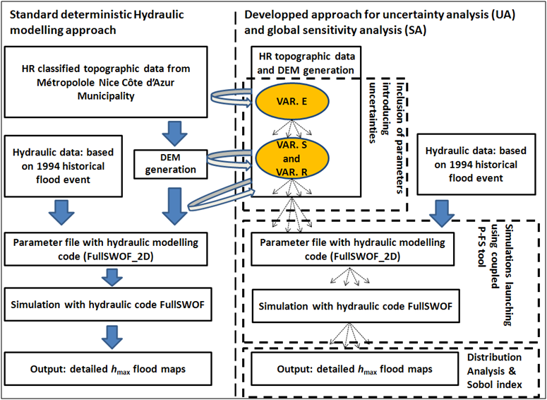
Figure 1: Implemented GSA approach.

Once simulations were completed with P-FS, GSA analysis has been carried out. First, the convergence of the results, in other word it has been checked that the number of simulations is large enough to generate a representative sample of the uncertainties associated to the studied source. Then uncertainties analysis was conducted, followed by the calculation of Sobol indices. The selected output of interest is the overland flow water surface elevation ($h_{max}+z$).

3 Results and discussion

3.1 Operational achievement of the approach

A performed version of P-FS couple allows to run simulations with selected set of input parameters (Var. $E$, $S$ and $R$). The coupled tool is operational on the Mésocentre HPC computation center and P-FS would be transposable over any common high performance computation cluster, requiring only slight changes in the coupling part of the codes. Through the use of R commands, it is possible to launch several calculations. Using “Daemons”, up to $30$ simulations can be launched at a time. The calculations running time of our simulation is significant. Indeed, this computation time is highly dependent of mesh resolution as the $dx$ will directly impact the CFL dependent $dt$. Over a $12$ cores node of the Mésocentre HPC, the computation time is $2$, $6$, $12$, $24$, $80$ hours respectively for $5$, $4$, $3$, $2$, $1\;\text{m}$ resolution grids. Using about $400,000$ CPU hours, it has been possible to run $1,500$ simulations. Out of these $1,500$ simulations, few runs (about $30$) have shown numerical errors leading to computational crash. These simulations have been removed from our set of simulations used to carry out the GSA. This will be clarified in future work, but errors are possibly due to numerical instabilities generated by important topographic gradient change at the boundary condition. This first data set of output allows us to carry out a first UA and GSA. The remaining $500$ simulations are mainly for $R1$ and $R2$ resolutions, which are the most resource-demanding simulations, and will be run in a close future using more than one HPC node per each run to decrease running time.

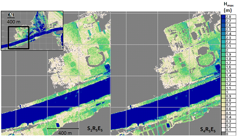
Figure 2: Illustration of $h_{max}$ value for two given simulations where Var. $S$ changes.

The variable of interest is the maximal water surface elevation ($h_{max}+z$) reached during a given simulation at different locations, with $h_{max}$ the maximal water depth reached at the point of interest and $z$ the DEM surface elevation at this point. The figure 2 illustrates the difference of $h_{max}+z$ obtained between two simulations when Var. $S$ varies. At different points of interest (see next section) difference in $h_{max}+z$ value can be significant. The analyses carried out over $40$ points of interests, highlight the influence of the selected variables. For example, for a given scenario when only Var. $E$ varies, an up to $0.5\;\text{m}$ difference in $h_{max}+z$ can be observed. Between all the $1,500$ scenarios a maximal difference of $1.26\;\text{m}$ in $h_{max}+z$ estimation at one of the point of interest is observed.

3.2 Local results for a point of interest

In the first place, a local analysis of the influence of topographic parameters has been achieved; $40$ points of interest have been selected and used for the analyses.

The convergence for Var. $E$ has been analyzed for the different points. As illustrated by figure 3(a), it appears that the distribution and the standard deviations of $h_{max}+z$, become stable with a sample size ($N$) of Var. $E$ is around $40$ to $50$. This gives qualitatively a first idea of what should be the minimum size of sample $N$ of Var. $E$ to allow performing reliable statistical analysis with an acceptable level of convergence.

To strengthen these findings, tests of convergence have been performed observing the evolution of mean $h_{max}+z$ value and the $95\%$ confidence interval (CI) when $N$ size increases. Figure 3(b) shows this result for a given point of interest. The analysis shows the sample size is above $30$, the mean and the CI become stable. It has to be noticed that similar results are obtained with the other selected points of interest, $30$ to $40$ realizations are sufficient to generate a representative sample of the uncertainties associated to the Var. $E$.

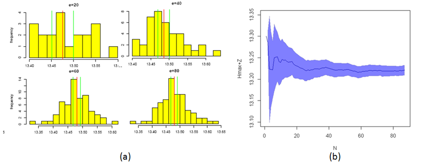
Figure 3: (a): Illustration of $h_{max}+z$ distribution and (b) convergence of mean and CI with fixed Var. $S$ and Var. $R$ when increasing sample of size of Var. $E$.

When looking at the output variable of interest $h_{max}+z$, it is relevant to check its distribution behavior for a fixed value of one of the two discrete input parameters (Var. $R$ or Var. $S$). This has been done with a subset of sample $N$ Var. $E$ equal to 50 for each discrete value of non fixed variables Var. $R$ and Var. $S$ (figure 4). This approach helps to make a qualitative description of the output distribution behavior relatively to the non fixed parameters. This test has been carried out for $40$ different points of interest. Figure 4 illustrates the main observations which can be effectuated using different distribution plots for fixed Var. $R$ or for fixed value of Var. $S$. Results show that for a given value of Var. $R$, Var. $E$ impact over variability of $h_{max}+z$ is relatively less significant than the impact of Var. $S$ (discrete choices). It has also been observed that increasing the level of geometric details included in DEM (Var. $S$) will not involve linear variations in $h_{max}+z$ values. Indeed, detailed above ground feature implementation lead to more local effects in terms of overland flow path modification and consequently, highly impact local $h_{max}+z$ values. When focusing on $h_{max}+z$ distribution for varying discrete mesh resolution (Var. $R$) for a given fixed Var. $S$ value (figure 4), it is observed that, comparatively to effect of Var. $E$ in output distribution, the influence generated by Var. $R$ on $h_{max}+z$ values is negligible. This finding does not consider the finest Var. $R$ ($1\;\text{m}$) as less than $50$ realizations of Var. $E$ were available so far with these resolutions.

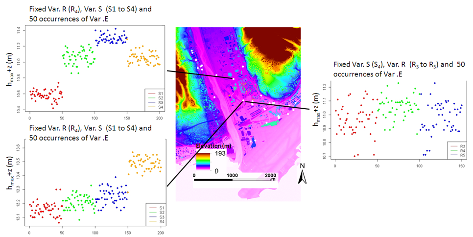
Figure 4: Output ($h_{max}+z$) distribution plots at two points of interest with one fixed value (either Var. $S$ or Var. $R$).

The final step of the GSA approach calculates the Sobol indices (Figure 5). As mentioned previously Var. $R1$ has not been considered for the calculation. The parameter which influences the most $h_{max}+z$ is Var. $S$. Concerning the Sobol indices, it has to be mentioned that the sum of Sobol indices should be one, in our case the sum is smaller than one. Similar results have been highlighted by [Iooss, 2011]. This finding is due to the parameters cross variation. Moreover the inclusion of results at the highest resolution ($1\;\text{m}$) might increase the cross variation effects. These promising results for analysis are already useful and further analysis to observe cross variation effects as well as spatial variation of Sobol index are in progress. So far it can be observed that $32$ of the $40$ points of interest have Var. $S$ with the highest Sobol index and $8$ points have Var. $R$ with the highest Sobol index. These two parameters are modeller choices. In the $32$ cases where Var. $S$ has the highest Sobol Index, $50\%$ of the points have Var. $R$ in the second rank and $50\%$ Var. $E$.

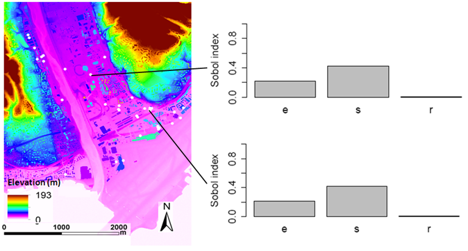
Figure 5: First-order Sobol indices for two selected points.

3.3 Perspectives and analyze for further work

One of the main advantages of two-dimensional hydraulic models is their spatial distribution over the area modeled. Therefore, uncertainties related to topography variability can be spatially represented for the Var river valley. Sobol index maps are presented in figure 6 over a sub-area. In a near future and integrate cross variation effect.

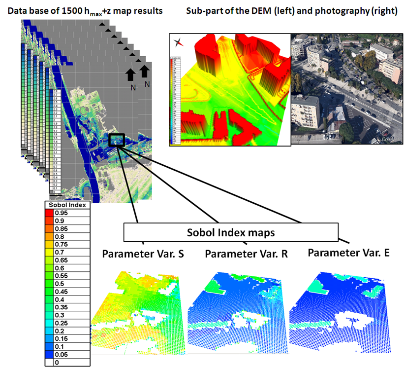
Figure 6: Sobol index maps over $150\;\text{m}$ long per $200\;\text{m}$ large part of the domain.

Nevertheless, as it has been mentioned, our representation of Var. $E$, using a spatially uniform distribution function of average measurement error is a first simple approximation. Indeed, the average error is a spatially varying function of physical properties (slope notably). Assigning differents spatially varying parameters of Var. $E$ distribution function would be a more sophisticated approach. Moreover, errors in photo-interpretation, which will spatially impact Var. $S$, deserve to be investigated as well.

4 Conclusions

In this study, a GSA is performed based on Sobol sensitivity analysis to quantify the uncertainties related to high resolution topography data inclusion in two-dimensional hydraulic model. Input parameters considered in the study encompass both measurement errors, and modeller choices for high resolution topographic data used in models. The applied GSA method relies ($i$) on the use of a specific tool coupling a parametric environment with a 2D hydraulic modelling tool Prométhée-FullSWOF_2D, and ($ii$) on the use of high performance computation resources. The implemented approach is able to highlight the uncertainties generated by topography parameters and operator choices when including high resolution data in hydraulic models.

$1,500$ simulations have been effectuated at this stage of the study. Convergence of the approach is checked and output distribution analyzed for qualitative apprehension of input parameters local effects on maximal computed overland flow ($h_{max}+z$). The major source of uncertainty related to water elevation $h_{max}+z$ is the modeller choice Var. $S$ which is the choice of operator regarding above ground features included in DEM used for hydraulic simulation. Errors related to measurement Var. $E$ significantly impact variability of $h_{max}+z$ model outputs but in a relatively smaller extent. Regarding Var. $R$, further investigations will be undertaken when more realizations will be available. Overall, these results confirm the relative importance of the uncertainty in topography input data. The main limits of the approach are concerning the way Var. $E$ and Var. $S$ are integrated in the analysis. Future work will be focused on the design of Sobol map index over the whole flood extent.

References

- [Abily et al., 2013a] Abily, M., Duluc, C. M., Faes, J. B., and Gourbesville, P. (2013a). Performance assessment of modelling tools for high resolution runoff simulation over an industrial site. Journal of Hydroinformatics, 15(4):1296–1311.
- [Abily et al., 2013b] Abily, M., Gourbesville, Andres, L., and Duluc, C.-M. (2013b). Photogrammetric and LiDAR data for high resolution runoff modeling over industrial and urban sites. In Zhaoyin, W., Lee, J. H.-w., Jizhang, G., and Shuyou, C., editors, Proceedings of the 35th IAHR World Congress, September 8-13, 2013, Chengdu, China. Tsinghua University Press, Beijing.
- [Andres, 2012] Andres, L. (2012). L’apport de la donnée topographique pour la modélisation 3d fine et classifiée d’un territoire. Revue XYZ, 133 - 4e trimestre:24–30.
- [ASN, 2013] ASN (2013). Protection of Basic Nuclear Installations Against External Flooding - guide no.13 - version of 08/01/2013. Technical report, Autorité de Sûreté Nucléaire.
- [Cordier, S. et al., 2013] Cordier, S., Coullon, H., Delestre, O., Laguerre, C., Le, M. H., Pierre, D., and Sadaka, G. (2013). FullSWOF Paral: Comparison of two parallelization strategies (MPI and SkelGIS) on a software designed for hydrology applications. ESAIM: Proc., 43:59–79.
- [Delestre et al., 2014a] Delestre, O., Cordier, S., Darboux, F., Du, M., James, F., Laguerre, C., Lucas, C., and Planchon, O. (2014a). FullSWOF: A software for overland flow simulation. In Gourbesville, P., Cunge, J., and Caignaert, G., editors, Advances in Hydroinformatics, Springer Hydrogeology, pages 221–231. Springer Singapore.
- [Delestre et al., 2014b] Delestre, O., Darboux, F., James, F., Lucas, C., Laguerre, C., and Cordier, S. (2014b). FullSWOF: A free software package for the simulation of shallow water flows. Research report, MAPMO, université d’Orléans ; Institut National de la Recherche Agronomique. 38 pages.
- [Egels and Kasser, 2004] Egels, Y. and Kasser, M. (2004). Digital Photogrammetry. Taylor & Francis.
- [Guinot and Gourbesville, 2003] Guinot, V. and Gourbesville, P. (2003). Calibration of physically based models: back to basics? Journal of Hydroinformatics, 5(4):233–244.
- [Herman et al., 2013] Herman, J., Kollat, J., Reed, P., and Wagener, T. (2013). Technical note: Method of Morris effective reduces the computational demands of global sensitivity analysis for distributed watershed models. Hydrology and Earth System Sciences, 17:2893–2903.
- [Ihaka, 1998] Ihaka, R. (1998). R: Past and future history. A Draft of a Paper for Interface ’98.
- [Iooss, 2011] Iooss, B. (2011). Revue sur l’analyse de sensibilité globale de modèles numériques. Journal de la Société Française de Statistique, 152(1):1–23.
- [Lafarge et al., 2010] Lafarge, F., Descombes, X., Zerubia, J., and Pierrot-Deseilligny, M. (2010). Structural approach for building reconstruction from a single DSM. Trans. on Pattern Analysis and Machine Intelligence, IEEE, 32(1):135–147.
- [Lafarge and Mallet, 2011] Lafarge, F. and Mallet, C. (2011). Building large urban environments from unstructured point data. In Computer Vision (ICCV), 2011 IEEE International Conference, volume 0, pages 1068–1075, Los Alamitos, CA, USA. IEEE Computer Society.
- [Lavabre et al., 1996] Lavabre, J., Mériaux, P., Nicoletis, E., and Cardelli, B. (1996). La crue catastrophique du Var du 5 novembre 1994/ Catastrophic Var river flood of 5 november 1994. In Convegno internazionale la prevenzione delle catastrofi idrogeologichi il contributo della ricerca scientifica, Alba, ITA, 5-7 nivembre 1996. 5 pages.
- [Lu and Weng, 2007] Lu, D. and Weng, Q. (2007). A survey of image classification methods and techniques for improving classification performance. International Journal of Remote Sensing, 28(5):823–870.
- [Mastin et al., 2009] Mastin, A., Kepner, J., and Fisher, J. I. (2009). Automatic Registration of LIDAR and Optical Images of Urban Scenes. In Computer Vision and Pattern Recognition, 2009. CVPR 2009. IEEE Conference on, pages 2639–2646.
- [Musialski et al., 2013] Musialski, P., Wonka, P., Aliaga, D. G., Wimmer, M., van Gool, L., and Purgathofer, W. (2013). A survey of urban reconstruction. Computer Graphics Forum, 32(6):146–177.
- [Nex and Remondino, 2013] Nex, F. and Remondino, F. (2013). UAV for 3D mapping applications: a review. Applied Geomatics, pages 1–15.
- [Nguyen et al., 2015] Nguyen, T.-m., Richet, Y., Balayn, P., and Bardet, L. (2015). Propagation des incertitudes dans les modèles hydrauliques 1D. La Houille Blanche, 5:55–62.
- [Remondino et al., 2011] Remondino, F., Barazzetti, L., Nex, F., Scaioni, M., and Sarazzi, D. (2011). UAV photogrammetry for mapping and 3D modeling – Current status and future perspectives. In Archives of Photogrammetry, Remote Sensing and Spatial Information Sciences, volume 38(1/C22). ISPRS Conference UAV-g, Zurich, Switzerland.
- [Saint-Geours, 2012] Saint-Geours, N. (2012). Analyse de sensibilité de modèles spatialisés - Application à l’analyse coût-bénéfice de projets de prévention des inondations. Thèse, Université Montpellier II - Sciences et Techniques du Languedoc.
- [Tsubaki and Fujita, 2010] Tsubaki, R. and Fujita, I. (2010). Unstructured grid generation using LiDAR data for urban flood inundation modelling. Hydrological Processes, 24:1404–1420.