BlockQuicksort: How Branch Mispredictions don’t affect Quicksort

Abstract.

Since the work of Kaligosi and Sanders (2006), it is well-known that Quicksort – which is commonly considered as one of the fastest in-place sorting algorithms – suffers in an essential way from branch mispredictions. We present a novel approach to address this problem by partially decoupling control from data flow: in order to perform the partitioning, we split the input in blocks of constant size (we propose 128 data elements); then, all elements in one block are compared with the pivot and the outcomes of the comparisons are stored in a buffer. In a second pass, the respective elements are rearranged. By doing so, we avoid conditional branches based on outcomes of comparisons at all (except for the final Insertionsort). Moreover, we prove that for a static branch predictor the average total number of branch mispredictions is at most $\epsilon n\log n+\mathcal{O}(n)$ for some small $\epsilon$ depending on the block size when sorting $n$ elements.

Our experimental results are promising: when sorting random integer data, we achieve an increase in speed (number of elements sorted per second) of more than 80% over the GCC implementation of C++ std::sort. Also for many other types of data and non-random inputs, there is still a significant speedup over std::sort. Only in few special cases like sorted or almost sorted inputs, std::sort can beat our implementation. Moreover, even on random input permutations, our implementation is even slightly faster than an implementation of the highly tuned Super Scalar Sample Sort, which uses a linear amount of additional space.

1. Introduction

Sorting a sequence of elements of some totally ordered universe remains one of the most fascinating and well-studied topics in computer science. Moreover, it is an essential part of many practical applications. Thus, efficient sorting algorithms directly transfer to a performance gain for many applications. One of the most widely used sorting algorithms is Quicksort, which has been introduced by Hoare in 1962 [14] and is considered to be one of the most efficient sorting algorithms. For sorting an array, it works as follows: first, it chooses an arbitrary pivot element and then rearranges the array such that all elements smaller than the pivot are moved to the left side and all elements larger than the pivot are moved to the right side of the array – this is called partitioning. Then, the left and right side are both sorted recursively. Although its average number of comparisons is not optimal – $1{.}38n\log n+\mathcal{O}(n)$ vs. $n\log n+\mathcal{O}(n)$ for Mergesort –, its over-all instruction count is very low. Moreover, by choosing the pivot element as median of some larger sample, the leading term $1{.}38n\log n$ for the average number of comparisons can be made smaller – even down to $n\log n$ when choosing the pivot as median of some sample of growing size [21]. Other advantages of Quicksort are that it is easy to implement and that it does not need extra memory except the recursion stack of logarithmic size (even in the worst case if properly implemented). A major drawback of Quicksort is its quadratic worst-case running time. Nevertheless, there are efficient ways to circumvent a really bad worst-case. The most prominent is Introsort (introduced by Musser [22]) which is applied in GCC implementation of std::sort: as soon as the recursion depth exceeds a certain limit, the algorithm switches to Heapsort.

Another deficiency of Quicksort is that it suffers from branch mispredictions (or branch misses) in an essential way. On modern processors with long pipelines (14 stages for Intel Haswell, Broadwell, Skylake processors – for the older Pentium 4 processors even more than twice as many) every branch misprediction causes a rather long interruption of the execution since the pipeline has to be filled anew. In [15], Kaligosi and Sanders analyzed the number of branch mispredictions incurred by Quicksort. They examined different simple branch prediction schemes (static prediction and 1-bit, 2-bit predictors) and showed that with all of them, Quicksort with a random element as pivot causes on average $cn\log n+\mathcal{O}(n)$ branch mispredictions for some constant $c=0{.}34$ (resp. $c=0{.}46$, $c=0{.}43$). In particular, in Quicksort with random pivot element, every fourth comparison is followed by a mispredicted branch. The reason is that for partitioning, each element is compared with the pivot and depending on the outcome either it is swapped with some other element or not. Since for an optimal pivot (the median), the probability of being smaller the pivot is $50\%$, there is no way to predict these branches.

Kaligosi and Sanders also established that choosing skewed pivot elements (far off the median) might even decrease the running time because it makes branches more predictable. This also explains why, although theoretically larger samples for pivot selection were shown to be superior, in practice the median-of three variant turned out to be the best. In [6], the skewed pivot phenomenon is confirmed experimentally. Moreover, in [20], precise theoretical bounds on the number of branch misses for Quicksort are given – establishing also theoretical superiority of skewed pivots under the assumption that branch mispredictions are expensive.

In [8] Brodal and Moruz proved a general lower bound on the number of branch mispredictions given that every comparison is followed by a conditional branch which depends on the outcome of the comparison. In this case there are $\Omega(n\log_{d}n)$ branch mispredictions for a sorting algorithm which performs $\mathcal{O}(dn\log n)$ comparisons. As Elmasry and Katajainen remarked in [10], this theorem does not hold anymore if the results of comparisons are not used for conditional branches. Indeed, they showed that every program can be transformed into a program which induces only a constant number of branch misses and whose running time is linear in the running time of the original program. However, this general transformation introduces a huge constant factor overhead. Still, in [10] and [11] Elmasry, Katajainen and Stenmark showed how to efficiently implement many algorithms related to sorting with only few branch mispredictions. They call such programs lean. In particular, they present variants of Mergesort and Quicksort suffering only very little from branch misses. Their Quicksort variant (called Tuned Quicksort, for details on the implementation, see [16]) is very fast for random permutations – however, it does not behave well with duplicate elements because it applies Lomuto’s uni-directional partitioner (see e. g. [9]).

Another development in recent years is multi-pivot Quicksort (i. e. several pivots in each partitioning stage [4, 5, 18, 27, 28]). It started with the introduction of Yaroslavskiy’s dual-pivot Quicksort [30] – which, surprisingly, was faster than known Quicksort variants and, thus, became the standard sorting implementation in Oracle Java 7 and Java 8. Concerning branch mispredictions all these multi-pivot variants behave essentially like ordinary Quicksort [20]; however, they have one advantage: every data element is accessed only a few times (this is also referred to as the number of scans). As outlined in [5], increasing the number of pivot elements further (up to 127 or 255), leads to Super Scalar Sample Sort, which has been introduced by Sanders and Winkel [24]. Super Scalar Sample Sort not only has the advantage of few scans, but also is based on the idea of avoiding conditional branches. Indeed, the correct bucket (the position between two pivot elements) can be found by converting the results of comparisons to integers and then simply performing integer arithmetic. In their experiments Sanders and Winkel show that Super Scalar Sample Sort is approximately twice as fast as Quicksort (std::sort) when sorting random integer data. However, Super Scalar Sample Sort has one major draw-back: it uses a linear amount of extra space (for sorting $n$ data elements, it requires space for another $n$ data elements and additionally for more than $n$ integers). In the conclusion of [15], Kaligosi and Sander raised the question:

However, an in-place sorting algorithm that is better than Quicksort with skewed pivots is an open problem.

(Here, in-place means that it needs only a constant or logarithmic amount of extra space.) In this work, we solve the problem by presenting our block partition algorithm, which allows to implement Quicksort without any branch mispredictions incurred by conditional branches based on results of comparisons (except for the final Insertionsort – also there are still conditional branches based on the control-flow, but their amount is relatively small). We call the resulting algorithm BlockQuicksort. Our work is inspired by Tuned Quicksort from [11], from where we also borrow parts of our implementation. The difference is that by doing the partitioning block-wise, we can use Hoare’s partitioner, which is far better with duplicate elements than Lomuto’s partitioner (although Tuned Quicksort can be made working with duplicates by applying a check for duplicates similar to what we propose for BlockQuicksort as one of the further improvements in Section 3.2). Moreover, BlockQuicksort is also superior to Tuned Quicksort for random permutations of integers.

Our Contributions

• We present a variant of the partition procedure that only incurs few branch mispredictions by storing results of comparisons in constant size buffers.

• We prove an upper bound of $\epsilon n\log n+\mathcal{O}(n)$ branch mispredictions on average, where $\epsilon<\frac{1}{16}$ for our proposed block size (Theorem 3.1).

• We propose some improvements over the basic version.

• We implemented our algorithm with an stl-style interface.

• We conduct experiments and compare BlockQuicksort with std::sort, Yaroslavskiy’s dual-pivot Quicksort and Super Scalar Sample Sort – on random integer data it is faster than all of these and also Katajainen et al.’s Tuned Quicksort.

Outline

Section 2 introduces some general facts on branch predictors and mispredictions, and gives a short account of standard improvements of Quicksort. In Section 3, we give a precise description of our block partition method and establish our main theoretical result – the bound on the number of branch mispredictions. Finally, in Section 4, we experimentally evaluate different block sizes, different pivot selection strategies and compare our implementation with other state of the art implementations of Quicksort and Super Scalar Sample Sort.

2. Preliminaries

Logarithms denoted by $\log$ are always base 2. The term average case refers to a uniform distribution of all input permutations assuming all elements are different. In the following std::sort always refers to its GCC implementation.

Branch Misses

Branch mispredictions can occur when the code contains conditional jumps (i. e. if statements, loops, etc.). Whenever the execution flow reaches such a statement, the processor has to decide in advance which branch to follow and decode the subsequent instructions of that branch. Because of the length of the pipeline of modern microprocessors, a wrong predicted branch causes a large delay since, before continuing the execution, the instructions for the other branch have to be decoded.

Branch Prediction Schemes

Precise branch prediction schemes of most modern processors are not disclosed to the public. However, the simplest schemes suffice to make BlockQuicksort induce only few mispredictions.

The easiest branch prediction scheme is the static predictor: for every conditional jump the compiler marks the more likely branch. In particular, that means that for every if statement, we can assume that there is a misprediction if and only if the if branch is not taken; for every loop statement, there is precisely one misprediction for every time the execution flow reaches that loop: when the execution leaves the loop. For more information about branch prediction schemes, we refer to [13, Section 3.3].

How to avoid Conditional Branches

The usual implementation of sorting algorithms performs conditional jumps based on the outcome of comparisons of data elements. There are at least two methods how these conditional jumps can be avoided – both are supported by the hardware of modern processors:

• Conditional moves (CMOVcc instructions on x86 processors) – or, more general, conditional execution. In C++ compilation to a conditional move can be (often) triggered by

  ⬇

  i = (x < y) ? j : i;

• Cast Boolean variables to integer (SETcc instructions x86 processors). In C++:

  ⬇

  int i = (x < y);

Also many other instruction sets support these methods (e. g. ARM [1], MIPS [23]). Still, the Intel Architecture Optimization Reference Manual [2] advises only to use these instructions to avoid unpredictable branches (as it is the case for sorting) since correctly predicted branches are still faster. For more examples how to apply these methods to sorting, see [11].

Quicksort and improvements

The central part of Quicksort is the partitioning procedure. Given some pivot element, it returns a pointer $p$ to an element in the array and rearranges the array such that all elements left of the $p$ are smaller or equal the pivot and all elements on the right are greater or equal the pivot. Quicksort first chooses some pivot element, then performs the partitioning, and, finally, recurses on the elements smaller and larger the pivot – see Algorithm 1. We call the procedure which organizes the calls to the partitioner the Quicksort main loop.

Algorithm 1 Quicksort

1:procedure Quicksort($A[\ell,\dots,r]$)

2:    if $r>\ell$ then

3:         pivot $\leftarrow$ choosePivot($A[\ell,\dots,r]$)

4:         cut $\leftarrow$ partition($A[\ell,\dots,r]$, pivot)

5:         Quicksort($A[\ell,\dots,\mathrm{cut}-1]$)

6:         Quicksort($A[\mathrm{cut},\dots,r]$)

7:    end if

8:end procedure

There are many standard improvements for Quicksort. For our optimized Quicksort main loop (which is a modified version of Tuned Quicksort [11, 16]), we implemented the following:

• A very basic optimization due to Sedgewick [26] avoids recursion partially (e. g. std::sort) or totally (here – this requires the introduction of an explicit stack).

• Introsort [22]: there is an additional counter for the number of recursion levels. As soon as it exceeds some bound (std::sort uses $2\log n$ – we use $2\log n+3$), the algorithms stops Quicksort and switches to Heapsort [12, 29] (only for the respective sub-array). By doing so, a worst-case running time of $\mathcal{O}(n\log n)$ is guaranteed.

• Sedgewick [26] also proposed to switch to Insertionsort (see e. g. [17, Section 5.2.1]) as soon as the array size is less than some fixed small constant (16 for std::sort and our implementation). There are two possibilities when to apply Insertionsort: either during the recursion, when the array size becomes too small, or at the very end after Quicksort has finished. We implemented the first possibility (in contrast to std::sort) because for sorting integers, it hardly made a difference, but for larger data elements there was a slight speedup (in [19] this was proposed as memory-tuned Quicksort).

• After partitioning, the pivot is moved to its correct position and not included in the recursive calls (not applied in std::sort).

• The basic version of Quicksort uses a random or fixed element as pivot. A slight improvement is to choose the pivot as median of three elements – typically the first, in the middle and the last. This is applied in std::sort and many other Quicksort implementations. Sedgewick [26] already remarked that choosing the pivots from an even larger sample does not provide a significant increase of speed. In view of the experiments with skewed pivots [15], this is no surprise. For BlockQuicksort, a pivot closer to the median turns out to be beneficial (Figure 2 in Section 4). Thus, it makes sense to invest more time to find a better pivot element. In [21], Martinez and Roura show that the number of comparisons incurred by Quicksort is minimal if the pivot element is selected as median of $\Theta(\sqrt{n})$ elements. Another variant is to choose the pivot as median of three (resp. five) elements which themselves are medians of of three (resp. five) elements. We implemented all these variants for our experiments – see Section 4.

Our main contribution is the block partitioner, which we describe in the next section.

3. Block Partitioning

The idea of block partitioning is quite simple. Recall how Hoare’s original partition procedure works (Algorithm 2):

Algorithm 2 Hoare’s Partitioning

1:procedure Partition($A[\ell,\dots,r]$, pivot)

2:    while $\ell<r$ do

3:         while $A[\ell]<\mathrm{pivot}$ do $\ell{+}\!\!\;{+}$ end while

4:         while $A[r]>\mathrm{pivot}$ do $r{-}\!\!\;{-}$ end while

5:         if $\ell<r$ then  swap($A[\ell],A[r]$); $\ell{+}\!\!\;{+}$; $r{-}\!\!\;{-}$ end if

6:    end while

7:    return $\ell$

8:end procedure

Two pointers start at the leftmost and rightmost elements of the array and move towards the middle. In every step the current element is compared to the pivot (Line 3 and 4). If some element on the right side is less or equal the pivot (resp. some element on the left side is greater or equal), the respective pointer stops and the two elements found this way are swapped (Line 5). Then the pointers continue moving towards the middle.

The idea of BlockQuicksort (Algorithm 3) is to separate Lines 3 and 4 of Algorithm 2 from Line 5: fix some block size $B$; we introduce two buffers $\mathrm{offsets}_{L}[0,\dots,B-1]$ and $\mathrm{offsets}_{R}[0,\dots,B-1]$ for storing pointers to elements ($\mathrm{offsets}_{L}$ will store pointers to elements on the left side of the array which are greater or equal than the pivot element – likewise $\mathrm{offsets}_{R}$ for the right side). The main loop of Algorithm 3 consists of two stages: the scanning phase (Lines 5 to 18) and the rearrangement phase (Lines 19 to 26).

Algorithm 3 Block partitioning

1:procedure BlockPartition($A[\ell,\dots,r]$, pivot)

2:    integer $\mathrm{offsets}_{L}[0,\dots,B-1],\mathrm{offsets}_{R}[0,\dots,B-1]$

3:    integer $\mathrm{start}_{L},\mathrm{start}_{R},\mathrm{num}_{L},\mathrm{num}_{R}\leftarrow 0$

4:    while $r-\ell+1>2B$ do$\triangleright$ start main loop

5:         if $\mathrm{num}_{L}=0$ then$\triangleright$ if left buffer is empty, refill it

6:             $\mathrm{start}_{L}\leftarrow 0$

7:             for $i=0,\dots,B-1$ do

8:                 $\mathrm{offsets}_{L}[\mathrm{num}_{L}]\leftarrow i$

9:                 $\mathrm{num}_{L}\mathrel{{+}\!\!\;{=}}(\mathrm{pivot}\geq A[\ell+i])$$\triangleright$ scanning phase for left side

10:             end for

11:         end if

12:         if $\mathrm{num}_{R}=0$ then$\triangleright$ if right buffer is empty, refill it

13:             $\mathrm{start}_{R}\leftarrow 0$

14:             for $i=0,\dots,B-1$ do

15:                 $\mathrm{offsets}_{R}[\mathrm{num}_{R}]\leftarrow i$

16:                 $\mathrm{num}_{R}\mathrel{{+}\!\!\;{=}}(\mathrm{pivot}\leq A[r-i])$ $\triangleright$ scanning phase for right side

17:             end for

18:         end if

19:         integer num $=\min(\mathrm{num}_{L},\mathrm{num}_{R})$

20:         for $j=0,\dots,\mathrm{num}-1$ do

21:             swap($A\bigl{[}\ell+\mathrm{offsets}_{L}[\mathrm{start}_{L}+j]\bigr{]},A\bigl{[}r-\mathrm{offsets}_{R}[\mathrm{start}_{R}+j]\bigr{]}$)$\triangleright$ rearrangement phase

22:         end for

23:         $\mathrm{num}_{L},\mathrm{num}_{R}\mathrel{{-}\!\!\;{=}}\mathrm{num}$; $\mathrm{start}_{L},\mathrm{start}_{R}\mathrel{{+}\!\!\;{=}}\mathrm{num}$

24:         if $(\mathrm{num}_{L}=0)$ then $\ell\mathrel{{+}\!\!\;{=}}B$ end if

25:         if $(\mathrm{num}_{R}=0)$ then $r\mathrel{{-}\!\!\;{=}}B$ end if

26:    end while$\triangleright$ end main loop

27:    compare and rearrange remaining elements

28:end procedure

Like for classical Hoare partition, we also start with two pointers (or indices as in the pseudocode) to the leftmost and rightmost element of the array. First, the scanning phase takes place: the buffers which are empty are refilled. In order to do so, we move the respective pointer towards the middle and compare each element with the pivot. However, instead of stopping at the first element which should be swapped, only a pointer to the element is stored in the respective buffer (Lines 8 and 9 resp. 15 and 16 – actually the pointer is always stored, but depending on the outcome of the comparison a counter holding the number of pointers in the buffer is increased or not) and the pointer continues moving towards the middle. After an entire block of $B$ elements has been scanned (either on both sides of the array or only on one side), the rearranging phase begins: it starts with the first positions of the two buffers and swaps the data elements they point to (Line 21); then it continues until one of the buffers contains no more pointers to elements which should be swapped. Now the scanning phase is restarted and the buffer that has run empty is filled again.

The algorithm continues this way until fewer elements than two times the block size remain. Now, the simplest variant is to switch to the usual Hoare partition method for the remaining elements (in the experiments with suffix Hoare finish). But, we also can continue with the idea of block partitioning: the algorithm scans the remaining elements as one or two final blocks (of smaller size) and performs a last rearrangement phase. After that, some elements to swap in one of the two buffers might still remain, while the other buffer is empty. With one run through the buffer, all these elements can be moved to the left resp. right (similar as it is done in the Lomuto partitioning method, but without performing actual comparisons). We do not present the details for this final rearranging here because on one hand it gets a little tedious and on the other hand it does neither provide a lot of insight into the algorithm nor is it necessary to prove our result on branch mispredictions. The C++ code of this basic variant can be found in Appendix B.

3.1. Analysis

If the input consists of random permutations (all data elements different), the average numbers of comparisons and swaps are the same as for usual Quicksort with median-of-three. This is because both Hoare’s partitioner and the block partitioner preserve randomness of the array.

The number of scanned elements (total number of elements loaded to the registers) is increased by two times the number of swaps, because for every swap, the data elements have to be loaded again. However, the idea is that due to the small block size, the data elements still remain in L1 cache when being swapped – so the additional scan has no negative effect on the running time. In Section 4 we see that for larger data types and from a certain threshold on, an increasing size of the blocks has a negative effect on the running time. Therefore, the block size should not be chosen too large – we propose $B=128$ and fix this constant throughout (thus, already for inputs of moderate size, the buffers also do not require much more space than the stack for Quicksort).

Branch mispredictions

The next theorem is our main theoretical result. For simplicity we assume here that BlockQuicksort is implemented without the worst-case-stopper Heapsort (i. e. there is no limit on the recursion depth). Since there is only a low probability that a high recursion depth is reached while the array is still large, this assumption is not a real restriction. We analyze a static branch predictor: there is a misprediction every time a loop is left and a misprediction every time the if branch of an if statement is not taken.

Theorem 3.1.

Let $\mathcal{C}$ be the average number of comparisons of Quicksort with constant size pivot sample. Then BlockQuicksort (without limit to the recursion depth and with the same pivot selection method) with blocksize $B$ induces at most $\frac{6}{B}\cdot\mathcal{C}+\mathcal{O}(n)$ branch mispredictions on average. In particular, BlockQuicksort with median-of-three induces less then $\frac{8}{B}n\log n+\mathcal{O}(n)$ branch mispredictions on average.

Theorem 3.1 shows that when choosing the block size sufficiently large, the $n\log n$-term becomes very small and – for real-world inputs – we can basically assume a linear number of branch mispredictions. Moreover, Theorem 3.1 can be generalized to samples of non-constant size for pivot selection. Since the proof might become tedious, we stick to the basic variant here. The constant 6 in Theorem 3.1 can be replaced by 4 when implementing Lines 19, 24, and 25 of Algorithm 3 with conditional moves.

Proof 3.2.

First, we show that every execution of the block partitioner Algorithm 3 on an array of length $n$ induces at most $\frac{6}{B}n+c$ branch mispredictions for some constant $c$. In order to do so, we only need to look at the main loop (Line 4 to 27) of Algorithm 3 because the final scanning and rearrangement phases consider only a constant (at most $2B$) number of elements. Inside the main loop there are three for loops (starting Lines 7, 14, 20), four if statements (starting Lines 5, 12, 24, 25) and the min calculation (whose straightforward implementation is an if statement – Line 19). We know that in every execution of the main loop at least one of the conditions of the if statements in Line 5 and 12 is true because in every rearrangement phase at least one buffer runs empty. The same holds for the two if statements in Line 24 and 25. Therefore, we obtain at most two branch mispredictions for the ifs, three for the for loops and one for the min in every execution of the main loop.

In every execution of the main loop, there are at least $B$ comparisons of elements with the pivot. Thus, the number of branch misses in the main loop is at most $\frac{6}{B}$ times the number of comparisons. Hence, for every input permutation the total number of branch mispredictions of BlockQuicksort is at most $\frac{6}{B}\cdot\#\mathrm{comparisons}+(c+c^{\prime})\cdot\#\mathrm{calls\ to\ partition}+\mathcal{O}(n),$ where $c^{\prime}$ it the number of branch mispredictions of one execution of the main loop of Quicksort (including pivot selection, which only needs a constant number of instructions) and the $\mathcal{O}(n)$ term comes from the final Insertionsort. The number of calls to partition is bounded by $n$ because each element can be chosen as pivot only once (since the pivots are not contained in the arrays for the recursive calls). Thus, by taking the average over all input permutations, the first statement follows.

The second statement follows because Quicksort with median-of-three incurs $1{.}18n\log n+\mathcal{O}(n)$ comparisons on average [25].

Remark 3.3.

The $\mathcal{O}(n)$-term in Theorem 3.1 can be bounded by $3n$ by taking a closer look to the final rearranging phase.

We give a rough heuristic estimate: it is save to assume that the average length of arrays on which Insertionsort is called is at least 8 (recall that we switch to Insertionsort as soon as the array size is less than 17). For Insertionsort there is one branch miss for each element (when exiting the loop for finding the position) plus one for each call of Insertionsort (when exiting the loop over all elements to insert). Furthermore, there are at most two branch misses in the main Quicksort loop (Lines 177 and 196 in Appendix B) for every call to Insertionsort. Hence, we have approximately $\frac{11}{8}n$ branch misses due to Insertionsort.

It remains to count the constant number of branch misprediction incurred during every call of partitioning: After exiting the main loop of block partition, there is one more scan and rearrangement phase with a smaller block size. This leads to at most $\leq 7$ branch mispredictions (one extra because there is an additional case that both buffers are empty). The final rearranging incurs at most three branch misses (Lines 118, 136, 140). Selecting the pivot as median-of-three (Line 11) induces no branch misses since all conditional statements are compiled to conditional moves. Finally, there is at most one branch miss in the main Quicksort loop for every call to partition (Line 180). This sums up to at most $13$ branch misses per call to partition. Because the average size of arrays treated by Insertionsort is at least 8, the number of calls to partition is less than $n/8$.

Thus, in total the $\mathcal{O}(n)$-term in Theorem 3.1 consists of at most $\frac{11}{8}n+\frac{13}{8}n=3n$ branch mispredictions.

3.2. Further Tuning of Block Partitioning

We propose and implemented further tunings for our block partitioner:

1. Loop unrolling: since the block size is a power of two, the loops of the scanning phase can be unrolled four or even eight times without causing additional overhead.

2. Cyclic permutations instead of swaps: We replace

   1:for $j=0,\dots,\mathrm{num}-1$ do

   2:    swap($A\bigl{[}\ell+\mathrm{offsets}_{L}[\mathrm{start}_{L}+j]\bigr{]},A\bigl{[}r-\mathrm{offsets}_{R}[\mathrm{start}_{R}+j]\bigr{]}$)

   3:end for

   by the following code, which does not perform exactly the same data movements, but still in the end all elements less than the pivot are on the left and all elements greater are on the right:

   1:temp $\leftarrow A\bigl{[}\ell+\mathrm{offsets}_{L}[\mathrm{start}_{L}]\bigr{]}$

   2:$A\bigl{[}\ell+\mathrm{offsets}_{L}[\mathrm{start}_{L}]\bigr{]}\leftarrow A\bigl{[}r-\mathrm{offsets}_{R}[\mathrm{start}_{R}]\bigr{]}$

   3:for $j=1,\dots,\mathrm{num}-1$ do

   4:    $A\bigl{[}r-\mathrm{offsets}_{R}[\mathrm{start}_{R}+j-1]\bigr{]}\leftarrow A\bigl{[}\ell+\mathrm{offsets}_{L}[\mathrm{start}_{L}+j]\bigr{]}$

   5:    $A\bigl{[}\ell+\mathrm{offsets}_{L}[\mathrm{start}_{L}+j]\bigr{]}\leftarrow A\bigl{[}r-\mathrm{offsets}_{R}[\mathrm{start}_{R}+j]\bigr{]}$

   6:end for

   7:$A\bigl{[}r-\mathrm{offsets}_{R}[\mathrm{start}_{R}+\mathrm{num}-1]\bigr{]}\leftarrow$ temp

   Note that this is also a standard improvement for partitioning – see e. g. [3].

In the following, we always assume these two improvements since they are of very basic nature (plus one more small change in the final rearrangement phase). We call the variant without them block_partition_simple – its C++ code can be found in Appendix B.

The next improvement is a slight change of the algorithm: in our experiments we noticed that for small arrays with many duplicates the recursion depth becomes often higher than the threshold for switching to Heapsort – a way to circumvent this is an additional check for duplicates equal to the pivot if one of the following two conditions applies:

• the pivot occurs twice in the sample for pivot selection (in the case of median-of-three),

• the partitioning results very unbalanced for an array of small size.

The check for duplicates takes place after the partitioning is completed. Only the larger half of the array is searched for elements equal to the pivot. This check works similar to Lomuto’s partitioner (indeed, we used the implementation from [16]): starting from the position of the pivot, the respective half of the array is scanned for elements equal to the pivot (this can be done by one less than comparison since elements are already known to be greater or equal (resp. less or equal) the pivot)). Elements which are equal to the pivot are moved to the side of the pivot. The scan continues as long as at least every fourth element is equal to the pivot (instead every fourth one could take any other ratio – this guarantees that the check stops soon if there are only few duplicates).

After this check, all elements which are identified as being equal to the pivot remain in the middle of the array (between the elements larger and the elements smaller than the pivot); thus, they can be excluded from further recursive calls. We denote this version with the suffix duplicate check (dc).

4. Experiments

We ran thorough experiments with implementations in C++ on different machines with different types of data and different kinds of input sequences. If not specified explicitly, the experiments are run on an Intel Core i5-2500K CPU (3.30GHz, 4 cores, 32KB L1 instruction and data cache, 256KB L2 cache per core and 6MB L3 shared cache) with 16GB RAM and operating system Ubuntu Linux 64bit version 14.04.4. We used GNU’s g++ (4.8.4); optimized with flags -O3 -march=native.

For time measurements, we used std::chrono::high_resolution_clock, for generating random inputs, the Mersenne Twister pseudo-random generator std::mt19937. All time measurements were repeated with the same 20 deterministically chosen seeds – the displayed numbers are the average of these 20 runs. Moreover, for each time measurement, at least 128MB of data were sorted – if the array size is smaller, then for this time measurement several arrays have been sorted and the total elapsed time measured. Our running time plots all display the actual time divided by the number of elements to sort on the y-axis.

We performed our running time experiments with three different data types:

• int: signed 32-bit integers.

• Vector: 10-dimensional array of 64-bit floating-point numbers (double). The order is defined via the Euclidean norm – for every comparison the sums of the squares of the components are computed and then compared.

• Record: 21-dimensional array of 32-bit integers. Only the first component is compared.

The code of our implementation of BlockQuicksort as well as the other algorithms and our running time experiments is available at https://github.com/weissan/BlockQuicksort.

Different Block Sizes

Figure 1 shows experimental results on random permutations for different data types and block sizes ranging from 4 up to $2^{24}$.

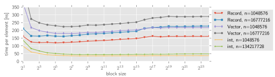
Figure 1. Different block sizes for random permutations.

We see that for integers only at the end there is a slight negative effect when increasing the block size. Presumably this is because up to a block size of $2^{19}$, still two blocks fit entirely into the L3 cache of the CPU. On the other hand for Vector a block size of 64 and for Record of 8 seem to be optimal – with a considerably increasing running time for larger block sizes.

As a compromise we chose to fix the block size to 128 elements for all further experiments. An alternative approach would be to choose a fixed number of bytes for one block and adapt the block size according to the size of the data elements.

Skewed Pivot Experiments

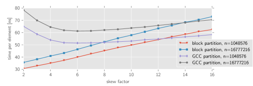
Figure 2. Sorting random permutations of 32-bit integers with skewed pivot. A skew factor $k$ means that $\left\lfloor\mathinner{\frac{n}{k}}\right\rfloor$-th element is chosen as pivot of an array of length $n$.

We repeated the experiments from [15] with skewed pivot for both the usual Hoare partitioner (std::__unguarded_partition, from the GCC implementation of std::sort) and our block partition method. For both partitioners we used our tuned Quicksort loop. The results can be seen in Figure 2: classic Quicksort benefits from skewed pivot, whereas BlockQuicksort works best with the exact median. Therefore, for BlockQuicksort it makes sense to invest more effort to find a good pivot.

Different Pivot Selection Methods

We implemented several strategies for pivot selection:

• median-of-three, median-of-five, median-of-twenty-three,

• median-of-three-medians-of-three, median-of-three-medians-of-five, median-of-five-medians-of-five: first calculate three (resp. five) times the median of three (resp. five) elements, then take the pivot as median of these three (resp. five) medians,

• median-of-$\sqrt{n}$.

All pivot selection strategies switch to median-of-three for small arrays. Moreover, the median-of-$\sqrt{n}$ variant switches to median-of-five-medians-of-five for arrays of length below 20000 (for smaller $n$ even the number of comparisons was better with median-of-five-medians-of-five). The medians of larger samples are computed with std::nth_element. Despite the results on skewed pivots Figure 2, there was no big difference between the different pivot selection strategies as it can be seen in Figure 3.

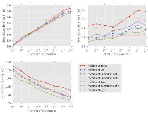
Figure 3. Different pivot selection strategies with random permutation. Upper left: Record; upper right: Vector; lower left: int. Be aware that the y-axis here displays the time divided by $n\log n$.

As expected, median-of-three was always the slowest for larger arrays. Median-of-five-medians-of-five was the fastest for int and median-of-$\sqrt{n}$ for Vector. We think that the small difference between all strategies is due to the large overhead for the calculation of the median of a large sample – and maybe because the array is rearranged in a way that is not favorable for the next recursive calls.

4.1. Comparison with other Sorting Algorithms

We compare variants of BlockQuicksort with the GCC implementation of std::sort (which is known to be one of the most efficient Quicksort implementations – see e. g. [7]), Yaroslavskiy’s dual-pivot Quicksort [30] (we converted the Java code of [30] to C++) and an implementation of Super Scalar Sample Sort [24] by Hübschle-Schneider. For random permutations and random values modulo $\sqrt{n}$, we also test Tuned Quicksort [16] and three-pivot Quicksort implemented by Aumüller and Bingmann from [5] (which is based on [18]) – for other types of inputs we omit these algorithms because of their poor behavior with duplicate elements.

Branch mispredictions

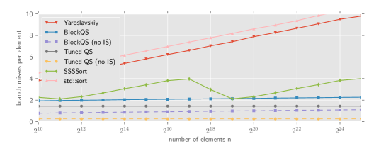
Figure 4. Number of branch mispredictions.

We experimentally determined the number of branch mispredictions of BlockQuicksort and the other algorithms with the chachegrind branch prediction profiler, which is part of the profiling tool valgrind. The results of these experiments on random int data can be seen in Figure 4 – the y-axis shows the number of branch misprediction divided the the array size. We only display the median-of-three variant of BlockQuicksort since all the variants are very much alike. We also added plots of BlockQuicksort and Tuned Quicksort skipping final Insertionsort (i. e. the arrays remain partially unsorted).

We see that both std::sort and Yaroslavskiy’s dual-pivot Quicksort incur $\Theta(n\log n)$ branch mispredictions. The up and down for Super Scalar Sample Sort presumably is because of the variation in the size of the arrays where the base case sorting algorithm std::sort is applied to. For BlockQuicksort there is an almost non-visible $n\log n$ term for the number of branch mispredictions. Indeed, we computed an approximation of $0{.}02n\log n+1{.}75n$ branch mispredictions. Thus, the actual number of branch mispredictions is still better then our bounds in Theorem 3.1. There are two factors which contribute to this discrepancy: our rough estimates in the mentioned results, and that the actual branch predictor of a modern CPU might be much better than a static branch predictor. Also note that approximately one half of the branch mispredictions are incurred by Insertionsort – only the other half by the actual block partitioning and main Quicksort loop.

Finally, Figure 4 shows that Katajainen et al.’s Tuned Quicksort is still more efficient with respect to branch mispredictions (only $\mathcal{O}(n)$). This is no surprise since it does not need any checks whether buffers are empty etc. Moreover, we see that over $80\%$ of the branch misses of Tuned Quicksort come from the final Insertionsort.

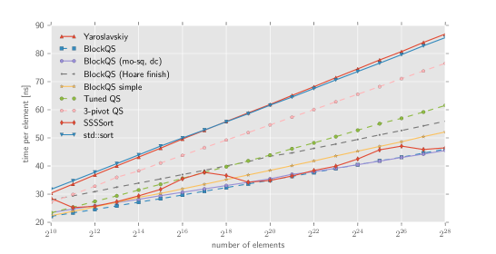
Figure 5. Random permutation of int.

Running Time Experiments

In Figure 5 we present running times on random int permutations of different BlockQuicksort variants and the other algorithms including Katajainen’s Tuned Quicksort and Aumüller and Bingmann’s three-pivot Quicksort. The optimized BlockQuicksort variants need around 45ns per element when sorting $2^{28}$ elements, whereas std::sort needs 85ns per element – thus, there is a speed increase of 88% (i. e. the number of elements sorted per second is increased by 88%).

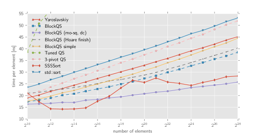
Figure 6. Random int values between $0$ and $\sqrt{n}$.

The same algorithms are displayed in Figure 6 for sorting random ints between $0$ and $\sqrt{n}$. Here, we observe that Tuned Quicksort is much worse than all the other algorithms (already for $n=2^{12}$ it moves outside the displayed range). All variants of BlockQuicksort are faster than std::sort – the duplicate check (dc) version is almost twice as fast.

Figure 7 presents experiments with data containing a lot of duplicates and having specific structures – thus, maybe coming closer to “real-world” inputs (although it is not clear what that means). Since here Tuned Quicksort and three-pivot Quicksort are much slower than all the other algorithms, we exclude these two algorithms from the plots. The array for the left plot contains long already sorted runs. This is most likely the reason that std::sort and Yaroslavskiy’s dual-pivot Quicksort have similar running times to BlockQuicksort (for sorted sequences the conditional branches can be easily predicted what explains the fast running time). The arrays for the middle and right plot start with sorted runs and become more and more erratic; the array for the right one also contains a extremely high number of duplicates. Here the advantage of BlockQuicksort – avoiding conditional branches – can be observed again. In all three plots the check for duplicates (dc) established a considerable improvement.

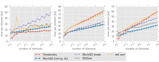
Figure 7. Arrays $A$ of int with duplicates: left: $A[i]=i\mod\left\lfloor\mathinner{\sqrt{n}}\right\rfloor$; middle: $A[i]=i^{2}+n/2\mod n$; right: $A[i]=i^{8}+n/2\mod n$. Since $n$ is always a power of two, the value $n/2$ occurs approximately $n^{7/8}$ times in the last case.

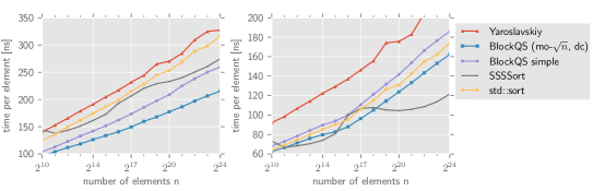
Figure 8. Random permutations – left: Vector; right: Record.

In Figure 8, we show the results of selected algorithms for random permutations of Vector and Record. We conjecture that the good results of Super Scalar Sample Sort on Records are because of its better cache behavior (since Record are large data elements with very cheap comparisons). More running time experiments also on other machines and compiler flags can be found in Appendix A.

More Statistics

Table 1 shows the number of branches taken / branch mispredicted as well as the instruction count and cache misses. Although std::sort has a much lower instruction count than the other algorithms, it induces most branch misses and (except Tuned Quicksort) most L1 cache misses (= L3 refs since no L2 cache is simulated). BlockQuicksort does not only have a low number of branch mispredictions, but also a good cache behavior – one reason for this is that Insertionsort is applied during the recursion and not at the very end.

algorithm	branches taken	branch misses	instructions	L1 refs	L3 refs	L3 misses
std::sort	37.81	10.23	174.82	51.96	1.05	0.41
SSSSort	16.2	3.87	197.06	68.47	0.82	0.5
Yaroslavskiy	52.92	9.51	218.42	59.82	0.79	0.27
BlockQS (mo-$\sqrt{n}$, dc)	20.55	2.39	322.08	89.9	0.77	0.27
BlockQS (mo5-mo5)	20.12	2.31	321.49	88.63	0.78	0.28
BlockQS	20.51	2.25	337.27	92.45	0.88	0.3
BlockQS (no IS)	15.38	1.09	309.85	84.66	0.88	0.3
Tuned QS	29.66	1.44	461.88	105.43	1.23	0.39
Tuned QS (no IS)	24.53	0.26	434.53	97.65	1.22	0.39

Table 1. Instruction count, branch and cache misses when sorting random int permutations of size $16777216=2^{24}$. All displayed numbers are divided by the number of elements.

5. Conclusions and Future Research

We have established an efficient in-place general purpose sorting algorithm, which avoids branch predictions by converting results of comparisons to integers. In the experiments we have seen that it is competitive on different kinds of data. Moreover, in several benchmarks it is almost twice as fast as std::sort. Future research might address the following issues:

• We used Insertionsort as recursion stopper – inducing a linear number of branch misses. Is there a more efficient recursion stopper that induces fewer branch mispredictions?

• More efficient usage of the buffers: in our implementation the buffers on average are not even filled half. To use the space more efficiently one could address the buffers cyclically and scan until one buffer is filled. By doing so, also both buffers could be filled in the same loop – however, with the cost of introducing additional overhead.

• The final rearrangement of the block partitioner is not optimal: for small arrays the similar problems with duplicates arise as for Lomuto’s partitioner.

• Pivot selection strategy: though theoretically optimal, median-of-$\sqrt{n}$ pivot selection is not best in practice. Also we want to emphasize that not only the sample size but also the selection method is important (compare the different behavior of the two versions of std::sort for sorted and reversed permutations). It might be even beneficial to use a fast pseudo-random generator (e. g. a linear congruence generator) for selecting samples for pivot selection.

• Parallel versions: the block structure is very well suited for parallelism.

• A three-pivot version might be interesting, but efficient multi-pivot variants are not trivial: our first attempt was much slower.

Acknowledgments

Thanks to Jyrki Katajainen and Max Stenmark for allowing us to use their Python scripts for measuring branch mispredictions and cache missses and to Lorenz Hübschle-Schneider for his implementation of Super Scalar Sample Sort. We are also indebted to Jan Philipp Wächter for all his help with creating the plots, to Daniel Bahrdt for answering many C++ questions, and to Christoph Greulich for his help with the experiments.

Appendix A More Experimental Results

In Figure 10 and Figure 9 we also included the new GCC implementation of std::sort (GCC version 4.8.4) marked as std::sort (new). The very small difference in the implementation of choosing the second instead of the first element as part of the sample for pivot selection makes a enormous difference when sorting special permutations like decreasingly sorted arrays. This shows how important not only the size of the pivot sample but also the proper selection is. In the other benchmarks both implementations were relatively close, so we do not show both of them.

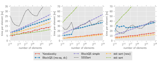
Figure 9. Permutations of int: left: sorted; middle: reversed; right: transposition – $A[i]=i+n/2\mod n$.

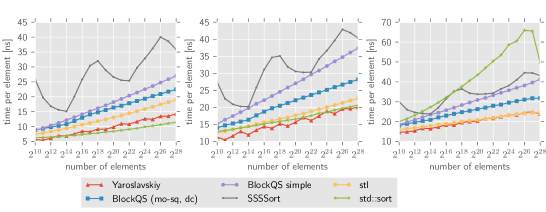
Figure 10. Random permutations of int with at most $k$ inversions ($k$ random swaps of neighboring elements): left: $k=\sqrt{n}$; middle: $k=n$; right: $k=n\log n$.

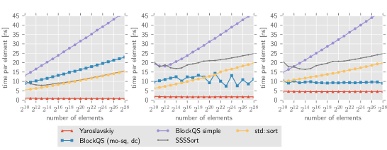
Figure 11. Arrays $A$ of int with many duplicates: Left: constant; middle: $A[i]=0$ for $i<n/2$ and $A[i]=1$ otherwise; right: random 0-1 values.

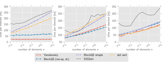
Figure 12. Sorting Vector: Left: random 0-1 values; middle: random values between $0$ and $\sqrt{n}$; right: sorted.

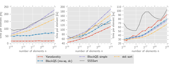
Figure 13. Sorting Record: Left: random 0-1 values; middle: random values between $0$ and $\sqrt{n}$; right: sorted.

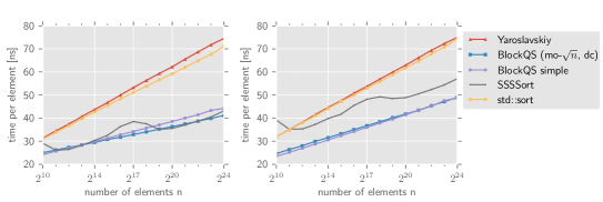
Figure 14. Random permutations of int with other compiler optimizations.
Left: -O3 -march=native -funroll-loops; right: -O1 -march=native.

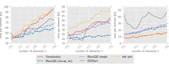
Figure 15. Running time experiments with int on Intel Xeon E5-4627v2 CPU (3.30GHz, 8 cores, 32KB L1 instruction and data cache, 256KB L2 cache per core and 16MB L3 shared cache) with 128GB RAM and operating system Windows Server 2012 R2. We used Cygwin g++ (4.9.3); optimized with flags -O3 -march=native.
Left: random permutation; middle: random values between $0$ and$\sqrt{n}$; right: sorted.

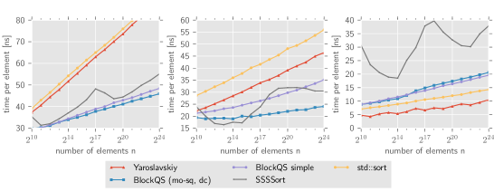
Figure 16. Running time experiments with int on Laptop with Intel Core i7-5500U CPU (2.40GHz, 2 cores, 32KB L1 instruction and data cache, 256KB L2 cache per core and 4MB L3 shared cache) with 8GB RAM and operating system Windows 10. We used Mingw g++ (5.3.0); optimized with flags -O3 -march=native.
Left: random permutation; middle: random values between $0$ and$\sqrt{n}$; right: sorted.

Appendix B C++ Code

Here, we give the C++ code of the basic BlockQuicksort variant (the final rearranging is also in block style, but there is no loop unrolling etc. applied).

⬇

1template<typename iter, typename Compare>

2inline void sort_pair(iter i1, iter i2, Compare less) {

3 typedef typename std::iterator_traits<iter>::value_type T;

4 bool smaller = less(*i2, *i1);

5 T temp = std::move(smaller ? *i1 : temp);

6 *i1 = std::move(smaller ? *i2 : *i1);

7 *i2 = std::move(smaller ? temp : *i2);

8}

9

10template<typename iter, typename Compare>

11inline iter median_of_3(iter i1, iter i2, iter i3, Compare less) {

12 sort_pair(i1, i2, less);

13 sort_pair(i2, i3, less);

14 sort_pair(i1, i2, less);

15 return i2;

16}

17

18template<typename iter, typename Compare>

19inline iter hoare_block_partition_simple(iter begin, iter end, iter pivot_position, Compare less) {

20 typedef typename std::iterator_traits<iter>::difference_type index;

21 index indexL[BLOCKSIZE], indexR[BLOCKSIZE];

22

23 iter last = end - 1;

24 std::iter_swap(pivot_position, last);

25 const typename std::iterator_traits<iter>::value_type & pivot = *last;

26 pivot_position = last;

27 last–;

28

29 int num_left = 0;

30 int num_right = 0;

31 int start_left = 0;

32 int start_right = 0;

33 int num;

34 //main loop

35 while (last - begin + 1 > 2 * BLOCKSIZE)

36 {

37 //Compare and store in buffers

38 if (num_left == 0) {

39 start_left = 0;

40 for (index j = 0; j < BLOCKSIZE; j++) {

41 indexL[num_left] = j;

42 num_left += (!(less(begin[j], pivot)));

43 }

44 }

45 if (num_right == 0) {

46 start_right = 0;

47 for (index j = 0; j < BLOCKSIZE; j++) {

48 indexR[num_right] = j;

49 num_right += !(less(pivot, *(last - j)));

50 }

51 }

52 //rearrange elements

53 num = std::min(num_left, num_right);

54 for (int j = 0; j < num; j++)

55 std::iter_swap(begin + indexL[start_left + j], last - indexR[start_right + j]);

56

57 num_left -= num;

58 num_right -= num;

59 start_left += num;

60 start_right += num;

61 begin += (num_left == 0) ? BLOCKSIZE : 0;

62 last -= (num_right == 0) ? BLOCKSIZE : 0;

63

64 }//end main loop

65

66 //Compare and store in buffers final iteration

67 index shiftR = 0, shiftL = 0;

68 if (num_right == 0 && num_left == 0) { //for small arrays or in the unlikely case that both buffers are empty

69 shiftL = ((last - begin) + 1) / 2;

70 shiftR = (last - begin) + 1 - shiftL;

71 start_left = 0; start_right = 0;

72 for (index j = 0; j < shiftL; j++) {

73 indexL[num_left] = j;

74 num_left += (!less(begin[j], pivot));

75 indexR[num_right] = j;

76 num_right += !less(pivot, *(last - j));

77 }

78 if (shiftL < shiftR)

79 {

80 indexR[num_right] = shiftR - 1;

81 num_right += !less(pivot, *(last - shiftR + 1));

82 }

83 }

84 else if (num_right != 0) {

85 shiftL = (last - begin) - BLOCKSIZE + 1;

86 shiftR = BLOCKSIZE;

87 start_left = 0;

88 for (index j = 0; j < shiftL; j++) {

89 indexL[num_left] = j;

90 num_left += (!less(begin[j], pivot));

91 }

92 }

93 else {

94 shiftL = BLOCKSIZE;

95 shiftR = (last - begin) - BLOCKSIZE + 1;

96 start_right = 0;

97 for (index j = 0; j < shiftR; j++) {

98 indexR[num_right] = j;

99 num_right += !(less(pivot, *(last - j)));

100 }

101 }

102

103 //rearrange final iteration

104 num = std::min(num_left, num_right);

105 for (int j = 0; j < num; j++)

106 std::iter_swap(begin + indexL[start_left + j], last - indexR[start_right + j]);

107

108 num_left -= num;

109 num_right -= num;

110 start_left += num;

111 start_right += num;

112 begin += (num_left == 0) ? shiftL : 0;

113 last -= (num_right == 0) ? shiftR : 0;

114 //end final iteration

115

116

117 //rearrange elements remaining in buffer

118 if (num_left != 0)

119 {

120 int lowerI = start_left + num_left - 1;

121 index upper = last - begin;

122 //search first element to be swapped

123 while (lowerI >= start_left && indexL[lowerI] == upper) {

124 upper–; lowerI–;

125 }

126 while (lowerI >= start_left)

127 std::iter_swap(begin + upper–, begin + indexL[lowerI–]);

128

129 std::iter_swap(pivot_position, begin + upper + 1); // fetch the pivot

130 return begin + upper + 1;

131 }

132 else if (num_right != 0) {

133 int lowerI = start_right + num_right - 1;

134 index upper = last - begin;

135 //search first element to be swapped

136 while (lowerI >= start_right && indexR[lowerI] == upper) {

137 upper–; lowerI–;

138 }

139

140 while (lowerI >= start_right)

141 std::iter_swap(last - upper–, last - indexR[lowerI–]);

142

143 std::iter_swap(pivot_position, last - upper);// fetch the pivot

144 return last - upper;

145 }

146 else { //no remaining elements

147 std::iter_swap(pivot_position, begin);// fetch the pivot

148 return begin;

149 }

150}

151

152template<typename iter, typename Compare>

153struct Hoare_block_partition_simple {

154 static inline iter partition(iter begin, iter end, Compare less) {

155 //choose pivot

156 iter mid = median_of_3(begin, begin + (end - begin) / 2, end, less);

157 //partition

158 return hoare_block_partition_simple(begin + 1, end - 1, mid, less);

159 }

160};

161

162//Quicksort main loop. Implementation based on Tuned Quicksort (Elmasry, Katajainen, Stenmark)

163template<template<class , class> class Partitioner, typename iter, typename Compare>

164inline void qsort(iter begin, iter end, Compare less) {

165 const int depth_limit = 2 * ilogb((double)(end - begin)) + 3;

166 iter stack[80];

167 iter* s = stack;

168 int depth_stack[40];

169 int depth = 0;

170 int* d_s_top = depth_stack;

171 *s = begin;

172 *(s + 1) = end;

173 s += 2;

174 *d_s_top = 0;

175 ++d_s_top;

176 do {

177 if (depth < depth_limit && end - begin > IS_THRESH) {

178 iter pivot = Partitioner< iter, Compare>::partition(begin, end, less);

179 //Push large side to stack and continue on small side

180 if (pivot - begin > end - pivot) {

181 *s = begin;

182 *(s + 1) = pivot;

183 begin = pivot + 1;

184 }

185 else {

186 *s = pivot + 1;

187 *(s + 1) = end;

188 end = pivot;

189 }

190 s += 2;

191 depth++;

192 *d_s_top = depth;

193 ++d_s_top;

194 }

195 else {

196 if (end - begin > IS_THRESH) // if recursion depth limit exceeded

197 std::partial_sort(begin, end, end);

198 else

199 Insertionsort::insertion_sort(begin, end, less); //copy of std::__insertion_sort (GCC 4.7.2)

200

201 //pop new subarray from stack

202 s -= 2;

203 begin = *s;

204 end = *(s + 1);

205 –d_s_top;

206 depth = *d_s_top;

207 }

208 } while (s != stack);

209}

210

211//example invocation of qsort

212int main(void) {

213 std::vector<int> v;

214 //

215 //assign values to v

216 //

217 qsort<Hoare_block_partition_simple>(v.begin(), v.end(), std::less<int>());

218}

References

- [1] ARMv8 Instruction Set Overview, 2011. Document number: PRD03-GENC-010197 15.0.
- [2] Intel 64 and IA-32 Architecture Optimization Reference Manual, 2016. Order Number: 248966-032.
- [3] D. Abhyankar and M. Ingle. Engineering of a quicksort partitioning algorithm. Journal of Global Research in Computer Science, 2(2):17–23, 2011.
- [4] Martin Aumüller and Martin Dietzfelbinger. Optimal partitioning for dual pivot quicksort - (extended abstract). In ICALP, pages 33–44, 2013.
- [5] Martin Aumüller, Martin Dietzfelbinger, and Pascal Klaue. How good is multi-pivot quicksort? CoRR, abs/1510.04676, 2015.
- [6] Paul Biggar, Nicholas Nash, Kevin Williams, and David Gregg. An experimental study of sorting and branch prediction. J. Exp. Algorithmics, 12:1.8:1–39, 2008.
- [7] Gerth Stølting Brodal, Rolf Fagerberg, and Kristoffer Vinther. Engineering a cache-oblivious sorting algorithm. J. Exp. Algorithmics, 12:2.2:1–23, 2008.
- [8] Gerth Stølting Brodal and Gabriel Moruz. Tradeoffs between branch mispredictions and comparisons for sorting algorithms. In WADS, volume 3608 of LNCS, pages 385–395. Springer, 2005.
- [9] Thomas H. Cormen, Charles E. Leiserson, Ronald L. Rivest, and Clifford Stein. Introduction to Algorithms. The MIT Press, 3nd edition, 2009.
- [10] Amr Elmasry and Jyrki Katajainen. Lean programs, branch mispredictions, and sorting. In FUN, volume 7288 of LNCS, pages 119–130. Springer, 2012.
- [11] Amr Elmasry, Jyrki Katajainen, and Max Stenmark. Branch mispredictions don’t affect mergesort. In SEA, pages 160–171, 2012.
- [12] Robert W. Floyd. Algorithm 245: Treesort 3. Comm. of the ACM, 7(12):701, 1964.
- [13] John L. Hennessy and David A. Patterson. Computer Architecture: A Quantitative Approach. Morgan Kaufmann, 5th edition, 2011.
- [14] Charles A. R. Hoare. Quicksort. The Computer Journal, 5(1):10–16, 1962.
- [15] Kanela Kaligosi and Peter Sanders. How branch mispredictions affect quicksort. In ESA, pages 780–791, 2006.
- [16] Jyrki Katajainen. Sorting programs executing fewer branches. CPH STL Report 2263887503, Department of Computer Science, University of Copenhagen, 2014.
- [17] Donald E. Knuth. Sorting and Searching, volume 3 of The Art of Computer Programming. Addison Wesley Longman, 2nd edition, 1998.
- [18] Shrinu Kushagra, Alejandro López-Ortiz, Aurick Qiao, and J. Ian Munro. Multi-pivot quicksort: Theory and experiments. In ALENEX, pages 47–60, 2014.
- [19] Anthony LaMarca and Richard E Ladner. The influence of caches on the performance of sorting. J. Algorithms, 31(1):66–104, 1999.
- [20] Conrado Martínez, Markus E. Nebel, and Sebastian Wild. Analysis of branch misses in quicksort. In Workshop on Analytic Algorithmics and Combinatorics, ANALCO 2015, San Diego, CA, USA, January 4, 2015, pages 114–128, 2015.
- [21] Conrado Martínez and Salvador Roura. Optimal Sampling Strategies in Quicksort and Quickselect. SIAM J. Comput., 31(3):683–705, 2001.
- [22] David R. Musser. Introspective sorting and selection algorithms. Software—Practice and Experience, 27(8):983–993, 1997.
- [23] Charles Price. MIPS IV Instruction Set, 1995.
- [24] Peter Sanders and Sebastian Winkel. Super Scalar Sample Sort. In ESA, pages 784–796, 2004.
- [25] Robert Sedgewick. The analysis of quicksort programs. Acta Inf., 7(4):327–355, 1977.
- [26] Robert Sedgewick. Implementing quicksort programs. Commun. ACM, 21(10):847–857, 1978.
- [27] Sebastian Wild and Markus E. Nebel. Average case analysis of java 7’s dual pivot quicksort. In ESA, pages 825–836, 2012.
- [28] Sebastian Wild, Markus E. Nebel, and Ralph Neininger. Average case and distributional analysis of dual-pivot quicksort. ACM Transactions on Algorithms, 11(3):22:1–42, 2015.
- [29] J. W. J. Williams. Algorithm 232: Heapsort. Communications of the ACM, 7(6):347–348, 1964.
- [30] Vladimir Yaroslavskiy. Dual-Pivot Quicksort algorithm, 2009. URL: http://codeblab.com/wp-content/uploads/2009/09/DualPivotQuicksort.pdf.