Optimal scaling of the Random Walk Metropolis algorithm under $\mathrm{L}^{p}$ mean differentiability

Abstract

This paper considers the optimal scaling problem for high-dimensional random walk Metropolis algorithms for densities which are differentiable in $\mathrm{L}^{p}$ mean but which may be irregular at some points (like the Laplace density for example) and / or are supported on an interval. Our main result is the weak convergence of the Markov chain (appropriately rescaled in time and space) to a Langevin diffusion process as the dimension $d$ goes to infinity. Because the log-density might be non-differentiable, the limiting diffusion could be singular. The scaling limit is established under assumptions which are much weaker than the one used in the original derivation of [6]. This result has important practical implications for the use of random walk Metropolis algorithms in Bayesian frameworks based on sparsity inducing priors.

1 Introduction

A wealth of contributions have been devoted to the study of the behaviour of high-dimensional Markov chains. One of the most powerful approaches for that purpose is the scaling analysis, introduced by [6]. Assume that the target distribution has a density with respect to the $d$-dimensional Lebesgue measure given by:

$$\pi^{d}(x^{d})=\prod_{i=1}^{d}\pi(x_{i}^{d})\,.$$ (1)

The Random Walk Metropolis-Hastings (RWM) updating scheme was first applied in [4] and proceeds as follows. Given the current state $X^{d}_{k}$, a new value $Y_{k+1}^{d}=(Y_{k+1,i}^{d})_{i=1}^{d}$ is obtained by moving independently each coordinate, i.e.  $Y^{d}_{k+1,i}=X^{d}_{k,i}+\ell d^{-1/2}Z_{k+1}^{d}$ where $\ell>0$ is a scaling factor and $\left(Z_{k}\right)_{k\geq 1}$ is a sequence of independent and identically distributed ($\operatorname{i.i.d.}$) Gaussian random variables. Here $\ell$ governs the overall size of the proposed jump and plays a crucial role in determining the efficiency of the algorithm. The proposal is then accepted or rejected according to the acceptance probability $\alpha(X_{k}^{d},Y_{k+1}^{d})$ where $\alpha(x^{d},y^{d})=1\wedge\pi^{d}(y^{d})/\pi^{d}(x^{d})$. If the proposed value is accepted it becomes the next current value, otherwise the current value is left unchanged:

$$X_{k+1}^{d} =X_{k}^{d}+\ell d^{-1/2}Z^{d}_{k+1}\mathds{1}_{\mathcal{A}^{d}_{k+1}}\,,$$ (2)

$$\mathcal{A}_{k+1}^{d} =\left\{U_{k+1}\leq\prod_{i=1}^{d}\pi(X_{k,i}^{d}+\ell d^{-1/2}Z^{d}_{k+1,i})/\pi(X_{k,i}^{d})\right\}\,,$$ (3)

where $\left(U_{k}\right)_{k\geq 1}$ of $\operatorname{i.i.d.}$ uniform random variables on $\left[0,1\right]$ independent of $\left(Z_{k}\right)_{k\geq 1}$.

Under certain regularity assumptions on $\pi$, it has been proved in [6] that if the $X_{0}^{d}$ is distributed under the stationary distribution $\pi^{d}$, then each component of $(X^{d}_{k})_{k\geq 0}$ appropriately rescaled in time converges weakly to a Langevin diffusion process with invariant distribution $\pi$ as $d\to+\infty$.

This result allows to compute the asymptotic mean acceptance rate and to derive a practical rule to tune the factor $\ell$. It is shown in [6] that the speed of the limiting diffusion has a function of $\ell$ has a unique maximum. The corresponding mean acceptance rate in stationarity is equal to $0.234$.

These results have been derived for target distributions of the form (1) where $\pi(x)\propto\exp(-V(x))$ where $V$ is three-times continuously differentiable. Therefore, they do not cover the cases where the target density is continuous but not smooth, for example the Laplace distribution which plays a key role as a sparsity-inducing prior in high-dimensional Bayesian inference.

The aim of this paper is to extend the scaling results for the RWM algorithm introduced in the seminal paper [6, Theorem 3] to densities which are absolutely continuous densities differentiable in $\mathrm{L}^{p}$ mean (DLM) for some $p\geq 2$ but can be either non-differentiable at some points or are supported on an interval. As shown in [3, Section 17.3], differentiability of the square root of the density in $\mathrm{L}^{2}$ norm implies a quadratic approximation property for the log-likelihood known as local asymptotic normality. As shown below, the DLM permits the quadratic expansion of the log-likelihood without paying the twice-differentiability price usually demanded by such a Taylor expansion (such expansion of the log-likelihood plays a key role in [6]).

The paper is organised as follows. In Section 2 the target density $\pi$ is assumed to be positive on $\mathbb{R}$. Theorem 2 proves that under the DLM assumption of this paper, the average acceptance rate and the expected square jump distance are the same as in [6]. Theorem 3 shows that under the same assumptions the rescaled in time Markov chain produced by the RWM algorithm converges weakly to a Langevin diffusion. We show that these results may be applied to a density of the form $\pi(x)\propto\exp(-\lambda\left|x\right|+U(x))$, where $\lambda\geq 0$ and $U$ is a smooth function. In Section 3, we focus on the case where $\pi$ is supported only on an open interval of $\mathbb{R}$. Under appropriate assumptions, Theorem 4 and Theorem 5 show that the same asymptotic results (limiting average acceptance rate and limiting Langevin diffusion associated with $\pi$) hold. We apply our results to Gamma and Beta distributions. The proofs are postponed to Section 4 and Section 5.

2 Positive Target density on $\mathbb{R}$

The key of the proof of our main result will be to show that the acceptance ratio and the expected square jump distance converge to a finite and non trivial limit. In the original proof of [6], the density of the product form (1) with

$$\pi(x)\propto\exp(-V(x))$$ (4)

is three-times continuously differentiable and the acceptance ratio is expanded using the usual pointwise Taylor formula. More precisely, the log-ratio of the density evaluated at the proposed value and at the current state is given by $\sum_{i=1}^{d}\Delta V^{d}_{i}$ where

$$\Delta V^{d}_{i}=V\left(X_{i}^{d}\right)-V\left(X_{i}^{d}+\ell d^{-1/2}Z^{d}_{i}\right)\,,$$ (5)

and where $X^{d}$ is distributed according to $\pi^{d}$ and $Z^{d}$ is a $d$-dimensional standard Gaussian random variable independent of $X$. Heuristically, the two leading terms are $\ell d^{-1/2}\sum_{i=1}^{d}\dot{V}(X^{d}_{i})Z^{d}_{i}$ and $\ell^{2}d^{-1}\sum_{i=1}^{d}\ddot{V}(X^{d}_{i})(Z_{i}^{d})^{2}/2$, where $\dot{V}$ and $\ddot{V}$ are the first and second derivatives of $V$, respectively. By the central limit theorem, this expression converges in distribution to a zero-mean Gaussian random variable with variance $\ell^{2}I$ where

$$I=\int_{\mathbb{R}}\dot{V}^{2}(x)\pi(x)\mathrm{d}x\,.$$ (6)

Note that $I$ is the Fisher information associated with the translation model $\theta\mapsto\pi(x+\theta)$ evaluated at $\theta=0$. Under appropriate technical conditions, the second term converges almost surely to $-\ell^{2}I/2$. Assuming that these limits exist, the acceptance ratio in the RWM algorithm converges to $\mathbb{E}[1\wedge\exp(\mathsf{Z})]$ where $\mathsf{Z}$ is a Gaussian random variable with mean $-\ell^{2}I/2$ and variance $\ell^{2}I$; elementary computations show that $\mathbb{E}[1\wedge\exp(\mathsf{Z})]=2\Phi(-\ell/2\,\sqrt{I})$, where $\Phi$ stands for the cumulative distribution function of a standard normal distribution.

For $t\geq 0$, denote by $Y_{t}^{d}$ the linear interpolation of the Markov chain $(X_{k}^{d})_{k\geq 0}$ after time rescaling:

$$Y_{t}^{d} =\left(\lceil d\,t\rceil-d\,t\right)X_{\left\lfloor d\,t\right\rfloor}^{d}+\left(d\,t-\lfloor d\,t\rfloor\right)X_{\left\lceil d\,t\right\rceil}^{d}$$ (7)

$$=X_{\left\lfloor d\,t\right\rfloor}^{d}+\left(d\,t-\lfloor d\,t\rfloor\right)\ell d^{-1/2}Z^{d}_{\lceil d\,t\rceil}\mathds{1}_{\mathcal{A}^{d}_{\lceil d\,t\rceil}}\,,$$ (8)

where $\lfloor\cdot\rfloor$ and $\lceil\cdot\rceil$ denote the lower and the upper integer part functions. Note that for all $k\geq 0$, $Y_{k/d}^{d}=X_{k}^{d}$. Denote by $(B_{t},t\geq 0)$ the standard Brownian motion.

Theorem 1 ([6]).

Suppose that the target $\pi^{d}$ and the proposal distribution are given by (1)-(4) and (2) respectively. Assume that

1. $V$ is twice continuously differentiable and $\dot{V}$ is Lipshitz continuous ;

2. $\mathbb{E}[(\dot{V}(X))^{8}]<\infty$ and $\mathbb{E}[(\ddot{V}(X))^{4}]<\infty$ where $X$ is distributed according to $\pi$.

Then $(Y_{t,1}^{d},t\geq 0)$, where $Y^{d}_{t,1}$ is the first component of the vector $Y^{d}_{t}$ defined in (7), converges weakly in the Wiener space (equipped with the uniform topology) to the Langevin diffusion

$$\mathrm{d}Y_{t}=\sqrt{h(\ell)}\mathrm{d}B_{t}-\frac{1}{2}h(\ell)\dot{V}(Y_{t})\mathrm{d}t\,,$$ (9)

where $Y_{0}$ is distributed according to $\pi$, $h(\ell)$ is given by

$$h(\ell)=2\ell^{2}\Phi\left(-\frac{\ell}{2}\,\sqrt{I}\right)\,,$$ (10)

and $I$ is defined in (6).

Whereas $V$ is assumed to be twice continuously differentiable, the dual representation of the Fisher information $-\mathbb{E}[\ddot{V}(X)]=\mathbb{E}[(\dot{V}(X))^{2}]=I$ allows us to remove in the statement of the theorem all mention to the second derivative of $V$, which hints that two derivatives might not really be required. For all $\theta,x\in\mathbb{R}$, define

$$\xi_{\theta}(x)=\sqrt{\pi(x+\theta)}\,,$$ (11)

For $p\geq 1$, denote $\left\|f\right\|_{\pi,p}^{p}=\int|f(x)|^{p}\pi(x)\mathrm{d}x$. Consider the following assumptions:

H 1.

There exists a measurable function $\dot{V}:\mathbb{R}\to\mathbb{R}$ such that:

1. There exist $p>4$, $C>0$ and $\beta>1$ such that for all $\theta\in\mathbb{R}$,

   $$\left\|V(\cdot+\theta)-V(\cdot)-\theta\dot{V}(\cdot)\right\|_{\pi,p}\leq C|\theta|^{\beta}\,.$$

2. The function $\dot{V}$ satisfies $\left\|\dot{V}\right\|_{\pi,6}<+\infty$.

Lemma 1.

Assume H 1. Then, the family of densities $\theta\to\pi(\cdot+\theta)$ is Differentiable in Quadratic Mean (DQM) at $\theta=0$ with derivative $\dot{V}$, i.e. there exists $C>0$ such that for all $\theta\in\mathbb{R}$,

$$\left(\int_{\mathbb{R}}\left(\xi_{\theta}(x)-\xi_{0}(x)+\theta\dot{V}(x)\xi_{0}(x)/2\right)^{2}\mathrm{d}x\right)^{1/2}\leq C|\theta|^{\beta}\,,$$

where $\xi_{\theta}$ is given by (11).

Proof.

The proof is postponed to Section 4.1. ∎

The first step in the proof is to show that the acceptance ratio $\mathbb{P}\left(\mathcal{A}_{1}^{d}\right)=\mathbb{E}(1\wedge\exp\{\sum_{i=1}^{d}\Delta V^{d}_{i}\})$, and the expected square jump distance $\mathbb{E}[(Z_{1}^{d})^{2}\{1\wedge\exp(\sum_{i=1}^{d}\Delta V^{d}_{i})\}]$ both converge to a finite value. To that purpose, we consider

$$\mathrm{E}^{d}(q)=\mathbb{E}\left[\left(Z_{1}^{d}\right)^{q}\left|1\wedge\exp\left(\sum_{i=1}^{d}\Delta V^{d}_{i}\right)-1\wedge\exp(\upsilon^{d})\right|\right]\,,$$

where $\Delta V^{d}_{i}$ is given by (5),

$$\upsilon^{d} =-\ell d^{-1/2}Z_{1}^{d}\dot{V}(X_{1}^{d})+\sum_{i=2}^{d}b^{d}(X_{i}^{d},Z_{i}^{d})$$ (12)

$$b^{d}(x,z) =-\frac{\ell z}{\sqrt{d}}\dot{V}(x)+\mathbb{E}\left[2\zeta^{d}(X_{1}^{d},Z_{1}^{d})\right]-\frac{\ell^{2}}{4d}\dot{V}^{2}(x)\,,$$ (13)

$$\zeta^{d}(x,z) =\exp\left\{\left(V\left(x\right)-V\left(x+\ell d^{-1/2}z\right)\right)/2\right\}-1\,.$$ (14)

Proposition 1.

Assume H 1 holds. Let $X^{d}$ be a random variable distributed according to $\pi^{d}$ and $Z^{d}$ be a zero-mean standard Gaussian random variable, independent of $X^{d}$. Then, for any $q\geq 0$, $\lim_{d\to+\infty}\mathrm{E}^{d}(q)=0$.

Proof.

The proof is postponed to Section 4.2. ∎

Proposition 1 shows that it is enough to consider $\upsilon^{d}$ to analyse the asymptotic behaviour of the acceptance ratio and the expected square jump distance as $d\to+\infty$. By the central limit theorem, the term $-\ell\sum_{i=2}^{d}(Z_{i}^{d}/\sqrt{d})\dot{V}(X_{i}^{d})$ in (12) converges in distribution to a zero-mean Gaussian random variable with variance $\ell^{2}I$, where $I$ is defined in (6). By Lemma 4 (Section 4.3), the second term, which is $d\,\mathbb{E}\left[2\zeta^{d}(X_{1}^{d},Z_{1}^{d})\right]=-d\,\mathbb{E}\left[(\zeta^{d}(X^{d}_{1},Z_{1}^{d}))^{2}\right]$ converges to $-\ell^{2}I/4$. The last term converges in probability to $-\ell^{2}I/4$. Therefore, the two last terms plays a similar role in the expansion of the acceptance ratio as the second derivative of $V$ in the regular case.

Theorem 2.

Assume H 1 holds. Then, $\lim_{d\to+\infty}\mathbb{P}\left[\mathcal{A}_{1}^{d}\right]=a(\ell)$, where $a(\ell)=2\Phi(-\sqrt{I}\ell/2)$.

Proof.

The proof is postponed to Section 4.3. ∎

The second result of this paper is that the sequence $\{(Y_{t,1}^{d})_{t\geq 0},d\in\mathbb{N}^{\star}\}$ defined by (7) converges weakly to a Langevin diffusion. Let $(\mu_{d})_{d\geq 1}$ be the sequence of distributions of $\{(Y_{t,1}^{d})_{t\geq 0},d\in\mathbb{N}^{\star}\}$.

Proposition 2.

Assume H 1 holds. Then, the sequence $\left(\mu_{d}\right)_{d\geq 1}$ is tight in $\mathbf{W}$.

Proof.

The proof is adapted from [2]; it is postponed to Section 4.4. ∎

By the Prohorov theorem, the tightness of $\left(\mu_{d}\right)_{d\geq 1}$ implies that this sequence has a weak limit point. We now prove that any limit point is the law of a solution to (9). For that purpose, we use the equivalence between the weak formulation of stochastic differential equations and martingale problems. The generator $\mathrm{L}$ of the Langevin diffusion (9) is given, for all $\phi\in C^{2}_{c}(\mathbb{R},\mathbb{R})$, by

$$\mathrm{L}\phi(x)=\frac{h(\ell)}{2}\left(-\dot{V}(x)\dot{\phi}(x)+\ddot{\phi}(x)\right)\,,$$ (15)

where for $k\in\mathbb{N}$ and $I$ an open subset of $\mathbb{R}$, $C^{k}_{c}(I,\mathbb{R})$ is the space of $k$-times differentiable functions with compact support, endowed with the topology of uniform convergence of all derivatives up to order $k$. We set $C^{\infty}_{c}(I,\mathbb{R})=\bigcap_{k=0}^{\infty}C^{k}_{c}(I,\mathbb{R})$ and $\mathbf{W}=C(\mathbb{R}_{+},\mathbb{R})$. The canonical process is denoted by $(W_{t})_{t\geq 0}$ and $(\mathscr{B}_{t})_{t\geq 0}$ is the associated filtration. For any probability measure $\mu$ on $\mathbf{W}$, the expectation with respect to $\mu$ is denoted by $\mathbb{E}^{\mu}$. A probability measure $\mu$ on $\mathbf{W}$ is said to solve the martingale problem associated with (9) if the pushforward of $\mu$ by $W_{0}$ is $\pi$ and if for all $\phi\in C^{\infty}_{c}(\mathbb{R},\mathbb{R})$, the process

$$\left(\phi(W_{t})-\phi(W_{0})-\int_{0}^{t}\mathrm{L}\phi(W_{u})\mathrm{d}u\right)_{t\geq 0}$$

is a martingale with respect to $\mu$ and the filtration $(\mathscr{B}_{t})_{t\geq 0}$, i.e. if for all $s,t\in\mathbb{R}_{+},s\leq t$,   $\mu\--\mathrm{a.s.}$

$$\mathbb{E}^{\mu}\left[\phi(W_{t})-\phi(W_{0})-\int_{0}^{t}\mathrm{L}\phi(W_{u})\mathrm{d}u\middle|\mathscr{B}_{s}\right]=\phi(W_{s})-\phi(W_{0})-\int_{0}^{s}\mathrm{L}\phi(W_{u})\mathrm{d}s\,.$$

H 2.

The function $\dot{V}$ is continuous on $\mathbb{R}$ except on a Lebesgue-negligible set $\mathcal{D}_{\dot{V}}$ and is bounded on all compact sets of $\mathbb{R}$.

If $\dot{V}$ satisfies H 2, [7, Lemma 1.9, Theorem 20.1 Chapter 5] show that any solution to the martingale problem associated with (9) coincides with the law of a solution to the SDE (9), and conversely. Therefore, uniqueness in law of weak solutions to (9) implies uniqueness of the solution of the martingale problem.

Proposition 3.

Assume H 2 holds. Assume also that for all $\phi\in C_{c}^{\infty}(\mathbb{R},\mathbb{R})$, $m\in\mathbb{N}^{*}$, $g:\mathbb{R}^{m}\to\mathbb{R}$ bounded and continuous, and $0\leq t_{1}\leq\dots\leq t_{m}\leq s\leq t$:

$$\lim_{d\to+\infty}\mathbb{E}^{\mu_{d}}\left[\left(\phi\left(W_{t}\right)-\phi\left(W_{s}\right)-\int_{s}^{t}\mathrm{L}\phi\left(W_{u}\right)\mathrm{d}u\right)g\left(W_{t_{1}},\dots,W_{t_{m}}\right)\right]=0\,.$$ (16)

Then, every limit point of the sequence of probability measures $(\mu_{d})_{d\geq 1}$ on $\mathbf{W}$ is a solution to the martingale problem associated with (9).

Proof.

The proof is postponed to Section 4.5. ∎

Theorem 3.

Assume H 1 and H 2 hold. Assume also that (9) has a unique weak solution. Then, $\left\{(Y_{t,1}^{d})_{t\geq 0},d\in\mathbb{N}^{*}\right\}$ converges weakly to the solution $\left(Y_{t}\right)_{t\geq 0}$ of the Langevin equation defined by (9). Furthermore, $h(\ell)$ is maximized at the unique value of $\ell$ for which $a(\ell)=0.234$, where $a$ is defined in Theorem 2.

Proof.

The proof is postponed to Section 4.6. ∎

Example 1 (Bayesian Lasso).

We apply the results obtained above to a target density $\pi$ on $\mathbb{R}$ given by $x\mapsto\mathrm{e}^{-V(x)}/\int_{\mathbb{R}}\mathrm{e}^{-V(y)}\mathrm{d}y$ where $V$ is given by

$$V:x\mapsto U(x)+\lambda\left|x\right|\,,$$

where $\lambda\geq 0$ and $U$ is twice continuously differentiable with bounded second derivative. Furthermore, $\int_{\mathbb{R}}\left|x\right|^{6}\mathrm{e}^{-V(x)}\mathrm{d}x<+\infty$. Define $\dot{V}:x\mapsto U^{\prime}(x)+\lambda\,\mathrm{sign}(x)$, with $\mathrm{sign}(x)=-1$ if $x\leq 0$ and $\mathrm{sign}(x)=1$ otherwise. We first check that H 1(i) holds. Note that for all $x,y\in\mathbb{R}$,

$$\left|\left|x+y\right|-\left|x\right|-\mathrm{sign}(x)y\right|\leq 2|y|\mathds{1}_{\mathbb{R}_{+}}(\left|y\right|-\left|x\right|)\,,$$ (17)

which implies that, for any $p\geq 1$, there exists $C_{p}$ such that

$$\left\|V(\cdot+\theta)-V(\cdot)-\theta\dot{V}(\cdot)\right\|_{\pi,p} \leq\left\|U(\cdot+\theta)-U(\cdot)-\theta U^{\prime}(\cdot)\right\|_{\pi,p}+\lambda\left\|\left|\cdot+\theta\right|-\left|\cdot\right|-\theta\,\mathrm{sign}(\cdot)\right\|_{\pi,p}$$

$$\leq\left\|U^{\prime\prime}\right\|_{\infty}\,\theta^{2}+2\,\left|\theta\right|\lambda\{\pi(\left[-\theta,\theta\right])\}^{1/p}\leq C\left|\theta\right|^{p+1/p}\vee\left|\theta\right|^{2}\,.$$

Assumptions H 1(ii) and H 2 are easy to check. The uniqueness in law of (9) is established in [1, Theorem 4.5 (i)]. Therefore, Theorem 3 can be applied.

3 Target density supported on an interval of $\mathbb{R}$

We now extend our results to densities supported by a open interval $\mathcal{I}\subset\mathbb{R}$ :

$$\pi(x)\propto\exp(-V(x))\mathds{1}_{\mathcal{I}}(x)\,,$$

where $V:\mathcal{I}\to\mathbb{R}$ is a measurable function. Note that by convention $V(x)=-\infty$ for all $x\notin\mathcal{I}$. Denote by $\overline{\mathcal{I}}$ the closure of $\mathcal{I}$ in $\mathbb{R}$. The results of Section 2 cannot be directly used in such a case, as $\pi$ is no longer positive on $\mathbb{R}$. Consider the following assumption.

G 1.

There exists a measurable function $\dot{V}:\mathcal{I}\to\mathbb{R}$ and $\mathrm{r}>1$ such that:

1. There exist $p>4$, $C>0$ and $\beta>1$ such that for all $\theta\in\mathbb{R}$,

   $$\left\|\{V(\cdot+\theta)-V(\cdot)\}\mathds{1}_{\mathcal{I}}(\cdot+\mathrm{r}\theta)\mathds{1}_{\mathcal{I}}(\cdot+(1-\mathrm{r})\theta)-\theta\dot{V}(\cdot)\right\|_{\pi,p}\leq C|\theta|^{\beta}\,,$$

   with the convention $0\times\infty=0$.

2. The function $\dot{V}$ satisfies $\|\dot{V}\|_{\pi,6}<+\infty$.

3. There exist $\gamma\geq 6$ and $C>0$ such that, for all $\theta\in\mathbb{R}$,

   $$\int_{\mathbb{R}}\mathds{1}_{\mathcal{I}^{c}}(x+\theta)\pi(x)\mathrm{d}x\leq C|\theta|^{\gamma}\,.$$

As an important consequence of G 1(iii), if $X$ is distributed according to $\pi$ and is independent of the standard random variable $Z$, there exists a constant $C$ such that

$$\mathbb{P}\left(X+\ell d^{-1/2}Z\in\mathcal{I}^{c}\right)\leq Cd^{-\gamma/2}\,.$$ (18)

Theorem 4.

Assume G 1 holds. Then, $\lim_{d\to+\infty}\mathbb{P}\left[\mathcal{A}_{1}^{d}\right]=a(\ell)$, where $a(\ell)=2\Phi(-\sqrt{I}\ell/2)$.

Proof.

The proof is postponed to Section 5.1. ∎

We now established the weak convergence of the sequence $\{(Y_{t,1}^{d})_{t\geq 0},d\in\mathbb{N}^{\star}\}$, following the same steps as for the proof of Theorem 3. Denote for all $d\geq 1$, $\mu_{d}$ the law of the process $(Y_{t,1}^{d})_{t\geq 0}$.

Proposition 4.

Assume G 1 holds. Then, the sequence $\left(\mu_{d}\right)_{d\geq 1}$ is tight in $\mathbf{W}$.

Proof.

The proof is postponed to Section 5.2. ∎

Contrary to the case where $\pi$ is positive on $\mathbb{R}$, we do not assume that $\dot{V}$ is bounded on all compact sets of $\mathbb{R}$. Therefore, we consider the local martingale problem associated with (9): with the notations of Section 2, a probability measure $\mu$ on $\mathbf{W}$ is said to solve the local martingale problem associated with (9) if the pushforward of $\mu$ by $W_{0}$ is $\pi$ and if for all $\psi\in C^{\infty}(\mathbb{R},\mathbb{R})$, the process

$$\left(\psi(W_{t})-\psi(W_{0})-\int_{0}^{t}\mathrm{L}\psi(W_{u})\mathrm{d}u\right)_{t\geq 0}$$

is a local martingale with respect to $\mu$ and the filtration $(\mathscr{B}_{t})_{t\geq 0}$. By [1, Theorem 1.27], any solution to the local martingale problem associated with (9) coincides with the law of a solution to the SDE (9) and conversely. If (9) admits a unique solution in law, this law is the unique solution to the local martingale problem associated with (9). We first prove that any limit point $\mu$ of $(\mu_{d})_{d\geq 1}$ is a solution to the local martingale problem associated with (9).

G 2.

The function $\dot{V}$ is continuous on $\mathcal{I}$ except on a null-set $\mathcal{D}_{\dot{V}}$, with respect to the Lebesgue measure, and is bounded on all compact sets of $\mathcal{I}$.

This condition does not preclude that $\dot{V}$ is unbounded at the boundary of $\mathcal{I}$.

Proposition 5.

Assume G 1 and G 2 hold. Assume also that for all $\phi\in C_{c}^{\infty}(\mathcal{I},\mathbb{R})$, $m\in\mathbb{N}^{*}$, $g:\mathbb{R}^{m}\to\mathbb{R}$ bounded and continuous, and $0\leq t_{1}\leq\dots\leq t_{m}\leq s\leq t$:

$$\lim_{d\to+\infty}\mathbb{E}^{\mu_{d}}\left[\left(\phi\left(W_{t}\right)-\phi\left(W_{s}\right)-\int_{s}^{t}\mathrm{L}\phi\left(W_{u}\right)\mathrm{d}u\right)g\left(W_{t_{1}},\dots,W_{t_{m}}\right)\right]=0\,.$$ (19)

Then, every limit point of the sequence of probability measures $(\mu_{d})_{d\geq 1}$ on $\mathbf{W}$ is a solution to the local martingale problem associated with (9).

Proof.

The proof is postponed to Section 5.3. ∎

Theorem 5.

Assume G 1 and G 2 hold. Assume also that (9) has a unique weak solution. Then, $\left\{(Y_{t,1}^{d})_{t\geq 0},d\in\mathbb{N}^{*}\right\}$ converges weakly to the solution $\left(Y_{t}\right)_{t\geq 0}$ of the Langevin equation defined by (9). Furthermore, $h(\ell)$ is maximized at the unique value of $\ell$ for which $a(\ell)=0.234$, where $a$ is defined in Theorem 2.

Proof.

The proof is along the same lines as the proof of Theorem 3 and is postponed to Section 5.4. ∎

The conditions for uniqueness in law of singular one-dimensional stochastic differential equations are given in [1]. These conditions are rather involved and difficult to summarize in full generality. We rather illustrate Theorem 5 by two examples.

Example 2 (Application to the Gamma distribution).

Define the class of the generalized Gamma distributions as the family of densities on $\mathbb{R}$ given by

$$\pi_{\upgamma}:x\mapsto x^{\mathrm{a}_{1}-1}\exp(-x^{\mathrm{a}_{2}})\mathds{1}_{\mathbb{R}_{+}^{\star}}(x)\Big{/}\int_{\mathbb{R}_{+}^{\star}}y^{\mathrm{a}_{1}-1}\exp(-y^{\mathrm{a}_{2}})\mathrm{d}y\,,$$

with two parameters $\mathrm{a}_{1}>6$ and $\mathrm{a}_{2}>0$. Note that in this case $\mathcal{I}=\mathbb{R}_{+}^{\star}$, for all $x\in\mathcal{I}$, $V_{\upgamma}:x\mapsto x^{\mathrm{a}_{2}}-(\mathrm{a}_{1}-1)\log x$ and $\dot{V}_{\upgamma}:x\mapsto\mathrm{a}_{2}x^{\mathrm{a}_{2}-1}-(\mathrm{a}_{1}-1)/x$. We check that G 1 holds with $\mathrm{r}=3/2$. First, we show that G 1(i) holds with $p=5$. Write for all $\theta\in\mathbb{R}$ and $x\in\mathcal{I}$,

$$\left\{V_{\upgamma}(x+\theta)-V_{\upgamma}(x)\right\}\mathds{1}_{\mathcal{I}}(x+(1-r)\theta)\mathds{1}_{\mathcal{I}}(x+r\theta)-\theta\dot{V}_{\upgamma}(x)=\mathcal{E}_{1}+\mathcal{E}_{2}+\mathcal{E}_{3}\,,$$

where

$$\mathcal{E}_{1} =\theta\dot{V}_{\upgamma}(x)\left\{\mathds{1}_{\mathcal{I}}(x-\theta/2)\mathds{1}_{\mathcal{I}}(x+3\theta/2)-1\right\}\,,$$

$$\mathcal{E}_{2} =(1-\mathrm{a}_{1})\left\{\log(1+\theta/x)-\theta/x\right\}\mathds{1}_{\mathcal{I}}(x-\theta/2)\mathds{1}_{\mathcal{I}}(x+3\theta/2)\,,$$

$$\mathcal{E}_{3} =((x+\theta)^{\mathrm{a}_{2}}-x^{\mathrm{a}_{2}}-\mathrm{a}_{2}\theta x^{\mathrm{a}_{2}-1})\mathds{1}_{\mathcal{I}}(x-\theta/2)\mathds{1}_{\mathcal{I}}(x+3\theta/2)\,.$$

It is enough to prove that there exists $q>5$ such that for all $i\in\{1,2,3\}$, $\int_{\mathcal{I}}\left|\mathcal{E}_{i}\right|^{5}\pi_{\upgamma}(x)\mathrm{d}x\leq C|\theta|^{q}$. The result is proved for $\theta<0$ (the proof for $\theta>0$ follows the same lines). For all $\theta\in\mathbb{R}$ using $\mathrm{a}_{1}>6$,

$$\int_{\mathbb{R}^{*}_{+}}\left|\mathcal{E}_{1}\right|^{5}\pi_{\upgamma}(x)\mathrm{d}x \leq C|\theta|^{5}\int_{0}^{3|\theta|/2}\left\{1/x^{5}+x^{5(\mathrm{a}_{2}-1)}\right\}x^{\mathrm{a}_{1}-1}\mathrm{e}^{-x^{\mathrm{a}_{2}}}\mathrm{d}x\,,$$

$$\leq C|\theta|^{\mathrm{a}_{1}}\left(\int_{0}^{3/2}x^{\mathrm{a}_{1}-6}\mathrm{e}^{-(|\theta|x)^{\mathrm{a}_{2}}}\mathrm{d}x+|\theta|^{5\mathrm{a}_{2}}\int_{0}^{3/2}x^{5(\mathrm{a}_{2}-1)+\mathrm{a}_{1}-1}\mathrm{e}^{-(|\theta|x)^{\mathrm{a}_{2}}}\mathrm{d}x\right)\,,$$

$$\leq C(|\theta|^{\mathrm{a}_{1}}+|\theta|^{5\mathrm{a}_{2}+\mathrm{a}_{1}})\,.$$ (20)

On the other hand, as for all $x>-1$, $x/(x+1)\leq\log(1+x)\leq x$, for all $\theta<0$, and $x\geq 3|\theta|/2$,

$$\left|\log(1+\theta/x)-\theta/x\right|\leq\frac{|\theta|^{2}}{x^{2}(1+\theta/x)}\leq 3|\theta|^{2}/x^{2}\,,$$

where the last inequality come from $|\theta|/x\leq 2/3$. Then, it yields

$$\int_{\mathbb{R}^{*}_{+}}\left|\mathcal{E}_{2}(x)\right|^{5}\pi_{\upgamma}(x)\mathrm{d}x \leq C|\theta|^{10}\left(\int_{3|\theta|/2}^{1}x^{\mathrm{a}_{1}-11}\mathrm{e}^{-x^{\mathrm{a}_{2}}}\mathrm{d}x+\int_{1}^{+\infty}x^{\mathrm{a}_{1}-11}\mathrm{e}^{-x^{\mathrm{a}_{2}}}\mathrm{d}x\right)\,,$$

$$\leq C(|\theta|^{\mathrm{a}_{1}}+|\theta|^{10})\,.$$ (21)

For the last term, for all $\theta<0$ and all $x\geq 3|\theta|/2$, using a Taylor expansion of $x\mapsto x^{\mathrm{a}_{2}}$, there exists $\zeta\in[x+\theta,x]$ such that

$$\left|(x+\theta)^{\mathrm{a}_{2}}-x^{\mathrm{a}_{2}}-\mathrm{a}_{2}\theta x^{\mathrm{a}_{2}-1}\right|\leq C|\theta|^{2}|\zeta|^{\mathrm{a}_{2}-2}\leq C|\theta|^{2}\left|x\right|^{\mathrm{a}_{2}-2}\,.$$

Then,

$$\int_{\mathbb{R}^{*}_{+}}\left|\mathcal{E}_{3}(x)\right|^{5}\pi_{\upgamma}(x)\mathrm{d}x\leq C|\theta|^{10}\int_{3|\theta|/2}^{+\infty}x^{5(\mathrm{a}_{2}-2)+\mathrm{a}_{1}-1}\mathrm{e}^{-x^{\mathrm{a}_{2}}}\mathrm{d}x\leq C(|\theta|^{5\mathrm{a}_{2}+\mathrm{a}_{1}}+|\theta|^{10})\,.$$ (22)

Combining (20), (21),(22) and using that $\mathrm{a}_{1}>6$ concludes the proof of G 1(i) for $p=5$. The proof of G 1(ii) follows from

$$\int_{\mathbb{R}^{*}_{+}}|\dot{V}_{\upgamma}(x)|^{6}\pi_{\upgamma}(x)\mathrm{d}x \leq C\left(\int_{\mathbb{R}^{*}_{+}}x^{\mathrm{a}_{1}-1+6(\mathrm{a}_{2}-1)}\mathrm{e}^{-x^{\mathrm{a}_{2}}}\mathrm{d}x+\int_{\mathbb{R}^{*}_{+}}x^{\mathrm{a}_{1}-7}\mathrm{e}^{-x^{\mathrm{a}_{2}}}\mathrm{d}x\right)<\infty$$

and G 1(iii) follows from $\int_{\mathbb{R}}\mathds{1}_{\mathcal{I}^{c}}(x+\theta)\pi_{\upgamma}(x)\mathrm{d}x\leq C|\theta|^{\mathrm{a}_{1}}$. Now consider the Langevin equation associated with $\pi_{\upgamma}$ given by $\mathrm{d}Y_{t}=-\dot{V}_{\upgamma}(Y_{t})\mathrm{d}t+\sqrt{2}\mathrm{d}B_{t}$ with initial distribution $\pi_{\upgamma}$. This stochastic differential equation has $0$ as singular point, which has right type $3$ according to the terminology of [1]. On the other hand $\infty$ has type $A$ and the existence and uniqueness in law for the SDE follows from [1, Theorem 4.6 (viii)]. Since G 2 is straightforward, Theorem 5 can be applied.

Example 3 (Application to the Beta distribution).

Consider now the case of the Beta distributions $\pi_{\upbeta}$ with density $x\mapsto x^{a_{1}-1}(1-x)^{a_{2}-1}\mathds{1}_{\left(0,1\right)}(x)$ with $a_{1},a_{2}>6$. Here $\mathcal{I}=\left(0,1\right)$ and the log-density $V_{\upbeta}$ and its derivative on $\mathcal{I}$ are defined by $V_{\upbeta}(x)=-(a_{1}-1)\log x-(a_{2}-1)\log(1-x)$ and $\dot{V}_{\upbeta}(x)=-(a_{1}-1)/x-(a_{2}-1)/(1-x)$. Along the same lines as above, $\pi_{\upbeta}$ satisfies G 1 and G 2. Hence Theorem 4 can be applied if we establish the uniqueness in law for the Langevin equation associated with $\pi_{\upbeta}$ defined by $\mathrm{d}Y_{t}=-\dot{V}_{\upbeta}(Y_{t})\mathrm{d}t+\sqrt{2}\mathrm{d}B_{t}$ with initial distribution $\pi_{\upbeta}$. In the terminology of [1], $0$ has right type $3$ and $1$ has left type $3$. Therefore by [1, Theorem 2.16 (i), (ii)], the SDE has a global unique weak solution. To illustrate our findings, consider the Beta distribution with parameters $a_{1}=10$ and $a_{2}=10$. Define the expected square distance by $\operatorname{ESJD}^{d}(\ell)=\mathbb{E}\left[\left\|X_{1}^{d}-X_{0}^{d}\right\|^{2}\right]$ where $X_{0}^{d}$ has distribution $\pi_{\upbeta}^{d}$ and $X_{1}^{d}$ is the first iterate of the Markov chain defined by the Random Walk Metropolis algorithm given in (2). By Theorem 4 and Theorem 5, we have $\lim_{d\to+\infty}\operatorname{ESJD}^{d}(\ell)=h(\ell)=\ell^{2}a(\ell)$. Figure 1 displays an empirical estimation for the $\operatorname{ESJD}^{d}$ for dimensions $d=10,50,100$ as a function of the empirical mean acceptance rate. We can observe that as expected, the $\operatorname{ESJD}^{d}$ converges to some limit function as $d$ goes infinity, and this function has a maximum for a mean acceptance probability around $0.23$.

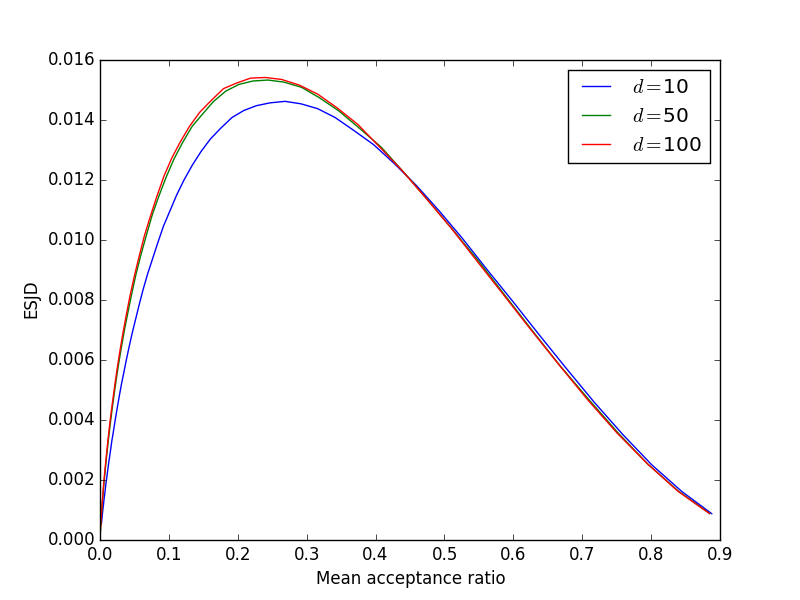
Figure 1: Expected square jumped distance for the beta distribution with parameters $a_{1}=10$ and $a_{2}=10$ as a function of the mean acceptance rate for $d=10,50,100$.

4 Proofs of Section 2

For any real random variable $Y$ and any $p\geq 1$, let $\left\|Y\right\|_{p}:=\mathbb{E}[|Y|^{p}]^{1/p}$.

4.1 Proof of Lemma 1

Let $\Delta_{\theta}V(x)=V(x)-V(x+\theta)$. By definition of $\xi_{\theta}$ and $\pi$,

$$\left(\xi_{\theta}(x)-\xi_{0}(x)+\theta\dot{V}(x)\xi_{0}(x)/2\right)^{2}\leq 2\left\{A_{\theta}(x)+B_{\theta}(x)\right\}\pi(x)\,,$$

where

$$A_{\theta}(x)=\left(\exp(\Delta_{\theta}V(x)/2)-1-\Delta_{\theta}V(x)/2\right)^{2}\,,$$

$$B_{\theta}(x)=\left(\Delta_{\theta}V(x)+\theta\dot{V}(x)\right)^{2}/4.$$

By H 1(i), $\left\|B_{\theta}\right\|_{\pi,p}\leq C|\theta|^{\beta}$. For $A_{\theta}$, note that for all $x\in\mathbb{R}$, $(\exp(x)-1-x)^{2}\leq 2x^{4}(\exp(2x)+1)$. Then,

$$\int_{\mathbb{R}}A_{\theta}(x)\pi(x)\mathrm{d}x \leq C\int_{\mathbb{R}}\Delta_{\theta}V(x)^{4}\left(1+\mathrm{e}^{\Delta_{\theta}V(x)}\right)\pi(x)\mathrm{d}x$$

$$\leq C\int_{\mathbb{R}}\left(\Delta_{\theta}V(x)^{4}+\Delta_{-\theta}V(x)^{4}\right)\pi(x)\mathrm{d}x\,.$$

The proof is completed writing (the same inequality holds for $\Delta_{-\theta}V$):

$$\int_{\mathbb{R}}\Delta_{\theta}V(x)^{4}\pi(x)\mathrm{d}x\leq C\left[\int_{\mathbb{R}}\left(\Delta_{\theta}V(x)-\theta\dot{V}(x)\right)^{4}\pi(x)\mathrm{d}x+\theta^{4}\int_{\mathbb{R}}\dot{V}^{4}(x)\pi(x)\mathrm{d}x\right]$$

and using H 1(i)-(ii).

4.2 Proof of Proposition 1

Define

$$R(x)=\int_{0}^{x}\frac{(x-u)^{2}}{(1+u)^{3}}\mathrm{d}u\,.$$ (23)

$R$ is the remainder term of the Taylor expansion of $x\mapsto\log(1+x)$:

$$\log(1+x)=x-x^{2}/2+R(x)\,.$$ (24)

We preface the proof by the following Lemma.

Lemma 2.

Assume H 1 holds. Then, if $X$ is a random variable distributed according to $\pi$ and $Z$ is a standard Gaussian random variable independent of $X$,

1. $\lim_{d\to+\infty}d\ \left\|\zeta^{d}(X,Z)+\ell Z\dot{V}(X)/(2\sqrt{d})\right\|_{2}^{2}=0$.

2. $\lim_{d\to+\infty}\sqrt{d}\left\|V(X)-V(X+\ell Z/\sqrt{d})+\ell Z\dot{V}(X)/\sqrt{d}\right\|_{p}=0.$

3. $\lim_{d\to\infty}d\left\|R\left(\zeta^{d}(X,Z)\right)\right\|_{1}=0$,

where $\zeta^{d}$ is given by (14).

Proof.

Using the definitions (11) and (14) of $\zeta^{d}$ and $\xi_{\theta}$ ,

$$\zeta^{d}(x,z)=\xi_{\ell zd^{-1/2}}(x)/\xi_{0}(x)-1\,.$$ (25)

1. The proof follows from Lemma 1 using that $\beta>1$:

   $$\left\|\zeta^{d}(X,Z)+\ell Z\dot{V}(X)/(2\sqrt{d})\right\|_{2}^{2}\leq C\ell^{2\beta}d^{-\beta}\mathbb{E}\left[|Z|^{2\beta}\right]\,.$$

2. Using H 1(i), we get that

   $$\left\|V(X)-V(X+\ell Z/\sqrt{d})+\ell Z\dot{V}(X)/\sqrt{d}\right\|_{p}^{p}\leq C\ell^{\beta p}d^{-\beta p/2}\mathbb{E}\left[\left|Z\right|^{\beta p}\right]$$

   and the proof follows since $\beta>1$.

3. Note that for all $x>0$, $u\in\left[0,x\right]$, $|(x-u)(1+u)^{-1}|\leq\left|x\right|$, and the same inequality holds for $x\in\left(-1,0\right]$ and $u\in\left[x,0\right]$. Then by (23) and (24), for all $x>-1$, $\left|R(x)\right|\leq x^{2}\left|\log(1+x)\right|$.

   Then by (50), setting $\Psi_{d}(x,z)=R(\zeta^{d}(x,z))$

   $$\left|\Psi_{d}(x,z)\right|\leq\left(\xi_{\ell zd^{-1/2}}(x)/\xi_{0}(x)-1\right)^{2}\left|V(x+\ell zd^{-1/2})-V(x)\right|/2\,.$$

   Since for all $x\in\mathbb{R}$, $|\exp(x)-1|\leq|x|(\exp(x)+1)$, this yields,

   $$\left|\Psi_{d}(x,z)\right|\leq 4^{-1}\left|V(x+\ell zd^{-1/2})-V(x)\right|^{3}\left(\exp\left(V(x)-V(x+\ell zd^{-1/2})\right)+1\right)\,,$$

   which implies that

   $$\int_{\mathbb{R}}\left|\Psi_{d}(x,z)\right|\pi(x)\mathrm{d}x\leq 4^{-1}\int_{\mathbb{R}}\left|V(x+\ell zd^{-1/2})-V(x)\right|^{3}\{\pi(x)+\pi(x+\ell zd^{-1/2})\}\mathrm{d}x\,.$$

   By Hölder’s inequality and using H 1(i),

   $$\int_{\mathbb{R}}\left|\Psi_{d}(x,z)\right|\pi(x)\mathrm{d}x\leq C\left(\left|\ell zd^{-1/2}\right|^{3}\left(\int_{\mathbb{R}}\left|\dot{V}(x)\right|^{4}\pi(x)\mathrm{d}x\right)^{3/4}+\left|\ell zd^{-1/2}\right|^{3\beta}\right)\,.$$

   The proof follows from H 1(ii) since $\beta>1$.

∎

For all $d\geq 1$, let $X^{d}$ be distributed according to $\pi^{d}$, and $Z^{d}$ be $d$-dimensional Gaussian random variable independent of $X^{d}$, set

$$\mathrm{J}^{d}=\left\|\sum_{i=2}^{d}\left\{\Delta V^{d}_{i}-b^{d}(X_{i}^{d},Z_{i}^{d})\right\}\right\|_{1}\,,$$

where $\Delta V^{d}_{i}$ and $b^{d}$ are defined in (5) and (13), respectively.

Lemma 3.

$\lim_{d\to+\infty}\mathrm{J}^{d}=0$.

Proof.

Noting that $\Delta V^{d}_{i}=2\log\left(1+\zeta^{d}\left(X_{i}^{d},Z_{i}^{d}\right)\right)$ and using (24), we get

$$\mathrm{J}^{d}\leq\sum_{i=1}^{3}\mathrm{J}_{i}^{d}=\left\|\sum_{i=2}^{d}2\zeta^{d}\left(X_{i}^{d},Z_{i}^{d}\right)+\frac{\ell Z_{i}^{d}}{\sqrt{d}}\dot{V}(X_{i}^{d})-\mathbb{E}\left[2\zeta^{d}(X_{i}^{d},Z_{i}^{d})\right]\right\|_{1}\\ +\left\|\sum_{i=2}^{d}\zeta^{d}\left(X_{i}^{d},Z_{i}^{d}\right)^{2}-\frac{\ell^{2}}{4d}\dot{V}^{2}(X_{i}^{d})\right\|_{1}+2\left\|\sum_{i=2}^{d}R\left(\zeta^{d}\left(X_{i}^{d},Z_{i}^{d}\right)\right)\right\|_{1}\,,$$

where $R$ is defined by (23). By Lemma 2(i), the first term goes to $0$ as $d$ goes to $+\infty$ since

$$\mathrm{J}_{1}^{d}\leq\sqrt{d}\,\left\|2\zeta^{d}\left(X_{1}^{d},Z_{1}^{d}\right)+\frac{\ell Z_{1}^{d}}{\sqrt{d}}\dot{V}(X_{1}^{d})\right\|_{2}\,.$$

Consider now $\mathrm{J}_{2}^{d}$. We use the following decomposition for all $2\leq i\leq d$,

$$\zeta^{d}(X_{i}^{d},Z_{i}^{d})^{2}-\frac{\ell^{2}}{4d}\dot{V}^{2}(X_{i}^{d})=\left(\zeta^{d}(X_{i}^{d},Z_{i}^{d})+\frac{\ell}{2\sqrt{d}}Z_{i}^{d}\dot{V}(X_{i}^{d})\right)^{2}\\ -\frac{\ell}{\sqrt{d}}Z_{i}^{d}\dot{V}(X_{i}^{d})\left(\zeta^{d}(X_{i}^{d},Z_{i}^{d})+\frac{\ell}{2\sqrt{d}}Z_{i}^{d}\dot{V}(X_{i}^{d})\right)+\frac{\ell^{2}}{4d}\left\{(Z_{i}^{d})^{2}-1\right\}\dot{V}^{2}(X_{i}^{d})\,.$$

Then,

$$\mathrm{J}^{d}_{2}\leq d\,\left\|\zeta^{d}(X_{1}^{d},Z_{1}^{d})+\frac{\ell}{2\sqrt{d}}Z_{1}^{d}\dot{V}(X_{1}^{d})\right\|_{2}^{2}+\frac{\ell^{2}}{4d}\,\left\|\sum_{i=2}^{d}\dot{V}^{2}(X_{i}^{d})\left\{(Z_{i}^{d})^{2}-1\right\}\right\|_{1}\\ +\ell\sqrt{d}\,\left\|\dot{V}(X_{1}^{d})Z_{1}^{d}\left(\zeta^{d}(X_{1}^{d},Z_{1}^{d})+\frac{\ell}{2\sqrt{d}}Z_{1}^{d}\dot{V}(X_{1}^{d})\right)\right\|_{1}\,.$$

Using H 1(ii), Lemma 2(i) and the Cauchy-Schwarz inequality show that the first and the last term converge to zero. For the second term note that $\mathbb{E}\left[(Z_{i}^{d})^{2}-1\right]=0$ so that

$$d^{-1}\left\|\sum_{i=2}^{d}\dot{V}^{2}(X_{i}^{d})\left\{(Z_{i}^{d})^{2}-1\right\}\right\|_{1}\leq d^{-1/2}\,\mathrm{Var}\left[\dot{V}^{2}(X_{1}^{d})\left\{(Z_{1}^{d})^{2}-1\right\}\right]^{1/2}\to 0\,.$$

Finally, $\lim_{d\to\infty}\mathrm{J}_{3}^{d}=0$ by (24) and Lemma 2(iii). ∎

Proof of Proposition 1.

Let $q>0$ and $\Lambda^{d}=-\ell d^{-1/2}Z_{1}^{d}\dot{V}(X_{1}^{d})+\sum_{i=2}^{d}\Delta V^{d}_{i}$. By the triangle inequality, $\mathrm{E}^{d}(q)\leq\mathrm{E}^{d}_{1}(q)+\mathrm{E}^{d}_{2}(q)$ where

$$\mathrm{E}^{d}_{1}(q) =\mathbb{E}\left[\left(Z_{1}^{d}\right)^{q}\left|1\wedge\exp\left\{\sum_{i=1}^{d}\Delta V^{d}_{i}\right\}-1\wedge\exp\left\{\Lambda^{d}\right\}\right|\right]\,,$$

$$\mathrm{E}^{d}_{2}(q) =\mathbb{E}\left[\left(Z_{1}^{d}\right)^{q}\left|1\wedge\exp\left\{\Lambda^{d}\right\}-1\wedge\exp\left\{\upsilon^{d}\right\}\right|\right]\,.$$

Since $t\mapsto 1\wedge\mathrm{e}^{t}$ is $1$-Lipschitz, by the Cauchy-Schwarz inequality we get

$$\mathrm{E}^{d}_{1}(q)\leq\left\|Z_{1}^{d}\right\|_{2q}^{q}\left\|\Delta V^{d}_{1}+\ell d^{-1/2}Z_{1}^{d}\dot{V}(X_{1}^{d})\right\|_{2}\,.$$

By Lemma 2(ii), $\mathrm{E}^{d}_{1}(q)$ goes to $0$ as $d$ goes to $+\infty$. Consider now $\mathrm{E}^{d}_{2}(q)$. Using again that $t\mapsto 1\wedge\mathrm{e}^{t}$ is $1$-Lipschitz and Lemma 3, $\mathrm{E}^{d}_{2}(q)$ goes to $0$. ∎

4.3 Proof of Theorem 2

Following [2], we introduce the function $\mathcal{G}$ defined on $\overline{\mathbb{R}}_{+}\times\mathbb{R}$ by:

$$\mathcal{G}(a,b)=\left\{\begin{array}[]{ll}\mathrm{exp}\left(\frac{a-b}{2}\right)\Phi\left(\frac{b}{2\sqrt{a}}-\sqrt{a}\right)&\mbox{if}\;a\in(0,+\infty)\,,\\ 0&\mbox{if}\;a=+\infty\,,\\ \mathrm{exp}\left(-\frac{b}{2}\right)\mathds{1}_{\left\{b>0\right\}}&\mbox{if}\;a=0\,,\end{array}\right.$$ (26)

where $\Phi$ is the cumulative distribution function of a standard normal variable, and $\Gamma$:

$$\Gamma(a,b)=\left\{\begin{array}[]{ll}\Phi\left(-\frac{b}{2\sqrt{a}}\right)+\mathrm{exp}\left(\frac{a-b}{2}\right)\Phi\left(\frac{b}{2\sqrt{a}}-\sqrt{a}\right)&\mbox{if}\;a\in(0,+\infty)\,,\\ \frac{1}{2}&\mbox{if}\;a=+\infty\,,\\ \mathrm{exp}\left(-\frac{b_{+}}{2}\right)&\mbox{if}\;a=0\,.\end{array}\right.$$ (27)

Note that $\mathcal{G}$ and $\Gamma$ are bounded on $\overline{\mathbb{R}}_{+}\times\mathbb{R}$. $\mathcal{G}$ and $\Gamma$ are used throughout Section 4.

Lemma 4.

Assume H 1 holds. For all $d\in\mathbb{N}^{*}$, let $X^{d}$ be a random variable distributed according to $\pi^{d}$ and $Z^{d}$ be a standard Gaussian random variable in $\mathbb{R}^{d}$, independent of $X$. Then,

$$\lim_{d\to+\infty}d\,\mathbb{E}\left[2\zeta^{d}(X^{d}_{1},Z^{d}_{1})\right]=-\frac{\ell^{2}}{4}I\,,$$

where $I$ is defined in (6) and $\zeta^{d}$ in (14).

Proof.

By (14),

$$d\,\mathbb{E}\left[2\zeta^{d}(X^{d}_{1},Z^{d}_{1})\right]=2d\mathbb{E}\left[\int_{\mathbb{R}}\sqrt{\pi\left(x+\ell d^{-1/2}Z^{d}_{1}\right)}\sqrt{\pi\left(x\right)}\mathrm{d}x-1\right]\,,\\ =-d\mathbb{E}\left[\int_{\mathbb{R}}\left(\sqrt{\pi\left(x+\ell d^{-1/2}\,Z^{d}_{1}\right)}-\sqrt{\pi\left(x\right)}\right)^{2}\mathrm{d}x\right]=-d\,\mathbb{E}\left[\{\zeta^{d}(X^{d}_{1},Z^{d}_{1})\}^{2}\right]\,.$$

The proof is then completed by Lemma 2(i). ∎

Proof of Theorem 2.

By definition of $\mathcal{A}_{1}^{d}$, see (3),

$$\mathbb{P}\left[\mathcal{A}_{1}^{d}\right]=\mathbb{E}\left[1\wedge\exp\left\{\sum_{i=1}^{d}\Delta V^{d}_{i}\right\}\right]\,,$$

where $\Delta V_{i}^{d}=V(X_{0,i}^{d})-V(X_{0,i}^{d}+\ell d^{-1/2}Z^{d}_{1,i})$ and where $X_{0}^{d}$ is distributed according to $\pi^{d}$ and independent of the standard $d$-dimensional Gaussian random variable $Z_{1}^{d}$. Following the same steps as in the proof of Proposition 1 yields:

$$\lim_{d\to+\infty}\left|\mathbb{P}\left[\mathcal{A}_{1}^{d}\right]-\mathbb{E}\left[1\wedge\exp\left\{\Theta^{d}\right\}\right]\right|=0\,,$$ (28)

where

$$\Theta^{d}=-\ell d^{-1/2}\sum_{i=1}^{d}Z_{1,i}^{d}\dot{V}(X_{0,i}^{d})-\ell^{2}\sum_{i=2}^{d}\dot{V}(X_{0,i}^{d})^{2}/(4d)+2(d-1)\mathbb{E}\left[\zeta^{d}(X_{0,1}^{d},Z_{1,1}^{d})\right]\,.$$

Conditional on $X_{0}^{d}$, $\Theta^{d}$ is a one dimensional Gaussian random variable with mean $\mu_{d}$ and variance $\sigma^{2}_{d}$, defined by

$$\mu_{d} =-\ell^{2}\sum_{i=2}^{d}\dot{V}(X_{0,i}^{d})^{2}/(4d)+2(d-1)\mathbb{E}\left[\zeta^{d}(X_{0,1}^{d},Z_{1,1}^{d})\right]$$

$$\sigma^{2}_{d} =\ell^{2}d^{-1}\sum_{i=1}^{d}\dot{V}(X_{0,i}^{d})^{2}\,.$$

Therefore, since for any $G\sim\mathcal{N}(\mu,\sigma^{2})$, $\mathbb{E}[1\wedge\exp(G)]=\Phi(\mu/\sigma)+\exp(\mu+\sigma^{2}/2)\Phi(-\sigma-\mu/\sigma)$, taking the expectation conditional on $X^{d}_{0}$, we have

$$\mathbb{E}\left[1\wedge\exp\left\{\Theta^{d}\right\}\right] =\mathbb{E}\left[\Phi(\mu_{d}/\sigma_{d})+\exp(\mu_{d}+\sigma_{d}^{2}/2)\Phi(-\sigma_{d}-\mu_{d}/\sigma_{d})\right]$$

$$=\mathbb{E}\left[\Gamma(\sigma^{2}_{d},-2\mu_{d})\right]\,,$$

where the function $\Gamma$ is defined in (27). By Lemma 4 and the law of large numbers, almost surely, $\lim_{d\to+\infty}\mu_{d}=-\ell^{2}I/2$ and $\lim_{d\to+\infty}\sigma^{2}_{d}=\ell^{2}I$. Thus, as $\Gamma$ is bounded, by Lebesgue’s dominated convergence theorem:

$$\lim_{d\to+\infty}\mathbb{E}\left[1\wedge\exp\left\{\Theta^{d}\right\}\right]=2\Phi\left(-\ell\sqrt{I}/2\right)\,.$$

The proof is then completed by (28). ∎

4.4 Proof of Proposition 2

By Kolmogorov’s criterion it is enough to prove that there exists a non-decreasing function $\gamma:\mathbb{R}_{+}\to\mathbb{R}_{+}$ such that for all $d\geq 1$ and all $0\leq s\leq t$,

$$\mathbb{E}\left[\left(Y_{t,1}^{d}-Y_{s,1}^{d}\right)^{4}\right]\leq\gamma(t)(t-s)^{2}\,.$$

The inequality is straightforward for all $0\leq s\leq t$ such that $\lfloor ds\rfloor=\lfloor dt\rfloor$. For all $0\leq s\leq t$ such that $\lceil ds\rceil\leq\lfloor dt\rfloor$,

$$Y_{t,1}^{d}-Y_{s,1}^{d}=X_{\left\lfloor dt\right\rfloor,1}^{d}-X_{\left\lceil ds\right\rceil,1}^{d}+\frac{dt-\lfloor dt\rfloor}{\sqrt{d}}\ell Z^{d}_{\lceil dt\rceil,1}\mathds{1}_{\mathcal{A}^{d}_{\lceil dt\rceil}}+\frac{\left\lceil ds\right\rceil-ds}{\sqrt{d}}\ell Z^{d}_{\lceil ds\rceil,1}\mathds{1}_{\mathcal{A}^{d}_{\lceil ds\rceil}}\,.$$

Then by the Hölder inequality,

$$\mathbb{E}\left[\left(Y_{t,1}^{d}-Y_{s,1}^{d}\right)^{4}\right] \leq C\left((t-s)^{2}+\mathbb{E}\left[\left(X_{\lfloor dt\rfloor,1}^{d}-X_{\lceil ds\rceil,1}^{d}\right)^{4}\right]\right)\,,$$

where we have used

$$\frac{(dt-\lfloor dt\rfloor)^{2}}{d^{2}}+\frac{(\lceil ds\rceil-ds)^{2}}{d^{2}}\leq\frac{(dt-ds)^{2}+(\left\lceil ds\right\rceil-\lfloor dt\rfloor)^{2}}{d^{2}}\leq 2(t-s)^{2}\,.$$

The proof is completed using Lemma 5.

Lemma 5.

Assume H 1. Then, there exists $C>0$ such that, for all $0\leq k_{1}<k_{2}$,

$$\mathbb{E}\left[\left(X_{k_{2},1}^{d}-X_{k_{1},1}^{d}\right)^{4}\right]\leq C\sum_{p=2}^{4}\frac{(k_{2}-k_{1})^{p}}{d^{p}}\,.$$

Proof.

For all $0\leq k_{1}<k_{2}$,

$$\mathbb{E}\left[\left(X_{k_{2},1}^{d}-X_{k_{1},1}^{d}\right)^{4}\right] =\frac{\ell^{4}}{d^{2}}\mathbb{E}\left[\left(\sum_{k=k_{1}+1}^{k_{2}}Z_{k,1}^{d}-\sum_{k=k_{1}+1}^{k_{2}}Z_{k,1}^{d}\mathds{1}_{\left(\mathcal{A}_{k}^{d}\right)^{c}}\right)^{4}\right]\,.$$

Therefore by the Hölder inequality,

$$\mathbb{E}\left[\left(X_{k_{2},1}^{d}-X_{k_{1},1}^{d}\right)^{4}\right] \leq\frac{24\ell^{4}}{d^{2}}(k_{2}-k_{1})^{2}+\frac{8\ell^{4}}{d^{2}}\mathbb{E}\left[\left(\sum_{k=k_{1}+1}^{k_{2}}Z_{k,1}^{d}\mathds{1}_{\left(\mathcal{A}_{k}^{d}\right)^{c}}\right)^{4}\right]\,.$$ (29)

The second term can be written:

$$\mathbb{E}\left[\left(\sum_{k=k_{1}+1}^{k_{2}}Z_{k,1}^{d}\mathds{1}_{\left(\mathcal{A}_{k}^{d}\right)^{c}}\right)^{4}\right]=\sum\mathbb{E}\left[\prod_{i=1}^{4}Z_{m_{i},1}^{d}\mathds{1}_{\left(\mathcal{A}_{m_{i}}^{d}\right)^{c}}\right]\,,$$

where the sum is over all the quadruplets $(m_{i})_{i=1}^{4}$ satisfying $m_{i}\in\{k_{1}+1,\dots,k_{2}\}$, $i=1,\dots,4$. The expectation on the right hand side can be upper bounded depending on the cardinality of $\{m_{1},\ldots,m_{4}\}$. For all $1\leq j\leq 4$, define

$$\mathcal{I}_{j}=\left\{(m_{1},\ldots,m_{4})\in\left\{k_{1}+1,\dots,k_{2}\right\}\;;\;\#\{m_{1},\ldots,m_{4}\}=j\right\}\,.$$ (30)

Let $(m_{1},m_{2},m_{3},m_{4})\in\{k_{1}+1,\dots,k_{2}\}^{4}$ and $(\tilde{X}_{k}^{d})_{k\geq 0}$ be defined as:

$$\tilde{X}_{0}^{d}=X_{0}^{d}\quad\mbox{and}\quad\tilde{X}_{k+1}^{d}=\tilde{X}_{k}^{d}+\mathds{1}_{k\notin\left\{m_{1}-1,m_{2}-1,m_{3}-1,m_{4}-1\right\}}\frac{\ell}{\sqrt{d}}Z_{k+1}^{d}1_{\tilde{\mathcal{A}}_{k+1}^{d}}\,,$$

with $\tilde{\mathcal{A}}_{k+1}^{d}=\left\{U_{k+1}\leq\exp\left(\sum_{i=1}^{d}\Delta\tilde{V}^{d}_{k,i}\right)\right\}$, where for all $k\geq 0$ and all $1\leq i\leq d$, $\Delta\tilde{V}_{k,i}$ is defined by

$$\Delta\tilde{V}^{d}_{k,i}=V\left(\tilde{X}_{k,i}^{d}\right)-V\left(\tilde{X}_{k,i}^{d}+\frac{\ell}{\sqrt{d}}Z^{d}_{k+1,i}\right)\,.$$

Note that on the event $\bigcap_{j=1}^{4}\left\{\mathcal{A}_{m_{j}}^{d}\right\}^{c}$, the two processes $(X_{k})_{k\geq 0}$ and $(\tilde{X}_{k})_{k\geq 0}$ are equal. Let $\mathcal{F}$ be the $\sigma$-field generated by $\left(\tilde{X}^{d}_{k}\right)_{k\geq 0}$.

1. $\#\{m_{1},\ldots,m_{4}\}=4$, as the $\left\{\left(U_{m_{j}},Z_{m_{j},1}^{d},\dots,Z_{m_{j},d}^{d}\right)\right\}_{1\leq j\leq 4}$ are independent conditionally to $\mathcal{F}$,

   $$\mathbb{E}\left[\prod_{j=1}^{4}Z_{m_{j},1}^{d}\mathds{1}_{\left(\mathcal{A}_{m_{j}}^{d}\right)^{c}}\middle|\mathcal{F}\right] =\prod_{j=1}^{4}\mathbb{E}\left[Z_{m_{j},1}^{d}\mathds{1}_{\left(\tilde{\mathcal{A}}_{m_{j}}^{d}\right)^{c}}\middle|\mathcal{F}\right]\,,$$

   $$=\prod_{j=1}^{4}\mathbb{E}\left[Z_{m_{j},1}^{d}\varphi\left(\sum_{i=1}^{d}\Delta\tilde{V}^{d}_{m_{j}-1,i}\right)\middle|\mathcal{F}\right]\,.$$

   where $\varphi(x)=\left(1-\mathrm{e}^{x}\right)_{+}$. Since the function $\varphi$ is 1-Lipschitz, we get

   $$\left|\varphi\left(\sum_{i=1}^{d}\Delta\tilde{V}^{d}_{m_{j}-1,i}\right)-\varphi\left(-\frac{\ell}{\sqrt{d}}\dot{V}(\tilde{X}_{m_{j}-1,1}^{d})Z^{d}_{m_{j},1}+\sum_{i=2}^{d}\Delta\tilde{V}^{d}_{m_{j}-1,i}\right)\right|\\ \leq\left|\Delta\tilde{V}^{d}_{m_{j}-1,1}+\frac{\ell}{\sqrt{d}}\dot{V}(\tilde{X}_{m_{j}-1,1}^{d})Z^{d}_{m_{j},1}\right|\,.$$

   Then,

   $$\left|\mathbb{E}\left[\prod_{j=1}^{4}Z_{m_{j},1}^{d}\mathds{1}_{\left(\mathcal{A}_{m_{j}}^{d}\right)^{c}}\right]\right|\leq\mathbb{E}\left[\prod_{j=1}^{4}\left\{A_{m_{j}}^{d}+B_{m_{j}}^{d}\right\}\right]\,,$$

   where

   $$A_{m_{j}}^{d} =\mathbb{E}\left[\left|Z_{m_{j},1}^{d}\right|\left|\Delta\tilde{V}^{d}_{m_{j}-1,1}+\frac{\ell}{\sqrt{d}}\dot{V}(\tilde{X}_{m_{j}-1,1}^{d})Z^{d}_{m_{j},1}\right|\middle|\mathcal{F}\right]\,,$$

   $$B_{m_{j}}^{d} =\left|\mathbb{E}\left[\!Z_{m_{j},1}^{d}\left(\!1\!-\!\mathrm{exp}\left\{\!-\frac{\ell}{\sqrt{d}}\dot{V}(\tilde{X}_{m_{j}-1,1}^{d})Z^{d}_{m_{j},1}+\sum_{i=2}^{d}\Delta\tilde{V}^{d}_{m_{j}-1,i}\right\}\right)_{+}\middle|\mathcal{F}\right]\right|\,.$$

   By the inequality of arithmetic and geometric means and convex inequalities,

   $$\left|\mathbb{E}\left[\prod_{j=1}^{4}Z_{m_{j},1}^{d}\mathds{1}_{\left(\mathcal{A}_{m_{j}}^{d}\right)^{c}}\right]\right|\leq 8\mathbb{E}\left[\sum_{j=1}^{4}\left(A_{m_{j}}^{d}\right)^{4}+\left(B_{m_{j}}^{d}\right)^{4}\right]\,.$$

   By Lemma 2(ii) and the Hölder inequality, there exists $C>0$ such that $\mathbb{E}\left[\left(A_{m_{j}}^{d}\right)^{4}\right]\leq Cd^{-2}$. On the other hand, by [2, Lemma 6] since $Z_{m_{j},1}^{d}$ is independent of $\mathcal{F}$,

   $$B_{m_{j}}^{d}=\left|\mathbb{E}\left[\frac{\ell}{\sqrt{d}}\dot{V}(\tilde{X}_{m_{j}-1,1}^{d})\mathcal{G}\left(\frac{\ell^{2}}{d}\dot{V}(\tilde{X}_{m_{j}-1,1}^{d})^{2},-2\sum_{i=2}^{d}\Delta\tilde{V}^{d}_{m_{j}-1,i}\right)\middle|\mathcal{F}\right]\right|\,,$$

   where the function $\mathcal{G}$ is defined in (26). By H 1(ii) and since $\mathcal{G}$ is bounded, $\mathbb{E}[(B_{m_{j}}^{d})^{4}]\leq Cd^{-2}$. Therefore $|\mathbb{E}[\prod_{j=1}^{4}Z_{m_{j},1}^{d}\mathds{1}_{(\mathcal{A}_{m_{j}}^{d})^{c}}]|\leq Cd^{-2}$, showing that

   $$\sum_{(m_{1},m_{2},m_{3},m_{4})\in\mathcal{I}_{4}}\left|\mathbb{E}\left[\prod_{i=1}^{4}Z_{m_{i},1}^{d}\mathds{1}_{\left(\mathcal{A}_{m_{i}}^{d}\right)^{c}}\right]\right|\leq\frac{C}{d^{2}}{k_{2}-k_{1}\choose 4}\,.$$ (31)

2. $\#\{m_{1},\ldots,m_{4}\}=3$, as the $\left\{\left(U_{m_{j}},Z_{m_{j},1}^{d},\ldots,Z_{m_{j},d}^{d}\right)\right\}_{1\leq j\leq 3}$ are independent conditionally to $\mathcal{F}$,

   $$\left|\mathbb{E}\left[\left(Z_{m_{1},1}^{d}\right)^{2}\mathds{1}_{\left(\mathcal{A}_{m_{1}}^{d}\right)^{c}}\prod_{j=2}^{3}Z_{m_{j},1}^{d}\mathds{1}_{\left(\mathcal{A}_{m_{j}}^{d}\right)^{c}}\middle|\mathcal{F}\right]\right|\\ \leq\mathbb{E}\left[\left(Z_{m_{1},1}^{d}\right)^{2}\middle|\mathcal{F}\right]\left|\prod_{j=2}^{3}\mathbb{E}\left[Z_{m_{j},1}^{d}\mathds{1}_{\left(\tilde{\mathcal{A}}_{m_{j}}^{d}\right)^{c}}\middle|\mathcal{F}\right]\right|\leq\left|\prod_{j=2}^{3}\mathbb{E}\left[Z_{m_{j},1}^{d}\mathds{1}_{\left(\tilde{\mathcal{A}}_{m_{j}}^{d}\right)^{c}}\middle|\mathcal{F}\right]\right|\,.$$

   Then, following the same steps as above, and using Holder’s inequality yields

   $$\left|\mathbb{E}\left[\prod_{j=2}^{3}Z_{m_{j},1}^{d}\mathds{1}_{\left(\mathcal{A}_{m_{j}}^{d}\right)^{c}}\right]\right| \leq C\mathbb{E}\left[\sum_{j=2}^{3}\left(A_{m_{j}}^{d}\right)^{2}+\left(B_{m_{j}}^{d}\right)^{2}\right]\leq Cd^{-1}$$

   and

   $$\sum_{(m_{1},m_{2},m_{3},m_{4})\in\mathcal{I}_{3}}\left|\mathbb{E}\left[\prod_{i=1}^{4}Z_{m_{i},1}^{d}\mathds{1}_{\left(\mathcal{A}_{m_{i}}^{d}\right)^{c}}\right]\right|\leq\frac{C}{d}{k_{2}-k_{1}\choose 3}\leq\frac{C}{d}(k_{2}-k_{1})^{3}\,.$$ (32)

3. If $\#\{m_{1},\ldots,m_{4}\}=2$ two cases have to be considered:

   $$\mathbb{E}\left[\left(Z_{m_{1},1}^{d}\right)^{2}\mathds{1}_{\left(\tilde{\mathcal{A}}_{m_{1}}^{d}\right)^{c}}\left(Z_{m_{2},1}^{d}\right)^{2}\mathds{1}_{\left(\mathcal{A}_{m_{2}}^{d}\right)^{c}}\right] \leq\mathbb{E}\left[\left(Z_{m_{1},1}^{d}\right)^{2}\right]\mathbb{E}\left[\left(Z_{m_{2},1}^{d}\right)^{2}\right]\leq 1\,,$$

   $$\mathbb{E}\left[\left(Z_{m_{1},1}^{d}\right)^{3}\mathds{1}_{\left(\mathcal{A}_{m_{1}}^{d}\right)^{c}}Z_{m_{2},1}^{d}\mathds{1}_{\left(\mathcal{A}_{m_{2}}^{d}\right)^{c}}\right] \leq\mathbb{E}\left[\left|Z_{m_{1},1}^{d}\right|^{3}\right]\mathbb{E}\left[\left|Z_{m_{2},1}^{d}\right|\right]\leq\frac{4}{\pi}\,.$$

   This yields

   $$\sum_{(m_{1},m_{2},m_{3},m_{4})\in\mathcal{I}_{2}}\left|\mathbb{E}\left[\prod_{i=1}^{4}Z_{m_{i},1}^{d}\mathds{1}_{\left(\mathcal{A}_{m_{i}}^{d}\right)^{c}}\right]\right|\\ \leq\left(3+4\cdot\frac{4}{\pi}\right)(k_{2}-k_{1})(k_{2}-k_{1}-1)\leq C(k_{2}-k_{1})^{2}\,.$$ (33)

4. If $\#\{m_{1},\ldots,m_{4}\}=1$: $\mathbb{E}\left[\left(Z_{m_{i},1}^{d}\mathds{1}_{\left(\mathcal{A}_{m_{i}}^{d}\right)^{c}}\right)^{4}\right]\leq\mathbb{E}\left[\left(Z_{m_{1},1}^{d}\right)^{4}\right]\leq 3$, then

   $$\sum_{(m_{1},m_{2},m_{3},m_{4})\in\mathcal{I}_{1}}\left|\mathbb{E}\left[\prod_{i=1}^{4}Z_{m_{i},1}^{d}\mathds{1}_{\left(\mathcal{A}_{m_{i}}^{d}\right)^{c}}\right]\right|\leq 3(k_{2}-k_{1})\,.$$ (34)

The proof is completed by combining (29) with (53), (32), (33) and (34). ∎

4.5 Proof of Proposition 3

We preface the proof by a preliminary lemma.

Lemma 6.

Assume that H 1 holds. Let $\mu$ be a limit point of the sequence of laws $(\mu_{d})_{d\geq 1}$ of $\left\{(Y_{t,1}^{d})_{t\geq 0},\ d\in\mathbb{N}^{*}\right\}$. Then for all $t\geq 0$, the pushforward measure of $\mu$ by $W_{t}$ is $\pi$.

Proof.

By (7),

$$\lim_{d\to+\infty}\mathbb{E}\left[\left|Y^{d}_{t,1}-X_{\left\lfloor dt\right\rfloor,1}^{d}\right|\right]=0\,.$$

Since $(\mu_{d})_{d\geq 1}$ converges weakly to $\mu$, for all bounded Lipschitz function $\psi:\mathbb{R}\to\mathbb{R}$, $\mathbb{E}^{\mu}[\psi(W_{t})]=\lim_{d\to+\infty}\mathbb{E}[\psi(Y^{d}_{t,1})]=\lim_{d\to+\infty}\mathbb{E}[\psi(X_{\left\lfloor dt\right\rfloor,1}^{d})]$. The proof is completed upon noting that for all $d\in\mathbb{N}^{*}$ and all $t\geq 0$, $X_{\left\lfloor dt\right\rfloor,1}^{d}$ is distributed according to $\pi$ . ∎

Proof of Proposition 3.

Let $\mu$ be a limit point of $(\mu_{d})_{d\geq 1}$. It is straightforward to show that $\mu$ is a solution to the martingale problem associated with $\mathrm{L}$ if for all $\phi\in C_{c}^{\infty}(\mathbb{R},\mathbb{R})$, $m\in\mathbb{N}^{*}$, $g:\mathbb{R}^{m}\to\mathbb{R}$ bounded and continuous, and $0\leq t_{1}\leq\dots\leq t_{m}\leq s\leq t$:

$$\mathbb{E}^{\mu}\left[\left(\phi\left(W_{t}\right)-\phi\left(W_{s}\right)-\int_{s}^{t}\mathrm{L}\phi\left(W_{u}\right)\mathrm{d}u\right)g\left(W_{t_{1}},\dots,W_{t_{m}}\right)\right]=0\,.$$ (35)

Let $\phi\in C_{c}^{\infty}(\mathbb{R},\mathbb{R})$, $m\in\mathbb{N}^{*}$, $g:\mathbb{R}^{m}\to\mathbb{R}$ continuous and bounded, $0\leq t_{1}\leq\dots\leq t_{m}\leq s\leq t$ and $\mathbf{W}_{\dot{V}}=\{w\in\mathbf{W}|w_{u}\not\in\mathcal{D}_{\dot{V}}\text{ for almost every }u\in[s,t]\}$. Note first that $w\in\mathbf{W}_{\dot{V}}^{c}$ if and only if $\int_{s}^{t}\mathds{1}_{\mathcal{D}_{\dot{V}}}(w_{u})\mathrm{d}u>0$. Therefore, by H 2 and Fubini’s theorem:

$$\mathbb{E}^{\mu}\left[\int_{s}^{t}\mathds{1}_{\mathcal{D}_{\dot{V}}}(W_{u})\mathrm{d}u\right]=\int_{s}^{t}\mathbb{E}^{\mu}\left[\mathds{1}_{\mathcal{D}_{\dot{V}}}(W_{u})\right]\mathrm{d}u=0\,,$$

showing that $\mu(\mathbf{W}_{\dot{V}}^{c})=0$. We now prove that on $\mathbf{W}_{\dot{V}}$,

$$\Psi_{s,t}:\;w\mapsto\left\{\phi(w_{t})-\phi(w_{s})-\int_{s}^{t}\mathrm{L}\phi(w_{u})\mathrm{d}u\right\}g(w_{t_{1}},\ldots,w_{t_{m}})$$ (36)

is continuous. It is clear that it is enough to show that $w\mapsto\int_{s}^{t}\mathrm{L}\phi(w_{u})\mathrm{d}u$ is continuous on $\mathbf{W}_{\dot{V}}$. So let $w\in\mathbf{W}_{\dot{V}}$ and $\left(w^{n}\right)_{n\geq 0}$ be a sequence in $\mathbf{W}$ which converges to $w$ in the uniform topology on compact sets. Then by H 2, for any $u$ such that $w_{u}\notin\mathcal{D}_{\dot{V}}$, $\mathrm{L}\phi(w_{u}^{n})$ converges to $\mathrm{L}\phi(w_{u})$ when $n$ goes to infinity and $\mathrm{L}\phi$ is bounded. Therefore by Lebesgue’s dominated convergence theorem, $\int_{s}^{t}\mathrm{L}\phi(w_{u}^{n})\mathrm{d}u$ converges to $\int_{s}^{t}\mathrm{L}\phi(w_{u})\mathrm{d}u$. Hence, the map defined by (36) is continuous on $\mathbf{W}_{\dot{V}}$. Since $(\mu_{d})_{d\geq 1}$ converges weakly to $\mu$, by (16):

$$\mu\left(\Psi_{s,t}\right)=\lim_{d\to+\infty}\mu^{d}\left(\Psi_{s,t}\right)=0\,,$$

which is precisely (35). ∎

4.6 Proof of Theorem 3

By Proposition 3, it is enough to check (16) to prove that $\mu$ is a solution to the martingale problem. The core of the proof of Theorem 3 is Proposition 6, for which we need two technical lemmata.

Lemma 7.

Let $\mathsf{X},\mathsf{Y}$ and $\mathsf{U}$ be $\mathbb{R}$-valued random variables and $\epsilon>0$. Assume that $\mathsf{U}$ is nonnegative and bounded by $1$. Let $g:\mathbb{R}\to\mathbb{R}$ be a bounded function on $\mathbb{R}$ such that for all $(x,y)\in\left(-\infty,-\epsilon\right]^{2}\cup\left[\epsilon,+\infty\right)^{2}$, $\left|g(x)-g(y)\right|\leq C_{g}\left|x-y\right|$.

1. For all $a>0$,

   $$\mathbb{E}\left[\mathsf{U}\left|g(\mathsf{X})-g(Y)\right|\right]\leq C_{g}\mathbb{E}\left[\mathsf{U}\left|\mathsf{X}-Y\right|\right]\\ +\operatorname{osc}(g)\left\{\mathbb{P}\left[\left|\mathsf{X}\right|\leq\epsilon\right]+a^{-1}\mathbb{E}\left[\mathsf{U}\left|\mathsf{X}-Y\right|\right]+\mathbb{P}\left[\epsilon<\left|\mathsf{X}\right|<\epsilon+a\right]\right\}\,,$$

   where $\operatorname{osc}(g)=\sup(g)-\inf(g)$.

2. If there exist $\mu\in\mathbb{R}$ and $\sigma,C_{\mathsf{X}}\in\mathbb{R}_{+}$ such that

   $$\sup_{x\in\mathbb{R}}\left|\mathbb{P}\left[\mathsf{X}\leq x\right]-\Phi((x-\mu)/\sigma)\right|\leq C_{\mathsf{X}}\,,$$

   then

   $$\mathbb{E}\left[\mathsf{U}\left|g(\mathsf{X})-g(Y)\right|\right]\leq C_{g}\mathbb{E}\left[\mathsf{U}\left|\mathsf{X}-Y\right|\right]\\ +2\operatorname{osc}(g)\left\{C_{\mathsf{X}}+\sqrt{2\mathbb{E}\left[\mathsf{U}\left|\mathsf{X}-Y\right|\right](2\pi\sigma^{2})^{-1/2}}+\epsilon(2\pi\sigma^{2})^{-1/2}\right\}\,.$$

Proof.

1. Consider the following decomposition

   $$\mathbb{E}\left[\mathsf{U}\left|g(\mathsf{X})-g(\mathsf{Y})\right|\right]=\mathbb{E}\left[\mathsf{U}\left|\left(g(\mathsf{X})-g(\mathsf{Y})\right)\right|\mathds{1}_{\left\{(\mathsf{X},\mathsf{Y})\in\left(-\infty,-\epsilon\right]^{2}\right\}\cup\left\{(\mathsf{X},\mathsf{Y})\in\left[\epsilon,+\infty\right)^{2}\right\}}\right]\\ +\mathbb{E}\left[\mathsf{U}\left|g(\mathsf{X})-g(\mathsf{Y})\right|\left(\mathds{1}_{\left\{\mathsf{X}\in\left[-\epsilon,\epsilon\right]\right\}}+\mathds{1}_{\left(\left\{\mathsf{X}<-\epsilon\right\}\cap\left\{\mathsf{Y}\geq-\epsilon\right\}\right)\cup\left(\left\{\mathsf{X}>\epsilon\right\}\cap\left\{\mathsf{Y}\leq\epsilon\right\}\right)}\right)\right]\,.$$

   In addition, for all $a>0$,

   $$\left(\left\{\mathsf{X}<-\epsilon\right\}\cap\left\{\mathsf{Y}\geq-\epsilon\right\}\right)\cup\left(\left\{\mathsf{X}>\epsilon\right\}\cap\left\{\mathsf{Y}\leq\epsilon\right\}\right)\\ \subset\left\{\epsilon<\left|\mathsf{X}\right|<\epsilon+a\right\}\cup\left(\left\{\left|\mathsf{X}\right|\geq\epsilon+a\right\}\cap\left\{\left|\mathsf{X}-\mathsf{Y}\right|\geq a\right\}\right)\,.$$

   Then using that $\mathsf{U}\in\left[0,1\right)$, we get

   $$\mathbb{E}\left[\mathsf{U}\left|g(\mathsf{X})-g(\mathsf{Y})\right|\right]\leq C_{g}\mathbb{E}\left[\mathsf{U}\left|\mathsf{X}-\mathsf{Y}\right|\right]+\operatorname{osc}(g)\left(\mathbb{P}\left[\left|\mathsf{X}\right|<\epsilon+a\right]+a^{-1}\mathbb{E}\left[\mathsf{U}\left|\mathsf{X}-\mathsf{Y}\right|\right]\right)\,.$$

2. The result is straightforward if $\mathbb{E}\left[\mathsf{U}\left|\mathsf{X}-\mathsf{Y}\right|\right]=0$. Assume $\mathbb{E}\left[\mathsf{U}\left|\mathsf{X}-\mathsf{Y}\right|\right]>0$. Combining the additional assumption and the previous result,

   $$\mathbb{E}\left[\mathsf{U}\left|g(\mathsf{X})-g(\mathsf{Y})\right|\right]\leq C_{g}\mathbb{E}\left[\mathsf{U}\left|\mathsf{X}-\mathsf{Y}\right|\right]\\ +\operatorname{osc}(g)\left\{2C_{\mathsf{X}}+2(\epsilon+a)(2\pi\sigma^{2})^{-1/2}+a^{-1}\mathbb{E}\left[\mathsf{U}\left|\mathsf{X}-\mathsf{Y}\right|\right]\right\}\,.$$

   As this result holds for all $a>0$, the proof is concluded by setting $a=\sqrt{\mathbb{E}\left[\mathsf{U}\left|\mathsf{X}-\mathsf{Y}\right|\right](2\pi\sigma^{2})^{1/2}/2}$.

∎

Lemma 8.

Assume H 1 holds. Let $X^{d}$ be distributed according to $\pi^{d}$ and $Z^{d}$ be a $d$-dimensional standard Gaussian random variable, independent of $X^{d}$. Then, $\lim_{d\to+\infty}\mathrm{E}^{d}=0$, where

$$\mathrm{E}^{d}=\mathbb{E}\left[\left|\dot{V}(X_{1}^{d})\left\{\mathcal{G}\left(\frac{\ell^{2}}{d}\dot{V}(X_{1}^{d})^{2},2\sum_{i=2}^{d}\Delta V_{i}^{d}\right)-\mathcal{G}\left(\frac{\ell^{2}}{d}\dot{V}(X_{1}^{d})^{2},2\sum_{i=2}^{d}b_{i}^{d}\right)\right\}\right|\right]\,,$$

$\Delta V_{i}^{d}$ and $b_{i}^{d}$ are resp. given by (5) and (13).

Proof.

Set for all $d\geq 1$, $\bar{Y}_{d}=\sum_{i=2}^{d}\Delta V_{i}^{d}$ and $\bar{X}_{d}=\sum_{i=2}^{d}b_{i}^{d}$. By (26), $\partial_{b}\mathcal{G}(a,b)=-\mathcal{G}(a,b)/2+\exp(-b^{2}/8a)/(2\sqrt{2\pi a})$. As $\mathcal{G}$ is bounded and $x\mapsto x\exp(-x)$ is bounded on $\mathbb{R}_{+}$, we get $\sup_{a\in\mathbb{R}_{+};\left|b\right|\geq a^{1/4}}\partial_{b}\mathcal{G}(a,b)<+\infty$. Therefore, there exists $C\geq 0$ such that, for all $a\in\mathbb{R}_{+}$and $(b_{1},b_{2})\in\left(-\infty,-a^{1/4}\right)^{2}\cup\left(a^{1/4},+\infty\right)^{2}$,

$$\left|\mathcal{G}(a,b_{1})-\mathcal{G}(a,b_{2})\right|\leq C\left|b_{1}-b_{2}\right|\,.$$ (37)

By definition of $b_{i}^{d}$ (13), $\bar{X}_{d}$ may be expressed as $\bar{X}_{d}=\sigma_{d}\bar{S}_{d}+\mu_{d}$, where

$$\mu_{d} =2(d-1)\mathbb{E}\left[\zeta^{d}(X_{1}^{d},Z_{1}^{d})\right]-\frac{\ell^{2}(d-1)}{4d}\mathbb{E}\left[\dot{V}(X_{1}^{d})^{2}\right]\,,$$

$$\sigma^{2}_{d} =\ell^{2}\mathbb{E}\left[\dot{V}(X_{1}^{d})^{2}\right]+\frac{\ell^{4}}{16d}\mathbb{E}\left[\left(\dot{V}(X_{1}^{d})^{2}-\mathbb{E}\left[\dot{V}(X_{1}^{d})^{2}\right]\right)^{2}\right]\,,$$

$$\bar{S}_{d} =(\sqrt{d}\sigma_{d})^{-1}\sum_{i=2}^{d}\beta_{i}^{d}\,,$$

$$\beta_{i}^{d} =-\ell Z_{i}^{d}\dot{V}(X_{i}^{d})-\frac{\ell^{2}}{4\sqrt{d}}\left(\dot{V}(X_{i}^{d})^{2}-\mathbb{E}\left[\dot{V}(X_{i}^{d})^{2}\right]\right)\,.$$

By H 1(ii) the Berry-Essen Theorem [5, Theorem 5.7] can be applied to $\bar{S}_{d}$. Then, there exists a universal constant $C$ such that for all $d>0$,

$$\sup_{x\in\mathbb{R}}\left|\mathbb{P}\left[\left(\frac{d}{d-1}\right)^{1/2}\bar{S}_{d}\leq x\right]-\Phi(x)\right|\leq C/\sqrt{d}\,.$$

It follows that

$$\sup_{x\in\mathbb{R}}\left|\mathbb{P}\left[\bar{X}_{d}\leq x\right]-\Phi((x-\mu_{d})/\tilde{\sigma}_{d})\right|\leq C/\sqrt{d}\,,$$

where $\tilde{\sigma}^{2}_{d}=(d-1)\sigma_{d}^{2}/d$. By this result and (37), Lemma 7 can be applied to obtain a constant $C\geq 0$, independent of $d$, such that:

$$\mathbb{E}\left[\left|\mathcal{G}\left(\ell^{2}\dot{V}(X_{1}^{d})^{2}/d,2\bar{Y}_{d}\right)-\mathcal{G}\left(\ell^{2}\dot{V}(X_{1}^{d})^{2}/d,2\bar{X}_{d}\right)\right|\left|X_{1}^{d}\right.\right]\\ \leq C\left(\varepsilon_{d}+d^{-1/2}+\sqrt{2\varepsilon_{d}(2\pi\tilde{\sigma}_{d}^{2})^{-1/2}}+\sqrt{\ell|\dot{V}(X_{1}^{d})|/(2\pi d^{1/2}\tilde{\sigma}_{d}^{2})}\right)\,,$$

where $\varepsilon_{d}=\mathbb{E}\left[\left|\bar{X}_{d}-\bar{Y}_{d}\right|\right]$. Using this result, we have

$$\mathrm{E}^{d}\leq C\left\{\left(\varepsilon_{d}+d^{-1/2}+\sqrt{2\varepsilon_{d}(2\pi\tilde{\sigma}^{2}_{d})^{-1/2}}\right)\mathbb{E}\left[|\dot{V}(X_{1}^{d})|\right]\right.\\ \left.+\ell^{1/2}\mathbb{E}\left[|\dot{V}(X_{1}^{d})|^{3/2}\right](2\pi d^{1/2}\tilde{\sigma}^{2}_{d})^{-1/2}\right\}\,.$$ (38)

By Lemma 3, $\varepsilon_{d}$ goes to $0$ as $d$ goes to infinity, and by H 1(ii) $\lim_{d\to+\infty}\sigma^{2}_{d}=\ell^{2}\mathbb{E}\left[\dot{V}(X)^{2}\right]$. Combining these results with (38), it follows that $\mathrm{E}^{d}$ goes to $0$ when $d$ goes to infinity. ∎

For all $n\geq 0$, define $\mathcal{F}_{n}^{d}=\sigma(\{X_{k}^{d},k\leq n\})$ and for all $\phi\in C_{c}^{\infty}(\mathbb{R},\mathbb{R})$,

$$M^{d}_{n}(\phi)=\frac{\ell}{\sqrt{d}}\sum_{k=0}^{n-1}\phi^{\prime}(X_{k,1}^{d})\left\{Z_{k+1,1}^{d}\mathds{1}_{\mathcal{A}^{d}_{k+1}}-{\mathbb{E}}\left[\left.Z_{k+1,1}^{d}\mathds{1}_{\mathcal{A}^{d}_{k+1}}\,\right|\mathcal{F}_{k}^{d}\right]\right\}\\ +\frac{\ell^{2}}{2d}\sum_{k=0}^{n-1}\phi^{\prime\prime}(X_{k,1}^{d})\left\{(Z_{k+1,1}^{d})^{2}\mathds{1}_{\mathcal{A}^{d}_{k+1}}-{\mathbb{E}}\left[\left.(Z_{k+1,1}^{d})^{2}\mathds{1}_{\mathcal{A}^{d}_{k+1}}\,\right|\mathcal{F}_{k}^{d}\right]\right\}\,.$$ (39)

Proposition 6.

Assume H 1 and H 2 hold. Then, for all $s\leq t$ and all $\phi\in C_{c}^{\infty}(\mathbb{R},\mathbb{R})$,

$$\lim_{d\to+\infty}\mathbb{E}\left[\left|\phi(Y_{t,1}^{d})-\phi(Y_{s,1}^{d})-\int_{s}^{t}\mathrm{L}\phi(Y_{r,1}^{d})\mathrm{d}r-\left(M^{d}_{\left\lceil dt\right\rceil}(\phi)-M^{d}_{\left\lceil ds\right\rceil}(\phi)\right)\right|\right]=0\,.$$

Proof.

First, since $\mathrm{d}Y^{d}_{r,1}=\ell\sqrt{d}Z^{d}_{\left\lceil dr\right\rceil,1}\mathds{1}_{\mathcal{A}_{\left\lceil dr\right\rceil}^{d}}\mathrm{d}r$,

$$\phi(Y_{t,1}^{d})-\phi(Y_{s,1}^{d})=\ell\sqrt{d}\int_{s}^{t}\phi^{\prime}(Y^{d}_{r,1})Z^{d}_{\left\lceil dr\right\rceil,1}\mathds{1}_{\mathcal{A}_{\left\lceil dr\right\rceil}^{d}}\mathrm{d}r\,.$$ (40)

As $\phi$ is $C^{3}$, using (7) and a Taylor expansion, for all $r\in\left[s,t\right]$ there exists $\chi_{r}\in\left[X^{d}_{\left\lfloor dr\right\rfloor,1},Y^{d}_{r,1}\right]$ such that:

$$\phi^{\prime}(Y^{d}_{r,1})=\phi^{\prime}(X^{d}_{\left\lfloor dr\right\rfloor,1})+\frac{\ell}{\sqrt{d}}(dr-\left\lfloor dr\right\rfloor)\phi^{\prime\prime}(X^{d}_{\left\lfloor dr\right\rfloor,1})Z^{d}_{\left\lceil dr\right\rceil,1}\mathds{1}_{\mathcal{A}_{\left\lceil dr\right\rceil}^{d}}\\ +\frac{\ell^{2}}{2d}(dr-\left\lfloor dr\right\rfloor)^{2}\phi^{(3)}(\chi_{r})\left(Z^{d}_{\left\lceil dr\right\rceil,1}\right)^{2}\mathds{1}_{\mathcal{A}_{\left\lceil dr\right\rceil}^{d}}\,.$$

Plugging this expression into (40) yields:

$$\phi(Y_{t,1}^{d})-\phi(Y_{s,1}^{d}) =\ell\sqrt{d}\int_{s}^{t}\phi^{\prime}(X^{d}_{\left\lfloor dr\right\rfloor,1})Z^{d}_{\left\lceil dr\right\rceil,1}\mathds{1}_{\mathcal{A}_{\left\lceil dr\right\rceil}^{d}}\mathrm{d}r$$

$$+\ell^{2}\int_{s}^{t}(dr-\left\lfloor dr\right\rfloor)\phi^{\prime\prime}(X^{d}_{\left\lfloor dr\right\rfloor,1})(Z^{d}_{\left\lceil dr\right\rceil,1})^{2}\mathds{1}_{\mathcal{A}_{\left\lceil dr\right\rceil}^{d}}\mathrm{d}r$$

$$+\frac{\ell^{3}}{2\sqrt{d}}\int_{s}^{t}(dr-\left\lfloor dr\right\rfloor)^{2}\phi^{(3)}(\chi_{r})(Z^{d}_{\left\lceil dr\right\rceil,1})^{3}\mathds{1}_{\mathcal{A}_{\left\lceil dr\right\rceil}^{d}}\mathrm{d}r\,.$$

As $\phi^{(3)}$ is bounded,

$$\lim_{d\to+\infty}\mathbb{E}\left[\left|d^{-1/2}\int_{s}^{t}(dr-\left\lfloor dr\right\rfloor)^{2}\phi^{(3)}(\chi_{r})(Z^{d}_{\left\lceil dr\right\rceil,1})^{3}\mathds{1}_{\mathcal{A}_{\left\lceil dr\right\rceil}^{d}}\mathrm{d}r\right|\right]=0\,.$$

On the other hand, $I=\int_{s}^{t}\phi^{\prime\prime}(X^{d}_{\left\lfloor dr\right\rfloor,1})(dr-\left\lfloor dr\right\rfloor)(Z^{d}_{\left\lceil dr\right\rceil,1})^{2}\mathds{1}_{\mathcal{A}_{\left\lceil dr\right\rceil}^{d}}\mathrm{d}r=I_{1}+I_{2}$ with

$$I_{1} =\int_{s}^{\left\lceil ds\right\rceil/d}+\int_{\left\lfloor dt\right\rfloor/d}^{t}\phi^{\prime\prime}(X^{d}_{\left\lfloor dr\right\rfloor,1})(dr-\left\lfloor dr\right\rfloor-1/2)(Z^{d}_{\left\lceil dr\right\rceil,1})^{2}\mathds{1}_{\mathcal{A}_{\left\lceil dr\right\rceil}^{d}}\mathrm{d}r$$

$$I_{2} =\frac{1}{2}\int_{s}^{t}\phi^{\prime\prime}(X^{d}_{\left\lfloor dr\right\rfloor,1})(Z^{d}_{\left\lceil dr\right\rceil,1})^{2}\mathds{1}_{\mathcal{A}_{\left\lceil dr\right\rceil}^{d}}\mathrm{d}r\,.$$

Note that

$$I_{1}=\frac{1}{2d}(\left\lceil ds\right\rceil-ds)(ds-\left\lfloor ds\right\rfloor)\phi^{\prime\prime}(X^{d}_{\left\lfloor ds\right\rfloor,1})(Z^{d}_{\left\lceil ds\right\rceil,1})^{2}\mathds{1}_{\mathcal{A}_{\left\lceil ds\right\rceil}^{d}}\\ +\frac{1}{2d}(\left\lceil dt\right\rceil-dt)(dt-\left\lfloor dt\right\rfloor)\phi^{\prime\prime}(X^{d}_{\left\lfloor dt\right\rfloor,1})(Z^{d}_{\left\lceil dt\right\rceil,1})^{2}\mathds{1}_{\mathcal{A}_{\left\lceil dt\right\rceil}^{d}}$$

showing, as $\phi^{\prime\prime}$ is bounded, that $\lim_{d\to+\infty}\mathbb{E}[|I_{1}|]=0$. Therefore,

$$\lim_{d\to+\infty}\mathbb{E}\left[\left|\phi(Y_{t,1}^{d})-\phi(Y_{s,1}^{d})-I_{s,t}\right|\right]=0\,,$$

where

$$I_{s,t}=\int_{s}^{t}\left\{\ell\sqrt{d}\phi^{\prime}(X^{d}_{\left\lfloor dr\right\rfloor,1})Z^{d}_{\left\lceil dr\right\rceil,1}+\ell^{2}\phi^{\prime\prime}(X^{d}_{\left\lfloor dr\right\rfloor,1})(Z^{d}_{\left\lceil dr\right\rceil,1})^{2}/2\right\}\mathds{1}_{\mathcal{A}_{\left\lceil dr\right\rceil}^{d}}\mathrm{d}r\,.$$

Write

$$I_{s,t}-\int_{s}^{t}\mathrm{L}\phi(Y_{r,1}^{d})\mathrm{d}r-\left(M^{d}_{\left\lceil dt\right\rceil}(\phi)-M^{d}_{\left\lceil ds\right\rceil}(\phi)\right)=T^{d}_{1}+T_{2}^{d}+T_{3}^{d}-T_{4}^{d}+T_{5}^{d}\,,$$

where

$$T^{d}_{1} =\int_{s}^{t}\phi^{\prime}(X^{d}_{\left\lfloor dr\right\rfloor,1})\left(\ell\sqrt{d}\ {\mathbb{E}}\left[\left.Z_{\left\lceil dr\right\rceil,1}^{d}\mathds{1}_{\mathcal{A}^{d}_{\left\lceil dr\right\rceil}}\,\right|\mathcal{F}_{\left\lfloor dr\right\rfloor}^{d}\right]+\frac{h(\ell)}{2}\dot{V}(X^{d}_{\left\lfloor dr\right\rfloor,1})\right)\mathrm{d}r\,,$$

$$T^{d}_{2} =\int_{s}^{t}\phi^{\prime\prime}(X^{d}_{\left\lfloor dr\right\rfloor,1})\left(\frac{\ell^{2}}{2}\ \mathbb{E}\left[(Z_{\left\lceil dr\right\rceil,1}^{d})^{2}\mathds{1}_{\mathcal{A}^{d}_{\left\lceil dr\right\rceil}}\left|\mathcal{F}_{\left\lfloor dr\right\rfloor}^{d}\right.\right]-\frac{h(\ell)}{2}\right)\mathrm{d}r\,,$$

$$T^{d}_{3} =\int_{s}^{t}\left(\mathrm{L}\phi(Y^{d}_{\left\lfloor dr\right\rfloor/d,1})-\mathrm{L}\phi(Y^{d}_{r,1})\right)\mathrm{d}r\,,$$

$$T^{d}_{4} =\frac{\ell(\left\lceil dt\right\rceil-dt)}{\sqrt{d}}\phi^{\prime}(X^{d}_{\left\lfloor dt\right\rfloor,1})\left(Z_{\left\lceil dt\right\rceil,1}^{d}\mathds{1}_{\mathcal{A}^{d}_{\left\lceil dt\right\rceil}}-\mathbb{E}\left[Z_{\left\lceil dt\right\rceil,1}^{d}\mathds{1}_{\mathcal{A}^{d}_{\left\lceil dt\right\rceil}}\left|\mathcal{F}_{\left\lfloor dt\right\rfloor}^{d}\right.\right]\right)$$

$$\;\;+\frac{\ell^{2}(\left\lceil dt\right\rceil-dt)}{2d}\phi^{\prime\prime}(X^{d}_{\left\lfloor dt\right\rfloor,1})\left((Z_{\left\lceil dt\right\rceil,1}^{d})^{2}\mathds{1}_{\mathcal{A}^{d}_{\left\lceil dt\right\rceil}}\!\!-\mathbb{E}\left[(Z_{\left\lceil dt\right\rceil,1}^{d})^{2}\mathds{1}_{\mathcal{A}^{d}_{\left\lceil dt\right\rceil}}\left|\mathcal{F}_{\left\lfloor dt\right\rfloor}^{d}\right.\right]\right)\,,$$

$$T^{d}_{5} =\frac{\ell(\left\lceil ds\right\rceil-ds)}{\sqrt{d}}\phi^{\prime}(X^{d}_{\left\lfloor ds\right\rfloor,1})\left(Z_{\left\lceil ds\right\rceil,1}^{d}\mathds{1}_{\mathcal{A}^{d}_{\left\lceil ds\right\rceil}}-\mathbb{E}\left[Z_{\left\lceil ds\right\rceil,1}^{d}\mathds{1}_{\mathcal{A}^{d}_{\left\lceil ds\right\rceil}}\left|\mathcal{F}_{\left\lfloor ds\right\rfloor}^{d}\right.\right]\right)$$

$$\;\;+\frac{\ell^{2}(\left\lceil ds\right\rceil-ds)}{2d}\phi^{\prime\prime}(X^{d}_{\left\lfloor ds\right\rfloor,1})\left((Z_{\left\lceil ds\right\rceil,1}^{d})^{2}\mathds{1}_{\mathcal{A}^{d}_{\left\lceil ds\right\rceil}}\!\!-\mathbb{E}\left[(Z_{\left\lceil ds\right\rceil,1}^{d})^{2}\mathds{1}_{\mathcal{A}^{d}_{\left\lceil ds\right\rceil}}\left|\mathcal{F}_{\left\lfloor ds\right\rfloor}^{d}\right.\right]\right)\,.$$

It is now proved that for all $1\leq i\leq 5$, $\lim_{d\to+\infty}\mathbb{E}[|T^{d}_{i}|]=0$. First, as $\phi^{\prime}$ and $\phi^{\prime\prime}$ are bounded,

$$\mathbb{E}\left[\left|T^{d}_{4}\right|+\left|T^{d}_{5}\right|\right]\leq Cd^{-1/2}\,.$$ (41)

Denote for all $r\in\left[s,t\right]$ and $d\geq 1$,

$$\Delta V_{r,i}^{d} =V\left(X_{\left\lfloor dr\right\rfloor,i}^{d}\right)-V\left(X_{\left\lfloor dr\right\rfloor,i}^{d}+\ell d^{-1/2}Z^{d}_{\left\lceil dr\right\rceil,i}\right)$$

$$\Xi_{r}^{d} =1\wedge\exp\left\{-\ell Z_{\left\lceil dr\right\rceil,1}^{d}\dot{V}(X_{\left\lfloor dr\right\rfloor,1}^{d})/\sqrt{d}+\sum_{i=2}^{d}b_{\left\lfloor dr\right\rfloor,i}^{d}\right\}\,,$$

$$\Upsilon_{r}^{d} =1\wedge\exp\left\{-\ell Z_{\left\lceil dr\right\rceil,1}^{d}\dot{V}(X_{\left\lfloor dr\right\rfloor,1}^{d})/\sqrt{d}+\sum_{i=2}^{d}\Delta V_{r,i}^{d}\right\}\,,$$

where for all $k,i\geq 0$, $b_{k,i}^{d}=b^{d}(X_{k,i}^{d},Z_{k+1,i}^{d})$, and for all $x,z\in\mathbb{R}$, $b^{d}(x,y)$ is given by (13). By the triangle inequality,

$$\left|T_{1}^{d}\right|\leq\int_{s}^{t}\left|\phi^{\prime}(X^{d}_{\left\lfloor dr\right\rfloor,1})\right|(A_{1,r}+A_{2,r}+A_{3,r})\mathrm{d}r\,,$$ (42)

where

$$A_{1,r} =\left|\ell\sqrt{d}\ \mathbb{E}\left[Z_{\left\lceil dr\right\rceil,1}^{d}\left(\mathds{1}_{\mathcal{A}^{d}_{\left\lceil dr\right\rceil}}-\Upsilon_{r}^{d}\right)\left|\mathcal{F}_{\left\lfloor dr\right\rfloor}^{d}\right.\right]\right|\,,$$

$$A_{2,r} =\left|\ell\sqrt{d}\ \mathbb{E}\left[Z_{\left\lceil dr\right\rceil,1}^{d}\left(\Upsilon_{r}^{d}-\Xi_{r}^{d}\right)\left|\mathcal{F}_{\left\lfloor dr\right\rfloor}^{d}\right.\right]\right|\,,$$

$$A_{3,r} =\left|\ell\sqrt{d}\ \mathbb{E}\left[Z_{\left\lceil dr\right\rceil,1}^{d}\Xi_{r}^{d}\left|\mathcal{F}_{\left\lfloor dr\right\rfloor}^{d}\right.\right]+\dot{V}(X^{d}_{\left\lfloor dr\right\rfloor,1})h(\ell)/2\right|\,.$$

Since $t\mapsto 1\wedge\exp(t)$ is $1$-Lipschitz, by Lemma 2(ii) $\mathbb{E}[\left|A_{1,r}^{d}\right|]$ goes to $0$ as $d\to+\infty$ for almost all $r$. So by the Fubini theorem, the first term in (42) goes to $0$ as $d\to+\infty$. For $A_{2,r}^{d}$, by [2, Lemma 6],

$$\mathbb{E}\left[\left|A_{2,r}^{d}\right|\right]\leq\mathbb{E}\left[\left|\ell^{2}\dot{V}(X_{\left\lfloor dr\right\rfloor,1}^{d})\left\{\mathcal{G}\left(\frac{\ell^{2}\dot{V}(X_{\left\lfloor dr\right\rfloor,1}^{d})^{2}}{d},2\sum_{i=2}^{d}\Delta V_{r,i}^{d}\right)\right.\right.\right.\\ \left.\left.\left.-\mathcal{G}\left(\frac{\ell^{2}\dot{V}(X_{\left\lfloor dr\right\rfloor,1}^{d})^{2}}{d},2\sum_{i=2}^{d}b_{\left\lfloor dr\right\rfloor,i}^{d}\right)\right\}\right|\right]\,,$$

where $\mathcal{G}$ is defined in (26). By Lemma 8, this expectation goes to zero when $d$ goes to infinity. Then by the Fubini theorem and the Lebesgue dominated convergence theorem, the second term of (42) goes $0$ as $d\to+\infty$. For the last term, by [2, Lemma 6] again:

$$\ell\sqrt{d}\ \mathbb{E}\left[Z_{\left\lceil dr\right\rceil,1}^{d}\Xi_{r}^{d}\left|\mathcal{F}_{\left\lfloor dr\right\rfloor}^{d}\right.\right]=-\ell^{2}\dot{V}(X_{\left\lfloor dr\right\rfloor,1}^{d})\\ \times\mathcal{G}\left(\frac{\ell^{2}}{d}\sum_{i=1}^{d}\dot{V}(X_{\left\lfloor dr\right\rfloor,i}^{d})^{2},\frac{\ell^{2}}{2d}\sum_{i=2}^{d}\dot{V}(X_{\left\lfloor dr\right\rfloor,i}^{d})^{2}-4(d-1)\mathbb{E}\left[\zeta^{d}(X,Z)\right]\right)\,,$$ (43)

where $X$ is distributed according to $\pi$ and $Z$ is a standard Gaussian random variable independent of $X$. As $\mathcal{G}$ is continuous on $\mathbb{R}_{+}\times\mathbb{R}\setminus\left\{0,0\right\}$ (see [2, Lemma 2]), by H 1(ii), Lemma 4 and the law of large numbers, almost surely,

$$\lim_{d\to+\infty}\ell^{2}\mathcal{G}\left(\frac{\ell^{2}}{d}\sum_{i=1}^{d}\dot{V}(X_{\left\lfloor dr\right\rfloor,i}^{d})^{2},\frac{\ell^{2}}{2d}\sum_{i=2}^{d}\dot{V}(X_{\left\lfloor dr\right\rfloor,i}^{d})^{2}-4(d-1)\mathbb{E}\left[\zeta^{d}(X,Z)\right]\right)\\ =\ell^{2}\mathcal{G}\left(\ell^{2}\mathbb{E}[\dot{V}(X)^{2}],\ell^{2}\mathbb{E}[\dot{V}(X)^{2}]\right)=h(\ell)/2\,,$$ (44)

where $h(\ell)$ is defined in (10). Therefore by Fubini’s Theorem, (43) and Lebesgue’s dominated convergence theorem, the last term of (42) goes to $0$ as $d$ goes to infinity. The proof for $T_{2}^{d}$ follows the same lines. By the triangle inequality,

$$\left|T_{2}^{d}\right|\leq\left|\int_{s}^{t}\phi^{\prime\prime}(X^{d}_{\left\lfloor dr\right\rfloor,1})(\ell^{2}/2)\ \mathbb{E}\left[(Z_{\left\lceil dr\right\rceil,1}^{d})^{2}\left(\mathds{1}_{\mathcal{A}^{d}_{\left\lceil dr\right\rceil}}-\Xi_{r}^{d}\right)\left|\mathcal{F}_{\left\lfloor dr\right\rfloor}^{d}\right.\right]\mathrm{d}r\right|\\ +\left|\int_{s}^{t}\phi^{\prime\prime}(X^{d}_{\left\lfloor dr\right\rfloor,1})\left((\ell^{2}/2)\ \mathbb{E}\left[(Z_{\left\lceil dr\right\rceil,1}^{d})^{2}\Xi_{r}^{d}\left|\mathcal{F}_{\left\lfloor dr\right\rfloor}^{d}\right.\right]-h(\ell)/2\right)\mathrm{d}r\right|\,.$$ (45)

By Fubini’s Theorem, Lebesgue’s dominated convergence theorem and Proposition 1, the expectation of the first term goes to zero when $d$ goes to infinity. For the second term, by [2, Lemma 6 (A.5)],

$$(\ell^{2}/2)\mathbb{E}\left[(Z_{\left\lceil dr\right\rceil,1}^{d})^{2}1\wedge\exp\left\{-\frac{\ell Z_{\left\lceil dr\right\rceil,1}^{d}}{\sqrt{d}}\dot{V}(X_{\left\lfloor dr\right\rfloor,1}^{d})+\sum_{i=2}^{d}b_{\left\lfloor dr\right\rfloor,i}^{d}\right\}\left|\mathcal{F}_{\left\lfloor dr\right\rfloor}^{d}\right.\right]\\ =(B_{1}+B_{2}-B_{3})/2\,,$$ (46)

where

$$B_{1} =\ell^{2}\Gamma\left(\frac{\ell^{2}}{d}\sum_{i=1}^{d}\dot{V}(X_{\left\lfloor dr\right\rfloor,i}^{d})^{2},\frac{\ell^{2}}{2d}\sum_{i=2}^{d}\dot{V}(X_{\left\lfloor dr\right\rfloor,i}^{d})^{2}-4(d-1)\mathbb{E}\left[\zeta^{d}(X,Z)\right]\right)\,,$$

$$B_{2} =\frac{\ell^{4}\dot{V}(X_{\left\lfloor dr\right\rfloor,1}^{d})^{2}}{d}\mathcal{G}\left(\frac{\ell^{2}}{d}\sum_{i=1}^{d}\dot{V}(X_{\left\lfloor dr\right\rfloor,i}^{d})^{2},\frac{\ell^{2}}{2d}\sum_{i=2}^{d}\dot{V}(X_{\left\lfloor dr\right\rfloor,i}^{d})^{2}-4(d-1)\mathbb{E}\left[\zeta^{d}(X,Z)\right]\right)\,,$$

$$B_{3} =\frac{\ell^{4}\dot{V}(X_{\left\lfloor dr\right\rfloor,1}^{d})^{2}}{d}\left(2\pi\ell^{2}\sum_{i=1}^{d}\dot{V}(X_{\left\lfloor dr\right\rfloor,i}^{d})^{2}/d\right)^{-1/2}$$

$$\qquad\times\exp\left\{-\frac{\left[-(d-1)\mathbb{E}[2\zeta^{d}(X,Z)]+(\ell^{2}/(4d))\sum_{i=2}^{d}\dot{V}(X_{\left\lfloor dr\right\rfloor,i}^{d})^{2}\right]^{2}}{2\ell^{2}\sum_{i=1}^{d}\dot{V}(X_{\left\lfloor dr\right\rfloor,i}^{d})^{2}/d}\right\}\,,$$

where $\Gamma$ is defined in (27). As $\Gamma$ is continuous on $\mathbb{R}_{+}\times\mathbb{R}\setminus\left\{0,0\right\}$ (see [2, Lemma 2]), by H 1(ii), Lemma 4 and the law of large numbers, almost surely,

$$\lim_{d\to+\infty}\ell^{2}\Gamma\left(\frac{\ell^{2}}{d}\sum_{i=1}^{d}\dot{V}(X_{\left\lfloor dr\right\rfloor,i}^{d})^{2},\frac{\ell^{2}}{2d}\sum_{i=2}^{d}\dot{V}(X_{\left\lfloor dr\right\rfloor,i}^{d})^{2}-4(d-1)\mathbb{E}\left[\zeta^{d}(X,Z)\right]\right)\\ =\ell^{2}\Gamma\left(\ell^{2}\mathbb{E}[\dot{V}(X)^{2}],\ell^{2}\mathbb{E}[\dot{V}(X)^{2}]\right)=h(\ell)\,.$$ (47)

By Lemma 4, by H 1(ii) and the law of large numbers, almost surely,

$$\lim_{d\to+\infty}\exp\left\{-\frac{\left[-(d-1)\mathbb{E}[2\zeta^{d}(X,Z)]+(\ell^{2}/(4d))\sum_{i=2}^{d}\dot{V}(X_{\left\lfloor dr\right\rfloor,i}^{d})^{2}\right]^{2}}{2\ell^{2}\sum_{i=1}^{d}\dot{V}(X_{\left\lfloor dr\right\rfloor,i}^{d})^{2}/d}\right\}\\ =\exp\left\{-\frac{\ell^{2}}{8}\mathbb{E}[\dot{V}(X)^{2}]\right\}\,.$$

Then, as $\mathcal{G}$ is bounded on $\mathbb{R}_{+}\times\mathbb{R}$,

$$\lim_{d\to+\infty}\mathbb{E}\left[\left|\int_{s}^{t}\phi^{\prime\prime}(X^{d}_{\left\lfloor dr\right\rfloor,1})\left(B_{2}-B_{3}\right)\mathrm{d}r\right|\right]=0\,.$$ (48)

Therefore, by Fubini’s Theorem, (46), (47), (48) and Lebesgue’s dominated convergence theorem, the second term of (45) goes to $0$ as $d$ goes to infinity. Write $T_{3}^{d}=(h(\ell)/2)(T^{d}_{3,1}-T^{d}_{3,2})$ where

$$T^{d}_{3,1} =\int_{s}^{t}\left\{\phi^{\prime\prime}\left(X^{d}_{\left\lfloor dr\right\rfloor,1}\right)-\phi^{\prime\prime}\left(Y^{d}_{r,1}\right)\right\}\mathrm{d}r\,,$$

$$T^{d}_{3,2} =\int_{s}^{t}\left\{\dot{V}\left(X^{d}_{\left\lfloor dr\right\rfloor,1}\right)\phi^{\prime}\left(X^{d}_{\left\lfloor dr\right\rfloor,1}\right)-\dot{V}\left(Y^{d}_{r,1}\right)\phi^{\prime}\left(Y^{d}_{r,1}\right)\right\}\mathrm{d}r\,.$$

It is enough to show that $\mathbb{E}[\left|T^{d}_{3,1}\right|]$ and $\mathbb{E}[\left|T^{d}_{3,2}\right|]$ go to $0$ when $d$ goes to infinity to conclude the proof. By (7) and the mean value theorem, for all $r\in\left[s,t\right]$ there exists $\chi_{r}\in\left[X_{\left\lfloor dr\right\rfloor,1}^{d},Y^{d}_{r,1}\right]$ such that

$$\phi^{\prime\prime}\left(X^{d}_{\left\lfloor dr\right\rfloor,1}\right)-\phi^{\prime\prime}\left(Y^{d}_{r,1}\right)=\phi^{(3)}\left(\chi_{r}\right)(dr-\left\lfloor dr\right\rfloor)(\ell/\sqrt{d})Z^{d}_{\left\lceil dr\right\rceil,1}\mathds{1}_{\mathcal{A}^{d}_{\left\lceil dr\right\rceil}}\,.$$

Since $\phi^{(3)}$ is bounded, it follows that $\lim_{d\to+\infty}\mathbb{E}[|T^{d}_{3,1}|]=0$. On the other hand,

$$T_{3,2}^{d}=\int_{s}^{t}\left\{\dot{V}\left(X^{d}_{\left\lfloor dr\right\rfloor,1}\right)-\dot{V}\left(Y^{d}_{r,1}\right)\right\}\phi^{\prime}\left(X^{d}_{\left\lfloor dr\right\rfloor,1}\right)\mathrm{d}r\\ +\int_{s}^{t}\left\{\phi^{\prime}\left(X^{d}_{\left\lfloor dr\right\rfloor,1}\right)-\phi^{\prime}\left(Y^{d}_{r,1}\right)\right\}\dot{V}\left(Y^{d}_{r,1}\right)\mathrm{d}r\,.$$

Since $\phi^{\prime}$ has a bounded support, by H 2, Fubini’s theorem, and Lebesgue’s dominated convergence theorem, the expectation of the absolute value of the first term goes to $0$ as $d$ goes to infinity. The second term is dealt with following the same steps as for $T^{d}_{3,1}$ and using H 1(ii). ∎

Proof of Theorem 3.

By Proposition 2, Proposition 3 and Proposition 6, it is enough to prove that for all $\phi\in C_{c}^{\infty}(\mathbb{R},\mathbb{R})$, $p\geq 1$, all $0\leq t_{1}\leq\dots\leq t_{p}\leq s\leq t$ and $g:\mathbb{R}^{p}\to\mathbb{R}$ bounded and continuous function,

$$\lim_{d\to+\infty}\mathbb{E}\left[(M^{d}_{\left\lceil dt\right\rceil}(\phi)-M^{d}_{\left\lceil ds\right\rceil}(\phi))g(Y^{d}_{t_{1}},\dots,Y^{d}_{t_{p}})\right]=0\,,$$

where for $n\geq 1$, $M^{d}_{n}(\phi)$ is defined in (39). But this result is straightforward taking successively the conditional expectations with respect to $\mathcal{F}_{k}$, for $k=\left\lceil dt\right\rceil,\dots,\left\lceil ds\right\rceil$. ∎

5 Proofs of Section 3

5.1 Proof of Theorem 4

The proof of this theorem follows the same steps as the the proof of Theorem 2. Note that $\xi_{\theta}$ and $\xi_{0}$, given by (11), are well defined on $\mathcal{I}\cap\{x\in\mathbb{R}\ |\ x+\mathrm{r}\theta\in\mathcal{I}\}$. Let the function $\upsilon:\mathbb{R}^{2}\to\mathbb{R}$ be defined for $x,\theta\in\mathbb{R}$ by

$$\upsilon(x,\theta)=\mathds{1}_{\mathcal{I}}(x+\mathrm{r}\theta)\mathds{1}_{\mathcal{I}}(x+(1-\mathrm{r})\theta)\,.$$ (49)

Lemma 9.

Assume G 1 holds. Then, there exists $C>0$ such that for all $\theta\in\mathbb{R}$,

$$\left(\int_{\mathcal{I}}\left(\left\{\xi_{\theta}(x)-\xi_{0}(x)\right\}\upsilon(x,\theta)+\theta\dot{V}(x)\xi_{0}(x)/2\right)^{2}\mathrm{d}x\right)^{1/2}\leq C|\theta|^{\beta}\,.$$

Proof.

The proof follows as Lemma 1 and is omitted. ∎

Lemma 10.

Assume that G 1 holds. Let $X$ be a random variable distributed according to $\pi$ and $Z$ be a standard Gaussian random variable independent of $X$. Define

$$\mathcal{D}_{\mathcal{I}}=\{X+\mathrm{r}\ell d^{-1/2}Z\in\mathcal{I}\}\cap\{X+(1-\mathrm{r})\ell d^{-1/2}Z\in\mathcal{I}\}\,.$$

Then,

1. $\lim_{d\to+\infty}d\ \left\|\mathds{1}_{\mathcal{D}_{\mathcal{I}}}\zeta^{d}(X,Z)+\ell Z\dot{V}(X)/(2\sqrt{d})\right\|_{2}^{2}=0$.

2. Let $p$ be given by G 1(i). Then,

   $$\lim_{d\to+\infty}\sqrt{d}\left\|\mathds{1}_{\mathcal{D}_{\mathcal{I}}}\left\{V(X)-V(X+\ell Z/\sqrt{d})\right\}+\ell Z\dot{V}(X)/\sqrt{d}\right\|_{p}=0\,.$$

3. $\lim_{d\to\infty}d\left\|\mathds{1}_{\mathcal{D}_{\mathcal{I}}}\left(\log(1+\zeta_{d}(X,Z))-\zeta^{d}(X,Z)+[\zeta^{d}]^{2}(X,Z)/2\right)\right\|_{1}=0$,

where $\zeta^{d}$ is given by (14).

Proof.

Note by definition of $\zeta^{d}$ and $\xi_{\theta}$ (11), for $x\in\mathcal{I}$ and $x+\mathrm{r}\ell d^{-1/2}z\in\mathcal{I}$,

$$\zeta^{d}(x,z)=\xi_{\ell zd^{-1/2}}(x)/\xi_{0}(x)-1\,.$$ (50)

Using Lemma 9,

$$\left\|\mathds{1}_{\mathcal{D}_{\mathcal{I}}}\zeta^{d}(X,Z)+\ell Z\dot{V}(X)/(2\sqrt{d})\right\|_{2}^{2}$$

$$\qquad\qquad=\mathbb{E}\left[\int_{\mathcal{I}}\left(\upsilon(x,\ell Zd^{-1/2})\left\{\xi_{\ell Zd^{-1/2}}(x)-\xi_{0}(x)\right\}+\ell Z\dot{V}(x)\xi_{0}(x)/(2\sqrt{d})\right)^{2}\mathrm{d}x\right]$$

$$\qquad\qquad\leq C\ell^{2\beta}d^{-\beta}\mathbb{E}\left[|Z|^{2\beta}\right]\,.$$

The proof of (i) is completed using $\beta>1$. For (ii), write for all $x\in\mathcal{I}$ and $x+\ell zd^{-1/2}z\in\mathcal{I}$, $\Delta V(x,z)=V(x)-V(x+\ell zd^{-1/2})$. By G 1(i)

$$\left\|\mathds{1}_{\mathcal{D}_{\mathcal{I}}}\Delta V(X,Z)+\ell Z\dot{V}(X)/\sqrt{d}\right\|_{p}^{p} =\mathbb{E}\left[\int_{\mathcal{I}}\left(\upsilon(x,\ell Zd^{-1/2})\Delta V(X,Z)+\ell Z\dot{V}(x)/\sqrt{d}\right)^{p}\pi(x)\mathrm{d}x\right]$$

$$\leq C\ell^{\beta p}d^{-\beta p/2}\mathbb{E}\left[\left|Z\right|^{\beta p}\right]$$

and the proof of (ii) follows from $\beta>1$. For (iii), note that for all $x>0$, $u\in\left[0,x\right]$, $|(x-u)(1+u)^{-1}|\leq\left|x\right|$, and the same inequality holds for $x\in\left(-1,0\right]$ and $u\in\left[x,0\right]$. Then by (23) and (24), for all $x>-1$,

$$\left|\log(1+x)-x+x^{2}/2\right|=\left|R(x)\right|\leq x^{2}\left|\log(1+x)\right|\,.$$

Then by (50), for $x\in\mathcal{I}$ and $x+\ell d^{-1/2}z\in\mathcal{I}$,

$$\left|\log(1+\zeta_{d}(x,z))-\zeta^{d}(x,z)+[\zeta^{d}]^{2}(x,z)/2\right|$$

$$\qquad\qquad\leq\left(\xi_{\ell zd^{-1/2}}(x)/\xi_{0}(x)-1\right)^{2}\left|\log(\xi_{\ell zd^{-1/2}}(x)/\xi_{0}(x))\right|\,,$$

$$\qquad\qquad\leq\left(\xi_{\ell zd^{-1/2}}(x)/\xi_{0}(x)-1\right)^{2}\left|V(x+\ell zd^{-1/2})-V(x)\right|/2\,.$$

Since for all $x\in\mathbb{R}$, $|\exp(x)-1|\leq|x|(\exp(x)+1)$, this yields,

$$\left|\log(1+\zeta_{d}(x,z))-\zeta^{d}(x,z)+[\zeta^{d}]^{2}(x,z)/2\right|\\ \leq\left|V(x+\ell zd^{-1/2})-V(x)\right|^{3}\left(\exp\left(V(x)-V(x+\ell zd^{-1/2})\right)+1\right)/4\,.$$

Therefore,

$$\int_{\mathcal{I}}\upsilon(x,\ell zd^{-1/2})\left|\log(1+\zeta_{d}(x,z))-\zeta^{d}(x,z)+[\zeta^{d}]^{2}(x,z)/2\right|\pi(x)\mathrm{d}x\leq(I_{1}+I_{2})/4\,,$$

where

$$I_{1} =\int_{\mathcal{I}}\upsilon(x,\ell zd^{-1/2})\left|V(x+\ell zd^{-1/2})-V(x)\right|^{3}\pi(x)\mathrm{d}x$$

$$I_{2} =\int_{\mathcal{I}}\upsilon(x,\ell zd^{-1/2})\left|V(x+\ell zd^{-1/2})-V(x)\right|^{3}\pi(x+\ell zd^{-1/2})\mathrm{d}x\,.$$

By Hölder’s inequality, a change of variable and using G 1(i),

$$I_{1}+I_{2}\leq C\left(\left|\ell zd^{-1/2}\right|^{3}\left(\int_{\mathcal{I}}\left|\dot{V}(x)\right|^{4}\pi(x)\mathrm{d}x\right)^{3/4}+\left|\ell zd^{-1/2}\right|^{3\beta}\right)\,.$$

The proof follows from G 1(ii) and $\beta>1$.

∎

For ease of notation, write for all $d\geq 1$ and $i,j\in\{1,\ldots,d\}$,

$$\mathcal{D}^{d}_{\mathcal{I},j} =\left\{X_{j}^{d}+\mathrm{r}\ell d^{-1/2}Z_{j}^{d}\in\mathcal{I}\right\}\cap\left\{X_{j}^{d}+(1-\mathrm{r})\ell d^{-1/2}Z_{j}^{d}\in\mathcal{I}\right\}\,,$$

$$\ \mathcal{D}^{d}_{\mathcal{I},i:j} =\bigcap_{k=i}^{j}\mathcal{D}^{d}_{\mathcal{I},k}\,.$$ (51)

Lemma 11.

Assume that G 1 holds. For all $d\geq 1$, let $X^{d}$ be distributed according to $\pi^{d}$, and $Z^{d}$ be $d$-dimensional Gaussian random variable independent of $X^{d}$. Then, $\lim_{d\to+\infty}\mathrm{J}^{d}_{\mathcal{I}}=0$ where

$$\mathrm{J}^{d}_{\mathcal{I}}=\left\|\mathds{1}_{\mathcal{D}^{d}_{\mathcal{I},2:d}}\sum_{i=2}^{d}\left\{\left(\Delta V^{d}_{i}+\frac{\ell Z_{i}^{d}}{\sqrt{d}}\dot{V}(X_{i}^{d})\right)-2\mathbb{E}\left[\mathds{1}_{\mathcal{D}^{d}_{\mathcal{I},i}}\zeta^{d}(X_{i}^{d},Z_{i}^{d})\right]+\frac{\ell^{2}}{4d}\dot{V}^{2}(X_{i}^{d})\right\}\right\|_{1}\,.$$

Proof.

The proof follows the same lines as the proof of Lemma 3 and is omitted. ∎

Define for all $d\geq 1$,

$$\mathrm{E}^{d}_{\mathcal{I}}=\mathbb{E}\left[\left(Z_{1}^{d}\right)^{2}\left|\mathds{1}_{\mathcal{D}^{d}_{\mathcal{I},1:d}}1\wedge\exp\left\{\sum_{i=1}^{d}\Delta V^{d}_{i}\right\}\right.\right.\\ \left.\left.-1\wedge\exp\left\{-\ell d^{-1/2}Z_{1}^{d}\dot{V}(X_{1}^{d})+\sum_{i=2}^{d}b_{\mathcal{I}}^{d}(X_{i}^{d},Z_{i}^{d})\right\}\right|\right]\,,$$

where $\Delta V^{d}_{i}$ is given by (5), for all $x\in\mathcal{I}$, $z\in\mathbb{R}$,

$$b^{d}_{\mathcal{I}}(x,z)=-\frac{\ell z}{\sqrt{d}}\dot{V}(x)+2\mathbb{E}\left[\mathds{1}_{\mathcal{D}^{d}_{\mathcal{I},1}}\zeta^{d}(X_{1}^{d},Z_{1}^{d})\right]-\frac{\ell^{2}}{4d}\dot{V}^{2}(x)\,,$$ (52)

and $\zeta^{d}$ is given by (14).

Proposition 7.

Assume G 1 holds. Let $X^{d}$ be a random variable distributed according to $\pi^{d}$ and $Z^{d}$ be a zero-mean standard Gaussian random variable, independent of $X$. Then $\lim_{d\to+\infty}\mathrm{E}^{d}_{\mathcal{I}}=0$.

Proof.

Let $\Lambda^{d}=-\ell d^{-1/2}Z_{1}^{d}\dot{V}(X_{1}^{d})+\sum_{i=2}^{d}\Delta V^{d}_{i}$. By the triangle inequality, $\mathrm{E}^{d}\leq\mathrm{E}^{d}_{1}+\mathrm{E}^{d}_{2}+\mathrm{E}^{d}_{3}$ where

$$\mathrm{E}^{d}_{1,\mathcal{I}} =\mathbb{E}\left[\left(Z_{1}^{d}\right)^{2}\mathds{1}_{\mathcal{D}^{d}_{\mathcal{I},1:d}}\left|1\wedge\exp\left\{\sum_{i=1}^{d}\Delta V^{d}_{i}\right\}-1\wedge\exp\left\{\Lambda^{d}\right\}\right|\right]\,,$$

$$\mathrm{E}^{d}_{2,\mathcal{I}} =\mathbb{E}\left[\left(Z_{1}^{d}\right)^{2}\mathds{1}_{\mathcal{D}^{d}_{\mathcal{I},2:d}}\left|1\wedge\exp\left\{\Lambda^{d}\right\}-1\wedge\exp\left\{-\ell d^{-1/2}Z_{1}^{d}\dot{V}(X_{1}^{d})+\sum_{i=2}^{d}b^{d}(X_{i}^{d},Z_{i}^{d})\right\}\right|\right]\,,$$

$$\mathrm{E}^{d}_{3,\mathcal{I}} =\mathbb{E}\left[\left(Z_{1}^{d}\right)^{2}\mathds{1}_{\left(\mathcal{D}^{d}_{\mathcal{I},2:d}\right)^{c}}1\wedge\exp\left\{-\ell d^{-1/2}Z_{1}^{d}\dot{V}(X_{1}^{d})+\sum_{i=2}^{d}b^{d}(X_{i}^{d},Z_{i}^{d})\right\}\right]\,,$$

Since $t\mapsto 1\wedge\mathrm{e}^{t}$ is $1$-Lipschitz, by the Cauchy-Schwarz inequality we get

$$\mathrm{E}^{d}_{1,\mathcal{I}}\leq\mathbb{E}\left[\left(Z_{1}^{d}\right)^{2}\mathds{1}_{\mathcal{D}^{d}_{\mathcal{I},1}}\left|\Delta V^{d}_{1}+\ell d^{-1/2}Z_{1}^{d}\dot{V}(X_{1}^{d})\right|\right]\leq\|Z_{1}^{d}\|_{4}^{2}\left\|\mathds{1}_{\mathcal{D}^{d}_{\mathcal{I},1}}\Delta V^{d}_{1}+\ell d^{-1/2}Z_{1}^{d}\dot{V}(X_{1}^{d})\right\|_{2}\,.$$

By Lemma 2(ii), $\mathrm{E}^{d}_{1,\mathcal{I}}$ goes to $0$ as $d$ goes to $+\infty$. Using again that $t\mapsto 1\wedge\mathrm{e}^{t}$ is $1$-Lipschitz and Lemma 11, $\mathrm{E}^{d}_{2,\mathcal{I}}$ goes to $0$ as well. Note that, as $Z_{1}^{d}$ and $\mathds{1}_{\left(\mathcal{D}^{d}_{\mathcal{I},2:d}\right)^{c}}$ are independent, by (18),

$$\mathrm{E}^{d}_{3,\mathcal{I}}\leq d\mathbb{P}\left(\left\{\mathcal{D}^{d}_{\mathcal{I},1}\right\}^{c}\right)\leq Cd^{1-\gamma/2}\,.$$

Therefore, $\mathrm{E}^{d}_{3,\mathcal{I}}$ goes to $0$ as $d$ goes to $+\infty$ by G 1(iii). ∎

Lemma 12.

Assume G 1 holds. For all $d\in\mathbb{N}^{*}$, let $X^{d}$ be a random variable distributed according to $\pi^{d}$ and $Z^{d}$ be a standard Gaussian random variable in $\mathbb{R}^{d}$, independent of $X$. Then,

$$\lim_{d\to+\infty}2d\,\mathbb{E}\left[\mathds{1}_{\mathcal{D}_{\mathcal{I},1}^{d}}\zeta^{d}(X^{d}_{1},Z^{d}_{1})\right]=-\frac{\ell^{2}}{4}I\,,$$

where $I$ is defined in (6) and $\zeta^{d}$ in (14).

Proof.

Noting that for all $\theta\in\mathbb{R}$,

$$\int_{\mathcal{I}}\mathds{1}_{\mathcal{I}}(x+\mathrm{r}\theta)\mathds{1}_{\mathcal{I}}(x+(1-\mathrm{r})\theta)\pi(x+\theta)\mathrm{d}x=\int_{\mathcal{I}}\mathds{1}_{\mathcal{I}}(x+(\mathrm{r}-1)\theta)\mathds{1}_{\mathcal{I}}(x-\mathrm{r}\theta)\pi(x)\mathrm{d}x\,.$$

the proof follows the same steps as the the proof of Lemma 4 and is omitted. ∎

Proof of Theorem 4.

The proof follows the same lines as the proof of Theorem 2 and is therefore omitted. ∎

5.2 Proof of Proposition 4

As for the proof of Proposition 2, the proof follows from Lemma 13.

Lemma 13.

Assume G 1. Then, there exists $C>0$ such that, for all $0\leq k_{1}<k_{2}$,

$$\mathbb{E}\left[\left(X_{k_{2},1}^{d}-X_{k_{1},1}^{d}\right)^{4}\right]\leq C\sum_{p=2}^{4}\frac{(k_{2}-k_{1})^{p}}{d^{p}}\,.$$

Proof.

We use the same decomposition of $\mathbb{E}[(X_{k_{2},1}^{d}-X_{k_{1},1}^{d})^{4}]$ as in the proof of Lemma 5 so that we only need to upper bound the following term:

$$d^{-2}\mathbb{E}\left[\left(\sum_{k=k_{1}+1}^{k_{2}}Z_{k,1}^{d}\mathds{1}_{\left(\mathcal{A}_{k}^{d}\right)^{c}}\right)^{4}\right]=d^{-2}\sum\mathbb{E}\left[\prod_{i=1}^{4}Z_{m_{i},1}^{d}\mathds{1}_{\left(\mathcal{A}_{m_{i}}^{d}\right)^{c}}\right]\,,$$

where the sum is over all the quadruplets $(m_{p})_{p=1}^{4}$ satisfying $m_{p}\in\{k_{1}+1,\dots,k_{2}\}$, $p=1,\dots,4$. Let $(m_{1},m_{2},m_{3},m_{4})\in\{k_{1}+1,\dots,k_{2}\}^{4}$ and $(\tilde{X}_{k}^{d})_{k\geq 0}$ be defined as:

$$\tilde{X}_{0}^{d}=X_{0}^{d}\quad\mbox{and}\quad\tilde{X}_{k+1}^{d}=\tilde{X}_{k}^{d}+\mathds{1}_{k\notin\left\{m_{1}-1,m_{2}-1,m_{3}-1,m_{4}-1\right\}}\ell d^{-1/2}Z_{k+1}^{d}\mathds{1}_{\tilde{\mathcal{A}}_{k+1}^{d}}\,,$$

where for all $k\geq 0$ and all $1\leq i\leq d$,

$$\tilde{\mathcal{A}}_{k+1}^{d} =\left\{U_{k+1}\leq\exp\left(\sum_{i=1}^{d}\Delta\tilde{V}^{d}_{k,i}\right)\right\}$$

$$\Delta\tilde{V}^{d}_{k,i} =V\left(\tilde{X}_{k,i}^{d}\right)-V\left(\tilde{X}_{k,i}^{d}+\ell d^{-1/2}Z^{d}_{k+1,i}\right)\,.$$

Define, for all $k_{1}+1\leq k\leq k_{2}$, $1\leq i,j\leq d$,

$$\tilde{\mathcal{D}}^{d,k}_{\mathcal{I},j} =\left\{\tilde{X}_{k,j}^{d}+\mathrm{r}\ell d^{-1/2}Z^{d}_{k+1,j}\in\mathcal{I}\right\}\cap\left\{\tilde{X}_{k,j}^{d}+(1-\mathrm{r})\ell d^{-1/2}Z^{d}_{k+1,j}\in\mathcal{I}\right\}\,,$$

$$\tilde{\mathcal{D}}^{d,k}_{\mathcal{I},i:j} =\bigcap_{\ell=i}^{j}\tilde{\mathcal{D}}^{d,k}_{\mathcal{I},\ell}\,.$$

Note that by convention $V(x)=-\infty$ for all $x\notin\mathcal{I}$, $\tilde{\mathcal{A}}_{k+1}^{d}\subset\tilde{\mathcal{D}}^{d,k}_{\mathcal{I},1:d}$ so that $\left(\tilde{\mathcal{A}}_{k+1}^{d}\right)^{c}$ may be written $\left(\tilde{\mathcal{A}}_{k+1}^{d}\right)^{c}=\left(\tilde{\mathcal{D}}^{d,k}_{\mathcal{I},1:d}\right)^{c}\bigcup\left(\left(\tilde{\mathcal{A}}_{k+1}^{d}\right)^{c}\cap\tilde{\mathcal{D}}^{d,k}_{\mathcal{I},1:d}\right)$. Let $\mathcal{F}$ be the $\sigma$-field generated by $\left(\tilde{X}^{d}_{k}\right)_{k\geq 0}$. Consider the case $\#\{m_{1},\ldots,m_{4}\}=4$. The case $\#\{m_{1},\ldots,m_{4}\}=3$ is dealt with similarly and the two other cases follow the same lines as the proof of Lemma 13. As $\left\{\left(U_{m_{j}},Z_{m_{j},1}^{d},\cdots,Z_{m_{j},d}^{d}\right)\right\}_{1\leq j\leq 4}$ are independent conditionally to $\mathcal{F}$,

$$\mathbb{E}\left[\prod_{j=1}^{4}Z_{m_{j},1}^{d}\mathds{1}_{\left(\mathcal{A}_{m_{j}}^{d}\right)^{c}}\middle|\mathcal{F}\right]=\prod_{j=1}^{4}\left\{\mathbb{E}\left[\mathds{1}_{\left(\tilde{\mathcal{D}}^{d,m_{j-1}}_{\mathcal{I},1:d}\right)^{c}}Z_{m_{j},1}^{d}\middle|\mathcal{F}\right]+\mathbb{E}\left[\mathds{1}_{\tilde{\mathcal{D}}^{d,m_{j-1}}_{\mathcal{I},1:d}}\mathds{1}_{\left(\tilde{\mathcal{A}}_{m_{j}}^{d}\right)^{c}}Z_{m_{j},1}^{d}\middle|\mathcal{F}\right]\right\}\,.$$

As $U_{m_{j}}$ is independent of $(Z_{m_{j},1}^{d},\cdots,Z_{m_{j},d}^{d})$ conditionally to $\mathcal{F}$, the second term may be written:

$$\mathbb{E}\left[\mathds{1}_{\tilde{\mathcal{D}}^{d,m_{j-1}}_{\mathcal{I},1:d}}\mathds{1}_{\left(\tilde{\mathcal{A}}_{m_{j}}^{d}\right)^{c}}Z_{m_{j},1}^{d}\middle|\mathcal{F}\right]=\mathbb{E}\left[\mathds{1}_{\tilde{\mathcal{D}}^{d,m_{j-1}}_{\mathcal{I},1:d}}Z_{m_{j},1}^{d}\left(1-\mathrm{exp}\left\{\sum_{i=1}^{d}\Delta\tilde{V}^{d}_{m_{j}-1,i}\right\}\right)_{+}\middle|\mathcal{F}\right]\,.$$

Since the function $x\mapsto\left(1-\mathrm{e}^{x}\right)_{+}$ is 1-Lipschitz, on $\tilde{\mathcal{D}}^{d,m_{j-1}}_{\mathcal{I},1:d}$

$$\left|\left(1-\mathrm{exp}\left\{\sum_{i=1}^{d}\Delta\tilde{V}^{d}_{m_{j}-1,i}\right\}\right)_{+}-\Theta_{m_{j}}\right|\leq\left|\Delta\tilde{V}^{d}_{m_{j}-1,1}+\ell d^{-1/2}\dot{V}(\tilde{X}_{m_{j}-1,1}^{d})Z^{d}_{m_{j},1}\right|\,,$$

where $\Theta_{m_{j}}=(1-\mathrm{exp}\{-\ell d^{-1/2}\dot{V}(\tilde{X}_{m_{j}-1,1}^{d})Z^{d}_{m_{j},1}+\sum_{i=2}^{d}\Delta\tilde{V}^{d}_{m_{j}-1,i}\})_{+}$. Then,

$$\left|\mathbb{E}\left[\mathds{1}_{\tilde{\mathcal{D}}^{d,m_{j-1}}_{\mathcal{I},1:d}}Z_{m_{j},1}^{d}\left(1-\mathrm{exp}\left\{\sum_{i=1}^{d}\Delta\tilde{V}^{d}_{m_{j}-1,i}\right\}\right)_{+}\middle|\mathcal{F}\right]\right|\leq A_{m_{j}}^{d}+B_{m_{j}}^{d}\,,$$

where

$$A_{m_{j}}^{d} =\mathbb{E}\left[\left|Z_{m_{j},1}^{d}\right|\left|\mathds{1}_{\tilde{\mathcal{D}}^{d,m_{j-1}}_{\mathcal{I},1}}\Delta\tilde{V}^{d}_{m_{j}-1,1}+\ell d^{-1/2}\dot{V}(\tilde{X}_{m_{j}-1,1}^{d})Z^{d}_{m_{j},1}\right|\middle|\mathcal{F}\right]\,,$$

$$B_{m_{j}}^{d} =\left|\mathbb{E}\left[\mathds{1}_{\tilde{\mathcal{D}}^{d,m_{j-1}}_{\mathcal{I},2:d}}Z_{m_{j},1}^{d}\Theta_{m_{j}}\middle|\mathcal{F}\right]\right|\,.$$

By Jensen inequality,

$$\left|\mathbb{E}\left[\prod_{j=1}^{4}Z_{m_{j},1}^{d}\mathds{1}_{\left(\mathcal{A}_{m_{j}}^{d}\right)^{c}}\right]\right|\leq\mathbb{E}\left[\prod_{j=1}^{4}\left\{\mathbb{E}\left[\mathds{1}_{\left(\tilde{\mathcal{D}}^{d,m_{j-1}}_{\mathcal{I},1:d}\right)^{c}}|Z_{m_{j},1}^{d}|\middle|\mathcal{F}\right]+A_{m_{j}}^{d}+B_{m_{j}}^{d}\right\}\right]\,,\\ \leq C\mathbb{E}\left[\sum_{j=1}^{4}\mathbb{E}\left[\mathds{1}_{\left(\tilde{\mathcal{D}}^{d,m_{j-1}}_{\mathcal{I},1:d}\right)^{c}}|Z_{m_{j},1}^{d}|^{4}\middle|\mathcal{F}\right]+\left(A_{m_{j}}^{d}\right)^{4}+\left(B_{m_{j}}^{d}\right)^{4}\right]\,,$$

By G 1(iii) and Holder’s inequality applied with $\alpha=1/(1-2/\gamma)>1$, for all $1\leq j\leq 4$,

$$\mathbb{E}\left[\mathds{1}_{\left(\tilde{\mathcal{D}}^{d,m_{j-1}}_{\mathcal{I},1:d}\right)^{c}}|Z_{m_{j},1}^{d}|^{4}\right] \leq\mathbb{E}\left[\mathds{1}_{\left(\tilde{\mathcal{D}}^{d,m_{j-1}}_{\mathcal{I},1}\right)^{c}}|Z_{m_{j},1}^{d}|^{4}\right]+\sum_{i=2}^{d}\mathbb{E}\left[\mathds{1}_{\left(\tilde{\mathcal{D}}^{d,m_{j-1}}_{\mathcal{I},i}\right)^{c}}\right]\,,$$

$$\leq\mathbb{E}\left[|Z_{m_{j},1}^{d}|^{4\alpha/(\alpha-1)}\right]^{(\alpha-1)/\alpha}d^{-\gamma/(2\alpha)}+d^{1-\gamma/2}\,,$$

$$\leq Cd^{1-\gamma/2}\,.$$

By Lemma 10(ii) and the Holder’s inequality, there exists $C>0$ such that $\mathbb{E}\left[\left(A_{m_{j}}^{d}\right)^{4}\right]\leq Cd^{-2}$. On the other hand, by [2, Lemma 6] since $Z^{d}_{m_{j},1}$ is independent of $\mathcal{F}$,

$$B_{m_{j}}^{d}=\left|\mathbb{E}\left[\mathds{1}_{\tilde{\mathcal{D}}^{d,m_{j-1}}_{\mathcal{I},2:d}}\ell d^{-1/2}\dot{V}(\tilde{X}_{m_{j}-1,1}^{d})\mathcal{G}\left(\ell^{2}d^{-1}\dot{V}(\tilde{X}_{m_{j}-1,1}^{d})^{2},-2\sum_{i=2}^{d}\Delta\tilde{V}^{d}_{m_{j}-1,i}\right)\middle|\mathcal{F}\right]\right|\,,$$

where the function $\mathcal{G}$ is defined in (26). By G 1(ii) and since $\mathcal{G}$ is bounded, $\mathbb{E}[(B_{m_{j}}^{d})^{4}]\leq Cd^{-2}$. Since $\gamma\geq 6$ in G 1(iii), $|\mathbb{E}[\prod_{j=1}^{4}Z_{m_{j},1}^{d}\mathds{1}_{(\mathcal{A}_{m_{j}}^{d})^{c}}]|\leq Cd^{-2}$, showing that

$$\sum_{(m_{1},m_{2},m_{3},m_{4})\in\mathcal{I}_{4}}\left|\mathbb{E}\left[\prod_{i=1}^{4}Z_{m_{i},1}^{d}\mathds{1}_{\left(\mathcal{A}_{m_{i}}^{d}\right)^{c}}\right]\right|\leq Cd^{-2}{k_{2}-k_{1}\choose 4}\,.$$ (53)

∎

5.3 Proof of Proposition 5

Lemma 14.

Assume that G 1 holds. Let $\mu$ be a limit point of the sequence of laws $(\mu_{d})_{d\geq 1}$ of $\left\{(Y_{t,1}^{d})_{t\geq 0},\ d\in\mathbb{N}^{*}\right\}$. Then for all $t\geq 0$, the pushforward measure of $\mu$ by $W_{t}$ is $\pi$.

Proof.

The proof is the same as in Lemma 6 and is omitted. ∎

We preface the proof by a lemma which provides a condition to verify that any limit point $\mu$ of $(\mu_{d})_{d\geq 1}$ is a solution to the local martingale problem associated with (9).

Lemma 15.

Assume G 1. Let $\mu$ be a limit point of the sequence $(\mu_{d})_{d\geq 1}$. If for all $\phi\in C^{\infty}_{c}(\mathcal{I},\mathbb{R})$, the process $(\phi(W_{t})-\phi(W_{0})-\int_{0}^{t}\mathrm{L}\phi(W_{u})\mathrm{d}u)_{t\geq 0}$ is a martingale with respect to $\mu$ and the filtration $(\mathscr{B}_{t})_{t\geq 0}$, then $\mu$ solves the local martingale problem associated with (9).

Proof.

As for all $t\geq 0$ and $d\geq 1$, $Y_{t,1}^{d}\in\mathcal{I}$, for all $d\geq 1$ $\mu^{d}(C(\mathbb{R}_{+},\overline{\mathcal{I}}))=1$. Since $C(\mathbb{R}_{+},\overline{\mathcal{I}})$ is closed in $\mathbf{W}$, we have by the Portmanteau theorem, $\mu(C(\mathbb{R}_{+},\overline{\mathcal{I}}))=1$. Therefore, we only need to prove that for all $\psi\in C^{\infty}(\overline{\mathcal{I}},\mathbb{R})$, the process $(\psi(W_{t})-\psi(W_{0})-\int_{0}^{t}\mathrm{L}\psi(W_{u})\mathrm{d}u)_{t\geq 0}$ is a local martingale with respect to $\mu$ and the filtration $(\mathscr{B}_{t})_{t\geq 0}$. Let $\psi\in C^{\infty}(\overline{\mathcal{I}},\mathbb{R})$.

Suppose first that for all $\varpi\in C^{\infty}_{c}(\overline{\mathcal{I}},\mathbb{R})$, $(\varpi(W_{t})-\varpi(W_{t})-\int_{0}^{t}\mathrm{L}\varpi(W_{u})\mathrm{d}u)_{t\geq 0}$ is a martingale. Then, consider the sequence of stopping time defined for $k\geq 1$ by $\tau_{k}=\inf\{t\geq 0\ |\ \left|W_{t}\right|\geq k\}$ and a sequence $(\varpi_{k})_{k\geq 0}$ in $C^{\infty}_{c}(\overline{\mathcal{I}},\mathbb{R})$ satisfying:

1. for all $k\geq 1$ and all $x\in\overline{\mathcal{I}}\cap\left[-k,k\right]$, $\varpi_{k}(x)=\psi(x)$,

2. $\lim_{k\to+\infty}\varpi_{k}=\psi$ in $C^{\infty}(\overline{\mathcal{I}},\mathbb{R})$.

Since for all $k\geq 1$,

$$\left(\psi(W_{t\wedge\tau_{k}})-\psi(W_{0})-\int_{0}^{t\wedge\tau_{k}}\mathrm{L}\psi(W_{u})\mathrm{d}u\right)_{t\geq 0}\\ =\left(\varpi_{k}(W_{t\wedge\tau_{k}})-\varpi_{k}(W_{0})-\int_{0}^{t\wedge\tau_{k}}\mathrm{L}\varpi_{k}(W_{u})\mathrm{d}u\right)_{t\geq 0}$$

and the sequence $(\tau_{k})_{k\geq 1}$ goes to $+\infty$ as $k$ goes to $+\infty$ almost surely, it follows that $(\psi(W_{t})-\psi(W_{0})-\int_{0}^{t}\mathrm{L}\psi(W_{u})\mathrm{d}u)_{t\geq 0}$ is a local martingale with respect to $\mu$ and the filtration $(\mathscr{B}_{t})_{t\geq 0}$. It remains to show that for all $\varpi\in C^{\infty}_{c}(\overline{\mathcal{I}},\mathbb{R})$, $(\varpi(W_{t})-\varpi(W_{0})-\int_{0}^{t}\mathrm{L}\varpi(W_{u})\mathrm{d}u)_{t\geq 0}$ is a martingale under the assumption of the proposition. We only need to prove that for all $\varpi\in C^{\infty}_{c}(\overline{\mathcal{I}},\mathbb{R})$, $0\leq s\leq t$, $m\in\mathbb{N}^{*}$, $g:\mathbb{R}^{m}\to\mathbb{R}$ bounded and continuous, and $0\leq t_{1}\leq\dots\leq t_{m}\leq s\leq t$:

$$\mathbb{E}^{\mu}\left[\left(\varpi\left(W_{t}\right)-\varpi\left(W_{s}\right)-\int_{s}^{t}\mathrm{L}\varpi\left(W_{u}\right)\mathrm{d}u\right)g\left(W_{t_{1}},\dots,W_{t_{m}}\right)\right]=0\,.$$ (54)

Let $(\phi_{k})_{k\geq 0}$ be a sequence of functions in $C^{\infty}_{c}(\mathcal{I},\mathbb{R})$ and converging to $\varpi$ in $C^{\infty}_{c}(\overline{\mathcal{I}},\mathbb{R})$. First note that for all $u\in\left[s,t\right]$, $\mu$-almost everywhere,

$$\lim_{k\to+\infty}\phi_{k}(W_{u})=\varpi(W_{u})\,.$$ (55)

By Lemma 14, for all $u\in\left[s,t\right]$ the pushforward measure of $\mu$ by $W_{u}$ has density $\pi$ with respect to the Lebesgue measure and $\mu$-almost everywhere, $\lim_{k\to+\infty}\mathrm{L}\phi_{k}(W_{u})=\mathrm{L}\varpi(W_{u})$. On the other hand, there exists $C\geq 0$ such that for all $k\geq 0$, $|\mathrm{L}\phi_{k}(W_{u})|\leq C(1+|\dot{V}(W_{u})|)$. Then,

$$\mathbb{E}^{\mu}\left[\int_{s}^{t}\left(1+|\dot{V}(W_{u})|\right)\mathrm{d}u\right] \leq(t-s)+\int_{s}^{t}\mathbb{E}^{\mu}\left[|\dot{V}(W_{u})|\right]\mathrm{d}u$$

$$\leq(t-s)\left(1+\int_{\mathcal{I}}|\dot{V}(x)|\pi(x)\mathrm{d}x\right)\,.$$

Therefore, $\mu$-almost everywhere by G 1(ii) and the Lebesgue dominated convergence theorem, we get

$$\lim_{k\to+\infty}\int_{s}^{t}\mathrm{L}\phi_{k}(W_{u})\mathrm{d}u=\int_{s}^{t}\mathrm{L}\varpi(W_{u})\mathrm{d}u\,.$$ (56)

Therefore, (54) follows from (55) and (56), using again the Lebesgue dominated convergence theorem and G 1(ii). ∎

Proof of Proposition 5.

Let $\mu$ be a limit point of $(\mu_{d})_{d\geq 1}$. By Lemma 15, we only need to prove that for all $\phi\in C^{\infty}_{c}(\mathcal{I},\mathbb{R})$, the process $(\phi(W_{t})-\phi(W_{0})-\int_{0}^{t}\mathrm{L}\phi(W_{u})\mathrm{d}u)_{t\geq 0}$ is a martingale with respect to $\mu$ and the filtration $(\mathscr{B}_{t})_{t\geq 0}$. Then, the proof follows the same line as the proof of Proposition 3 and is omitted. ∎

5.4 Proof of Theorem 5

Lemma 16.

Assume G 1 holds. Let $X^{d}$ be distributed according to $\pi^{d}$ and $Z^{d}$ be a $d$-dimensional standard Gaussian random variable, independent of $X^{d}$. Then, $\lim_{d\to+\infty}\mathrm{E}^{d}=0$, where

$$\mathrm{E}^{d}=\mathbb{E}\left[\left|\dot{V}(X_{1}^{d})\mathds{1}_{\mathcal{D}_{\mathcal{I},2:d}^{d}}\left\{\mathcal{G}\left(\ell^{2}\dot{V}(X_{1}^{d})^{2}/d,2\bar{Y}_{d}\right)-\mathcal{G}\left(\ell^{2}\dot{V}(X_{1}^{d})^{2}/d,2\bar{X}_{d}\right)\right\}\right|\right]\,,$$

where $\bar{Y}_{d}=\sum_{i=2}^{d}\Delta V_{i}^{d}$, $\Delta V_{i}^{d}$ and $\mathcal{D}_{\mathcal{I},2:d}^{d}$ are given by (5) and (51) and $\bar{X}_{d}=\sum_{i=2}^{d}b_{\mathcal{I},i}^{d}$, $b_{\mathcal{I},i}^{d}=b_{\mathcal{I}}^{d}(X_{i}^{d},Z_{i}^{d})$ with $b_{\mathcal{I}}^{d}$ given by (52).

Proof.

Set for all $d\geq 1$, $\bar{Y}_{d}=\sum_{i=2}^{d}\Delta V_{i}^{d}$ and $\bar{X}_{d}=\sum_{i=2}^{d}b_{\mathcal{I},i}^{d}$. By definition of $b_{\mathcal{I}}^{d}$ (52), $\bar{X}_{d}$ may be expressed as $\bar{X}_{d}=\sigma_{d}\bar{S}_{d}+\mu_{d}$, where

$$\mu_{d} =2(d-1)\mathbb{E}\left[\mathds{1}_{\mathcal{D}_{\mathcal{I},1}^{d}}\zeta^{d}(X_{1}^{d},Z_{1}^{d})\right]-\frac{\ell^{2}(d-1)}{4d}\mathbb{E}\left[\dot{V}(X_{1}^{d})^{2}\right]\,,$$

$$\sigma^{2}_{d} =\ell^{2}\mathbb{E}\left[\dot{V}(X_{1}^{d})^{2}\right]+\frac{\ell^{4}}{16d}\mathbb{E}\left[\left(\dot{V}(X_{1}^{d})^{2}-\mathbb{E}\left[\dot{V}(X_{1}^{d})^{2}\right]\right)^{2}\right]\,,$$

$$\bar{S}_{d} =(\sqrt{d}\sigma_{d})^{-1}\sum_{i=2}^{d}\beta_{i}^{d}\,,$$

$$\beta_{i}^{d} =-\ell Z_{i}^{d}\dot{V}(X_{i}^{d})-\frac{\ell^{2}}{4\sqrt{d}}\left(\dot{V}(X_{i}^{d})^{2}-\mathbb{E}\left[\dot{V}(X_{i}^{d})^{2}\right]\right)\,.$$

By G 1(ii) the Berry-Essen Theorem [5, Theorem 5.7] can be applied to $\bar{S}_{d}$. Then, there exists a universal constant $C$ such that for all $d>0$,

$$\sup_{x\in\mathbb{R}}\left|\mathbb{P}\left[\sqrt{\frac{d}{d-1}}\bar{S}_{d}\leq x\right]-\Phi(x)\right|\leq C/\sqrt{d}\,.$$

It follows, with $\tilde{\sigma}_{d}^{2}=(d-1)\sigma_{d}^{2}/d$, that

$$\sup_{x\in\mathbb{R}}\left|\mathbb{P}\left[\bar{X}_{d}\leq x\right]-\Phi((x-\mu_{d})/\tilde{\sigma}_{d})\right|\leq C/\sqrt{d}\,.$$

By this result and (37), Lemma 7 can be applied to obtain a constant $C\geq 0$, independent of $d$, such that:

$$\mathbb{E}\left[\mathds{1}_{\mathcal{D}_{\mathcal{I},2:d}^{d}}\left|\mathcal{G}\left(\ell^{2}\dot{V}(X_{1}^{d})^{2}/d,2\bar{Y}_{d}\right)-\mathcal{G}\left(\ell^{2}\dot{V}(X_{1}^{d})^{2}/d,2\bar{X}_{d}\right)\left|X_{1}^{d}\right.\right|\right]\\ \leq C\left(\mathbb{E}\left[\mathds{1}_{\mathcal{D}_{\mathcal{I},2:d}^{d}}\left|\bar{X}_{d}-\bar{Y}_{d}\right|\right]+d^{-1/2}+\sqrt{2\mathbb{E}\left[\mathds{1}_{\mathcal{D}_{\mathcal{I},2:d}^{d}}\left|\bar{X}_{d}-\bar{Y}_{d}\right|\right](2\pi\tilde{\sigma}_{d}^{2})^{-1/2}}\right.\\ \left.+\sqrt{\ell|\dot{V}(X_{1}^{d})|/(2\pi d^{1/2}\tilde{\sigma}_{d}^{2})}\right)\,.$$

Using this result, we have

$$\mathrm{E}^{d}\leq C\left\{\ell^{1/2}\mathbb{E}\left[|\dot{V}(X_{1}^{d})|^{3/2}\right](2\pi d^{1/2}\tilde{\sigma}^{2}_{d})^{-1/2}+\mathbb{E}\left[|\dot{V}(X_{1}^{d})|\right]\right.$$ (57)

$$\qquad\qquad\left.\times\left(\mathbb{E}\left[\mathds{1}_{\mathcal{D}_{\mathcal{I},2:d}^{d}}\left|\bar{X}_{d}-\bar{Y}_{d}\right|\right]+d^{-1/2}+\sqrt{2\mathbb{E}\left[\mathds{1}_{\mathcal{D}_{\mathcal{I},2:d}^{d}}\left|\bar{X}_{d}-\bar{Y}_{d}\right|\right](2\pi\tilde{\sigma}^{2}_{d})^{-1/2}}\right)\right\}\,.$$

By Lemma 11, $\mathbb{E}[\mathds{1}_{\mathcal{D}_{\mathcal{I},2:d}^{d}}|\bar{X}_{d}-\bar{Y}_{d}|]$ goes to $0$ as $d$ goes to infinity, and by G 1(ii) $\lim_{d\to+\infty}\tilde{\sigma}^{2}_{d}=\ell^{2}\mathbb{E}\left[\dot{V}(X)^{2}\right]$. Combining these results with (57), it follows that $\mathrm{E}^{d}$ goes to $0$ when $d$ goes to infinity. ∎

For all $n\geq 0$, define $\mathcal{F}_{n}^{d}=\sigma(\{X_{k}^{d},k\leq n\})$ and for all $\phi\in C_{c}^{\infty}(\mathbb{R},\mathbb{R})$,

$$M^{d}_{n}(\phi)=\frac{\ell}{\sqrt{d}}\sum_{k=0}^{n-1}\phi^{\prime}(X_{k,1}^{d})\left\{Z_{k+1,1}^{d}\mathds{1}_{\mathcal{A}^{d}_{k+1}}-{\mathbb{E}}\left[\left.Z_{k+1,1}^{d}\mathds{1}_{\mathcal{A}^{d}_{k+1}}\,\right|\mathcal{F}_{k}^{d}\right]\right\}\\ +\frac{\ell^{2}}{2d}\sum_{k=0}^{n-1}\phi^{\prime\prime}(X_{k,1}^{d})\left\{(Z_{k+1,1}^{d})^{2}\mathds{1}_{\mathcal{A}^{d}_{k+1}}-{\mathbb{E}}\left[\left.(Z_{k+1,1}^{d})^{2}\mathds{1}_{\mathcal{A}^{d}_{k+1}}\,\right|\mathcal{F}_{k}^{d}\right]\right\}\,.$$ (58)

Proposition 8.

Assume G 1 and G 2 hold. Then, for all $s\leq t$ and all $\phi\in C_{c}^{\infty}(\mathbb{R},\mathbb{R})$,

$$\lim_{d\to+\infty}\mathbb{E}\left[\left|\phi(Y_{t,1}^{d})-\phi(Y_{s,1}^{d})-\int_{s}^{t}\mathrm{L}\phi(Y_{r,1}^{d})\mathrm{d}r-\left(M^{d}_{\left\lceil dt\right\rceil}(\phi)-M^{d}_{\left\lceil ds\right\rceil}(\phi)\right)\right|\right]=0\,.$$

Proof.

Using the same decomposition as in the proof of Proposition 6, we only need to prove that for all $1\leq i\leq 5$, $\lim_{d\to+\infty}\mathbb{E}[|T^{d}_{i}|]=0$, where

$$T^{d}_{1} =\int_{s}^{t}\phi^{\prime}(X^{d}_{\left\lfloor dr\right\rfloor,1})\left(\ell\sqrt{d}\ {\mathbb{E}}\left[\left.Z_{\left\lceil dr\right\rceil,1}^{d}\mathds{1}_{\mathcal{A}^{d}_{\left\lceil dr\right\rceil}}\,\right|\mathcal{F}_{\left\lfloor dr\right\rfloor}^{d}\right]+\frac{h(\ell)}{2}\dot{V}(X^{d}_{\left\lfloor dr\right\rfloor,1})\right)\mathrm{d}r\,,$$

$$T^{d}_{2} =\int_{s}^{t}\phi^{\prime\prime}(X^{d}_{\left\lfloor dr\right\rfloor,1})\left(\frac{\ell^{2}}{2}\ \mathbb{E}\left[(Z_{\left\lceil dr\right\rceil,1}^{d})^{2}\mathds{1}_{\mathcal{A}^{d}_{\left\lceil dr\right\rceil}}\left|\mathcal{F}_{\left\lfloor dr\right\rfloor}^{d}\right.\right]-\frac{h(\ell)}{2}\right)\mathrm{d}r\,,$$

$$T^{d}_{3} =\int_{s}^{t}\left(\mathrm{L}\phi(Y^{d}_{\left\lfloor dr\right\rfloor/d,1})-\mathrm{L}\phi(Y^{d}_{r,1})\right)\mathrm{d}r\,,$$

$$T^{d}_{4} =\frac{\ell(\left\lceil dt\right\rceil-dt)}{\sqrt{d}}\phi^{\prime}(X^{d}_{\left\lfloor dt\right\rfloor,1})\left(Z_{\left\lceil dt\right\rceil,1}^{d}\mathds{1}_{\mathcal{A}^{d}_{\left\lceil dt\right\rceil}}-\mathbb{E}\left[Z_{\left\lceil dt\right\rceil,1}^{d}\mathds{1}_{\mathcal{A}^{d}_{\left\lceil dt\right\rceil}}\left|\mathcal{F}_{\left\lfloor dt\right\rfloor}^{d}\right.\right]\right)$$

$$\;+\frac{\ell^{2}(\left\lceil dt\right\rceil-dt)}{2d}\phi^{\prime\prime}(X^{d}_{\left\lfloor dt\right\rfloor,1})\left((Z_{\left\lceil dt\right\rceil,1}^{d})^{2}\mathds{1}_{\mathcal{A}^{d}_{\left\lceil dt\right\rceil}}-\mathbb{E}\left[(Z_{\left\lceil dt\right\rceil,1}^{d})^{2}\mathds{1}_{\mathcal{A}^{d}_{\left\lceil dt\right\rceil}}\left|\mathcal{F}_{\left\lfloor dt\right\rfloor}^{d}\right.\right]\right)\,,$$

$$T^{d}_{5} =\frac{\ell(\left\lceil ds\right\rceil-ds)}{\sqrt{d}}\phi^{\prime}(X^{d}_{\left\lfloor ds\right\rfloor,1})\left(Z_{\left\lceil ds\right\rceil,1}^{d}\mathds{1}_{\mathcal{A}^{d}_{\left\lceil ds\right\rceil}}-\mathbb{E}\left[Z_{\left\lceil ds\right\rceil,1}^{d}\mathds{1}_{\mathcal{A}^{d}_{\left\lceil ds\right\rceil}}\left|\mathcal{F}_{\left\lfloor ds\right\rfloor}^{d}\right.\right]\right)$$

$$\;+\frac{\ell^{2}(\left\lceil ds\right\rceil-ds)}{2d}\phi^{\prime\prime}(X^{d}_{\left\lfloor ds\right\rfloor,1})\left((Z_{\left\lceil ds\right\rceil,1}^{d})^{2}\mathds{1}_{\mathcal{A}^{d}_{\left\lceil ds\right\rceil}}-\mathbb{E}\left[(Z_{\left\lceil ds\right\rceil,1}^{d})^{2}\mathds{1}_{\mathcal{A}^{d}_{\left\lceil ds\right\rceil}}\left|\mathcal{F}_{\left\lfloor ds\right\rfloor}^{d}\right.\right]\right)\,.$$

First, as $\phi^{\prime}$ and $\phi^{\prime\prime}$ are bounded, $\mathbb{E}\left[\left|T^{d}_{4}\right|+\left|T^{d}_{5}\right|\right]\leq Cd^{-1/2}$. Denote for all $r\in\left[s,t\right]$ and $d\geq 1$,

$$\Delta V_{r,i}^{d} =V\left(X_{\left\lfloor dr\right\rfloor,i}^{d}\right)-V\left(X_{\left\lfloor dr\right\rfloor,i}^{d}+\ell d^{-1/2}Z^{d}_{\left\lceil dr\right\rceil,i}\right)$$

$$\Xi_{r}^{d} =1\wedge\exp\left\{-\ell Z_{\left\lceil dr\right\rceil,1}^{d}\dot{V}(X_{\left\lfloor dr\right\rfloor,1}^{d})/\sqrt{d}+\sum_{i=2}^{d}b_{\mathcal{I},i}^{d,\left\lfloor dr\right\rfloor}\right\}\,,$$

where for all $k,i\geq 0$, $b_{\mathcal{I},i}^{d,k}=b_{\mathcal{I}}^{d}(X_{k,i}^{d},Z_{k+1,i}^{d})$, and for all $x,z\in\mathbb{R}$, $b_{\mathcal{I}}^{d}(x,y)$ is given by (52). For all $k\geq 0$, $1\leq i,j\leq d$, define

$$\mathcal{D}_{\mathcal{I},j}^{d,k} =\left\{X_{k,j}^{d}+\mathrm{r}\ell d^{-1/2}Z_{k+1,j}^{d}\in\mathcal{I}\right\}\cap\left\{X_{k,j}^{d}+(1-\mathrm{r})\ell d^{-1/2}Z_{k+1,j}^{d}\in\mathcal{I}\right\}$$

$$\mathcal{D}_{\mathcal{I},i:j}^{d,k} =\bigcap_{\ell=i}^{j}\mathcal{D}_{\mathcal{I},\ell}^{d,k}\,.$$

By the triangle inequality,

$$\left|T_{1}\right|\leq\int_{s}^{t}\left|\phi^{\prime}(X^{d}_{\left\lfloor dr\right\rfloor,1})\right|(A_{1,r}+A_{2,r}+A_{3,r}+A_{4,r})\mathrm{d}r\,,$$ (59)

where

$$\Pi_{r}^{d} =1\wedge\exp\left\{-\ell d^{-1/2}Z_{\left\lceil dr\right\rceil,1}^{d}\dot{V}(X_{\left\lfloor dr\right\rfloor,1}^{d})+\sum_{i=2}^{d}\Delta V_{r,i}^{d}\right\}\,,$$

$$A_{1,r} =\left|\ell\sqrt{d}\mathbb{E}\left[Z_{\left\lceil dr\right\rceil,1}^{d}\left(\mathds{1}_{\mathcal{A}^{d}_{\left\lceil dr\right\rceil}}-\mathds{1}_{\mathcal{D}_{\mathcal{I},1:d}^{d,\left\lfloor dr\right\rfloor}}\Pi_{r}^{d}\right)\left|\mathcal{F}_{\left\lfloor dr\right\rfloor}^{d}\right.\right]\right|\,,$$

$$A_{2,r} =\left|\ell\sqrt{d}\ \mathbb{E}\left[Z_{\left\lceil dr\right\rceil,1}^{d}\mathds{1}_{\mathcal{D}_{\mathcal{I},1:d}^{d,\left\lfloor dr\right\rfloor}}\left(\Pi_{r}^{d}-\Xi_{r}^{d}\right)\left|\mathcal{F}_{\left\lfloor dr\right\rfloor}^{d}\right.\right]\right|\,,$$

$$A_{3,r} =\left|\ell\sqrt{d}\ \mathbb{E}\left[Z_{\left\lceil dr\right\rceil,1}^{d}\mathds{1}_{\left(\mathcal{D}_{\mathcal{I},1:d}^{d,\left\lfloor dr\right\rfloor}\right)^{c}}\Xi_{r}^{d}\left|\mathcal{F}_{\left\lfloor dr\right\rfloor}^{d}\right.\right]\right|\,,$$

$$A_{4,r} =\left|\ell\sqrt{d}\ \mathbb{E}\left[Z_{\left\lceil dr\right\rceil,1}^{d}\Xi_{r}^{d}\left|\mathcal{F}_{\left\lfloor dr\right\rfloor}^{d}\right.\right]+\dot{V}(X^{d}_{\left\lfloor dr\right\rfloor,1})h(\ell)/2\right|\,.$$

Since $t\mapsto 1\wedge\exp(t)$ is $1$-Lipschitz,

$$\mathbb{E}\left[\left|A_{1,r}^{d}\right|\right] \leq\ell\sqrt{d}\mathbb{E}\left[\mathds{1}_{\mathcal{D}_{\mathcal{I},1:d}^{d,\left\lfloor dr\right\rfloor}}\left|Z_{\left\lceil dr\right\rceil,1}^{d}\right|\left|\Delta V_{r,1}^{d}-\ell d^{-1/2}Z_{\left\lceil dr\right\rceil,1}^{d}\dot{V}(X_{\left\lfloor dr\right\rfloor,1}^{d})\right|\right]\,,$$

$$\leq\ell\sqrt{d}\mathbb{E}\left[\mathds{1}_{\mathcal{D}_{\mathcal{I},1}^{d,\left\lfloor dr\right\rfloor}}\left|Z_{\left\lceil dr\right\rceil,1}^{d}\right|\left|\Delta V_{r,1}^{d}-\ell d^{-1/2}Z_{\left\lceil dr\right\rceil,1}^{d}\dot{V}(X_{\left\lfloor dr\right\rfloor,1}^{d})\right|\right]\,,$$

$$\leq\ell\sqrt{d}\mathbb{E}\left[\left|Z_{\left\lceil dr\right\rceil,1}^{d}\right|\left|\mathds{1}_{\mathcal{D}_{\mathcal{I},1}^{d,\left\lfloor dr\right\rfloor}}\Delta V_{r,1}^{d}-\ell d^{-1/2}Z_{\left\lceil dr\right\rceil,1}^{d}\dot{V}(X_{\left\lfloor dr\right\rfloor,1}^{d})\right|\right]$$

and $\mathbb{E}[\left|A_{1,r}^{d}\right|]$ goes to $0$ as $d\to+\infty$ for almost all $r$ by Lemma 10(ii). So by the Fubini theorem, the first term in (59) goes to $0$ as $d\to+\infty$. For $A_{2,r}^{d}$, note that

$$A_{2,r}\leq\left|\ell\sqrt{d}\ \mathbb{E}\left[Z_{\left\lceil dr\right\rceil,1}^{d}\mathds{1}_{\mathcal{D}_{\mathcal{I},2:d}^{d,\left\lfloor dr\right\rfloor}}\left(\Pi_{r}^{d}-\Xi_{r}^{d}\right)\left|\mathcal{F}_{\left\lfloor dr\right\rfloor}^{d}\right.\right]\right|\,.$$

Then, by [2, Lemma 6],

$$\mathbb{E}\left[\left|A_{2,r}^{d}\right|\right]\leq\mathbb{E}\left[\left|\ell^{2}\dot{V}(X_{\left\lfloor dr\right\rfloor,1}^{d})\mathds{1}_{\mathcal{D}_{\mathcal{I},2:d}^{d,\left\lfloor dr\right\rfloor}}\left\{\mathcal{G}\left(\frac{\ell^{2}\dot{V}(X_{\left\lfloor dr\right\rfloor,1}^{d})^{2}}{d},2\sum_{i=2}^{d}\Delta V_{r,i}^{d}\right)\right.\right.\right.\\ \left.\left.\left.-\mathcal{G}\left(\frac{\ell^{2}\dot{V}(X_{\left\lfloor dr\right\rfloor,1}^{d})^{2}}{d},2\sum_{i=2}^{d}b_{\mathcal{I},i}^{d,\left\lfloor dr\right\rfloor}\right)\right\}\right|\right]\,,$$

where $\mathcal{G}$ is defined in (26). By Lemma 16, this expectation goes to zero when $d$ goes to infinity. Then by the Fubini theorem and the Lebesgue dominated convergence theorem, the second term of (59) goes $0$ as $d\to+\infty$. On the other hand, by G 1(iii) and Holder’s inequality applied with $\alpha=1/(1-2/\gamma)>1$, for all $1\leq j\leq 4$,

$$\mathbb{E}\left[\left|A_{3,r}^{d}\right|\right] \leq\ell\sqrt{d}\left(\mathbb{E}\left[\left|Z_{\left\lceil dr\right\rceil,1}^{d}\right|\mathds{1}_{\left(\mathcal{D}_{\mathcal{I},1}^{d,\left\lfloor dr\right\rfloor}\right)^{c}}\right]+\sum_{i=2}^{d}\mathbb{E}\left[\mathds{1}_{\left(\mathcal{D}_{\mathcal{I},i}^{d,\left\lfloor dr\right\rfloor}\right)^{c}}\right]\right)\,,$$

$$\leq\ell\sqrt{d}\left(\mathbb{E}\left[|Z_{m_{j},1}^{d}|^{\alpha/(\alpha-1)}\right]^{(\alpha-1)/\alpha}d^{-\gamma/(2\alpha)}+d^{1-\gamma/2}\right)\leq Cd^{3/2-\gamma/2}$$

and $\mathbb{E}[\left|A_{3,r}^{d}\right|]$ goes to $0$ as $d\to+\infty$ for almost all $r$. Define

$$\bar{V}_{d,1}=\sum_{i=1}^{d}\dot{V}(X_{\left\lfloor dr\right\rfloor,i}^{d})^{2}\quad\mbox{and}\quad\bar{V}_{d,2}=\bar{V}_{d,1}-\dot{V}(X_{\left\lfloor dr\right\rfloor,1}^{d})^{2}\,.$$

For the last term, by [2, Lemma 6]:

$$\ell\sqrt{d}\ \mathbb{E}\left[Z_{\left\lceil dr\right\rceil,1}^{d}\Xi_{r}^{d}\left|\mathcal{F}_{\left\lfloor dr\right\rfloor}^{d}\right.\right]=-\ell^{2}\dot{V}(X_{\left\lfloor dr\right\rfloor,1}^{d})\\ \times\mathcal{G}\left(\frac{\ell^{2}}{d}\bar{V}_{d,1},\left\{\frac{\ell^{2}}{2d}\bar{V}_{d,2}-4(d-1)\mathbb{E}\left[\mathds{1}_{\mathcal{D}_{\mathcal{I}}}\zeta^{d}(X,Z)\right]\right\}\right)\,,$$ (60)

where $\mathcal{D}_{\mathcal{I}}=\left\{X+\ell d^{-1/2}Z\in\mathcal{I}\right\}$, $X$ is distributed according to $\pi$ and $Z$ is a standard Gaussian random variable independent of $X$. As $\mathcal{G}$ is continuous on $\mathbb{R}_{+}\times\mathbb{R}\setminus\left\{0,0\right\}$ (see [2, Lemma 2]), by G 1(ii), Lemma 12 and the law of large numbers, almost surely,

$$\lim_{d\to+\infty}\ell^{2}\mathcal{G}\left(\ell^{2}\bar{V}_{d,1}/d,\ell^{2}\bar{V}_{d,2}/(2d)-4(d-1)\mathbb{E}\left[\mathds{1}_{\mathcal{D}_{\mathcal{I}}}\zeta^{d}(X,Z)\right]\right)\\ =\ell^{2}\mathcal{G}\left(\ell^{2}\mathbb{E}[\dot{V}(X)^{2}],\ell^{2}\mathbb{E}[\dot{V}(X)^{2}]\right)=h(\ell)/2\,,$$ (61)

where $h(\ell)$ is defined in (10). Therefore by Fubini’s Theorem, (60) and Lebesgue’s dominated convergence theorem, the last term of (59) goes to $0$ as $d$ goes to infinity. The proof for $T_{2}^{d}$ follows the same lines. By the triangle inequality,

$$\left|T_{2}^{d}\right|\leq\left|\int_{s}^{t}\phi^{\prime\prime}(X^{d}_{\left\lfloor dr\right\rfloor,1})(\ell^{2}/2)\ \mathbb{E}\left[(Z_{\left\lceil dr\right\rceil,1}^{d})^{2}\left(\mathds{1}_{\mathcal{A}^{d}_{\left\lceil dr\right\rceil}}-\Xi_{r}^{d}\right)\left|\mathcal{F}_{\left\lfloor dr\right\rfloor}^{d}\right.\right]\mathrm{d}r\right|\\ +\left|\int_{s}^{t}\phi^{\prime\prime}(X^{d}_{\left\lfloor dr\right\rfloor,1})\left((\ell^{2}/2)\ \mathbb{E}\left[(Z_{\left\lceil dr\right\rceil,1}^{d})^{2}\Xi_{r}^{d}\left|\mathcal{F}_{\left\lfloor dr\right\rfloor}^{d}\right.\right]-h(\ell)/2\right)\mathrm{d}r\right|\,.$$ (62)

By Fubini’s Theorem, Lebesgue’s dominated convergence theorem and Proposition 7, the expectation of the first term goes to zero when $d$ goes to infinity. For the second term, by [2, Lemma 6 (A.5)],

$$(\ell^{2}/2)\mathbb{E}\left[(Z_{\left\lceil dr\right\rceil,1}^{d})^{2}1\wedge\exp\left\{-\frac{\ell Z_{\left\lceil dr\right\rceil,1}^{d}}{\sqrt{d}}\dot{V}(X_{\left\lfloor dr\right\rfloor,1}^{d})+\sum_{i=2}^{d}b_{\mathcal{I},i}^{d,\left\lfloor dr\right\rfloor}\right\}\left|\mathcal{F}_{\left\lfloor dr\right\rfloor}^{d}\right.\right]\\ =(B_{1}+B_{2}-B_{3})/2\,,$$ (63)

where

$$B_{1} =\ell^{2}\Gamma\left(\ell^{2}\bar{V}_{d,1}/d,\ell^{2}\bar{V}_{d,2}/(2d)-4(d-1)\mathbb{E}\left[\mathds{1}_{\mathcal{D}_{\mathcal{I}}}\zeta^{d}(X,Z)\right]\right)\,,$$

$$B_{2} =\frac{\ell^{4}\dot{V}(X_{\left\lfloor dr\right\rfloor,1}^{d})^{2}}{d}\mathcal{G}\left(\ell^{2}\bar{V}_{d,1}/d,\ell^{2}\bar{V}_{d,2}/(2d)-4(d-1)\mathbb{E}\left[\mathds{1}_{\mathcal{D}_{\mathcal{I}}}\zeta^{d}(X,Z)\right]\right)\,,$$

$$B_{3} =\frac{\ell^{4}\dot{V}(X_{\left\lfloor dr\right\rfloor,1}^{d})^{2}}{d}\left(2\pi\ell^{2}\bar{V}_{d,1}/d\right)^{-1/2}$$

$$\hskip 85.35826pt\times\exp\left\{-\frac{\left[-2(d-1)\mathbb{E}[\mathds{1}_{\mathcal{D}_{\mathcal{I}}}\zeta^{d}(X,Z)]+(\ell^{2}/(4d))\bar{V}_{d,2}\right]^{2}}{2\ell^{2}\bar{V}_{d,1}/d}\right\}\,,$$

where $\Gamma$ is defined in (27). As $\Gamma$ is continuous on $\mathbb{R}_{+}\times\mathbb{R}\setminus\left\{0,0\right\}$ (see [2, Lemma 2]), by G 1(ii), Lemma 12 and the law of large numbers, almost surely,

$$\lim_{d\to+\infty}\ell^{2}\Gamma\left(\ell^{2}\bar{V}_{d,1}/d,\left\{\ell^{2}\bar{V}_{d,2}/(2d)-4(d-1)\mathbb{E}\left[\mathds{1}_{\mathcal{D}_{\mathcal{I}}}\zeta^{d}(X,Z)\right]\right\}\right)\\ =\ell^{2}\Gamma\left(\ell^{2}\mathbb{E}[\dot{V}(X)^{2}],\ell^{2}\mathbb{E}[\dot{V}(X)^{2}]\right)=h(\ell)\,.$$ (64)

By Lemma 12, by G 1(ii) and the law of large numbers, almost surely,

$$\lim_{d\to+\infty}\exp\left\{-\frac{\left[-2(d-1)\mathbb{E}[\mathds{1}_{\mathcal{D}_{\mathcal{I}}}\zeta^{d}(X,Z)]+(\ell^{2}/(4d))\bar{V}_{d,2}\right]^{2}}{2\ell^{2}\bar{V}_{d,1}/d}\right\}=\exp\left\{-\frac{\ell^{2}}{8}\mathbb{E}[\dot{V}(X)^{2}]\right\}\,.$$

Then, as $\mathcal{G}$ is bounded on $\mathbb{R}_{+}\times\mathbb{R}$,

$$\lim_{d\to+\infty}\mathbb{E}\left[\left|\int_{s}^{t}\phi^{\prime\prime}(X^{d}_{\left\lfloor dr\right\rfloor,1})\left(B_{2}-B_{3}\right)\mathrm{d}r\right|\right]=0\,.$$ (65)

Therefore, by Fubini’s Theorem, (63), (64), (65) and Lebesgue’s dominated convergence theorem, the second term of (62) goes to $0$ as $d$ goes to infinity. The proof for $T_{3}^{d}$ follows exactly the same lines as the proof of Proposition 6. ∎

Proof of Theorem 5.

Using Proposition 4, Proposition 5 and Proposition 8, the proof follows the same lines as the proof of Theorem 3. ∎

Acknowledgment

The work of A.D. and E.M. is supported by the Agence Nationale de la Recherche, under grant ANR-14-CE23-0012 (COSMOS).

References

- [1] A. S. Cherny and H.-J. Engelbert. Singular stochastic differential equations, volume 1858 of Lecture Notes in Mathematics. Springer-Verlag, Berlin, 2005.
- [2] B. Jourdain, T. Lelievre, and B. Miasojedow. Optimal scaling for the transient phase of the random walk Metropolis algorithm: the mean-field limit. The annals of Applied Probability, 2015.
- [3] L. Le Cam. Asymptotic Methods in Statistical Decision Theory. Springer Series in Statistics. Springer-Verlag New York, New York, 1986.
- [4] N. Metropolis, A.W. Rosenbluth, M.N. Rosenbluth, and A.H. Teller. Equations of state calculations by fast computing machine. J. Chem. Phys., 21:1087–1091, 1953.
- [5] V.V. Petrov. Limit theorems of probability theory, volume 4 of Oxford Studies in Probability. The Clarendon Press, Oxford University Press, New York, 1995. Sequences of independent random variables, Oxford Science Publications.
- [6] G.O. Roberts, A. Gelman, and W.R. Gilks. Weak convergence and optimal scaling of random walk Metropolis algorithms. The Annals of Applied Probability, 7(1):110–120, 1997.
- [7] L.C.G. Rogers and D. Williams. Diffusions, Markov processes and martingales. Vol 2: Ito calculus. Cambridge University press, 2000.