Confining continuous manipulations of accelerator beamline optics

Abstract

Altering the optics in one section of a linear accelerator beamline will in general cause an alteration of the optics in all downstream sections. In circular accelerators, changing the optical properties of any beamline element will have an impact on the optical functions throughout the whole machine. In many cases, however, it is desirable to change the optics in a certain beamline section without disturbing any other parts of the machine. Such a local optics manipulation can be achieved by adjusting a number of additional corrector magnets that restore the initial optics after the manipulated section. In that case, the effect of the manipulation is confined in the region between the manipulated and the correcting beamline elements. Introducing a manipulation continuously, while the machine is operating, therefore requires continuous correction functions to be applied to the correcting quadrupole magnets. In this paper we present an analytic approach to calculate such continuous correction functions for six quadrupole magnets by means of a homotopy method. Besides a detailed derivation of the method, we present its application to an algebraic example, as well as its implementation at the seeding experiment sFLASH at the free-electron laser FLASH located at DESY in Hamburg.

I Introduction

Many applications of particle accelerators require the dynamic manipulation of the optical functions in certain regions of the beamline during operation as, for example, minimizing the $\beta$-function at the interaction point of a collider experiment, or closing a variable-gap undulator in a synchrotron light source or a free-electron laser (FEL). Changing the optical properties of a beamline element, however, causes not only local changes in the optics but has an impact on the optical functions in all sections downstream of the adjusted element. Hence, in many cases a manipulation will result in unmatched optics in these sections and a correction is required to rematch the optics.

Our approach is to completely confine the influence of the manipulation to a region around the adjusted elements, making the manipulation transparent for all downstream sections. This can be achieved by appropriately adjusting adjacent quadrupole magnets. Accelerator simulation codes such as ELEGANT Borland (2000) or MAD-X Grote et al. (2016) can perform this matching and determine a suitable correction by numerically solving minimization problems. Such an approach, however, is ill-suited for calculating continuous correction functions, which are required to compensate a manipulation that is being introduced continuously, as we will discuss later. In contrast to this, we present an analytic approach that is based on the implicit function theorem (compare for instance Krantz and Parks (2002)) and allows for the determination of correction parameters as a continuous function of the introduced disturbance.

Moreover, the implementation of this correction method at the FEL user facility FLASH is presented. As depicted in Figure 1, FLASH features two parallel undulator beamlines FLASH1 and FLASH2. Upstream of the FLASH1 main undulator the sFLASH experiment is located, which, since its installation in 2010, utilizes a variable-gap undulator system to generate seeded FEL radiation using different seeding techniques Bödewadt et al. (2015). By closing this undulator in order to start seeded operation, the optics in the following FLASH1 main undulator is altered, which results in a deteriorated FEL performance. The presented method was developed to provide the means to correct the influence of the variable-gap undulator and thus allow simultaneous operation of FLASH1 and sFLASH. Recently, the precise restoration of the initial optics could be verified by beam size measurements along the FLASH1 main undulator, which are presented in the final section of this paper.

Figure 1: Schematic layout of the FLASH facility. The superconducting linear accelerator delivers electron bunches for the FLASH1 and FLASH2 undulator beamlines and for the seeding experiment sFLASH.

II The method

In linear approximation the effect of a magnetic structure on the transversal phase space vector of a particle can be described by a $4\times 4$ matrix $\mathcal{M}$, called the transport matrix Courant and Snyder (1958). It becomes apparent that any transport matrix is bound to be symplectic, $\mathcal{M}\in\mathrm{Sp}(4,\mathbb{R})$. Furthermore it can be shown that the group of symplectic $2N\times 2N$ matrices is a $N(2N+1)$-dimensional manifold Gilmore (2005),

$$\mathrm{dim}\,\mathrm{Sp}(2N,\mathbb{R})=N(2N+1),$$ (1)

with $N\in\mathbb{N}$. As a result of this, any symplectic matrix can be uniquely defined by $N(2N+1)$ of their elements. A general transversal transfer matrix features therefore $10$ independent elements. However, in many practical cases the two transversal directions are decoupled. Then $\mathcal{M}$ reduces to two symplectic block matrices,

$$\mathcal{M}\in\mathrm{Sp}(2,\mathbb{R})\oplus\mathrm{Sp}(2,\mathbb{R}),$$

each of which consists of 3 independent elements. Decoupled transfer matrices hence can be fully defined by a total of $6$ elements.

Every beamline can be understood as a sequence of $P$ elements, each of which is represented by a transport matrix $M_{\textrm{n}}$. In general, the optical properties of an element can be altered during operation, e.g. by changing the current of a quadrupole magnet. Formally, we will therefore treat every transport matrix as a function of a real experimental parameter $\rho_{n}$

$$\mathcal{M}_{\textrm{n}}=\mathcal{M}_{\textrm{n}}(\rho_{n}).$$

The total optical properties of a beamline are therefore given by the product of its constituent’s transport matrices

$$\mathcal{M}=\prod_{n=0}^{P-1}\mathcal{M}_{P-n}(\rho_{P-n}).$$ (2)

A variation of a subset of $S$ machine parameters

$$\bm{\sigma}=\bm{\sigma}(t)=\left(\sigma_{1}(t),\dots,\sigma_{S}(t)\right)^{T},$$ (3)

will therefore result in deviations from the initial optical properties of the beamline. Here, $\bm{\sigma}(t)$ denotes the course of the disturbance parameters as a function of a single real parameter $t$. In many experimental situations such a disturbance is undesirable and the ability to freely change certain machine parameters without influencing the overall optical properties of a beamline section would be of great benefit. To achieve this, the disturbance has to be corrected by another subset of machine parameters $\bm{\tau}$. These parameters will have to be controlled such that they fulfill the condition

$$\mathcal{M}(\bm{\sigma}(t),\bm{\tau}(t))=\mathcal{M}(\bm{\sigma}^{0},\bm{\tau}^{0}),$$ (4)

where $\bm{\sigma}^{0}=\bm{\sigma}(0)$ and $\bm{\tau}^{0}=\bm{\tau}(0)$ denote the constant initial machine parameters. If this condition is fulfilled, the transport matrix of the beamline is constant and in particular is not affected by the disturbances.

As we have seen, $\mathcal{M}$ is a symplectic matrix and therefore has a reduced number of independent elements. By defining a vector-valued function $\bm{B}\colon\,\mathbb{R}^{P}\to\,\mathbb{R}^{N(2N+1)}$ with the components

$$B_{i}(\bm{\sigma},\bm{\tau})=\mathcal{M}_{i}(\bm{\sigma},\bm{\tau})-\mathcal{M}_{i}(\bm{\sigma^{0}},\bm{\tau^{0}}),$$

where the $\mathcal{M}_{i}$ are a set of independent elements of $\mathcal{M}$, equation (4) can be written as

$$\bm{B}(\bm{\sigma}(t),\bm{\tau}(t))=0.$$ (5)

Even for simple beamlines sections, consisting only of a few elements, $\bm{B}(\bm{\sigma},\bm{\tau})$ will be highly intricate function. In general, it is therefore not possible to solve equation (5) for $\bm{\tau}(t)$ by algebraic means, given an arbitrary disturbance function $\bm{\sigma}(t)$. For a given set of numerical values for the disturbance parameters it is, however, possible to find a suitable approximation for correction parameters by utilizing numerical minimization methods. This approach is readily realized with the help of existing accelerator simulation codes. To find a numerical approximation to the correction function using this method, one would have to compute the correction parameters for a number of disturbance values along $\bm{\sigma}(t)$ and interpolate. However, two successive interpolation points are uncorrelated, as they were found by two independent numerical processes. Hence, even with a high number of interpolation points one can not expect that this method will produce a smooth, well-behaved correction function. In contrast to this, we will derive a method that yields continuous correction functions. Loosely speaking, our approach is to track how a known root of $\bm{B}$ evolves along $\bm{\sigma}(t)$, rather than to recalculate the root for each step.

The mathematical foundation of this method is the implicit function theorem Ref. Krantz and Parks (2002). It states, in short, that equation (5) implicitly defines a unique correction function $\bm{\tau}(t)$ in a neighborhood around those machine states $(\bm{\sigma}^{\star},\bm{\tau}^{\star})$, at which the Jacobian matrix is non-singular,

$$\mathrm{det}\,\dfrac{\partial\bm{B}}{\partial\bm{\tau}}(\bm{\sigma}^{\star},\bm{\tau}^{\star})\neq 0,$$ (6)

and equation (5) is fulfilled

$$\bm{B}(\bm{\sigma}^{\star},\bm{\tau}^{\star})=0.$$ (7)

For the implicit function theorem to be applicable $\bm{B}$ and $\bm{\tau}$ have to be of the same dimension. Only then the Jacobian matrix in equation (6) is square and its determinant can be formed. The number of disturbance parameters $\bm{\sigma}$, in contrast, is not restricted. In the case of uncoupled matrices, this means that a disturbance in any number of parameters may be corrected by adjusting only six correction parameters.

Let us for the moment assume that for a certain $\bm{\sigma}(t)$ the corresponding correction function $\bm{\tau}(t)$ exists. By differentiating equation (5) with respect to $t$

$$\dfrac{\textrm{d}B}{\textrm{d}t}=0=\dfrac{\partial\bm{B}}{\partial\bm{\sigma}}\dfrac{\textrm{d}\bm{\sigma}}{\textrm{d}t}+\dfrac{\partial\bm{B}}{\partial\bm{\tau}}\dfrac{\textrm{d}\bm{\tau}}{\textrm{d}t},$$ (8)

an expression for the derivative of the correction function can be obtained

$$\dfrac{\textrm{d}\bm{\tau}}{\textrm{d}t}=-\left(\dfrac{\partial\bm{B}}{\partial\bm{\tau}}\right)^{-1}\dfrac{\partial\bm{B}}{\partial\bm{\sigma}}\,\dfrac{\textrm{d}\bm{\sigma}}{\textrm{d}t}.$$ (9)

This defines a system of coupled non-linear ordinary differential equations for the components of $\bm{\tau}(t)$. We have therefore shifted the problem of algebraically solving the intricate system (5) for $\bm{\tau}(t)$ to finding the solution of the even more intricate differential equations (9). While it still will be unfeasible to find an analytic solution, this problem now lends itself readily to well-known numerical approximation methods. This approach can be considered a numerical homotopy method, which are extensively treated in Ref. Allgower and Georg (2003).

However, any iterative solution method will inevitably fail at those points where the Jacobian (6) is singular. If the correction function for a certain set of correction parameters contains such a singularity, these parameters are not suitable to fully compensate the disturbance. In this case, another set of correction parameters has to be chosen.

III An example

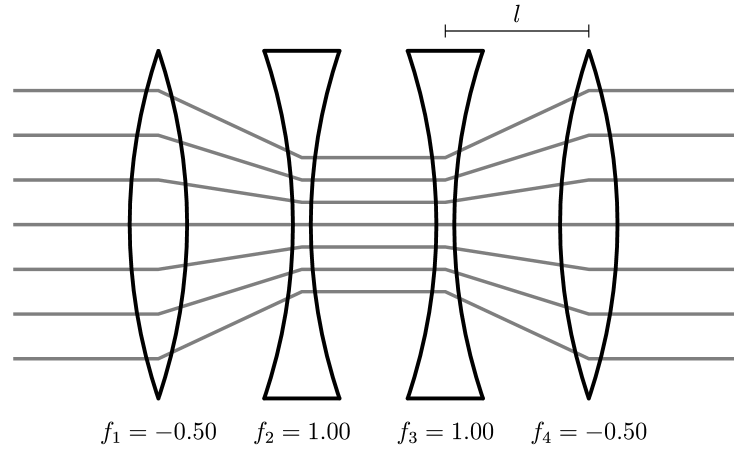
(a) Exemplary initial configuration.

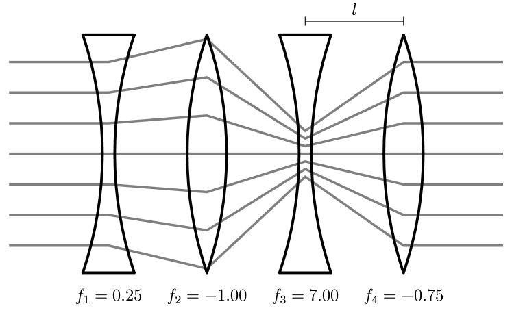
(b) Corrected state. Despite the change of sign of $f_{2}$, the overall optical properties are identical to the initial state.

Figure 2: Schematic representation of the four-lens system in different configurations.

Symbolic transfer matrices of real-world lattices typically consist of long analytical expressions, which renders obtaining solutions to (9) very challenging. To promote better understanding of the proposed method we shall nevertheless provide the reader with an algebraic, worked out example of application. For this purpose, we will apply our method to a beamline consisting of four quadrupole magnets, each separated by a distance $l$. To simplify the calculations in this example, we restrict the problem to preserving the optical properties in just one plane of motion and treat the quadrupole magnets as thin lenses. The symbolic $2\times 2$ transfer matrix $\mathcal{M}$ in this plane of motion is given by

$$\mathcal{M}=\mathcal{L}(f_{4})\cdot\mathcal{D}(l)\cdot\mathcal{L}(f_{3})\cdot\mathcal{D}(l)\cdot\mathcal{L}(f_{2})\cdot\mathcal{D}(l)\cdot\mathcal{L}(f_{1}),$$

where $\mathcal{L}(f)$ is the known transport matrix of a thin lens with focal strength $f$, while $\mathcal{D}(l)$ represents a drift space,

$$\mathcal{L}(f)=\begin{pmatrix}1&0\\ f&1\end{pmatrix}\qquad\mathcal{D}(l)=\begin{pmatrix}1&l\\ 0&1\end{pmatrix}.$$

Suppose the system is in an arbitrary initial configuration $f_{i}=f_{i}^{*}$, as for example depicted in Figure 2(a). If now the focal strength of one lens is altered, the resulting optics will deviate from the initial case. The goal of this example is to calculate functions for the focal strengths $f_{1}$, $f_{3}$ and $f_{4}$ that correct any influence variation of $f_{2}$ has on the transfer matrix of the system.

According to equation (1), $\mathcal{M}$ has three independent elements. Therefore, we can choose three arbitrary elements of $\mathcal{M}$ for the definition of $\bm{B}$. We might choose

$$\bm{B}=(\mathcal{M}_{11},\mathcal{M}_{12},\mathcal{M}_{22})^{T}=$$

$$\scalebox{0.95}{$\left(\begin{array}[]{c}l\left(f_{2}\left(f_{3}l+2\right)+f_{1}\left(2f_{3}l+f_{2}l\left(f_{3}l+2\right)+3\right)+f_{3}\right)+1\\ l\left(2f_{3}l+f_{2}l\left(f_{3}l+2\right)+3\right)\\ 3f_{4}l+2f_{3}l\left(f_{4}l+1\right)+f_{2}l\left(f_{3}l+f_{4}l\left(f_{3}l+2\right)+1\right)+1\\ \end{array}\right)$}.$$

We define the correction parameters to be the focal strengths of the remaining lenses

$$\tau=(f_{1},f_{3},f_{4})^{T}.$$

In this case, equation (9) yields the following differential equations

$$\begin{pmatrix}\dfrac{\textrm{d}f_{1}}{\textrm{d}f_{2}}\\ \dfrac{\textrm{d}f_{3}}{\textrm{d}f_{2}}\\ \dfrac{\textrm{d}f_{4}}{\textrm{d}f_{2}}\end{pmatrix}=\left(\begin{array}[]{c}-\dfrac{f_{3}l+2}{\left(f_{2}l+2\right)\left(2f_{3}l+f_{2}l\left(f_{3}l+2\right)+3\right)}\\ -\dfrac{f_{3}l+2}{f_{2}l+2}\\ \dfrac{1}{2f_{3}l+f_{2}l\left(f_{3}l+2\right)+3}\\ \end{array}\right).$$

The solution to these equations for the initial conditions $f_{i}(f_{2}^{*})=f_{i}^{*}$ are

$$f_{1} =\dfrac{f^{*}_{1}\left(f_{2}l+2\right)\left(2f^{*}_{3}l+f^{*}_{2}l\left(f^{*}_{3}l+2\right)+3\right)-\left(f_{2}-f^{*}_{2}\right)\left(f^{*}_{3}l+2\right)}{\left(f_{2}l+2\right)\left(2f^{*}_{3}l+f^{*}_{2}l\left(f^{*}_{3}l+2\right)+3\right)}$$

$$f_{3} =\dfrac{f^{*}_{2}\left(f^{*}_{3}l+2\right)+2f^{*}_{3}-2f_{2}}{f_{2}l+2}$$

$$f_{4} =\dfrac{f_{2}-f^{*}_{2}}{2f^{*}_{3}l+f^{*}_{2}l\left(f^{*}_{3}l+2\right)+3}+f^{*}_{4}.$$

For every value of $f_{2}$ these functions yield values for the remaing focal strengths, so that the optical properties of the system are equivalent to those of the initial setting $f_{i}^{*}$, see for example Figure 2(b). It can be seen that the first two functions have a pole at $f_{2}=-2/l$, independent on the initial condition. At this point the Jacobian determinant in equation (6) vanishes and no continuous correction beyond this point is possible.

IV Implementation at sFLASH

Figure 3: Positions of the quadrupole magnets close to the SFLASH undulator. Note that the magnets in the SFUND section can not be used as correctors. Magnets used in the example shown in Figure 4 are highlighted in red. Drawing not to scale.

The super-conducting linear accelerator FLASH at DESY in Hamburg delivers trains of electron bunches into two parallel undulator beamlines, FLASH1 and FLASH2. While FLASH2 is currently being prepared for user operation, FLASH1 has been delivering soft x-ray photons for user experiments since 2005 Honkavaara et al. (2014). Upstream of the FLASH1 main undulator an experimental setup for FEL seeding (sFLASH) is located, see Figure 1. It features four variable-gap undulator modules and thus is the ideal test bench for the study of several different seeding schemes Bödewadt et al. (2015).

Closing the seeding undulator intensifies its natural focusing effect and will therefore impact the beam optics further downstream of this undulator and in particular at the entrance of the main undulator. At lower beam energies the change in the $\beta$-function can easily be in the order of several tens of percent so that the matching into the FODO structure of the main undulator is corrupted. The result is a significantly deteriorated FEL performance. Therefore, the disturbance introduced by the seeding undulator has to be compensated by adjusting the field strength of appropriate quadrupole magnets.

Initially, the presented method was developed to correct for the influence of the variable-gap undulator used by the seeding experiment at FLASH. Due to their magnetic structure, planar undulators exhibit a systematic focusing effect in the vertical plane (here, denoted by $y$), perpendicular to their pole faces. For our purpose, the additional weak defocusing in the horizontal direction ($x$), stemming from the finite width of real-world undulators, can be neglected. Employing the matrix formalism introduced above, the effect of an undulator of length $l$ and undulator period $\lambda_{\mathrm{u}}$ on a particle’s trajectory vector $u=\left(x,x^{\prime},y,y^{\prime}\right)^{T}$ is represented by the transfer matrix

$$\mathcal{M}_{\mathrm{und}}=\begin{pmatrix}1&l&0&0\\ 0&1&0&0\\ 0&0&\mathrm{cos}\sqrt{\kappa}l&\frac{\mathrm{sin}\sqrt{\kappa}l}{\sqrt{\kappa}}\\ 0&0&-\sqrt{\kappa}\,\mathrm{sin}\sqrt{\kappa}l&\mathrm{cos}\sqrt{\kappa}l\end{pmatrix},$$ (10)

where $\kappa$ is the focusing strength

$$\kappa\approx 2\left(\dfrac{K\,\pi}{\gamma\lambda_{\mathrm{u}}}\right)^{2},$$ (11)

defined by the undulator parameter $K$ and $\gamma$, the particle’s Lorentz factor Quattromini et al. (2012). By varying the value of the gap, the $K$ parameter of the undulator system used by the sFLASH experiment can be set to a value between $0$ and $2.72$ Tischer et al. (2010), introducing the undesirable focusing effect. We therefore identify $K$ as the disturbance parameter.

Our implementation utilizes the computer algebra system Mathematica Wolfram Research, Inc. (2014), which allows for easily calculating the required symbolic transfer matrix according to equation (2), as well as setting up the differential equations (9), the numerical solution of which is then found by means of a basic Runge-Kutta algorithm. There are $14$ quadrupole magnets in the vicinity of the sFLASH undulator (see Figure 3) that are included in the Mathematica model and are available as correctors. As our method produces correction functions for exactly $6$ parameters there are

$$\binom{14}{6}=3003$$

combinations of corrector magnets to choose from. Investigation shows that a lot of these combinations are prone to produce solutions featuring impracticably high changes in the quadrupole strengths or solutions containing a singularity, as mentioned above. However, we were able to identify a set of known good corrector combinations for optics similar to the standard optics used in nominal SASE operation. An example of the correction functions that are obtained by this method is shown in Figure 4.

Surely, for any given manipulation, correction functions exist which involve more than six corrector magnets. In that case, the solution of equation (5) is no longer unique because, as we have seen, solutions can be constructed using any combination of six of the magnets and leave the others constant, which results in our method being not directly applicable. However, any number of additional constraints, other than those given by the constancy of the transfer matrix, can easily be incorporated into our method by appending them to $\bm{B}$ in equation (5) and selecting the same number of additional correction parameters.

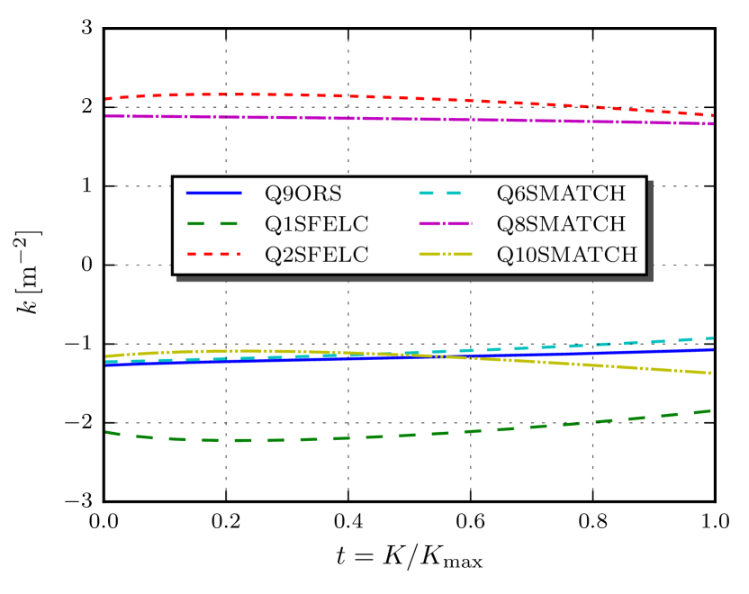
Figure 4: Example of a correction function calculated using the presented method. Here, the strengths $k$ of the six named quadrupole magnets are used as correction parameters to compensate for the optics disturbance caused by the sFLASH undulator being closed from $K=0$ to $K=K_{\textrm{max}}=2.63$ at a beam energy of $693\text{\,}\mathrm{MeV}$.

While our method assures the constancy of the transfer matrix between the first and the last corrector magnet, it however makes no statement about the behavior of the optical functions within this correction section. Using the particle tracking code ELEGANT, the optics can be checked for unwanted features and the efficacy of the correction can be verified, see Figure 5.

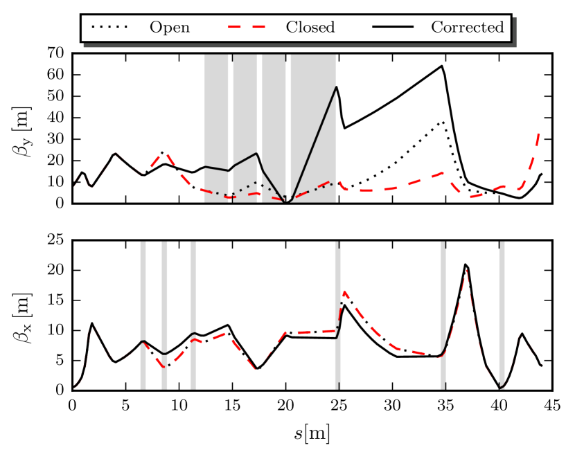
Figure 5: Development of the $\beta$-functions in dependence on the longitudinal coordinate $s$. The undisturbed state (dotted) is compared to the disturbed state with (solid line) and without (dashed) application of the correction. Grey areas in the upper plot mark the position of the variable-gap undulator segments. In this example, a different set of correction magnets is used. Their positions are indicated in the lower plot. Note that at the end of the beamline the corrected optical functions agree with the open case.

V Measurements

Diagnostics in the FLASH1 main undulator area include wire scanners at the ends of the undulator modules. With the help of these devices the beam diameter can be determined along the undulator. The relationship between beam size $\sigma$ and $\beta$-function in the vertical and horizontal direction is given by the well known equation

$$\sigma_{u}(z)=\sqrt{\varepsilon_{u}\,\beta_{u}(z)},\quad u\in\{x,y\},$$ (12)

where $z$ is the longitudinal position and $\varepsilon_{u}$ denotes the beam emittance. A successful correction can therefore be verified experimentally, by comparing the beam sizes along the undulator.

The measurements presented in Figure 6 have been conducted with a 1.0-GeV-electron beam, while the disturbance was introduced by closing all four seeding undulator segments to their lowest gap value.

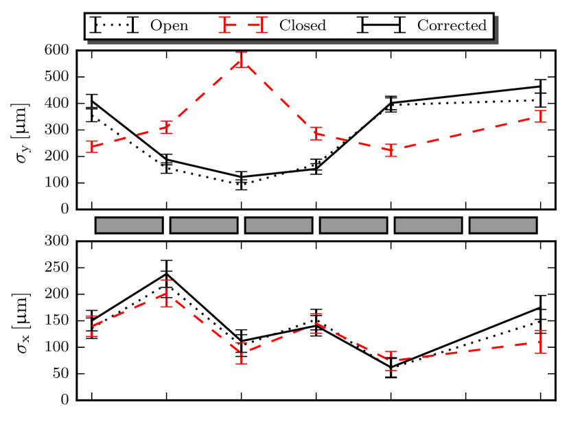
Figure 6: Transverse beam sizes measured using the wire scanners between the six FLASH main undulator segments (grey boxes in the middle). The dotted curve shows the beam sizes at theory optics without any disturbance. Measurements of the disturbed case, where the seeding undulator is closed, are depicted by the dashed curve. The solid curve shows beam sizes with corrections applied. At the time of measurement, the wire scanner between the last two undulator segments was unavailable [Figures\ref{fig:correction}; \ref{fig:betaplot}and\ref{fig:wirescans}werecreatedusingmatplotlib.]Hunter2007.

As expected, closing the seeding undulator primarily affects the beam size in the vertical direction. After the optics correction is applied, the beam sizes correspond to those measured with an open undulator within the range of measuring accuracy. Thereby, it is shown experimentally that our method is able to restore the initial course of the optical functions in the main undulator with satisfactory precision.

As mentioned above, the motivation leading to the development of the presented method was to allow simultaneous operation of both the sFLASH and FLASH1 main undulator. In recent efforts to establish procedures for three beamline lasing (FLASH1, FLASH2, sFLASH) the described method is in frequent use Plath et al. (2016). Once FLASH1 SASE operation is established, the sFLASH variable-gap undulator segments are closed to their target gap values, causing the SASE signal of the main undulator to vanish. Subsequently, the calculated correction is applied to the chosen corrector quadrupole magnets. This on-line procedure was able to recover 70% of the initial FEL photon pulse energy with only a few orbit corrections applied.

VI Conclusion and Outlook

We developed a novel approach to compensate for variations in particle beam optics that would otherwise disturb the optics in other parts of the machine, if let uncorrected. It produces continuous, numerical functions for six machine parameters, compensating the unwanted effect of an arbitrary number of disturbance parameters. Because of the continuity of the correction function, it is suitable to be applied simultaneously to the disturbance. Effectively, this method allows to freely modify the optics locally within a beamline section, without altering the optics in the rest of the machine.

The method has been implemented at FLASH, with the objective of compensating the influence of the variable-gap undulator used by the sFLASH experiment and is in frequent use. We showed measurements confirming the precise restoration of the initial optics.

A next experimental step will be to apply the correction steadily as the disturbance arises, which in the end enables us to close the seeding undulator and start seeding experiments without any notable changes of electron beam quality in the FLASH1 main undulator. This compensation constitutes an important milestone for the planned simultaneous operation of a seeding experiment at FLASH1. The method will generally be useful for two FELs operated independently of each other in cascaded mode. Ultimately, it will be beneficial for all optics manipulations that need to stay restricted to a local section of a long beamline.