Superradiance induced particle flow via dynamical gauge coupling

Abstract

We study fermions that are gauge-coupled to a cavity mode via Raman-assisted hopping in a one dimensional lattice. For an infinite lattice, we find a superradiant phase with infinitesimal pumping threshold which induces a directed particle flow. We explore the fate of this flow in a finite lattice with boundaries, studying the non-equilibrium dynamics including fluctuation effects. The short time dynamics is dominated by superradiance, while the long time behaviour is governed by cavity fluctuations. We show that the steady state in the finite lattice is not unique, and can be understood in terms of coherent bosonic excitations above a Fermi surface in real space.

Quantum matter interacting with gauge fields is a central topic of modern physics. In cold atom systems, although atoms are charge neutral, Abelian or non-Abelian synthetic gauge potentials can be simulated by various methods2011revGF 2013revGF , such as rotation2009rotation , magnetic gradients2014monopole , two-photon Raman transitions2009vectorpotential 2009magneticfield 2011SOC , laser-assisted hoppingBloch2011 Bloch2013 MIT2013 Bloch2015 , and lattice “shaking”2011Shakinglattice . However, simulation of a dynamical gauge field, possessing its own quantum dynamics, is still a great challenge2012DynamicGF 2013DynamicGF .

On the other hand, subjecting quantum gases to optical cavitiesrev2013 has drawn a lot of attention in recent years. The coupling between cold atoms and the quantized cavity modes can dramatically change the properties of both the atomic gas and the cavity field. For example, a Bose-Einstein condensate coupled to a cavity can undergo a quantum phase transition to a supersolid phase. At the same time, the cavity field enters the “superradiant” phase with a non-zero expectation valueEsslinger2010 Esslinger2012 Esslinger2015v2 Ritsch2002 Domokos2010 . The Bose-Hubbard model inside a cavity exhibits a rich phase diagram, due to cavity-induced long range interactions between atomsHemmerich2015r2 Hemmerich2015 Esslinger2015 . These successful experiments have stimulated many theoretical studies in this direction2009Simons 2010Goldbart 2013Diehl Simons2014 Piazza2014 Zhai2014 Yi2014 Pu2014 Yu2015 Yi2015 2015hopping 2016Kollath Zhai2015 2016hopping 2016Donner . Dissipation of the cavity field, through photon loss, causes significant back action on the atomic system, on both its dynamicsKonya2014 and its steady state distributionGriesser2010 Griesser2011 Schutz2013 Piazzal2014 .

In this letter, we study the steady states and the non-equilibrium dynamics of fermions in a one dimensional cavity-assisted hopping lattice. The phase of the cavity mode acts on the atoms as a vector potential, which has its own quantum dynamics controlled by the atom distribution. This system differs from the models in Refs.2016Kollath 2016hopping , where the cavity-assisted hopping acts only between two legs of a ladder. Allowing hopping along an infinite lattice, we find a transition, at infinitesimal pumping threshold, to a superradiant phase in which the gauge coupling induces a directed persistent current. In a finite lattice, with open boundary conditions, we show that there can be no superradiant steady state. We study the non-equilibrium dynamics in the finite lattice, incorporating fluctuation effects beyond mean field. On short time scales, particles flow by coherent hopping as for the infinite lattice, while in the long time limit, dissipation dominates particle transport and determines the steady state. Through a mapping to collective bosonic modes in real space, we show that this steady state is not unique.

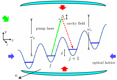
Figure 1: The setup for cavity-assisted hopping on a lattice. A large energy offset $\delta$ prevents direct tunneling between neighbouring sites. The atoms can hop by a cavity-assisted Raman process, absorbing a pump photon at $\omega_{p}$ (solid green arrow) and emitting a photon at $\omega_{p}-\delta$ into the cavity (red dashed arrow). This emission is detuned from the cavity mode, $\omega_{c}$, by $\Delta\ll\delta$. Cavity losses are described by $\kappa$.

Model.– We consider spinless atoms trapped by an optical lattice in a high-Q cavity, Fig.1. The optical lattice is in the $x$-direction, while the cavity mode is in the $y$-direction. The atom cloud is illuminated by a pump laser in the $z$-direction. We consider a strong transverse confinement to prohibit momentum transfer to the atoms, so the system is quasi one dimensional. By accelerating the optical lattice or applying a gradient magnetic field, an energy gradient can be imposed along the $x$-direction so that direct hopping is suppressed by a large energy offset $\delta$ between lattice sites. An atom can hop to the right by a Raman process, absorbing a pump photon ($\omega_{p}$) and emitting at $\omega_{p}-\delta$. (We assume $\omega_{p}$ to be far detuned from the optical transition so the excited state population can be neglected.) We consider this emission to be enhanced by a cavity mode tuned close to this frequency, $\omega_{c}\simeq\omega_{p}-\delta$. (We assume that $\delta$ is sufficiently large that emission at $\omega_{p}+\delta$, corresponding to a hop to the left, is negligible.) We make a tight-binding approximation to obtain the effective Hamiltonian ($\hbar=1$ throughout):

$$\hat{H}=\Delta\hat{a}^{{\dagger}}\hat{a}-\sum_{j=1}^{L-1}\left(\lambda\hat{a}^{{\dagger}}\hat{c}_{j+1}^{{\dagger}}\hat{c}_{j}+\lambda^{\ast}\hat{a}\hat{c}_{j}^{{\dagger}}\hat{c}_{j+1}\right)\,.$$ (1)

Here $\hat{a}$ is the field operator of the cavity photon expressed in a frame rotating at the frequency $\omega_{p}-\delta$ for which intersite hopping is resonant; $\Delta\equiv\delta-\omega_{p}+\omega_{c}$ is the detuning of the cavity mode from resonance; and $\hat{c}_{j}^{({\dagger})}$ are fermionic field operators on lattice sites $j$. (We shall also mention some results for hard-core bosons.) The cavity-assisted hopping $\lambda\hat{a}^{{\dagger}}$ has a phase given by the phase difference between the cavity field and the pump laser. We choose to set the phase of the pump to zero, $\lambda^{\ast}=\lambda$, such that the hopping phase equals the phase of the cavity field.

If the cavity were replaced by a second drive laser, at frequency $\omega_{p}-\delta$, such that the cavity field operator is replaced by the coherent state $\langle\hat{a}\rangle=\alpha=|\alpha|e^{i\theta}$, then the particles would experience the static Hamiltonian $\hat{H}(\alpha)=-\lambda\sum_{j}\left(\alpha^{\ast}\hat{c}_{j+1}^{{\dagger}}\hat{c}_{j}+\alpha\hat{c}_{j}^{{\dagger}}\hat{c}_{j+1}\right)$. The corresponding dispersion relation (for an infinite lattice) is

$$E_{k}=-2\lambda\left|\alpha\right|\cos\left(k+\theta\right)$$ (2)

for a particle of momentum $k$. Thus, the phase of the cavity field, $\theta$, couples to the particles as a vector potential. In this driven case, the vector potential is static, set by the phase difference between the two driving lasers. Henceforth we shall treat the cavity field as dynamical, so the vector potential inherits its own quantum dynamics, linked to the distribution of particles. This differs from the cavity-assisted hopping in Refs.2015hopping 2016Kollath , where the hopping phase is fixed, and only the amplitude is dynamical.

Superradiance.– The leakage of photons from the cavity requires the full dynamics to be described by the Lindblad master equation, $\partial_{t}\rho=-i\left[\hat{H},\rho\right]+\mathcal{L}[\rho]$, where $\rho$ is the density matrix, and the Lindblad superoperator reads $\mathcal{L}[\rho]=\kappa\left(2\hat{a}\rho\hat{a}^{{\dagger}}-\hat{a}^{{\dagger}}\hat{a}\rho-\rho\hat{a}^{{\dagger}}\hat{a}\right)$. This describes a cavity photon loss rate of $2\kappa$. The mean cavity field, $\left\langle\hat{a}(t)\right\rangle=\alpha(t)$, evolves as:

$$\partial_{t}\alpha=-i\left(\Delta-i\kappa\right)\alpha+i\lambda K,$$ (3)

where $K\equiv\langle\hat{K}\rangle$, with $\hat{K}\equiv\sum_{j=1}^{L-1}\hat{c}_{j+1}^{{\dagger}}\hat{c}_{j}$ the operator that couples to the cavity field (1). For steady states, $\partial_{t}\alpha=0$, we obtain

$$\alpha=\frac{\lambda K}{\Delta-i\kappa}.$$ (4)

with $\Delta$, $\kappa$ and $\lambda$ real parameters.

Consider first an infinitely long lattice. In this case, one can write $K=\sum_{k}e^{-ik}\left\langle\hat{n}_{k}\right\rangle$, where $\hat{n}_{k}$ counts the number of particles of momentum $k$. These occupations are conserved, $[\hat{n}_{k},\hat{H}]=0$, so $\lambda K$ in Eq. (3) can be treated as an external source, determined by the initial momentum distribution. Provided the initial distribution has $|K|\neq 0$, the steady state has $|\alpha|\neq 0$, i.e. there is no threshold for superradiance. This differs from the usual Dicke-type setupDicke1954 , where superradiance appears only above a critical pumping strength.

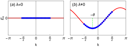
Figure 2: Mean field band structure and momentum distribution of fermions. (a) No pumping field, $\lambda=0$. (b) Non-zero pumping strengh, $\lambda\neq 0$. Here $k=-\theta$ is the minimum of the band.

Although the cavity field cannot change the momentum distribution of the atoms, the emergence of superradiance dramatically alters their dispersion (2). We find that superradiance leads to a directed persistent current. From (2) the particle velocity is $v_{k}=2\lambda\left|\alpha\right|\sin\left(k+\theta\right)$, so the total current, $J=\sum_{k}v_{k}\left\langle\hat{n}_{k}\right\rangle$, may be written $J=-2\lambda\mathrm{Im}\left(\alpha^{\ast}K\right)$. Thus, there will be a non-zero net current if the phases of $K$ and $\alpha$ differ. From Eq.(4), such a phase difference appears whenever there is cavity loss, $\kappa\neq 0$. For example, consider a half-filled system with $\left\langle\hat{n}_{k}\right\rangle=\Theta\left(\left|k\right|-\pi/2\right)$, see Fig. 2(a). One finds a real $K=L/\pi$, while the phase is $\tan\theta=\kappa/\Delta$. The minimum of the band is shifted to $k=-\theta$, such that the momentum distribution is unsymmetrical about it, see Fig. 2(b). This leads to an imbalance of left and right moving particles, resulting in a net current to the right. Thus, the dynamical vector potential self-organizes to induce a particle current. Indeed, on resonance, $\Delta=0$, the steady state value of cavity phase $\theta$ maximizes the current ($\frac{\partial J}{\partial\theta}=0$).

The importance of dissipation for the net current can also be seen by substituting Eq. (4) into the expression for the total current, giving $J=2\kappa\left|\alpha\right|^{2}$. This has a simple interpretation. For a cavity occupation of $|\alpha|^{2}$ the rate of photon loss is $2\kappa\left|\alpha\right|^{2}$. To maintain the population $|\alpha|^{2}$, the scattering of pump photons into the cavity should compensate this loss. Each atom that scatters a photon from pump to cavity undergoes a hop by one site to the right, thus leading to a net current of $2\kappa\left|\alpha\right|^{2}$.

Now we switch to the finite lattice with open boundary conditions. The boundaries break translational invariance: momentum is no longer conserved, so the cavity field can have a feedback on the distribution of the atoms. At mean field level, the equation-of-motion of the fermionic density matrix, $\rho_{ij}(t)=\left\langle\hat{c}_{i}^{{\dagger}}(t)\hat{c}_{j}(t)\right\rangle$, is

$$\partial_{t}\rho_{ij}(t)=-i\lambda A_{ij}(t),$$ (5)

where $A_{ij}=\alpha^{\ast}\rho_{i+1,j}+\alpha\rho_{i-1,j}-\alpha^{\ast}\rho_{i,j-1}-\alpha\rho_{i,j+1}$. Imposing the boundary conditions $A_{1,1}=\alpha^{\ast}\rho_{2,1}-\alpha\rho_{1,2}$ and $A_{L,L}=\alpha\rho_{L-1,L}-\alpha^{\ast}\rho_{L,L-1}$, we can prove $\alpha^{\ast}K=\alpha K^{\ast}$ in any steady statesup . Combining with Eq.(4), we find that the only steady state solution is $\alpha=K=0$. The essential physics is that the boundaries preclude the steady state from carrying a net current, so the net photon scattering rate from pump mode to cavity mode must vanish. Independent of initial state, the mean-field steady state is one with $K=0$ and no superradiance, $\alpha=0$.

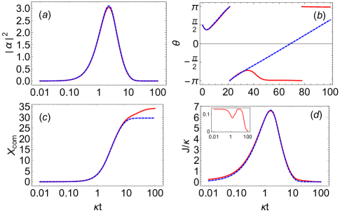
Figure 3: The non-equilibrium dynamics of the cavity mode and the fermions. (a) The cavity field occupation $\left|\alpha(t)\right|^{2}$; (b) the phase of $\alpha(t)$; (c) the centre-of-mass of the fermions; (d) the total current of the fermions. Inset shows the current beyond mean field, $J^{\mathrm{cl}}+J^{\mathrm{qu}}$. The blue dashed lines are the mean field results with lattice length $L=20$, particle number $N=5$, detuning $\Delta/\kappa=0.5$, and $\lambda/\kappa=0.5$. The red solid lines are the results beyond mean field by solving Eq.(6) with the same parameters.

Non-equilibrium dynamics.– If the particles start from a state with non-zero $|K|$, then, even in a finite lattice, the dynamics will first build up the cavity population $\left|\alpha\right|^{2}\neq 0$. However, any eventual steady state must have $\alpha=K=0$. To understand how the particles redistribute themselves in a finite lattice, we study the non-equilibrium dynamics. Combining Eq.(3) and Eq.(5) describes the coupled mean field dynamics of cavity field and fermions. However, one can see from Eq.(5) that for $\alpha\rightarrow 0$ the fermions cannot hop. This is incorrect, since fluctuations of the cavity field will cause fermions to hop. To describe these fluctuation effects in the dynamics, we employ the Keldysh formulation of open quantum systemsDiehl2015 book1 , and use the quasi-particle approximation to obtain the equation-of-motion of the single-particle density matrix assup :

$$\partial_{t}\rho_{ij}=-i\lambda A_{ij}(t)+\frac{\kappa\lambda^{2}}{\Delta^{2}+\kappa^{2}}B_{ij}(t),$$ (6)

which supplements (5) with fluctuation corrections, $B_{ij}(t)=2\rho_{i-1,j-1}-2\rho_{i,j}-\sum_{l}\left(\rho_{i-1,l-1}\rho_{l,j}+\rho_{i,l}\rho_{l-1,j-1}\right)+\sum_{l}\left(\rho_{i+1,l+1}\rho_{l,j}+\rho_{i,l}\rho_{l+1,j+1}\right)$. Here we ignore terms of higher order than $\lambda^{2}$, e.g. cavity-induced interactions between particles at order $\lambda^{4}$, which is valid for $\lambda\ll\kappa$. From the diagonal elements, i.e. the particle density $\rho_{i}=\rho_{ii}$, and the continuity equation, $\partial_{t}\rho_{i}+J_{i}-J_{i-1}=0$, we derive the current $J_{i}$. We find that the current can be separated into three parts, $J_{i}=J_{i}^{\mathrm{sr}}+J_{i}^{\mathrm{cl}}+J_{i}^{\mathrm{qu}}$, where $J_{i}^{\mathrm{sr}}=-\lambda\mathrm{Im}\left(\alpha^{\ast}\rho_{i+1,i}\right)$, is the superradiant current as in mean field. The current $J_{i}^{\mathrm{cl}}=\frac{2\kappa\lambda^{2}}{\Delta^{2}+\kappa^{2}}\left(1-\rho_{i+1}\right)\rho_{i}$ describes the semiclassical current, subject to Pauli blocking, arising from dissipative losses of the fluctuating cavity mode. This current is precisely that for classical driven-dissipative models such as the asymmetric exclusion process (ASEP)ASEP2006 ASEP2007 , which has interesting dynamical phase transitions sensitive to boundary conditions. The contribution $J_{i}^{\mathrm{qu}}=-\frac{2\kappa\lambda^{2}}{\Delta^{2}+\kappa^{2}}\sum_{l\neq i}\mathrm{Re}\left(\rho_{i+1,l+1}\rho_{l,i}\right)$, is a quantum correction to the semiclassical current induced by correlations and involving long-range coherence imposed by the fact that the cavity mode couples to all atoms. Here we see that even when the superradiance vanishes, $\alpha=0$, the fluctuations of the cavity mode can induce a nonzero current $J_{i}^{\mathrm{cl}}+J_{i}^{\mathrm{qu}}$.

We have solved Eq.(6) combined with Eq.(3) numerically. Representative results are plotted in Fig.3. We choose the initial state to be the groundstate of $N$ free fermions in a finite lattice with non-zero hopping, and the cavity mode empty. Because this initial particle state has coherence in real space, $K$ is non-zero and, according to Eq.(3), it will first generate a superradiant state. Indeed, we find that the cavity occupation $|\alpha(t)|^{2}$ grows from zero, and reaches its maximum during a time interval $\tau_{1}\sim\kappa^{-1}$ Fig.3(a). After that, due to the cavity loss, the superradiance decays to zero on a time scale $\tau_{2}\sim\frac{\kappa\pi^{2}\nu\left(1-\nu\right)}{2\lambda^{2}\sin^{2}\left(\pi\nu\right)}$, where $\nu$ is the particle filling. This superradiant pulse is similar to those observed by illuminating degenerate quantum gases in free space1999Ketterle 2011Zhang . Thus, the dynamics can be separated into two regimes. At short times $t\lesssim\tau_{1}+\tau_{2}$, the particle dynamics is dominated by coherent hopping, which is assisted by the mean field part of the cavity field. In this regime, the centre-of-mass of the fermions, $X_{\mathrm{com}}=\sum_{j}j\left\langle\hat{c}_{j}^{{\dagger}}\hat{c}_{j}\right\rangle$, increases quickly, see Fig.3(c). At long times, $t\gg\tau_{1}+\tau_{2}$, the superradiance dies, and the particle dynamics is governed by the dissipative hopping. See Fig.3(c), after the collapse of superradiance, the mean field solution of $X_{\mathrm{com}}(t)$ saturates, while the solution including fluctuations shows that $X_{\mathrm{com}}(t)$ still grows slowly, until finally reaching a slightly larger final steady-state value.

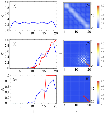
Figure 4: (a) The density distribution of initial state. (b) The absolute value of single-particle density matrix of initial state, $\left|\rho_{ij}(0)\right|$. (c)(d) The final density distribution and density matrix of fermions (beyond mean field) after a long time evolution $\kappa t=1000$. (e)(f) The final density distribution and density matrix of hard core boson starting from same initial state. Blue dashed lines are the mean field results, while the red solid lines are the solutions beyond mean field. The lattice length $L=20$, particle number $N=5$, detuning $\Delta/\kappa=0.5$, and $\lambda/\kappa=0.5$.

To explore the final steady states that are reached long after superradiance has vanished (so $J^{\mathrm{sr}}=0$), in Fig.4(c,d) we plot the density distribution and the density matrix for the fermions at very late times, $\kappa t=1000$. Before discussing the results for fermions, it is helpful to consider the final steady state for the case of hard core bosons, see Fig.4(e,f). For hard core bosons, the steady-state density distribution is a simple step function, i.e. the rightmost $N$ sites are fully populated, while others have no population. The single-particle density matrix shows no coherence. Since all the particles are blocked at the right side, no particle can hop to the right due to the hard core repulsion, giving zero semiclassical current, $J^{\mathrm{cl}}=0$. Vanishing coherence indicates the quantum correlation current $J^{\mathrm{qu}}$ is also zero. The situation is different in the case of fermions. As seen in Fig.4(c,d), the density distribution is not a step function, while the density matrix retains non-zero correlations. In this case, the semiclassical current and its quantum correction do not separately vanish, instead, they cancel each other in the steady state, with $J^{\mathrm{cl}}+J^{\mathrm{qu}}=0$. The quantum correction current and semiclassical current counteract each other in the case of fermions, while they add together in the case of bosons.

Steady states.– To understand the steady states, we adiabatically eliminate the cavity fieldRitsch2005 , making use of the fact that superradiance is absent, $\alpha=\langle\hat{a}\rangle=0$. We obtain the master equation for the fermion density matrix, $\partial_{t}\rho_{\mathrm{f}}=-i\left[\hat{H}_{\mathrm{eff}},\rho_{\mathrm{f}}\right]+\frac{\kappa\lambda^{2}}{\Delta^{2}+\kappa^{2}}\left(2\hat{L}_{\mathrm{eff}}\rho_{\mathrm{f}}\hat{L}_{\mathrm{eff}}^{{\dagger}}-\hat{L}_{\mathrm{eff}}^{{\dagger}}\hat{L}_{\mathrm{eff}}\rho_{\mathrm{f}}-\rho_{\mathrm{f}}\hat{L}_{\mathrm{eff}}^{{\dagger}}\hat{L}_{\mathrm{eff}}\right)$, where $\hat{L}_{\mathrm{eff}}=\hat{K}$ is the effective Liouvillian operator, and the effective Hamiltonian reads $\hat{H}_{\mathrm{eff}}=-\frac{\kappa\lambda^{2}}{\Delta^{2}+\kappa^{2}}\hat{K}^{{\dagger}}\hat{K}$. Any pure state $\left|D\right\rangle$ for which $\hat{H}_{\mathrm{eff}}\left|D\right\rangle=E\left|D\right\rangle$ and $\hat{L}_{\mathrm{eff}}\left|D\right\rangle=0$ is a steady stateDiehl2008 Zoller2010 . Here, these two conditions reduce to $\hat{K}\left|D\right\rangle=0$. It can readily be verified that the step function state, $\left|\mbox{step}\right\rangle\equiv\prod_{j=1}^{N}\hat{c}_{L-N+j}^{{\dagger}}\left|0\right\rangle$, in which the $N$ particles occupy the $N$ states furthest to the right, is a steady state. However we can also find other steady states. To construct these we define the bosonic operators

$$\hat{b}_{s}^{{\dagger}}=\sum_{j=s+1}^{L}\hat{c}_{j-s}^{{\dagger}}\hat{c}_{j},$$ (7)

where $s=1,\cdots,L-1$. These are analogous to the bosonic operators used to solve the Tomonaga-Luttinger model, but now with real space separation $s$ replacing momentum and with $|\mbox{step}\rangle$ viewed as a Fermi sea in real space (with states occupied for $j>L-N$ and empty for $j\leq L-N$). One can verify that the state with one particle-hole excitation above this Fermi sea, created by applying one bosonic operator $\hat{b}_{s}^{{\dagger}}\left|\mbox{step}\right\rangle$, is a steady state, via $\hat{K}\hat{b}_{s}^{{\dagger}}\left|\mbox{step}\right\rangle=\left[\hat{K},\hat{b}_{s}^{{\dagger}}\right]\left|\mbox{step}\right\rangle=0$ if $s\neq 1$ and $s\leq\mathrm{Min}\left(L-N,N\right)$. Similarly, for $n_{\mathrm{b}}$ such bosonic excitations the states $\prod_{\alpha=1}^{n_{\mathrm{b}}}\hat{b}_{s_{\alpha}}^{{\dagger}}\left|\mbox{step}\right\rangle$, are steady states provided $s_{\alpha}\neq 1$, and $\sum_{\alpha}s_{\alpha}\leq\mathrm{Min}\left(L-N,N\right)$. Thus, we can construct a large number of steady states. For $N,(L-N)\rightarrow\infty$ (when all relevant states can be described by bosonic modes), any state that does not involve occupation of the $s=1$ boson is a steady state. This arises because the Liouvillian operator $\hat{K}$ equals the bosonic annihilation operator $\hat{b}_{1}$, so dissipation can only damp the $s=1$ collective mode. This differs from models involving coupling to a macroscopic number of dissipation channelsDiehl2008 Zoller2010 , which lead to unique steady states. The large number of steady states for our model means that different initial conditions will lead to different final steady states.

Final remarks.– Our proposal explores one natural route to a synthetic dynamic gauge coupling in cold atom systems, using elements that can be realized in current experimental conditions. The dynamics of the superradiance can be observed by detecting the photons leaving the cavity, while the redistribution of the fermions could be measured by recently developed fermionic in-situ imaging in optical latticesInsitu01 Insitu02 Insitu03 Insitu04 Insitu05 Zwierlein2016 . It is natural to generalize the setup to the two dimensional case, where the dynamic vector potential can be made spatially dependent to realize a dynamic magnetic field.

I Supplemental material

I.1 The fate of superradiance in a finite lattice with open boundary conditions

From the master equation, we obtain the equations-of-motion of all operators as

$$i\partial_{t}\hat{a} = \left(\Delta-i\kappa\right)\hat{a}-\lambda\sum_{j=1}^{L-1}\hat{c}_{j+1}^{{\dagger}}\hat{c}_{j},$$ (8)

$$i\partial_{t}\hat{c}_{j} = -\lambda\hat{a}^{{\dagger}}\hat{c}_{j-1}-\lambda\hat{a}\hat{c}_{j+1},\text{\ }\left(j\neq 1,L\right).$$ (9)

The open boundary conditions are encoded in the equations-of-motion of $\hat{c}_{1}$ and $\hat{c}_{L}$,

$$i\partial_{t}\hat{c}_{1} = -\lambda\hat{a}\hat{c}_{2},$$ (10)

$$i\partial_{t}\hat{c}_{L} = -\lambda\hat{a}^{{\dagger}}\hat{c}_{L-1}.$$ (11)

Using these equations-of-motion, one obtains the evolution of local fermion density as

$$\partial_{t}\left\langle\hat{c}_{j}^{{\dagger}}\hat{c}_{j}\right\rangle = i\lambda\left\langle\hat{a}^{{\dagger}}\right\rangle\left(\left\langle\hat{c}_{j}^{{\dagger}}\hat{c}_{j-1}\right\rangle-\left\langle\hat{c}_{j+1}^{{\dagger}}\hat{c}_{j}\right\rangle\right)+\lambda\left\langle\hat{a}\right\rangle\left(\left\langle\hat{c}_{j}^{{\dagger}}\hat{c}_{j+1}\right\rangle-\left\langle\hat{c}_{j-1}^{{\dagger}}\hat{c}_{j}\right\rangle\right),$$ (12)

$$\partial_{t}\left\langle\hat{c}_{1}^{{\dagger}}\hat{c}_{1}\right\rangle = -i\lambda\left\langle\hat{a}^{{\dagger}}\right\rangle\left\langle\hat{c}_{2}^{{\dagger}}\hat{c}_{1}\right\rangle+i\lambda\left\langle\hat{a}\right\rangle\left\langle\hat{c}_{1}^{{\dagger}}\hat{c}_{2}\right\rangle,$$ (13)

$$\partial_{t}\left\langle\hat{c}_{L}^{{\dagger}}\hat{c}_{L}\right\rangle = i\lambda\left\langle\hat{a}^{{\dagger}}\right\rangle\left(\left\langle\hat{c}_{L}^{{\dagger}}\hat{c}_{L-1}\right\rangle\right)-i\lambda\left\langle\hat{a}\right\rangle\left\langle\hat{c}_{L-1}^{{\dagger}}\hat{c}_{L}\right\rangle.$$ (14)

In the steady state, $\partial_{t}\left\langle\hat{c}_{j}^{{\dagger}}\hat{c}_{j}\right\rangle=0$, then we have

$$\alpha^{\ast}\left(\left\langle\hat{c}_{j+1}^{{\dagger}}\hat{c}_{j}\right\rangle-\left\langle\hat{c}_{j}^{{\dagger}}\hat{c}_{j-1}\right\rangle\right) = \alpha\left(\left\langle\hat{c}_{j}^{{\dagger}}\hat{c}_{j+1}\right\rangle-\left\langle\hat{c}_{j-1}^{{\dagger}}\hat{c}_{j}\right\rangle\right),$$ (15)

$$\alpha^{\ast}\left\langle\hat{c}_{2}^{{\dagger}}\hat{c}_{1}\right\rangle = \alpha\left\langle\hat{c}_{1}^{{\dagger}}\hat{c}_{2}\right\rangle,$$ (16)

$$\alpha^{\ast}\left\langle\hat{c}_{L}^{{\dagger}}\hat{c}_{L-1}\right\rangle = \alpha\left\langle\hat{c}_{L-1}^{{\dagger}}\hat{c}_{L}\right\rangle.$$ (17)

From these equations, it is straightforward to see $\alpha^{\ast}\left\langle\hat{c}_{j+1}^{{\dagger}}\hat{c}_{j}\right\rangle=\alpha\left\langle\hat{c}_{j}^{{\dagger}}\hat{c}_{j+1}\right\rangle$, where $j=1,\cdots,L-1$. That gives

$$\alpha^{\ast}\sum_{j=1}^{L-1}\left\langle\hat{c}_{j+1}^{{\dagger}}\hat{c}_{j}\right\rangle=\alpha\sum_{j=1}^{L-1}\left\langle\hat{c}_{j}^{{\dagger}}\hat{c}_{j+1}\right\rangle.$$ (18)

This is nothing but $\alpha^{\ast}K=\alpha K^{\ast}$. That indicates the phase shift between $\alpha$ and $K$ is either $0$ or $\pi$. So there can be no superradiant steady state in a finite lattice with open boundary conditions.

I.2 Quantum kinetic equation of the single-particle density matrix of the fermions

From the equations-of-motion (8) and (9), we obtain

$$i\partial_{t}\left\langle\hat{a}\right\rangle = \left(\Delta-i\kappa\right)\left\langle\hat{a}\right\rangle-\lambda\sum_{j}\left\langle\hat{c}_{j+1}^{{\dagger}}\hat{c}_{j}\right\rangle,$$ (19)

$$i\partial_{t}\left\langle\hat{c}_{i}^{{\dagger}}\hat{c}_{j}\right\rangle = \lambda\left[\left\langle\hat{a}^{{\dagger}}\hat{c}_{i+1}^{{\dagger}}\hat{c}_{j}\right\rangle+\left\langle\hat{a}\hat{c}_{i-1}^{{\dagger}}\hat{c}_{j}\right\rangle-\left\langle\hat{a}^{{\dagger}}\hat{c}_{i}^{{\dagger}}\hat{c}_{j-1}\right\rangle-\left\langle\hat{a}\hat{c}_{i}^{{\dagger}}\hat{c}_{j+1}\right\rangle\right].$$ (20)

Then we separate the mean field and the fluctuation parts of the cavity field as

$$\hat{a}(t)=\left\langle\hat{a}(t)\right\rangle+\delta\hat{a}(t)=\alpha(t)+\delta\hat{a}(t),$$ (21)

where the fluctuation operator satisfies the usual bosonic commutation relation, $\left[\delta\hat{a},\delta\hat{a}^{{\dagger}}\right]=1$. Then Eq. (19) and (20) can be rewritten into

$$i\partial_{t}\alpha = \left(\Delta-i\kappa\right)\alpha-\lambda\sum_{j}\rho_{j+1,j},$$ (22)

$$i\partial_{t}\rho_{i,j} = \lambda\left(\alpha^{\ast}\rho_{i+1,j}+\alpha\rho_{i-1,j}-\alpha^{\ast}\rho_{i,j-1}-\alpha\rho_{i,j+1}\right)$$ (23)

$$+\lambda\left[\left\langle\delta\hat{a}^{{\dagger}}\hat{c}_{i+1}^{{\dagger}}\hat{c}_{j}\right\rangle+\left\langle\delta\hat{a}\hat{c}_{i-1}^{{\dagger}}\hat{c}_{j}\right\rangle-\left\langle\delta\hat{a}^{{\dagger}}\hat{c}_{i}^{{\dagger}}\hat{c}_{j-1}\right\rangle-\left\langle\delta\hat{a}\hat{c}_{i}^{{\dagger}}\hat{c}_{j+1}\right\rangle\right]$$

where $\rho_{i,j}(t)=\left\langle\hat{c}_{i}^{{\dagger}}(t)\hat{c}_{j}(t)\right\rangle$, is the single-particle density matrix of fermions. Here the mean field part of the cavity field behaves as an time-dependent potential, which acts on the single-particle dynamics of the fermions. However, these equations are not closed. To deal with this problem, we introduce the Keldysh Green’s function of fermions, which is defined as

$$iG_{ij}^{K}\left(t_{2},t_{1}\right)=\left\langle\left[\hat{c}_{i}(t_{2}),\hat{c}_{j}^{{\dagger}}(t_{1})\right]\right\rangle.$$ (24)

The single-particle density matrix can be calculated from this Keldysh Green function by

$$\rho_{ij}(t) = \frac{1}{2}\left[\delta_{ji}-iG_{ji}^{K}\left(t,t\right)\right],$$ (25)

$$= \frac{1}{2}\left[\delta_{ji}-i\int\frac{d\omega}{2\pi}G_{ji}^{K}\left(t,\omega\right)\right],$$

where $G_{ji}^{K}\left(t,\omega\right)$ is the Wigner transformation of $G_{ji}^{K}\left(t_{2},t_{1}\right)$, which is defined as $G_{ji}^{K}\left(t,\omega\right)=\int d\tau e^{i\omega\tau}G_{ji}^{K}\left(t+\tau/2,t-\tau/2\right)$. So once having the quantum kinetic equation of the Keldysh Green’s function, we can immediately obtain the evolution of the single-particle density matrix. The quantum kinetic equation in terms of the Keldysh Green’s function is given by2007Rammer

$$\left[G_{0}^{-1}-\mathrm{Re}\Sigma^{R},G^{K}\right]_{\circ}+\left[\mathrm{Re}G^{R},\Sigma^{K}\right]_{\circ}=\frac{1}{2}i\left\{A,\Sigma^{K}\right\}_{\circ}-\frac{1}{2}i\left\{\Gamma,G^{K}\right\}_{\circ},$$ (26)

where $G_{0}^{-1}$ is the free Green function, $G^{R\left(A\right)}$ is the retarded(advanced) Green’s function, defined by

$$G_{ij}^{R}\left(t_{2},t_{1}\right) = -i\Theta\left(t_{2}-t_{1}\right)\left\langle\left\{\hat{c}_{i}(t_{2}),\hat{c}_{j}^{{\dagger}}(t_{2})\right\}\right\rangle,$$ (27)

$$G_{ij}^{A}\left(t_{2},t_{1}\right) = -i\Theta\left(t_{1}-t_{2}\right)\left\{\hat{c}_{i}(t_{2}),\hat{c}_{j}^{{\dagger}}(t_{2})\right\},$$ (28)

and $\Sigma^{K\left(R,A\right)}$ is the Keldysh(retarded, advanced) self-energy. The spectrum function $A\left(t_{2},t_{1}\right)$ and lifetime function $\Gamma\left(t_{2},t_{1}\right)$ are given by

$$\Gamma\left(t_{2},t_{1}\right) = i\left[\Sigma^{R}\left(t_{2},t_{1}\right)-\Sigma^{A}\left(t_{2},t_{1}\right)\right],$$ (29)

$$A\left(t_{2},t_{1}\right) = i\left[G^{R}\left(t_{2},t_{1}\right)-G^{A}\left(t_{2},t_{1}\right)\right],$$ (30)

The commutator(anti-commutator) is defined as $\left[f_{1},f_{2}\right]_{\circ}=f_{1}\circ f_{2}-f_{2}\circ f_{1}$($\left\{f_{1},f_{2}\right\}_{\circ}=f_{1}\circ f_{2}+f_{2}\circ f_{1}$), where $f_{1}\circ f_{2}$ denotes the time-space convolution of the two-point function. Employing the quasi-particle approximation, i.e. ignoring the self-energy term in the left hand side, we have:

$$\left[G_{0}^{-1},G^{K}\right]_{\circ}=\frac{1}{2}i\left\{A,\Sigma^{K}\right\}_{\circ}-\frac{1}{2}i\left\{\Gamma,G^{K}\right\}_{\circ},$$ (31)

The left hand side represents the drift of quasi-particles, while the right hand side represents the collision integral. Making the Wigner transformation, and using the gradient approximation, we obtain:

$$i\partial_{t}G_{j_{2}j_{1}}^{K}\left(t,\omega\right) = -\sum_{l}\left\{h_{j_{2}l}(t)G_{lj_{1}}^{K}\left(t,\omega\right)-G_{j_{2}l}^{K}\left(t,\omega\right)h_{lj_{1}}(t)\right\}$$ (32)

$$+\frac{1}{2}i\sum_{l}\left[A_{j_{2}l}(t,\omega)\Sigma_{lj_{1}}^{K}\left(t,\omega\right)+\Sigma_{j_{2}l}^{K}\left(t,\omega\right)A_{lj_{1}}(t,\omega)\right]$$

$$-\frac{1}{2}i\sum_{l}\left[\Gamma_{j_{2}l}(t,\omega)G_{lj_{1}}^{K}\left(t,\omega\right)+G_{j_{2}l}^{K}\left(t,\omega\right)\Gamma_{lj_{1}}(t,\omega)\right].$$

To go further, we have to calculate the Keldysh self-energy $\Sigma_{ij}^{K}\left(t,\omega\right)$ and lifetime function $\Gamma_{ij}(t,\omega)$. By ignoring the correction of the vertex function, we can express the self-energy of fermions as2010Altland

$$\Sigma_{j_{2}j_{1}}^{R}\left(t_{2},t_{1}\right) = i\frac{1}{2}\lambda^{2}\left[D^{K}\left(t_{2},t_{1}\right)G_{j_{2}+1,j_{1}+1}^{R}\left(t_{2},t_{1}\right)+D^{K}\left(t_{1},t_{2}\right)G_{j_{2}-1,j_{1}-1}^{R}\left(t_{2},t_{1}\right)\right]$$ (33)

$$+i\frac{1}{2}\lambda^{2}\left[D^{R}\left(t_{2},t_{1}\right)G_{j_{2}+1,j_{1}+1}^{K}\left(t_{2},t_{1}\right)+D^{A}\left(t_{1},t_{2}\right)G_{j_{2}-1,j_{1}-1}^{K}\left(t_{2},t_{1}\right)\right],$$

$$\Sigma_{j_{2}j_{1}}^{A}\left(t_{2},t_{1}\right) = i\frac{1}{2}\lambda^{2}\left[D^{K}\left(t_{2},t_{1}\right)G_{j_{2}+1,j_{1}+1}^{A}\left(t_{2},t_{1}\right)+D^{K}\left(t_{1},t_{2}\right)G_{j_{2}-1,j_{1}-1}^{A}\left(t_{2},t_{1}\right)\right]$$ (34)

$$+i\frac{1}{2}\lambda^{2}\left[D^{A}\left(t_{2},t_{1}\right)G_{j_{2}+1,j_{1}+1}^{K}\left(t_{2},t_{1}\right)+D^{R}\left(t_{1},t_{2}\right)G_{j_{2}-1,j_{1}-1}^{K}\left(t_{2},t_{1}\right)\right],$$

$$\Sigma_{j_{2}j_{1}}^{K}\left(t_{2},t_{1}\right) = i\frac{1}{2}\lambda^{2}\left[D^{K}\left(t_{2},t_{1}\right)G_{j_{2}+1,j_{1}+1}^{K}\left(t_{2},t_{1}\right)+D^{K}\left(t_{1},t_{2}\right)G_{j_{2}-1,j_{1}-1}^{K}\left(t_{2},t_{1}\right)\right]$$ (35)

$$+i\frac{1}{2}\lambda^{2}\left[D^{R}\left(t_{2},t_{1}\right)G_{j_{2}+1,j_{1}+1}^{R}\left(t_{2},t_{1}\right)+D^{A}\left(t_{1},t_{2}\right)G_{j_{2}-1,j_{1}-1}^{R}\left(t_{2},t_{1}\right)\right]$$

$$+i\frac{1}{2}\lambda^{2}\left[D^{A}\left(t_{2},t_{1}\right)G_{j_{2}+1,j_{1}+1}^{A}\left(t_{2},t_{1}\right)+D^{R}\left(t_{1},t_{2}\right)G_{j_{2}-1,j_{1}-1}^{A}\left(t_{2},t_{1}\right)\right],$$

Here $D^{K\left(R,A\right)}\left(t_{2},t_{1}\right)$ is the full Green’s function of the cavity fluctuation, which is defined as

$$D^{R}\left(t_{2},t_{1}\right) = -i\Theta\left(t_{2}-t_{1}\right)\left\langle\left[\delta\hat{a}(t_{2}),\delta\hat{a}^{{\dagger}}(t_{1})\right]\right\rangle,$$ (36)

$$D^{A}\left(t_{2},t_{1}\right) = -i\Theta\left(t_{1}-t_{2}\right)\left\langle\left[\delta\hat{a}(t_{2}),\delta\hat{a}^{{\dagger}}(t_{1})\right]\right\rangle,$$ (37)

$$D^{K}\left(t_{2},t_{1}\right) = -i\left\langle\left\{\delta\hat{a}(t_{2}),\delta\hat{a}^{{\dagger}}(t_{1})\right\}\right\rangle,$$ (38)

In the case of dissipation, those Green’s functions can be expressed as2015Diehl

$$D^{R}\left(t,\omega\right) = \frac{1}{\omega-\Delta-\Pi^{R}\left(t,\omega\right)+i\kappa},$$ (39)

$$D^{A}\left(t,\omega\right) = \frac{1}{\omega-\Delta-\Pi^{A}\left(t,\omega\right)-i\kappa},$$ (40)

$$D^{K}\left(t,\omega\right) = D^{R}\left(t,\omega\right)\left[\Pi^{K}\left(t,\omega\right)-2i\kappa\right]D^{A}\left(t,\omega\right),$$ (41)

Where $\Pi^{K\left(R,A\right)}$ is the self-energy of the cavity field, which can be calculated by

$$\Pi^{R}\left(t_{2},t_{1}\right) = -i\frac{1}{2}\lambda^{2}\sum_{j_{1}j_{2}}\left[G_{j_{1}+1,j_{2}+1}^{K}\left(t_{1},t_{2}\right)G_{j_{2}j_{1}}^{R}\left(t_{2},t_{1}\right)+G_{j_{1}+1,j_{2}+1}^{A}\left(t_{1},t_{2}\right)G_{j_{2}j_{1}}^{K}\left(t_{2},t_{1}\right)\right],$$ (42)

$$\Pi^{A}\left(t_{2},t_{1}\right) = -i\frac{1}{2}\lambda^{2}\sum_{j_{1}j_{2}}\left[G_{j_{1}+1,j_{2}+1}^{R}\left(t_{1},t_{2}\right)G_{j_{2}j_{1}}^{K}\left(t_{2},t_{1}\right)+G_{j_{1}+1,j_{2}+1}^{K}\left(t_{1},t_{2}\right)G_{j_{2}j_{1}}^{A}\left(t_{2},t_{1}\right)\right],$$ (43)

$$\Pi^{K}\left(t_{2},t_{1}\right) = -i\frac{1}{2}\lambda^{2}\sum_{j_{1}j_{2}}\left[G_{j_{1}+1,j_{2}+1}^{R}\left(t_{1},t_{2}\right)G_{j_{2}j_{1}}^{A}\left(t_{2},t_{1}\right)+G_{j_{1}+1,j_{2}+1}^{A}\left(t_{1},t_{2}\right)G_{j_{2}j_{1}}^{R}\left(t_{2},t_{1}\right)\right.$$ (44)

$$\left.+G_{j_{1}+1,j_{2}+1}^{K}\left(t_{1},t_{2}\right)G_{j_{2}j_{1}}^{K}\left(t_{2},t_{1}\right)\right].$$

We can see here for a free cavity, $\Pi^{K\left(R,A\right)}=0$, and $D_{0}^{R(A)}\left(\omega\right)=\frac{1}{\omega-\Delta\pm i\kappa}$. We substitute Eq.(42)(43)(44) and (39)(40)(41) into Eq.(33)(34)(35), and make the Wigner transformation to obtain

$$\Gamma_{j_{2},j_{1}}\left(t,\omega\right) = i\left[\Sigma_{j_{2},j_{1}}^{R}\left(t,\omega\right)-\Sigma_{j_{2},j_{1}}^{A}\left(t,\omega\right)\right]$$ (45)

$$= -\frac{1}{2}\lambda^{2}\int\frac{d\nu}{2\pi}\left|D^{R}\left(t,\omega\right)\right|^{2}$$

$$\times\left\{\left[\Pi^{R}\left(t,\nu\right)-\Pi^{A}\left(t,\nu\right)-2i\kappa\right]\left[G_{j_{2}+1,j_{1}+1}^{K}\left(t,\omega-\nu\right)-G_{j_{2}-1,j_{1}-1}^{K}\left(t,\omega+\nu\right)\right]\right.$$

$$\left.-i\left[\Pi^{K}\left(t,\nu\right)-2i\kappa\right]\left[A_{j_{2}+1,j_{1}+1}\left(t,\omega-\nu\right)+A_{j_{2}-1,j_{1}-1}\left(t,\omega+\nu\right)\right]\right\},$$

$$\Sigma_{j_{2},j_{1}}^{K}\left(t,\omega\right) = i\frac{1}{2}\lambda^{2}\int\frac{d\nu}{2\pi}\left|D^{R}\left(t,\omega\right)\right|^{2}$$ (46)

$$\times\left\{i\left[\Pi^{R}\left(t,\nu\right)-\Pi^{A}\left(t,\nu\right)-2i\kappa\right]\left[A_{j_{2}-1,j_{1}-1}\left(t,\omega+\nu\right)-A_{j_{2}+1,j_{1}+1}\left(t,\omega-\nu\right)\right]\right.$$

$$\left.+\left[\Pi^{K}\left(t,\nu\right)-2i\kappa\right]\left[G_{j_{2}+1,j_{1}+1}^{K}\left(t,\omega-\nu\right)+G_{j_{2}-1,j_{1}-1}^{K}\left(t,\omega+\nu\right)\right]\right\}.$$

In the large dissipation limit, we approximate

$$\left|D^{R}\left(t,\omega\right)\right|^{2}\approx\left|D_{0}^{R}\left(0\right)\right|^{2}=\frac{1}{\Delta^{2}+\kappa^{2}},$$ (47)

Then we substitute Eq.(45) and (46) into Eq.(32). Keeping terms to order $\lambda^{2}$, and integrating over $\omega$, we obtain the quantum kinetic equation for the single-particle density matrix:

$$\partial_{t}\rho_{ij}(t) = -i\lambda\left(\alpha^{\ast}\rho_{i+1,j-1}+\alpha\rho_{i-1,j}-\alpha^{\ast}\rho_{i,j-1}-\alpha\rho_{i,j+1}\right)$$ (48)

$$+\frac{2\kappa\lambda^{2}}{\Delta_{c}^{\prime 2}+\kappa^{2}}\left(\rho_{i-1,j-1}-\rho_{i,j}\right)$$

$$+\frac{\kappa\lambda^{2}}{\Delta_{c}^{\prime 2}+\kappa^{2}}\sum_{l}\left(\rho_{i+1,l+1}\rho_{l,j}+\rho_{il}\rho_{l+1,j+1}-\rho_{i-1,l-1}\rho_{\ell,j}+\rho_{il}\rho_{l-1,j-1}\right),$$

By solving this equation with Eq.(22), we can obtain the non-equilibrium dynamics including fluctuation effects.

References

• (1) J. Dalibard, F. Gerbier, G. Juzeliūnas, and P. Öhberg, Rev. Mod. Phys. 83, 1523 (2011).
• (2) N. Goldman, G. Juzeliūnas, P. Öhberg, and I. B. Spielman, Rep. Prog. Phys. 77, 126401 (2014).
• (3) A. L. Fetter, Rev. Mod. Phys. 81, 647 (2009).
• (4) M. W. Ray, E. Ruokokoski, S. Kandel, M. Möttönen, and D. S. Hall, Nature (London) 505, 657 (2014).
• (5) Y.-J. Lin, R. L. Compton, A. R. Perry, W. D. Phillips, J. V. Porto, and I. B. Spielman, Phys. Rev. Lett. 102, 130401 (2009).
• (6) Y.-J. Lin, R. L. Compton, K. Jiménez-García, J. V. Porto, and I. B. Spielman, Nature (London) 462, 628 (2009).
• (7) Y.-J. Lin, K. Jiménez-García, and I. B. Spielman, Nature (London) 471, 83 (2011).
• (8) M. Aidelsburger, M. Atala, S. Nascimbène, S. Trotzky, Y.-A. Chen, and I. Bloch, Phys. Rev. Lett. 107, 255301 (2011).
• (9) M. Aidelsburger, M. Atala, M. Lohse, J. T. Barreiro, B. Paredes, and I. Bloch, Phys. Rev. Lett. 111, 185301 (2013).
• (10) H. Miyake, G. A. Siviloglou, C. J. Kennedy, W. Cody Burton, and W. Ketterle, Phys. Rev. Lett. 111, 185302 (2013).
• (11) M. Aidelsburger, M. Lohse, C. Schweizer, M. Atala, J. T. Barreiro, S. Nascimbène, N. R. Cooper, I. Bloch, and N. Goldman, Nature Phys. 11, 162 (2015).
• (12) J. Struck, C. Ölschläger, R. Le Targat, P. Soltan-Panahi, A. Eckardt, M. Lewenstein, P. Windpassinger, K. Sengstock, Science 333, 996 (2011).
• (13) D. Banerjee, M. Dalmonte, M. Müller, E. Rico, P. Stebler, U.-J. Wiese, and P. Zoller, Phys. Rev. Lett. 109, 175302 (2012).
• (14) D. Banerjee, M. Bögli, M. Dalmonte, E. Rico, P. Stebler, U.-J. Wiese, and P. Zoller, Phys. Rev. Lett. 110, 125303 (2013).
• (15) H. Ritsch, P. Domokos, F. Brennecke, and T. Esslinger, Rev. Mod. Phys. 85, 553 (2013).
• (16) K. Baumann, C. Guerlin, F. Brennecke, and T. Esslinger, Nature (London) 464, 1301 (2010).
• (17) R. Mottl, F. Brennecke, K. Baumann, R. Landig, T. Donner, T. Esslinger, Science 336, 1570 (2012);
• (18) R. Landig, F. Brennecke, R. Mottl, T. Donner, T. Esslinger, Nature Communications 6, 7046 (2015).
• (19) P. Domokos and H. Ritsch, Phys. Rev. Lett. 89, 253003 (2002).
• (20) D. Nagy, G. Kónya, G. Szirmai, and P. Domokos, Phys. Rev. Lett. 104, 130401 (2010).
• (21) M. Reza Bakhtiari, A. Hemmerich, H. Ritsch, and M. Thorwart, Phys. Rev. Lett. 114, 123601 (2015).
• (22) J. Klinder, H. Keßler, M. R. Bakhtiari, M. Thorwart, and A. Hemmerich, Phys. Rev. Lett. 115, 230403 (2015).
• (23) R. Landig, L. Hruby, N. Dogra, M. Landini, R. Mottl, T. Donner and T. Esslinger, Nature, online 10.1038/nature17409 (2016).
• (24) M. J. Bhaseen, M. Hohenadler, A. O. Silver, and B. D. Simons, Phys. Rev. Lett. 102, 135301 (2009).
• (25) S. Gopalakrishnan, B. L. Lev, and P. M. Goldbart, Phys. Rev. A 82, 043612 (2010).
• (26) M. Buchhold, P. Strack, S. Sachdev, and S. Diehl, Phys. Rev. A 87, 063622 (2013).
• (27) J. Keeling, M. J. Bhaseen, and B. D. Simons, Phys. Rev. Lett. 112, 143002 (2014).
• (28) F. Piazza, and P. Strack, Phys. Rev. Lett. 112, 143003 (2014).
• (29) Y. Chen, Z. Yu, and H. Zhai, Phys. Rev. Lett. 112, 143004 (2014).
• (30) Y. Deng, J. Cheng, H. Jing, and S. Yi, Phys. Rev. Lett. 112, 143007 (2014).
• (31) L. Dong, L. Zhou, B. Wu, B. Ramachandhran, and H. Pu, Phys. Rev. A. 89, 011602 (2014)
• (32) Y. Chen, H. Zhai, and Z. Yu, Phys. Rev. A 91, 021602 (2015).
• (33) J.-S. Pan, X.-J. Liu, W. Zhang, W. Yi, and G.-C. Guo, Phys. Rev. Lett. 115, 045303 (2015).
• (34) G. Szirmai, G. Mazzarella, and L. Salasnich, Phys. Rev. A 91, 023601 (2015).
• (35) C. Kollath, A. Sheikhan, S. Wolff, and F. Brennecke, Phys. Rev. Lett. 116, 060401 (2016).
• (36) Y. Chen, Z. Yu, and H. Zhai, Phys. Rev. A 93, 041601 (2016).
• (37) A. Sheikhan, F. Brennecke, C. Kollath, Phys. Rev. A 93, 043609 (2016).
• (38) N. Dogra, F. Brennecke, S.D. Huber, T. Donner, arXiv:1604.00865.
• (39) G. Kónya, G. Szirmai, D. Nagy, and P. Domokos, Phys. Rev. A 89, 051601(R) (2014).
• (40) T. Griesser, H. Ritsch, M. Hemmerling, and G. R. M. Robb, Eur. Phys. J. D 58, 349 (2010).
• (41) W. Niedenzu, T. Griesser, and H. Ritsch, Europhys. Lett. 96, 43001 (2011).
• (42) S. Schutz, H. Habibian, and G. Morigi, Phys. Rev. A 88, 033427 (2013).
• (43) F. Piazza, and P. Strack, Phys. Rev. A 90, 043823 (2014).
• (44) D. Jaksch, and P. Zoller, New Journal of Physics 5, 56 (2003).
• (45) See supplemental material for (a)The fate of superradiance in a finite lattice with open boundary condition; (b)The derivation of the quantum kinetic equation for fermions.
• (46) R. H. Dicke, Phys. Rev. 93, 99 (1954).
• (47) L. M. Sieberer, M. Buchhold, S. Diehl, arXiv:1512.00637.
• (48) J. Rammer, Quantum Field Theory of Non-equilibrium States (Cambridge University Press, New York, 2007), Chap. 7.
• (49) C. Maschler, H. Ritsch, Phys. Rev. Lett. 95, 260401 (2005).
• (50) O. Golinelli and K. Mallick, J. Phys. A: Math. Gen. 39, 12679 (2006).
• (51) R. A. Blythe and M. R. Evans, J. Phys. A: Math. Theor. 40, R333 (2007).
• (52) S. Inouye, A. P. Chikkatur, D. M. Stamper-Kurn, J. Stenger, D. E. Pritchard, W. Ketterle, Science 285, 571 (1999).
• (53) P. Wang, L. Deng, E. W. Hagley, Z. Fu, S. Chai, and J Zhang, Phys. Rev. Lett. 106, 210401 (2011).
• (54) S. Diehl, A. Micheli, A. Kantian, B. Kraus, H. P. Büchler, and P. Zoller, Nature Phys. 4, 878 (2008).
• (55) S. Diehl, W. Yi, A. J. Daley, and P. Zoller, Phys. Rev. Lett. 105, 227001 (2010).
• (56) L. W. Cheuk, M. A. Nichols, M. Okan, T. Gersdorf, V. V.Ramasesh, W. S. Bakr, T. Lompe, and M. W. Zwierlein, Phys. Rev. Lett. 114, 193001 (2015).
• (57) E. Haller, J. Hudson, A. Kelly, D. A. Cotta, B. Peaudecerf, G. D. Bruce, and S. Kuhr, Nat. Phys. 11, 738 (2015).
• (58) M. F. Parsons, F. Huber, A. Mazurenko, C. S. Chiu, W. Setiawan, K. Wooley-Brown, S. Blatt, and M. Greiner, Phys. Rev. Lett. 114, 213002 (2015).
• (59) G. J. A. Edge, R. Anderson, D. Jervis, D. C. McKay, R. Day, S. Trotzky, and J. H. Thywissen, Phys. Rev. A 92, 063406 (2015).
• (60) A. Omran, M. Boll, T. A. Hilker, K. Kleinlein, G. Salomon, I. Bloch, and C. Gross, Phys. Rev. Lett. 115, 263001 (2015).
• (61) L. W. Cheuk, M. A. Nichols, K. R. Lawrence, M. Okan, H. Zhang, M. W. Zwierlein, arXiv:1604.00096v1.

References

• (1) J. Rammer, Quantum Field Theory of Non-equilibrium States (Cambridge University Press, New York, 2007), Chap. 7.
• (2) A. Altland and B. Simons, Condensed Matter Field Theory (Cambridge University Press, New York, 2010), 2nd ed., Chap. 11.
• (3) L. M. Sieberer, M. Buchhold, S. Diehl, arXiv:1512.00637.