Resetting of fluctuating interfaces at power-law times

Abstract

What happens when the time evolution of a fluctuating interface is interrupted with resetting to a given initial configuration after random time intervals $\tau$ distributed as a power-law $\sim\tau^{-(1+\alpha)};~{}\alpha>0$? For an interface of length $L$ in one dimension, and an initial flat configuration, we show that depending on $\alpha$, the dynamics in the limit $L\to\infty$ exhibits a spectrum of rich long-time behavior. It is known that without resetting, the interface width grows unbounded with time as $t^{\beta}$ in this limit, where $\beta$ is the so-called growth exponent characteristic of the universality class for a given interface dynamics. We show that introducing resetting induces for $\alpha>1$ and at long times fluctuations that are bounded in time. Corresponding to such a reset-induced stationary state is a distribution of fluctuations that is strongly non-Gaussian, with tails decaying as a power-law. The distribution exhibits a distinctive cuspy behavior for small argument, implying that the stationary state is out of equilibrium. For $\alpha<1$, on the contrary, resetting to the flat configuration is unable to counter the otherwise unbounded growth of fluctuations in time, so that the distribution of fluctuations remains time dependent with an ever-increasing width even at long times. Although stationary for $\alpha>1$, the width of the interface grows forever with time as a power-law for $1<\alpha<\alpha^{({\rm w})}$, and converges to a finite constant only for larger $\alpha$, thereby exhibiting a crossover at $\alpha^{({\rm w})}=1+2\beta$. The time-dependent distribution of fluctuations for $\alpha<1$ exhibits for small argument another interesting crossover behavior, from cusp to divergence, across $\alpha^{({\rm d})}=1-\beta$. We demonstrate these results by exact analytical results for the paradigmatic Edwards-Wilkinson (EW) dynamical evolution of the interface, and further corroborate our findings by extensive numerical simulations of interface models in the EW and the Kardar-Parisi-Zhang universality class.

1 Introduction

Stochastic processes that incorporate incremental changes in the state of a dynamical variable in a small time, interspersed with sudden large changes occurring at random time intervals, are rather common in nature. A particular class of a sudden change is a reset to a given state. Considering simple diffusion as the incremental process, studies of the opposing effects of diffusive spreading away from a given state and confinement around the same state due to repeated resetting at random intervals have been a recurring theme of research in recent years. A variety of situations have been considered, e.g., a diffusing particle resetting to its initial position in either a free [1, 2, 3, 4, 5], or a bounded domain [6], in presence of an external potential [7], for different choices of resetting position [8, 9, 10]. Further generalizations that were considered in the literature include resetting of continuous-time random walks [11, 12], Lévy [13] and exponential constant-speed flights [14], and time-dependent resetting of a Brownian particle [15]. Stochastic resetting has also been invoked in the context of reaction-diffusion models [16], in backtrack recovery by RNA polymerases [17], and even in discussing stochastic thermodynamics far from equilibrium [18]. A particular class of systems for which stochastic resetting has been shown to lead to novel features is that of fluctuating interfaces in one dimension ($1d$) [19].

Examples of fluctuating interfaces abound in nature, e.g., in fluid flow in porous media, in vortex lines in disordered superconductors, in liquid-crystal turbulence, in the field of molecular beam epitaxy, in fluctuating steps on metals, in growing bacterial colonies or tumor, and others [20, 21, 22]. Fluctuating interfaces constitute an important example of an extended many-body interacting system with non-trivial correlations between the constituents. Such correlations strongly affect the nature of the long-time stationary state (when it exists), and also the relaxation towards it. An important task in this regard concerns analyzing the nature of fluctuations for a given dynamics of interface evolution, and identifying the associated universality class characterized by critical exponents that describe quantitatively various statistical properties of the fluctuations in the scaling limit [22].

A well-studied model of fluctuating interfaces that allows exact determination of scaling functions and exponents and unveiling of the non-trivial effects of correlations is the Edwards-Wilkinson (EW) interface [23]. Such an interface describes, e.g., a surface generated by random deposition of particles onto a substrate followed by their diffusion along the surface [20]. To describe the model in $1d$, consider a substrate of length $L$, and an interface characterized by the height $H(x,t)\geq 0$ above position $x\in[0,L]$ at time $t$. The EW interface evolves in time according to the linear equation [23]

$$\frac{\partial H}{\partial t}=\nu\frac{\partial^{2}H}{\partial x^{2}}+\eta(x,t),$$ (1)

where $\nu$ is the diffusivity, and the Gaussian, white noise $\eta(x,t)$ satisfies $\langle\eta(x,t)\rangle=0,\langle\eta(x,t)\eta(x^{\prime},t^{\prime})\rangle=2D\delta(x-x^{\prime})\delta(t-t^{\prime})$. Here, angular brackets denote averaging over noise, while $D$ characterizes the strength of the noise. It is usual to start with a flat interface: $H(x,0)=0~{}\forall~{}x$, and, additionally, consider periodic boundary conditions: $H(0,t)=H(L,t)~{}\forall~{}t$.

Denoting by $\overline{H(x,t)}\equiv(1/L)\int_{0}^{L}dx~{}H(x,t)$ the instantaneous spatial average of the height, and by $h(x,t)\equiv H(x,t)-\overline{H(x,t)}$ the relative height, the width of the interface at time $t$ is given by $W(L,t)\equiv\sqrt{\langle h^{2}(x,t)\rangle}$ [24]. It is known for a general interface that the width exhibits the Family-Vicsek scaling [25], $W(L,t)\sim L^{\chi}{\cal W}(t/T^{\star})$, with the crossover time scale $T^{\star}\sim L^{z}$ defined as the scale over which height fluctuations spreading laterally correlate the entire interface. The scaling function ${\cal W}(s)$ behaves as a constant as $s\to\infty$, and as $s^{\beta}$ as $s\to 0$. Here, $z,\chi,\beta$ are respectively the dynamic exponent, the roughness exponent, and the growth exponent, with $z=\chi/\beta$ [20]. The behavior of ${\cal W}(s)$ encodes the fact that $W(L,t)$ grows with time as $t^{\beta}$ for $t\ll T^{\star}$, and saturates to an $L$-dependent value $\sim L^{\chi}$ for $t\gg T^{\star}$. For the EW interface in $1d$, one has $z_{{\rm EW}}=2,\chi_{{\rm EW}}=1/2,\beta_{{\rm EW}}=1/4$. It is thus evident that for an interface in the thermodynamic limit $L\to\infty$, the width grows forever with time; indeed, there is no stationary state for the distribution of fluctuations $h$. For the EW interface in this limit, the $h$-distribution at time $t$, while starting from a flat interface at $t=0$, is given by a Gaussian with a time-dependent variance $W_{{\rm EW}}^{2}(t)\equiv D\sqrt{2/(\pi\nu)}t^{2\beta_{{\rm EW}}}$ [20]:

$$P_{{\rm EW}}(h,t|0,0)=\frac{1}{\sqrt{2\pi W_{{\rm EW}}^{2}(t)}}\exp\left(-\frac{h^{2}}{2W_{{\rm EW}}^{2}(t)}\right).$$ (2)

For finite $L$, however, the $h$-distribution at long times $t\gg T^{\star}$ is a Gaussian with a time-independent variance $\sim L^{2\chi}$, corresponding to an equilibrium stationary state.

Consider the EW interface in the limit $L\to\infty$, and envisage a dynamical scenario in which the evolution (2) is repeatedly interrupted with a resetting to the initial flat configuration, where two successive resets are separated by random time intervals $\tau$ distributed according to a power-law:

$$\rho(\tau)=\frac{\alpha}{\tau_{0}(\tau/\tau_{0})^{1+\alpha}};~{}\tau\in[\tau_{0},\infty),~{}\alpha>0,$$ (3)

where $\tau_{0}$ is a microscopic cut-off. Note that $\rho(\tau)$ has infinite first and second moments for $\alpha<1$, a finite first moment for $\alpha>1$, and a finite second moment for $\alpha>2$.

As noted above, in absence of resetting, the fluctuations grow unbounded in time, and do not have a stationary state. In this backdrop, we ask: Does introducing resetting lead at long times to a stationary state with bounded fluctuations? If so, can one characterize the behavior in the stationary state? How different are these reset-induced stationary fluctuations from the Gaussian fluctuations observed in the stationary state for finite $L$? Similar issues were addressed recently in Ref. [19] for fluctuating interfaces being reset at time intervals distributed as an exponential: $\rho(\tau)=r\exp(-r\tau)$, in sharp contrast to the power-law that we consider. It was shown that a nonzero value of $r$ drives the system to a nontrivial stationary state that is characterized by non-Gaussian interface fluctuations, and, in particular, an interface width that is bounded in time. Changing from an exponential to a power-law is expected to bring in new effects and surprises, as it happens, e.g., even with simple random walks. In the latter case, while a waiting-time distribution for jumps that is exponential leads to normal diffusion, changing it to a power-law results in anomalous diffusion with many subtle effects [26]. Thus, we may anticipate new phenomena with a power-law, and indeed do find them for a general interface including the EW interface.

Our main findings are summarized in Table 1. We show that the distribution of interface fluctuations $h$ exhibits a rich behavior with multiple crossovers on tuning the exponent $\alpha$ of the power-law distribution (3). For $\alpha>1$, one has at long times a probability distribution for $h$ that no longer spreads in time, but is time independent with power-law tails; nevertheless, the interface width diverges with time for $1<\alpha<\alpha^{({\rm w})}$, while a time-independent stationary behavior emerges only for $\alpha>\alpha^{(\rm w)}$, where $\alpha^{(\rm w)}\equiv 1+2\beta$. By contrast, the dynamics for $0<\alpha<1$ leads at long times to an $h$-distribution that continually spreads in time, with the interface width growing with time as $t^{\beta}$, similar to the situation in the absence of resetting. Previous studies for an exponential $\rho(\tau)$ have shown that resetting always leads to a time-independent $h$-distribution with a finite width of the interface [19], while we here demonstrate that the ensuing scenario is quite different for a power-law $\rho(\tau)$. Besides the two crossovers at $\alpha=1$ and $\alpha=\alpha^{(\rm w)}$, there is another one at $\alpha=\alpha^{(\rm d)}\equiv 1-\beta$, where the time-dependent distribution of fluctuations near the resetting value $h=0$ changes over from a cusp for $0<\alpha<\alpha^{(\rm d)}$ to a divergence for $\alpha^{(\rm d)}<\alpha<1$. This also stands in stark contrast to the case with exponential resetting, where the $h$-distribution at long times always exhibits a cusp singularity [19].

Inter-reset
time distribution
$\sim\tau^{-(1+\alpha)}$	$\alpha>1$	$0<\alpha<1$
Long-time	Stationary	Time-dependent
distribution	$\sim|h|^{-(\alpha+\beta-1)/\beta}$	$(1/t^{\beta})g_{{\rm r}}(|h|/t^{\beta})$
of fluctuations	(Power-law tails)	(Scaling form)
		Around resetting point:
		$\alpha<\alpha^{(\rm d)}$: Cusp
		$\alpha>\alpha^{(\rm d)}$: Divergence
		Cross-over
		at $\alpha^{(\rm d)}\equiv 1-\beta$
	$\alpha<\alpha^{(\rm w)}$: Diverging
Interface width	$\alpha>\alpha^{(\rm w)}$: Stationary	Diverging
	Cross-over at $\alpha^{(\rm w)}\equiv 1+2\beta$

Table 1: Summary of long-time behavior of a $1d$ fluctuating interface subject to stochastic resetting at power-law times. Here, $\beta$ is the growth exponent characteristic of the universality class for the interface dynamics in the absence of resetting.

The paper is organized as follows. In Section 2, we analyze the EW interface for which remarkably we could derive exact closed-form expressions for the distribution of fluctuations, and predict thereby a variety of surprising and subtle effects resulting from resetting. We corroborate our findings by extensive numerical simulations of a discrete interface that evolves according to the EW equation. Our findings for the EW interface are extended to a general interface in Section 3, and are checked against numerical simulations of yet another paradigmatic model of interface evolution, the Kardar-Parisi-Zhang (KPZ) interface [27]. We draw our conclusions in Section 4.

2 Exact results for the Edwards-Wilkinson interface

Here, we compute for the EW interface the quantity $P^{{\rm r}}_{\rm EW}(h,t|0,0)$, which is the $h$-distribution at time $t$, while starting from a flat interface at time $t=0$. Let us denote by ${\cal C}\equiv\{h(x,t)\}_{0\leq x\leq L}$ a configuration of the full interface, with ${\cal C}_{0}\equiv\{h(x,0)=0\}$ denoting the initial flat interface. Equation (1) implies Markovian evolution of ${\cal C}$ in the time between successive resets. Then, since each reset defines a renewal of the dynamics, it follows that $P^{{\rm r}}_{\rm EW}({\cal C},t|{\cal C}_{0},0)$, the probability to be in configuration ${\cal C}$ at time $t$ with ${\cal C}={\cal C}_{0}$ at $t=0$, is given by the corresponding probability $P_{\rm EW}({\cal C},t|{\cal C}_{0},0)$ in the absence of resetting and the probability $f_{\alpha}(t,t-\tau)$ at time $t$ that the last reset was at time $t-\tau$ ($\tau\in[0,t]$) by the exact expression [5]

$$P^{{\rm r}}_{\rm EW}({\cal C},t|{\cal C}_{0},0)=\int_{0}^{t}d\tau~{}f_{\alpha}(t,t-\tau)P_{\rm EW}({\cal C},\tau|{\cal C}_{0},0).$$ (4)

Integrating over all possible ${\cal C}$’s, noting that $P_{\rm EW}({\cal C},\tau|{\cal C}_{0},0)$ is normalized to unity for every $\tau$, and that $\int_{0}^{t}d\tau~{}f_{\alpha}(t,t-\tau)=1$, we check that $P^{\rm r}_{\rm EW}({\cal C},t|{\cal C}_{0},0)$ for every $t$ is also normalized to unity. The dynamics although Markovian in the full configuration space is not so for the relative height $h(x,t)$ at a given point $x$ due to the space derivative of the height field on the right hand side (rhs) of Eq. (1) [28]. However, linearity of Eq. (4) allows to get the marginal distribution $P^{{\rm r}}_{\rm EW}(h,t|0,0)$ of the height field $h(x,t)$ by integrating Eq. (4) over heights $h(y,t)$ at all positions $y\neq x$ [19]; we get

$$P^{{\rm r}}_{\rm EW}(h,t|0,0)=\int_{0}^{t}d\tau~{}f_{\alpha}(t,t-\tau)P_{\rm EW}(h,\tau|0,0).$$ (5)

In terms of the variable $h$, the resetting dynamics we consider corresponds to an instantaneous jump in its value from $h\neq 0$ to $h=0$, the latter characterizing the interface at the initial time $t=0$.

2.1 Height distribution for $\alpha>1$

For large $t\gg\tau_{0}$, it is known that [29, 5]

$$f_{\alpha>1,\tau\geq\tau_{0}}(t,t-\tau)=\frac{1}{\tau_{0}}\Big{(}\frac{\alpha-1}{\alpha}\Big{)}\Big{(}\frac{\tau}{\tau_{0}}\Big{)}^{-\alpha},$$ (6)

and $\int_{0}^{\tau_{0}}d\tau~{}f_{\alpha>1,\tau<\tau_{0}}(t,t-\tau)=1-\int_{\tau_{0}}^{t}d\tau~{}f_{\alpha>1,\tau\geq\tau_{0}}(t,t-\tau)$. Using Eqs. (5), (2), and the smallness of $\tau_{0}$ to write $\int_{0}^{\tau_{0}}d\tau~{}f_{\alpha>1,\tau<\tau_{0}}(t,t-\tau)P_{\rm EW}(h,\tau|0,0)\approx P_{\rm EW}(h,\tau_{0}|0,0)\int_{0}^{\tau_{0}}d\tau~{}f_{\alpha>1,\tau<\tau_{0}}(t,t-\tau)$ give

$$P_{{\rm EW}}^{{\rm r},\alpha>1}(h,t|0,0)=\frac{e^{-\frac{z}{\sqrt{\tau_{0}}}}\nu^{1/4}}{(8\pi\tau_{0})^{1/4}\sqrt{D}}\left[\frac{\alpha-1}{\alpha}+\frac{1}{\alpha}\Big{(}\frac{t}{\tau_{0}}\Big{)}^{1-\alpha}\right]$$

$$+\frac{2\Big{(}\frac{\alpha-1}{\alpha}\Big{)}\Big{(}\frac{z^{2}}{\tau_{0}}\Big{)}^{1-\alpha}}{\sqrt{\pi}|h|}\left[\Gamma\left(\beta,\frac{z}{\sqrt{t}}\right)-\Gamma\left(\beta,\frac{z}{\sqrt{\tau_{0}}}\right)\right],$$ (7)

where $z\equiv h^{2}\sqrt{\pi\nu}/(2^{3/2}D)$, $\beta\equiv 2\alpha-3/2$, while $\Gamma(s,x)$ is the upper incomplete gamma function. Expanding the rhs in terms of ordinary Gamma function gives [30]

$$P_{{\rm EW}}^{{\rm r},\alpha>1}(h,t|0,0)=\frac{e^{-\frac{z}{\sqrt{\tau_{0}}}}\nu^{1/4}}{(8\pi\tau_{0})^{1/4}\sqrt{D}}\left[\frac{\alpha-1}{\alpha}+\frac{1}{\alpha}\Big{(}\frac{t}{\tau_{0}}\Big{)}^{1-\alpha}\right]$$

$$+\frac{2\Big{(}\frac{\alpha-1}{\alpha}\Big{)}\Big{(}\frac{z^{2}}{\tau_{0}}\Big{)}^{1-\alpha}}{\sqrt{\pi}|h|}\gamma\left(\beta,\frac{z}{\sqrt{\tau_{0}}}\right)$$

$$-\Big{(}\frac{t}{\tau_{0}}\Big{)}^{1-\alpha}\Big{(}\frac{\alpha-1}{\alpha}\Big{)}\frac{(\frac{2\nu}{t\pi D^{2}})^{1/4}}{e^{\frac{z}{\sqrt{t}}}}\sum_{k=0}^{\infty}\frac{\Gamma(\beta)\left(\frac{z}{\sqrt{t}}\right)^{k}}{\Gamma(2\alpha-1/2+k)},$$ (8)

where $\gamma(s,x)$ is the lower incomplete gamma function. On integrating over $h$, and using [31] $\int_{0}^{\infty}dz~{}z^{a-1}\gamma(b,z)=-\Gamma(a+b)/a$ for ${\rm Re}(a)<0$, $\int_{0}^{\infty}dy~{}y^{2k}\exp(-y^{2})=\Gamma(k+1/2)/2$ for $2k>-1$, and $\sum_{k=0}^{\infty}\Gamma(2\alpha-3/2)\Gamma(k+1/2)/\Gamma(2\alpha-1/2+k)=\sqrt{\pi}/[2(\alpha-1)]$, we check that $P_{{\rm EW}}^{{\rm r},\alpha>1}(h,t|0,0)$ is normalized to unity.

While $P_{{\rm EW}}^{{\rm r},\alpha>1}(h,t|0,0)=P_{{\rm EW}}^{{\rm r},\alpha>1}(-h,t|0,0)$ implies $\langle h\rangle(t)=0~{}\forall~{}t$ , the square of the width of the interface $[W_{{\rm EW}}^{{\rm r}}(t)]^{2}\equiv\int_{-\infty}^{\infty}dh~{}h^{2}P_{{\rm EW}}^{{\rm r}}(h,t|0,0)$ is given by [32]

$$[W_{{\rm EW}}^{{\rm r},\alpha>1}(t)]^{2}=\left[\frac{\alpha-1}{\alpha}+\frac{1}{\alpha}\Big{(}\frac{t}{\tau_{0}}\Big{)}^{1-\alpha}\right]D\sqrt{\frac{2\tau_{0}}{\pi\nu}}$$

$$+\frac{2^{3/2}D\sqrt{\tau_{0}}}{\sqrt{\pi\nu}}\Big{(}\frac{\alpha-1}{\alpha(2\alpha-3)}\Big{)}\Big{[}1-\Big{(}\frac{t}{\tau_{0}}\Big{)}^{3/2-\alpha}\Big{]}.$$ (9)

Equation (8) in the limit $t\to\infty$ leads to a non-trivial stationary state:

$$P_{{\rm EW,ss}}^{{\rm r},\alpha>1}(h|0)=\frac{1}{\tau_{0}^{\beta_{{\rm EW}}}}\mathcal{G}_{{\rm EW}}\left(\frac{h}{\tau_{0}^{\beta_{{\rm EW}}}}\right);$$ (10)

$$\mathcal{G}_{{\rm EW}}(s)=\left(\frac{\alpha-1}{\alpha}\right)\frac{\nu^{1/4}}{2^{3/4}\pi^{1/4}\sqrt{D}}\exp\left(-\frac{s^{2}\sqrt{\pi\nu}}{2^{3/2}D}\right)$$

$$+\Big{(}\frac{\alpha-1}{\alpha}\Big{)}\frac{(\pi\nu/D^{2})^{1-\alpha}}{2^{2-3\alpha}\sqrt{\pi}}\frac{1}{|s|^{4\alpha-3}}\gamma\Big{(}2\alpha-\frac{3}{2},\frac{s^{2}\sqrt{\pi\nu}}{2^{3/2}D}\Big{)}.$$ (11)

Moreover, Eq. (8) implies a late-time relaxation of the height distribution to the stationary state as a power-law $\sim 1/t^{\alpha-3/4}$. Using $\gamma(a,x)/x^{a}\to 1/a\,{\rm as}\,x\to 0$, and $\gamma(a,x)\to\Gamma(a)$ as $x\to\infty$, we get

$$P^{{\rm r},\alpha>1}_{{\rm EW,ss}}(h|0)\sim\left\{\begin{array}[]{ll}\left(\frac{\alpha-1}{\alpha}\right)\frac{\nu{}^{1/4}}{2^{3/4}(\pi\tau_{0})^{1/4}\sqrt{D}}\Big{(}\frac{\alpha+1/4}{\alpha-3/4}\Big{)};~{}h\to 0,\\ \Big{(}\frac{\pi\nu}{D^{2}\tau_{0}}\Big{)}^{1-\alpha}\Big{(}\frac{\alpha-1}{\alpha}\Big{)}\frac{1}{2^{2-3\alpha}\sqrt{\pi}}\frac{1}{|h|^{4\alpha-3}}\Gamma\Big{(}2\alpha-\frac{3}{2}\Big{)};~{}|h|\to\infty\end{array}\right.$$ (14)

The stationary state is strongly non-Gaussian with power-law tails $\sim|h|^{3-4\alpha}$, unlike the Gaussian stationary state for finite $L$. Also, here one obtains in the distribution a cusp around the resetting point $h=0$, implying the stationary state to be out of equilibrium [1]; this may be contrasted with the equilibrium stationary state obtained for finite $L$ in the absence of resetting. Earlier studies on interface resetting at exponential times have shown a similar phenomenon of a reset-induced non-equilibrium stationary state [19]. However, in contrast to the power-law case studied here, the stationary distribution of fluctuations was found to have stretched exponential tails.

From Eq. (9), it follows that for $\alpha>3/2$, the width at long times relaxes to a stationary value:

$$[W_{{\rm EW,ss}}^{{\rm r},\alpha>3/2}]^{2}=\Big{(}\frac{(\alpha-1)(2\alpha-1)}{\alpha(2\alpha-3)}\Big{)}D\sqrt{\frac{2\tau_{0}}{\pi\nu}},$$ (15)

while for $1<\alpha<3/2,$ the width grows indefinitely with time, behaving at long times as

$$[W_{{\rm EW}}^{{\rm r},1<\alpha<3/2}(t)]^{2}\approx\frac{2^{3/2}D\sqrt{\tau_{0}}}{\sqrt{\pi\nu}}\Big{(}\frac{\alpha-1}{\alpha(3-2\alpha)}\Big{)}\Big{(}\frac{t}{\tau_{0}}\Big{)}^{3/2-\alpha}.$$ (16)

Although the $h$-distribution relaxes to a stationary state for all $\alpha>1$, it has fat enough tails for $1<\alpha<3/2$ that the interface width diverges with time, while a time-independent finite value results for $\alpha>3/2$. Thus, the interface width exhibits a crossover at $\alpha^{(\rm w)}=3/2$. This crossover is not observed in the case of exponential resetting that always yields a finite width of the interface [19], and is thus a feature stemming from the power-law distribution for resetting time intervals.

2.2 Height distribution for $\alpha<1$

For large $t\gg\tau_{0}$, using [29, 5]

$$f_{\alpha<1}(t,t-\tau)=\frac{\sin(\pi\alpha)}{\pi}\tau^{-\alpha}(t-\tau)^{\alpha-1},$$ (17)

and Eq. (2) in Eq. (5) give

$$P_{{\rm EW}}^{{\rm r},\alpha<1}(h,t|0,0)=\frac{\nu^{1/4}\Gamma\left(\alpha\right)\sin(\pi\alpha)}{2^{3/4}\pi^{7/4}\sqrt{D}t^{1/4}}G_{1,3}^{3,0}\left(\begin{array}[]{c}\frac{3}{4}\\ \frac{1}{2},0,\frac{3}{4}-\alpha\end{array}|\frac{z^{2}}{4t}\right),$$ (20)

where $G_{p,q}^{\,m,n}\Big{(}\begin{array}[]{c}a_{1},\ldots,a_{p}\\ b_{1},\ldots,b_{q}\end{array}|\,z\Big{)}$ is the Meijer G-function. Using [31] $\int_{0}^{\infty}dy~{}y^{s-1}G_{p,q}^{\,m,n}\Big{(}\begin{array}[]{c}a_{1},\ldots,a_{p}\\ b_{1},\ldots,b_{q}\end{array}|\,z\Big{)}=\prod_{j=1}^{m}\Gamma(b_{j}+s)\prod_{j=1}^{n}\Gamma(1-a_{j}-s)/[\prod_{j=m+1}^{q}\Gamma(1-b_{j}-s)\prod_{j=n+1}^{p}\Gamma(a_{j}+s)$, we check that $P_{{\rm EW}}^{{\rm r},\alpha<1}(h,t|0,0)$ is normalized to unity.

Equation (20) suggests the following scaling form of the distribution for different times:

$$P_{{\rm EW}}^{{\rm r},\alpha<1}(h,t|0,0)=\frac{1}{t^{\beta_{{\rm EW}}}}g_{\rm r,{\rm EW}}\Big{(}\frac{h}{t^{\beta_{{\rm EW}}}}\Big{)},$$ (21)

where the scaling function is

$$g_{\rm r,{\rm EW}}(s)=\frac{\nu^{1/4}\Gamma\left(\alpha\right)\sin(\pi\alpha)G_{1,3}^{3,0}\left(\begin{array}[]{c}\frac{3}{4}\\ \frac{1}{2},0,\frac{3}{4}-\alpha\end{array}|\frac{s^{4}\nu\pi}{32D^{2}}\right)}{2^{3/4}\pi^{7/4}\sqrt{D}}.$$ (22)

Equation (21) implies collapse of the data for $P^{{\rm r},\alpha<1}_{\rm EW}(h,t|x_{0},0)$ at different times on plotting $t^{\beta_{\rm EW}}P_{{\rm EW}}^{{\rm r},\alpha<1}(h,t|0,0)$ versus $h/t^{\beta_{\rm EW}}$. While the mean $\langle h\rangle$ is zero due to $P_{\rm EW}^{{\rm r},\alpha<1}(h,t|0,0)$ being even under $h\to-h$, the width grows with time as

$$[W_{{\rm EW}}^{{\rm r},\alpha<1}(t)]^{2}=Ct^{2\beta_{\rm EW}},$$ (23)

with $C$ a finite constant:

$$C\equiv\frac{16\Gamma(\alpha)\sin(\pi\alpha)D\sqrt{t}}{\pi^{5/2}\sqrt{\nu}}\int_{0}^{\infty}dyy^{2}G_{1,3}^{3,0}\left(\begin{array}[]{c}\frac{3}{4}\\ \frac{1}{2},0,\frac{3}{4}-\alpha\end{array}|y^{4}\right).$$ (24)

In fact, all even moments grow with time as $\langle h^{2m}\rangle\sim t^{2m\beta_{\rm EW}}$, with $m\geq 1$ an integer.

In the limit $t\to\infty$, the rhs of Eq. (20) does not approach a time-independent form. Thus, for $\alpha<1$, the interface fluctuations do not have a stationary state even in the presence of resetting. This feature may be contrasted with the case for $\alpha>1$, where the distribution of fluctuations does relax to a well-defined stationary state (11) on introducing resetting. Also, while exponential resetting of fluctuating interfaces was shown to always lead to a stationary state [19], our results highlight that such a scenario does not necessarily hold for resetting at power-law times.

The known small-$x$ and large-$x$ behaviors of $G_{p,q}^{q,0}\left(\begin{array}[]{c}a_{p}\\ b_{q}\end{array}|x\right)$ yield [33]

$$P^{{\rm r},\alpha<1}_{\rm EW}(h,t|0,0)\sim\left\{\begin{array}[]{ll}\frac{\nu^{1-\alpha}\Gamma(\alpha-3/4)\Gamma(\alpha-1/4)\sin(\pi\alpha)}{(D^{2}t)^{1-\alpha}2^{18/4-5\alpha}\pi^{1+\alpha}|h|^{4\alpha-3}};h\to 0,~{}{\rm and}~{}\frac{3}{4}<\alpha<1,\\ \frac{\nu^{1/4}\Gamma(3/4-\alpha)\Gamma(\alpha)\sin(\pi\alpha)}{\sqrt{D}t^{1/4}2^{3/4}\Gamma(3/4)\pi^{5/4}};h\to 0,~{}{\rm and}~{}\alpha<\frac{3}{4},\\ \frac{\sqrt{2}\Gamma(\alpha)\sin(\pi\alpha)}{\pi^{2}}\Big{(}\frac{\nu\pi}{32D^{2}t}\Big{)}^{1/4-\alpha/2}\exp\Big{(}-\frac{h^{2}\sqrt{\nu\pi}}{2^{3/2}D^{2}\sqrt{t}}\Big{)};|h|\to\infty.\end{array}\right.$$ (28)

Thus, on crossing $\alpha=3/4$, the behavior of $P^{{\rm r},\alpha<1}_{\rm EW}(h,t|0,0)$ as $h\to 0$ crosses over from being with a cusp for $\alpha<3/4$ to being divergent for $3/4<\alpha<1$. This crossover behavior is explained by analyzing Eq. (5) in the limit $h\to 0$:

$$P^{{\rm r},\alpha<1}_{\rm EW}(h\to 0,t|0,0)\sim\int_{0}^{t}d\tau~{}\tau^{-\alpha-\beta_{\rm EW}}(t-\tau)^{\alpha-1},$$ (29)

where we have used Eq. (17) and the fact that $P_{\rm EW}(h\to 0,\tau>0|0,0)$ = a finite constant [36]. The integral on the rhs is finite for $\alpha+\beta_{\rm EW}<1$, whereby it contributes a cusp, and is divergent for $\alpha+\beta_{\rm EW}\geq 1$. A crossover in behavior is then expected at $\alpha^{(\rm d)}=1-\beta_{\rm EW}=3/4$. For a general interface with growth exponent $\beta$, we predict a similar crossover from cusp to divergence in the $h$-distribution close to the resetting location at $\alpha^{(\rm d)}\equiv 1-\beta$.

Similar to the $h$-distribution (2) for the EW interface in $1d$, a single diffusing particle has a spatial distribution that is Gaussian, the difference being that the variance grows with time as $t^{2\beta_{\rm EW}}$ in the former and as $t^{2\beta_{\rm Diff}}$ in the latter, with $\beta_{\rm Diff}=1/2$. When subject to resetting at power-law times, we may on the basis of the above discussion predict the spatial distribution of the diffusing particle close to the resetting location to exhibit a crossover from cusp to divergence at $\alpha^{(\rm d)}=1-\beta_{\rm Diff}=1/2$; this is indeed borne out by our exact results in Ref. [5].

2.3 Numerical simulations

To confirm our results for the EW interface, we now report on numerical simulations performed on a discrete $1d$ periodic interface $\{H_{i}(t)\}_{i=1,2,\ldots,L}$ that evolves at times $t_{n}=n\Delta t,$ with $n$ an integer and time step $\Delta t\ll 1$. We start with a flat interface, $H_{i}(0)=0~{}\forall~{}i$, and its evolution according to the EW dynamics is interrupted by a reset to the initial configuration, with two successive resets separated by time intervals $\tau$ sampled from the distribution (3). Figure 1 shows for two representative values of $\alpha>1$ a comparison of the simulation results with the stationary-state distribution (11). One may observe a very good agreement between theory (lines) and simulation (points). Figure 2 shows for two representative values of $\alpha<1$ a collapse of the simulation data for different times in accordance with the scaling form (21), with the lines showing the exact scaling function (22). One may note on crossing $\alpha=3/4$ the change in the behavior of $P^{{\rm r},\alpha<1}_{\rm EW}(h,t|0,0)$ as $h\to 0$, from being with a cusp to being divergent, as predicted by our exact results.

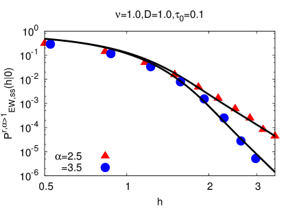
Figure 1: Steady-state height distribution for the $1d$ EW interface subject to resetting at power-law times, with $\alpha>1.$ The points refer to numerical simulations of a discrete interface of size $L=2^{14}$, while lines refer to the exact result (11). The various parameter values are indicated in the figure.

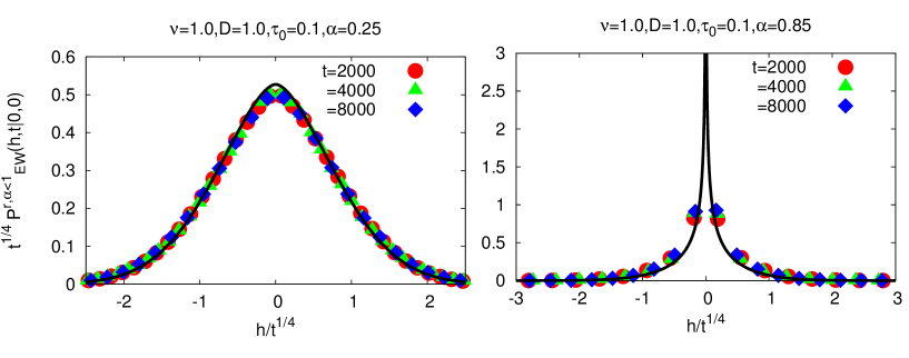
Figure 2: Time-dependent height distribution for the $1d$ EW interface subject to resetting at power-law times, with $\alpha<1.$ The data points are obtained from numerical simulations of a discrete interface of size $L=2^{14}$. Collapse of the data for different times follows the scaling form (21), with $\beta_{\rm EW}=1/4$. Here, the lines denote the exact scaling function (22).

3 Predictions for a general interface

Consider now a general interface characterized by scaling exponents $\chi,z$, and $\beta=\chi/z$, for which the distribution $P(h,\tau|0,0)$ in the limit $\tau\to\infty,|h|\to\infty$, keeping $|h|/\tau^{\beta}$ fixed and finite, has the scaling form $P(h,\tau|0,0)\sim(1/\tau^{\beta})g\left(h/\tau^{\beta}\right)$, where $g(s)=g(-s)$ is the scaling function. Normalization requires $P(|h|\to\infty,\tau|0,0)\to 0~{}\forall~{}\tau$. Provided the interface dynamics is Markovian in the full configuration space, Eq. (5) will still hold for such an interface.

3.1 Height distribution for $\alpha>1$

Using Eq. (5) and the expression for $f_{\alpha>1}(t,t-\tau)$, we get

$$P^{{\rm r},\alpha>1}(h,t|0,0)=P(h,\tau_{0}|0,0)\left[\frac{\alpha-1}{\alpha}+\frac{1}{\alpha}\Big{(}\frac{t}{\tau_{0}}\Big{)}^{1-\alpha}\right]$$

$$+\int_{\tau_{0}}^{t}d\tau~{}\frac{1}{\,\tau_{0}}\Big{(}\frac{\alpha-1}{\alpha}\Big{)}\Big{(}\frac{\tau}{\tau_{0}}\Big{)}^{-\alpha}P(h,\tau|0,0).$$ (30)

The stationary state, obtained in the limit $t\to\infty$, has the large-$h$ behavior given by $P_{{\rm ss}}^{{\rm r},\alpha>1}(|h|\to\infty|0)\sim\int_{\tau^{\star}}^{\infty}d\tau~{}(1/\tau^{\alpha+\beta})g(|h|/\tau^{\beta})$, where $\tau^{\star}$ is such that the scaling form for $P(h,\tau|0,0)$ holds for $\tau>\tau^{\star}$, and we have used the smallness of $\tau_{0}$ to neglect the contribution of $P(h,\tau_{0}|0,0)$ as $|h|\to\infty$. The above equation implies a power-law decay of the height distribution at the tails,

$$P_{{\rm ss}}^{{\rm r},\alpha>1}(|h|\to\infty|0)\sim\frac{1}{|h|^{(\alpha+\beta-1)/\beta}},$$ (31)

which therefore predicts a crossover in the interface width, from finite to infinite, at $\alpha^{(\rm w)}=1+2\beta$. These predictions match with our exact results for the EW interface.

3.2 Height distribution for $\alpha<1$

Using Eqs. (5) and (17), we get

$$P^{{\rm r},\alpha<1}(h,t|0,0)=\int_{0}^{t}d\tau~{}\tau^{-\alpha}(t-\tau)^{\alpha-1}P(h,\tau|0,0),$$ (32)

so that for large $t$, one has the large-$h$ behavior $P^{{\rm r},\alpha<1}(|h|\to\infty,t\to\infty|0,0)\sim\int_{\tau^{\star}}^{t}d\tau~{}\tau^{-(\alpha+\beta)}(t-\tau)^{\alpha-1}g(|h|/\tau^{\beta})$, where $\tau^{\star}$ is such that the scaling form for $P(h,\tau|0,0)$ holds for $\tau>\tau^{\star}$. One then arrives at the scaling form

$$P^{{\rm r},\alpha<1}(h,t|0,0)\sim\frac{1}{t^{\beta}}g_{\rm r}\Big{(}\frac{h}{t^{\beta}}\Big{)},$$ (33)

consistent with the result (21) obtained for the EW interface. In the paragraph following Eq. (29), we have already discussed that close to the resetting location, $P^{{\rm r},\alpha<1}(h,t|0,0)$ is expected to exhibit a crossover in behavior, from cusp to divergence, across $\alpha^{(\rm d)}=1-\beta$.

3.3 Numerical simulations for a KPZ interface

Our derived predictions for the different behaviors of fluctuations are summarized in Table 1; to confirm their validity beyond the EW interface, we now consider a $1d$ periodic interface in the KPZ universality class. In this case, the evolution equation (1) is augmented by a non-linear term:

$$\frac{\partial H}{\partial t}=\nu\frac{\partial^{2}H}{\partial x^{2}}+\frac{\lambda}{2}\Big{(}\frac{\partial H}{\partial x}\Big{)}^{2}+\eta(x,t),$$ (34)

and the exponents $z,\chi,\beta$ have the values $z_{{\rm KPZ}}=3/2,\chi_{{\rm KPZ}}=1/2,\beta_{{\rm KPZ}}=1/3$. To check our predictions, we performed numerical simulations of a discrete $1d$ periodic interface $\{H_{i}(t)\}_{1,2,\ldots,L}$, which evolves in discrete times $t$ according to the following dynamics of the ballistic deposition model in the KPZ universality class [20, 21, 22],

$$H_{i}(t+1)={\rm max}[H_{i-1}(t),H_{i}(t)+1,H_{i+1}(t)],$$ (35)

and is additionally reset to the initial flat configuration $H_{i}(0)=0~{}\forall~{}i$. As in all our discussions in this paper, we take two successive resets to be separated by a random interval $\tau$ sampled from the power-law distribution (3). The results of numerical simulations shown in Figs. 3 and 4 are fully consistent with the predictions in Table 1.

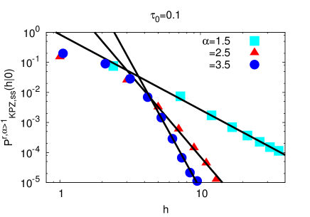
Figure 3: Steady-state height distribution for the $1d$ KPZ interface subject to resetting at power-law times, with $\alpha>1.$ The points refer to numerical simulations of a discrete interface of size $L=2^{14}$, while lines refer to the predicted power-law tails, Eq. (31).

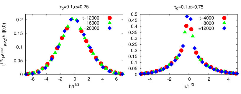
Figure 4: Time-dependent height distribution for the $1d$ KPZ interface subject to resetting at power-law times, with $\alpha<1.$ The data points are obtained from numerical simulations of a discrete interface of size $L=2^{14}$. Collapse of the data for different times follows the scaling (33) with $\beta=\beta_{\rm KPZ}=1/3$.

4 Conclusions

In this work, we studied the problem of a fluctuating interface in one dimension, whose dynamics is interrupted with resetting to a given initial configuration, namely, a flat configuration, after random time intervals $\tau$ distributed as a power-law $\sim\tau^{-(1+\alpha)};~{}\alpha>0$. With respect to an earlier study that considered resetting at exponential times [19], here we demonstrated by exact analytical results and numerical simulations that the dynamics exhibits new and interesting reset-induced effects, including many crossover phenomena. We found that the distribution of interface fluctuations $h$ is time dependent for $0<\alpha<1$, and, moreover, the distribution around the resetting value $h=0$ shows a crossover from a cusp for $\alpha<\alpha^{({\rm d})}$ to a divergence for $\alpha^{({\rm d})}<\alpha<1$, where $\alpha^{({\rm d})}\equiv 1-\beta$. The interface width grows with time as $t^{\beta}$, which is also the situation in the absence of resetting. For $\alpha>1$, by contrast, the distribution of fluctuations is time independent, yet the interface width diverges with time for $1<\alpha<\alpha^{({\rm w})}$, but is time independent with a finite value for $\alpha>\alpha^{({\rm w})}$, with $\alpha^{({\rm w})}\equiv 1+2\beta$. These features may be contrasted with resetting at exponentially-distributed times that always leads to a time-independent state at long times with a finite value of the interface width [19].

The qualitative behaviors and the cross-overs observed here for the many-body interacting system of an interface were previously reported by us to be present also for a single particle undergoing stochastic resetting at power-law times [19], and their origin may be traced to the form of the probability $f_{\alpha}(t,t-\tau)$, Eqs. (6) and (17), a vital ingredient in determining the behavior of fluctuations for either system, and, thence, essentially to the properties of the resetting time distribution $\rho(\tau)$, Eq. (3). Indeed, for $0<\alpha<1$, the presence of fluctuations that are unbounded in time (so that there is no stationary state even at long times) is due to the fact that for this range of $\alpha$, the average gap $\langle\tau\rangle$ between successive resets is infinite, so that there are only a small number of reset events in a given time, and in between the fluctuations may grow unbounded in time. The situation is very different for $\alpha>1$; in this case, a finite $\langle\tau\rangle$ implies frequent resets in a given time, so that the fluctuations cannot grow unbounded in time, and hence, the dynamics exhibits a long-time stationary state. This physical picture was proposed and validated by us in the context of a single diffusing particle in Ref. [5], and the present work demonstrates its generality beyond a single particle to a many-interacting particle system. Besides the example of a fluctuating interface, it would be interesting to study if and how resetting leads to new behaviors in other many-particle interacting systems, such as models of interacting particles diffusing on a lattice.

References

• [1] M. R. Evans and S. N. Majumdar, Phys. Rev. Lett. 106, 160601 (2011).
• [2] S. N. Majumdar, S. Sabhapandit, and G. Schehr, Phys. Rev. E 91, 052131 (2015).
• [3] S. Reuveni, arXiv:1512.01600.
• [4] S. Eule and J. J. Metzger, New J. Phys. 18, 033006 (2016).
• [5] A. Nagar and S. Gupta, arXiv:1512.02092 (Submitted).
• [6] C. Christou and A. Schadschneider, J. Phys. A: Math. Theor. 48, 285003 (2015).
• [7] A. Pal, Phys. Rev. E 91, 012113 (2015).
• [8] M. R. Evans and S. N. Majumdar, J. Phys. A: Math. Theor. 44, 435001 (2011).
• [9] D. Boyer and C. Solis-Salas, Phys. Rev. Lett. 112, 240601 (2014).
• [10] S. N. Majumdar, S. Sabhapandit, and G. Schehr, Phys. Rev. E 92, 052126 (2015).
• [11] M. Montero and J. Villarroel, Phys. Rev. E 87, 012116 (2013).
• [12] V. MΓ©ndez and D. Campos, Phys. Rev. E 93, 022106 (2016).
• [13] L. Kusmierz, S. N. Majumdar, S. Sabhapandit, and G. Schehr, Phys. Rev. Lett. 113, 220602 (2014).
• [14] D. Campos and V. MΓ©ndez, Phys. Rev. E 92, 062115 (2015).
• [15] A. Pal, A. Kundu, and M. R. Evans, arXiv:1512.08211.
• [16] X. Durang, M. Henkel, and H. Park, J. Phys. A: Math. Theor. 47, 045002 (2014).
• [17] Γ‰. RoldΓ‘n, A. Lisica, D. SΓ‘nchez-Taltavull, and S. W. Grill, arXiv:1603.06956.
• [18] J. Fuchs, S. Goldt, and U. Seifert, EPL 113, 60009 (2016).
• [19] S. Gupta, S. N. Majumdar, and G. Schehr, Phys. Rev. Lett. 112, 220601 (2014).
• [20] A.-L. BarabΓ‘si and H. E. Stanley, Fractal Concepts in Surface Growth (Cambridge University Press, Cambridge, England, 1995).
• [21] T. Halpin-Healy and Y. C. Zhang, Phys. Rep. 254, 215 (1995).
• [22] J. Krug, Adv. Phys. 46, 139 (1997).
• [23] S. F. Edwards and D. R. Wilkinson, Proc. R. Soc. Lond. A 381, 17 (1982).
• [24] For a translationally invariant interface, one has $\langle h\rangle=0$.
• [25] F. Family and V. Vicsek, J. Phys. A 18, L75 (1985).
• [26] Anomalous Transport: Foundations and Applications, edited by R. Klages, G. Radons, and I. M. Sokolov (Wiley-VCH, Weinheim, 2008).
• [27] M. Kardar, G. Parisi, and Y.-C. Zhang, Phys. Rev. Lett. 56, 889 (1986).
• [28] A. J. Bray, S. N. Majumdar, and G. Schehr, Adv. Phys. 62, 225 (2013).
• [29] C. GodrΓ¨che and J. M. Luck, J. Stat. Phys. 104, 489 (2001).
• [30] We use Γ​(a,x)=Γ​(a)​[1βˆ’xa​exp⁑(βˆ’x)β€‹βˆ‘k=0∞xk/Γ​(a+k+1)];aβ‰ 0,βˆ’1,βˆ’2,…formulae-sequenceΞ“π‘Žπ‘₯Ξ“π‘Ždelimited-[]1superscriptπ‘₯π‘Žπ‘₯superscriptsubscriptπ‘˜0superscriptπ‘₯π‘˜Ξ“π‘Žπ‘˜1π‘Ž012…\Gamma(a,x)=\Gamma(a)\Big{[}1-x^{a}\exp(-x)\sum_{k=0}^{\infty}x^{k}/\Gamma(a+k+1)\Big{]};~{}a\neq 0,-1,-2,\ldots [31].
• [31] NIST Handbook of Mathematical Functions, edited by F. W. J. Olver, D. W. Lozier, R. F. Boisvert, and C. W. Clark (Cambridge University Press, New York, 2010).
• [32] Here, one uses the results [31] $\int_{0}^{\infty}dy~{}y^{2k+2}\exp(-y^{2})=\Gamma(k+3/2)/2$ for $k+3/2>0,$ $\sum_{k=0}^{\infty}\Gamma(2\alpha-3/2)\Gamma(k+3/2)/\Gamma(2\alpha-1/2+k)=\sqrt{\pi}/[2(2\alpha-3)]$.
• [33] In the limit $|x|\to\infty$, it is known that [34] $G_{p,q}^{q,0}(\begin{array}[]{c}a_{p}\\ b_{q}\end{array}|x)\approx(2\pi)^{(\sigma-1)/2}/\sqrt{\sigma}\exp(-\sigma x^{1/\sigma})x^{\theta}$, with $|{\rm arg}~{}x|\leq(\sigma+\epsilon)\pi-\delta$, $\delta>0$, and $\sigma\equiv q-p$, where $\epsilon=1/2$ if $\sigma=1$ and $\epsilon=1$ if $\sigma>1$, while $\sigma\theta=(1/2)(1-\sigma)+\sum_{h=1}^{q}b_{h}-\sum_{h=1}^{p}a_{h}$. On the other hand, as $x\to 0$, we have [35] $x^{-a}\Big{(}\Big{(}\frac{\sqrt{\pi}\Gamma(\frac{3}{4}-a)}{\Gamma\left(\frac{3}{4}\right)}-\frac{2\left(\sqrt{\pi}\Gamma\left(\frac{1}{4}-a\right)\right)\sqrt{x}}{\Gamma\left(\frac{1}{4}\right)}+\frac{2\sqrt{\pi}\Gamma\left(\frac{3}{4}-a\right)x}{(4a+1)\Gamma\left(\frac{3}{4}\right)}+O\left(x^{3/2}\right)\Big{)}x^{a}+\left(\frac{\Gamma\left(a-\frac{3}{4}\right)\Gamma\left(a-\frac{1}{4}\right)x^{3/4}}{\Gamma(a)}+O\left(x^{5/4}\right)\right)\Big{)}$.
• [34] The Special Functions and their Approximations, Y. L. Luke (Academic Press, London, 1969).
• [35] E. W. Weisstein, β€œMeijer G-Function.” From MathWorld–A Wolfram Web Resource. http://mathworld.wolfram.com/MeijerG-Function.html
• [36] For a general interface also, we have $P(h\to 0,\tau>0|0,0)$ = a finite constant. Indeed, even on starting with a flat interface, so that $P(h,0|0,0)=\delta(h)$, the dynamical evolution will roughen the interface in a finite time, so that $P(h,\tau>0|0,0)$ will have a finite width, and in particular, will result in $P(h\to 0,\tau>0|0,0)$ = a finite constant.