The data, they are a-changin’

Abstract

The cost of deriving actionable knowledge from large datasets has been decreasing thanks to a convergence of positive factors: low cost data generation, inexpensively scalable storage and processing infrastructure (cloud), software frameworks and tools for massively distributed data processing, and parallelisable data analytics algorithms. One observation that is often overlooked, however, is that each of these elements is not immutable, rather they all evolve over time. This suggests that the value of such derivative knowledge may decay over time, unless it is preserved by reacting to those changes. Our broad research goal is to develop models, methods, and tools for selectively reacting to changes by balancing costs and benefits, i.e. through complete or partial re-computation of some of the underlying processes. In this paper we present an initial model for reasoning about change and re-computations, and show how analysis of detailed provenance of derived knowledge informs re-computation decisions. We illustrate the main ideas through a real-world case study in genomics, namely on the interpretation of human variants in support of genetic diagnosis.

1 Introduction

One simple but rarely addressed observation in Data Science is that many of the large datasets used to derive knowledge, i.e. through “Big Data” computations, evolve over time. This causes problems as changes in the datasets invalidate some of the insight derived from them. This is true for instance for the large class of predictive models generated using statistical inference (i.e. machine learning algorithms), whose accuracy when used in the wild tends to decay as the assumptions embodied by the data used for training are no longer valid. This problem is also relevant in data-intensive science, where experimental results often come from computational pipelines or simulations that rely on observational data. In these settings, not only the underlying data, but also the algorithms, external reference data sources used in the analysis, as well as other dependencies evolve continuously. These changes may represent both a threat, i.e. when a stale model is used to make decisions, and an opportunity, namely to upgrade derived knowledge by performing the analysis again. When the processes are computationally expensive and the available budget for re-doing old work is limited, it is important to be able to determine when re-computation, partial or complete, of the underlying analytic tasks in reaction to changes is beneficial.

The potential for exploiting provenance records for partial re-computation has been studied before, in the specific context of database operations. In the Panda system Ikeda et al. [2011]; Ikeda and Widom [2010], for instance, one can determine precisely the fragment of a data-intensive program that needs to be re-executed in order to refresh stale results. However, this requires the assumption that very granular data provenance can be collected for database operations, and that the semantics of these operations is well understood.

In contrast, in this paper we take a broader view and consider a scenario where (i) the computation involves any program $P$ that has dependencies on external data resources, (ii) the program structure and details of its execution may be only partially observable (coarse vs fine-grained provenance), and (iii) the program may have been executed many times over many inputs, producing a (large) history $H$ of past computations and results.

We note that changes in the content of the external resources may invalidate some, but not all, of the results in $H$. Furthermore, as noted in the Panda system, when attempting to refresh the results that are affected, it may be possible to re-compute $P$ only partially. In this paper we show how provenance records from past computations, of varying granularity, can be used to select the precise subset of $H$ that becomes invalid when the content of external resources changes (re-comp scope). We also show how the starting point for a partial re-computation of $P$ can be pinpointed.

Our specific contributions are as follows: (i) a formalisation of a re-computation framework under our assumptions, (ii) a discussion of the role of provenance and of how granular provenance translates into efficient re-computation through precise selection of the re-comp scope, and (iii) an illustration of the framework in action on a real-world process of analysis of human genetic variants.

This initial investigation is part of a larger project, ReComp, which aims to offer models for estimating the impact of changes in input and external data on the outcome of a program, in order to prioritise re-computation over the affected population vis-à-vis a limited budget.

Related Work.

As mentioned, the Panda prototype system Ikeda et al. [2011] aims at collecting and exploiting provenance to enable data refresh, by selecting the fragments of a data-intensive workflow that must be re-executed. The focus here is on white box computations which involve database operations, which are documented using perfect and granular provenance records, and we have already commented on the broader and less rigid scope of our work. A formal definition of correctness and minimality of a provenance trace with respect to a data-oriented workflow is proposed by members of the same group Ikeda et al. [2013], leading to a notion of logical provenance. Although this may become a potentially useful building block for a future version of this work, it completely ignores the PROV data model Moreau et al. [2012] which, instead, we regard as a practical foundation to enable interoperability of any provenance-based re-computation framework.

A similar perspective to Panda is taken in the Archived Metadata and Provenance Manager (AM&PM) Gao and Zaniolo [2012], with a focus on database provenance and where the main evolving element is not the data but the database schema. Accordingly, the provenance of schema evolution is captured and can be queried, along with the provenance of the data in the current and past versions of a database. Interestingly, using a schema evolution language (Prism Curino et al. [2008]) leads to a formal definition of what in this paper we call a $\mathit{diff}$ function, aimed at quantifying the difference between two schemas. That research is vaguely related to our work, which does not specifically address database operations placing schema evolution out of scope.

Finally, as an infrastructure mechanism to enable selective recomputation, the strong links approach of Koop et al. [2010] is relevant in this context.

Figure 1: Increase in the count of genes (left) and variants (right) over time, related to diseases affecting a cohort of patients at the IGM, Newcastle.

Example: analysis of human genetic variants.

To illustrate the problem addressed in the rest of this paper, we consider a use case consisting of a process called Simple Variant Interpretation (SVI). SVI is a tool we have developed as part of the Cloud-eGenome project Missier et al. [2015], aimed at providing a simple interpretation of human variants to facilitate clinical diagnosis of genetic diseases. Here a variant is a single nucleotide mutation that occurs on a gene. Variants are identified by processing a patient’s genome (or their exome, a small portion of the genome) using a sequence of algorithmic steps that, essentially, compare it to a reference genome. SVI takes a set of variants found in the patient’s exome (about 25,000) and a set of terms that describe the patient’s phenotype, which indicates the patient’s disease hypothesis (presumed disorder). It selects a small subset of the variants which are relevant for the phenotype, and associates a degree of estimated deleteriousness to each of them. To do this it uses knowledge from external data resources, namely the ClinVar and OMIM Gene Map databases, described in more detail later.

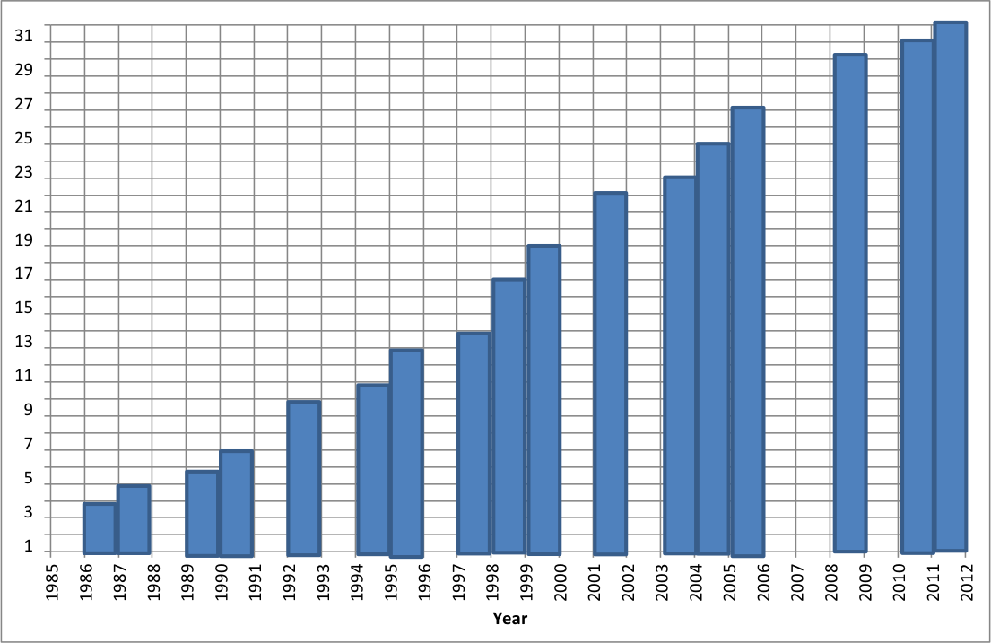
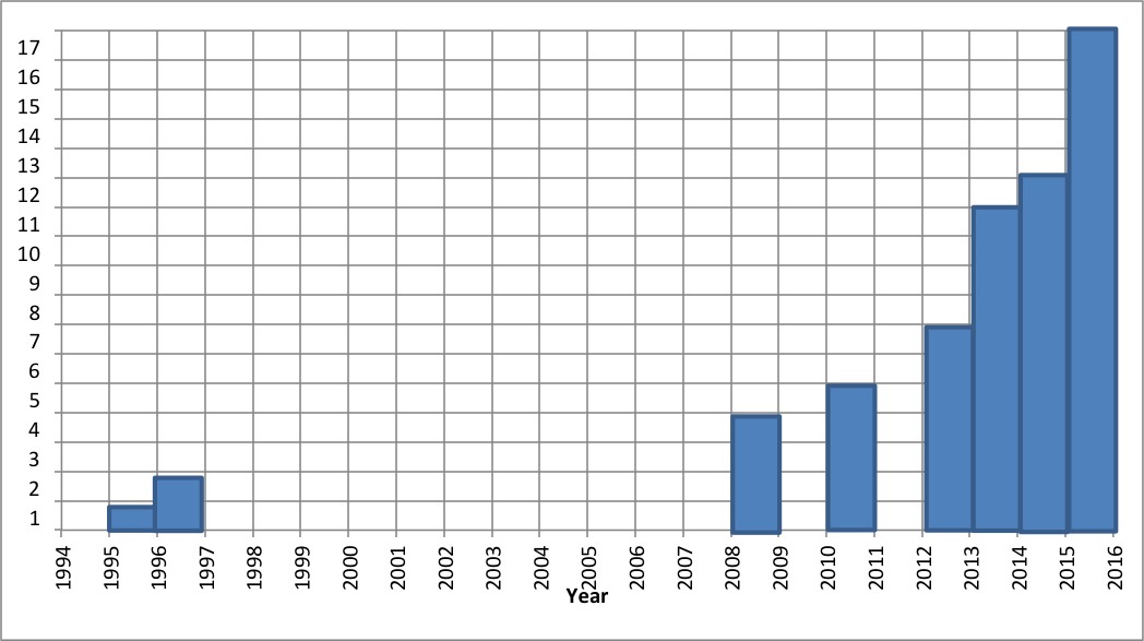
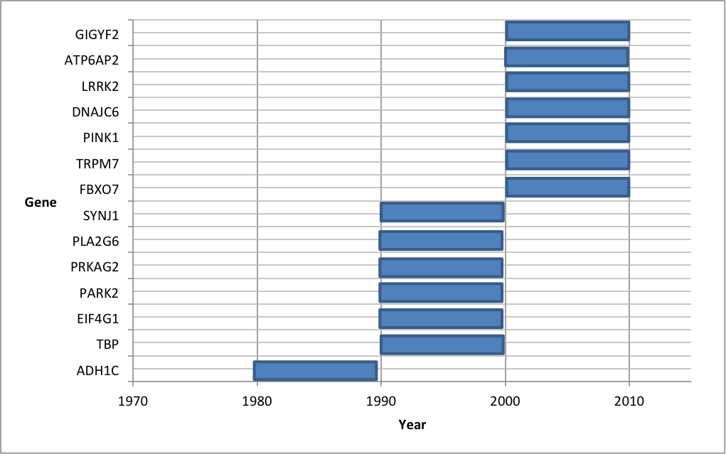
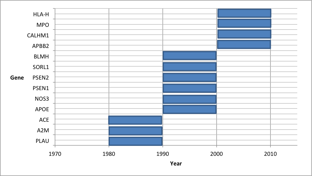
In some cases, the presence of deleterious variants represents conclusive evidence in support of the disease hypothesis. More often, however, the diagnosis is not conclusive due to missing information about the variants, or to lack of knowledge about the association between the hypothesis and the variants. Thus, the diagnostics conclusions that can be drawn from the data are very much dependent on the content of these reference databases which encode the current genetic knowledge. As this knowledge evolves and these resources are updated, there are opportunities to revisit past inconclusive diagnoses, and thus to consider re-computation of the associated analysis. To appreciate the effect of changes in the reference knowledge, in Fig. 1 we show how new additions to the OMIM and ClinVar databases would have affected the ability to carry out a conclusive diagnosis on a cohort of patients seen at the Institute of Genetic Medicine (IGM) in Newcastle. The charts show the number of genes and variants within a gene, respectively, known to researchers and which would have been relevant for those patients. The charts in Fig. 2 provide a similar view of the evolution over time of the genes known to be implicated in specific diseases, namely Parkinson’s and Alzheimer’s.

Figure 2: Progressive increase in the count of genes known to be involved in Parkinson’s and Alzheimer’s over time, in the OMIM Gene Map database.

The ReComp problem in this use case involves (i) selecting the cases that are likely to benefit from re-computation, (ii) deciding whether complete or partial re-computation is required, and (iii) actually reproducing the original process, possibly requiring a new deployment.

2 Re-computation framework

To frame the re-computation decision problem in simple, abstract terms we present the set of basic elements that ReComp is built upon.

Computation.

Consider program $P$ executing on a set $\mathbf{x}=\{x_{1}\ldots x_{n}\}$ of inputs and producing outputs $\mathbf{y}=\{y_{1}\dots y_{m}\}$, which also makes use of external data resources, or data dependencies $\mathbf{D}=\{D_{1}\ldots D_{m}\}$ where each $D_{i}$ is a dataset, $D_{i}=\{d_{i1},d_{i2}\dots\}$. We also associate a version $v$ to each execution. This indicates a timestamp and uniquely identifies one execution of $P$, denoted by:

$$\mathbf{y}^{v}=P^{v}(\mathbf{x}^{v}|\mathbf{D}^{v})$$ (1)

Transparency.

The level of detail available in observing a computation of $P$ (the transparency of $P$) plays an important role in making re-computation decisions. We consider two aspects of transparency, namely (a) details on the internal structure of $P$, and (b) details on which subset of each $D_{i}$ are used. At one end of the “transparency spectrum”, no details are available for either (a) or (b): $P$ is a black box providing no details about its internal structure, and all we know about $D_{i}$ are coarse-grain statements like “ClinVar was used at some point”. On the opposite end of the spectrum, $P$ is a white-box, described for instance $P$ by function composition $P\equiv P_{r}\circ\ldots\circ P_{1}$. At the same time, we also understand the semantics of each subprocess $P_{j}$ and know the subset of $D_{i}$ that was used by a $P_{j}$.

Provenance.

The provenance of an output $\mathbf{y}$, denoted $\mathit{prov}(\mathbf{y})$, is a PROV document that describes the derivation of $\mathbf{y}$ from $\mathbf{x}$ through $P$ using elements of $\mathbf{D}$. The granularity of PROV assertions may differ depending on the transparency of $P$. In the most granular case, when $P$ is a white box we can for instance express the usage of any single element $d_{ij}\in D_{i}\in\mathbf{D}$ by an activity $P_{j}$, i.e. using statements of the form:

$$\small\texttt{used}(P_{j},d_{ij},[\texttt{prov:role}=\texttt{'dep'}])$$ (2)

where the role indicates that $d_{ij}$ is a dependency. Similarly, for inputs $x_{i}$ (or intermediate values) we can write:

$$\small\texttt{used}(P_{j},x_{i},[\texttt{prov:role}=\texttt{'input'}])$$ (3)

At the other extreme, in a completely black box scenario, the assertions will be of the form:

$$\texttt{used}(P,\mathbf{D},[\texttt{prov:role}=\texttt{'dep'}])\text{ (use of dependency) }$$ (4)

$$\texttt{used}(P,\mathbf{x},[\texttt{prov:role}=\texttt{'input'}])\text{ (use of input) }$$ (5)

In addition to producing $\mathit{prov}(\mathbf{y})$, each computation of form (1) also generates history record $h$:

$$h(\mathbf{y},v)=\langle P^{v},\mathbf{D}^{v},\mathbf{x}^{v},\mathit{prov}(\mathbf{y}^{v}),\mathit{cost}(\mathbf{y}^{v})\rangle$$ (6)

where it is expected that $\mathit{prov}(\mathbf{y}^{v})$ contains statements that make references to $P^{v}$, $\mathbf{x}^{v}$, and $\mathbf{D}^{v}$. Over time, statements of the form (6) form a History database $\mathit{H}$. Note that we also record the $\mathit{cost}(\mathbf{y})$ of computing $\mathbf{y}$ by executing $P$ on $\mathbf{x}$. Although the specific form of the cost is immaterial here, in practice it can be expressed as a monetary cost (e.g. when $P$ is executed on a public cloud), execution time, resource usage or as a combination of them.

Change detection.

ReComp relies on the capability to detect and quantify changes between any two versions of $\mathbf{x}$ and $\mathbf{D}$, i.e. $\mathbf{x}^{v}\rightarrow\mathbf{x}^{v^{\prime}}$, $\mathbf{D}^{v}\rightarrow\mathbf{D}^{v^{\prime}}$. Thus, we assume there exist three families of diff functions that are needed to compare two versions of the elements of $\mathbf{x}$, $\mathbf{D}$, and $\mathbf{y}$.

input diff: $$\{\mathit{diff}_{in}(x_{i}^{v},x_{i}^{v^{\prime}})|x^{v}_{i}\in\mathbf{x}^{v},x^{v^{\prime}}_{i}\in\mathbf{x}^{v^{\prime}}\}$$

dependency diff: $$\{\mathit{diff}_{d}(D_{i}^{v},D_{i}^{v^{\prime}})|D^{v}_{i}\in\mathbf{D}^{v},D^{v^{\prime}}_{i}\in\mathbf{D}^{v^{\prime}}\}$$

output diff: $$\{\mathit{diff}_{out}(y_{i}^{v},y_{i}^{v^{\prime}})|y^{v}_{i}\in\mathbf{y}^{v},y^{v^{\prime}}_{i}\in\mathbf{y}^{v^{\prime}}\}$$

These operate independently on each input, dependency, and output component. Each of these functions will have a different signature, and produce a summary of changes found in its inputs, in a format that may vary depending on the types of $\mathbf{x}$ and $\mathbf{D}$. For instance, $\mathit{diff}_{d}(D_{i}^{v},D_{i}^{v^{\prime}})$ typically computes the symmetric difference $(D_{i}^{v}\setminus D_{i}^{v^{\prime}})\cup(D_{i}^{v^{\prime}}\setminus D_{i}^{v})$. Other types of diff functions can be defined for specific use cases. Note that, although changes in the structure of program $P$ are also relevant and are within the general ReComp framework, for simplicity in this short contribution we are going to assume that $P$ does not change.

Role of the $\mathit{H}$ database and of provenance.

As mentioned earlier, upon detecting changes (i.e. using the diff functions) the first steps in making re-computation decisions include (i) scoping rules, that is selecting the subset $H^{\prime}\subset H$ of the computations described in $H$ that are affected by these changes, and (ii) defining the starting point $P_{s}$ of a partial re-computation of $P$, which we call the starting component of $P$. This is the component of $P$ mentioned in the earliest usage of a changed dataset (input or dependency), and it is not necessarily the same as the start of the whole of $P$. Note that partial re-computation is only possible if the input to $P_{s}$ is available, i.e. not only should the input be explicitly mentioned in $\mathit{prov}(\mathbf{y})$, but it must also have been cached in a data store.

In a white box scenario where $P$’s executions are fully observable, both steps can be addressed by querying the provenance documents in $\mathit{H}$. We distinguish the case of a change in inputs $\mathbf{x}$ from the case of a change in a dependency $D_{i}\in\mathbf{D}$. These correspond to the two patterns (3) and (2) above. Specifically, if the change $x_{i}^{v}\rightarrow x_{i}^{v^{\prime}}$ involves any of the inputs $x_{i}\in\mathbf{x}$, the scope $H^{\prime}$ is simply the set of records $h$ in which $x_{i}^{v}$ is used as input, i.e. all $h(\mathbf{y},v)$ such that $\mathit{prov}(\mathbf{y}^{v})$ includes the pattern of form (3).

Regarding dependency change $D_{i}^{v}\rightarrow D_{i}^{v^{\prime}}$, the affected records are those where the computation involved elements in $\mathit{diff}_{d}(D_{i}^{v},D_{i}^{v^{\prime}})$. These are the $h(\mathbf{y},v)$ such that: (i) $\mathit{prov}(\mathbf{y}^{v})$ includes the pattern of form (2) involving data element $d_{ij}$, and (ii) $d_{ij}\in\mathit{diff}_{d}(D_{i}^{v},D_{i}^{v^{\prime}})$.

Next, within the scope determined as above, we need to determine the starting component $P_{s}$ of each $P$. The provenance patterns just mentioned, (3) and (2), provide the answer, namely the starting component is the activity $P_{j}$ that appears in the earliest occurrence of a usage statement involving a changed input or dependency.

Finally, note that in a black box scenario, with either limited visibility of process structure and/or of data input granularity, the scoping rules cannot be used, i.e. the default scope is the whole of $H$, and total (as opposed to partial) re-computation of $P$ is required.

Figure 3: White box SVI, with inputs $\mathbf{x}=[\mathit{varset},\mathit{ph}]$ and data dependencies $\mathbf{D}=[\text{OMIM},\text{ClinVar}]$

3 Detailed use case: SVI re-computation

We now illustrate the framework in use on our SVI case study. One execution of SVI, illustrated in Fig. 3, is carried out for each patient whose diagnosis we want to confirm. SVI is an example of process $P$ with inputs:

$$\mathbf{x}=[\mathit{varset},\mathit{ph}]$$

where $\mathit{varset}$ is the set of variants associated with the patient, and $\mathit{ph}=\{\mathit{dt}_{1},\mathit{dt}_{2},\dots\}$ is the phenotype expressed using disease terms $\mathit{dt}_{i}$ from the OMIM vocabulary, for example Alzheimer’s. SVI is a classifier that associates a class label to each input variant depending on their estimated deleteriousness, using a simple “traffic light” notation, i.e.:

$$\mathbf{y}=\{(v,\mathit{class})|v\in\mathit{varset},\mathit{class}\in\{\textsf{red},\textsf{amber},\textsf{green}\}\}$$

The amber variants are typically the majority, indicating uncertain diagnosis, while one or two red (pathogenic) variants are sufficient to complete the diagnosis.

SVI’s data dependencies $\mathbf{D}$ consist of the two reference databases, OMIM and Clinvar, each subject to periodic revisions and denoted $\mathbf{D}^{v}=[\mathit{OM^{v}},\mathit{CV^{v}}]$. OMIM maintains a vocabulary $\mathit{DT}$ of standard terms used to denote human disorders. To each of these terms, OMIM associates a set of genes that are known to be broadly involved in the disease. We denote the mapping from $\mathit{dt}\in\mathit{DT}$ to genes via $\mathit{OM^{v}}$ as $\mathit{genes}\ (\mathit{dt},\mathit{OM^{v}})$. ClinVar contains catalogue $V$ of single-nucleotide human variants, and it is used to try and determine the clinical significance of the genetic mutations in patients, i.e. those variants found in $\mathit{varset}$. Specifically, Clinvar associates a status to each variant $\mathit{var}\in V$, denoted $\mathit{varstatus}(\mathit{var},\mathit{CV^{v}})\in\{\textsf{unknown},\textsf{benign},\textsf{pathogenic}\}$.

SVI uses versions $\mathit{OM^{v}}$ and $\mathit{CV^{v}}$ of OMIM and ClinVar to investigate a patient’s disease, as shown in Fig. 3. Firstly, the terms in $\mathit{ph}$ are used to determine the set of target genes that are relevant for the disease hypothesis. These are defined as the union of all the genes in $genes(\mathit{dt},\mathit{OM^{v}})$ for each disease term $\mathit{dt}\in\mathit{ph}$. For example, if the patient’s phenotype is Alzheimer’s, then genes like PSEN2 and PLAU are in scope, but for instances a gene that is known to be implicated in Parkinson’s disease, such as PARK2, will not be considered in the investigation.

Secondly, a subset of the variants in $\mathit{varset}$ is selected, according to standard filtering rules; variant $\mathit{var}\in\mathit{varset}$ is selected if it is located on the target genes. And, finally, the variants are classified as red, amber, or green depending on $\mathit{varstatus}(\mathit{var},\mathit{CV^{v}})$ (variants that are not catalogued at all in ClinVar become amber).

To illustrate the process consider two patients from the IGM cohort mentioned briefly in the introduction. Patient 1 is diagnosed with Alzheimer’s, while Patient 2 is presumably affected by Parkinson’s. Since the ’90s, two genes have been known to be loosely implicated in these diseases, PSEN2 and PARK2, respectively:

$$\texttt{PSEN2}\in\mathit{genes}\ (\texttt{Alzheimer's},\mathit{OM^{1995}}),$$

$$\texttt{PARK}\in\mathit{genes}\ (\texttt{Parkinson's},\mathit{OM^{1995}})$$

However, it was not until 2015 that two specific variants situated on those genes, at position 227083249 and 161807855, respectively have been studied and added to ClinVar. Thus, until 2014 we had

$$\mathit{varstatus}(227083249,\mathit{CV^{2014}})=\textsf{amber},$$

$$\mathit{varstatus}(161807855,\mathit{CV^{2014}})=\textsf{amber}$$

because neither variants were known to ClinVar.

Diff functions.

For OMIM, $\mathit{diff}_{OM}(\mathit{OM^{v}},\mathit{OM^{v^{\prime}}})$ returns the set of terms $t\in T$ for which the mapping to genes has changed:

$$\mathit{diff}_{OM} (\mathit{OM^{v}},\mathit{OM^{v^{\prime}}})=$$

$$\{t\in\mathit{DT}|genes(t,\mathit{OM^{v}})\neq genes(t,\mathit{OM^{v^{\prime}}})\}$$

while $\mathit{diff}_{CV}(\mathit{CV^{v}},\mathit{CV^{v^{\prime}}})$ returns set of variants $\mathit{var}\in V$ with changed status, as well as new variants, or removed variants:

$$\mathit{diff}_{CV} (\mathit{CV^{v}},\mathit{CV^{v^{\prime}}})=$$

$$\{\mathit{var}\in V|\mathit{varstatus}(\mathit{var},\mathit{CV^{v}})\neq\mathit{varstatus}(\mathit{var},\mathit{CV^{v^{\prime}}})\}$$

$$\cup\mathit{CV^{v^{\prime}}}\setminus\mathit{CV^{v}}\cup\mathit{CV^{v}}\setminus\mathit{CV^{v^{\prime}}}$$

Use of provenance.

The provenance from each SVI tool execution is recorded in the $\mathit{H}$ database. Following the white box approach of Sec. 2, the relevant PROV assertions generated from an execution of SVI, with block names as in Fig. 3, are as follows:

$$\texttt{entity}(\texttt{om},[\texttt{prov:type}=\text{'OMIM'},version=\texttt{'v'}])$$ (7)

$$\texttt{entity}(\texttt{ph},[\texttt{prov:type}=\text{'prov:collection'}])$$ (8)

$$\texttt{entity}(\texttt{cv},[\texttt{prov:type}=\text{'CV'},version=\texttt{'v'}])$$ (9)

$$\texttt{entity}(\texttt{vars},[\texttt{prov:type}=\text{'prov:collection'}])$$ (10)

$$\texttt{used}(\texttt{PtG},\texttt{om},[\texttt{prov:role}=\texttt{'dep'}])$$ (11)

$$\texttt{used}(\texttt{PtG},\texttt{ph},[\texttt{prov:role}=\texttt{'input'}])$$ (12)

$$\texttt{used}(\texttt{vClass},\texttt{cv},[\texttt{prov:role}=\texttt{'dep'}])$$ (13)

$$\texttt{used}(\texttt{vClass},\texttt{vars},[\texttt{prov:role}=\texttt{'input'}])$$ (14)

Note that the used assertions are of the form (2) and (3), respectively. These provenance statements can be used to define scoping rules and starting components, as follows.

Re-comp scope due to OMIM changes.

The executions $h$ in the re-comp scope following change $\mathit{OM^{v}}\rightarrow\mathit{OM^{v^{\prime}}}$ include those where phenotype $\mathit{ph}$ includes terms in $\mathit{diff}_{OM}(\mathit{OM^{v}},\mathit{OM^{v^{\prime}}})$, i.e., those with changes to their gene mappings. The phenotype is found in (12), while the version of OMIM for computing diff is found using (11). As (11) contains the earliest mention of om, PtG is also the starting component for re-computation.

Re-comp scope due to ClinVar changes.

Similarly, following change $\mathit{CV^{v}}\rightarrow\mathit{CV^{v^{\prime}}}$, the executions in scope are those that include selected variants on target genes and which appear in $\mathit{diff}_{CV}(\mathit{CV^{v}},\mathit{CV^{v^{\prime}}})$. Using the provenance fragment above, the selected variants are found in (14), and the version of CV for computing diff is found using (13). In this case, vClass is the starting component for re-computation following a change in ClinVar.

Example, continued.

Continuing with our earlier two-patients example, consider again variants 227083249 and 161807855. Because they are both located on genes that have been known to OMIM for many years, these variants are selected as candidates for testing against ClinVar. As mentioned, until 2014 they were both classified as ’amber’. Having been added to ClinVar in 2015, however, they both appear in the latest diff between the 2014 and 2015 versions of ClinVar:

$$\{\texttt{227083249},\texttt{161807855}\}\subset\mathit{diff}_{CV}(\mathit{CV^{2014}},\mathit{CV^{2015}})$$

According to the scoping rule above, the re-comp scope due to these additions includes the executions of $h$ where the provenance mentions 227083249 and 161807855, which include patients 1 and 2 (possibly along with many other patients, but none of those for which these variants are not relevant). As 227083249 is catalogued as “probably pathogenic, uncertain significance”, the diagnosis for patient 1 is still inconclusive. For Patient 2, on the other hand, we can rule out variant 161807855 as a cause of their disease, as this variant is now known to be benign.

4 Conclusions

Knowledge assets derived from data analytics computations may decay and become obsolete as the datasets or the content of reference data resources used to produce it change over time. While this suggests that re-computation of such knowledge assets may be needed, deciding precisely which of them should be re-computed is not a trivial problem; it requires meta-knowledge about their dependencies on the inputs and on the reference datasets.

In this paper we have discussed the role of provenance in providing such meta-knowledge, in a way that can be used to inform re-computation decisions. We have presented a simple reference framework in which data is versioned and functions are available to compute the differences between any two versions. We have clarified how fine-grained and coarse-provenance can be used to assess the impact of such differences on a history of past computations, with different precision, suggesting which past computations should be performed anew. We have illustrated these ideas through a detailed example, concerning the automated classification of human variants for clinical diagnosis.

This work is funded in part by EPSRC grant no. EP/N01426X/1 in the UK.

References

- Curino et al. [2008] C. A. Curino, H. J. Moon, and C. Zaniolo. Graceful Database Schema Evolution: The PRISM Workbench. Proc. VLDB Endow., 1(1):761–772, aug 2008. ISSN 2150-8097. 10.14778/1453856.1453939.
- Gao and Zaniolo [2012] S. Gao and C. Zaniolo. Provenance Management in Databases Under Schema Evolution. Proceedings of the 4th USENIX Conference on Theory and Practice of Provenance, (iii):11, 2012.
- Ikeda and Widom [2010] R. Ikeda and J. Widom. Panda: A system for provenance and data. Proceedings of the 2nd USENIX Workshop on the Theory and Practice of Provenance TaPP’10, 33:1–8, 2010.
- Ikeda et al. [2011] R. Ikeda, S. Salihoglu, and J. Widom. Provenance-based refresh in data-oriented workflows. Proceedings of the 20th ACM international conference on Information and knowledge management, pages 1659–1668, 2011. 10.1145/2063576.2063816.
- Ikeda et al. [2013] R. Ikeda, A. Das Sarma, and J. Widom. Logical provenance in data-oriented workflows? In 2013 IEEE 29th International Conference on Data Engineering (ICDE), pages 877–888. IEEE, apr 2013. ISBN 978-1-4673-4910-9. 10.1109/ICDE.2013.6544882.
- Koop et al. [2010] D. Koop, E. Santos, B. Bauer, M. Troyer, J. Freire, and C. T. Silva. Bridging workflow and data provenance using strong links. In Scientific and statistical database management, pages 397–415. Springer, 2010. ISBN 3642138179.
- Missier et al. [2015] P. Missier, E. Wijaya, R. Kirby, and M. Keogh. SVI: a simple single-nucleotide Human Variant Interpretation tool for Clinical Use. In Procs. 11th International conference on Data Integration in the Life Sciences, Los Angeles, CA, 2015. Springer.
- Moreau et al. [2012] L. Moreau, P. Missier, K. Belhajjame, R. B’Far, J. Cheney, S. Coppens, S. Cresswell, Y. Gil, P. Groth, G. Klyne, T. Lebo, J. McCusker, S. Miles, J. Myers, S. Sahoo, and C. Tilmes. PROV-DM: The PROV Data Model. Technical report, World Wide Web Consortium, 2012.
- Pugh and Teitelbaum [1989] W. Pugh and T. Teitelbaum. Incremental Computation via Function Caching. In Proceedings of the 16th ACM SIGPLAN-SIGACT Symposium on Principles of Programming Languages, POPL ’89, pages 315–328, New York, NY, USA, 1989. ACM. ISBN 0-89791-294-2. 10.1145/75277.75305.