Optimal trading with online parameters revisions

Abstract

The aim of this paper is to explain how parameters adjustments can be integrated in the design or the control of automates of trading. Typically, we are interested by the online estimation of the market impacts generated by robots or single orders, and how they/the controller should react in an optimal way to the informations generated by the observation of the realized impacts. This can be formulated as an optimal impulse control problem with unknown parameters, on which a prior is given. We explain how a mix of the classical Bayesian updating rule and of optimal control techniques allows one to derive the dynamic programming equation satisfied by the corresponding value function, from which the optimal policy can be inferred. We provide an example of convergent finite difference scheme and consider typical examples of applications.

Key words: Optimal trading, market impact, uncertainty, Bayesian filtering.

1 Introduction

The design of trading algorithms is based on two corner stones: first a model need to be estimated, second an optimal trading policy has to be computed, given a prescribed criteria.

As in traditional portfolio management, the notions of volatility or correlation play an important role and need to be estimated. At the level of an order book, one can also be interested by the speed of arrival/cancelation of orders, etc. These refer to the concept of exogenous dynamics, which can be inferred offline, see e.g. [3, 13, 22] for references, and possibly adjusted by using traditional filtering techniques, see e.g. [7, 14].

More importantly, a trading robot has his own impact on the dynamics of the traded assets, either because of market microstructure effects at the high frequency level, or because traded volumes are non-neglectable with respect to the so-called market volume, see [9, 21] for surveys as well as [10] for recent references. The knowledge of this impact is crucial. However, unlike other market parameters, it can be observed only when the algorithm is actually running, offline estimation cannot be done.

As a matter of fact, the controller faces a classical dilemma: should he impulse the system (pass orders) to gain immediately more information to the price of possible immediate losses, or rather try to maximise his current expected reward with the risk of not learning for the future? In any case, the optimal trading policy has to incorporate the fact that the knowledge on the impact parameters will evolve along time, as the effects of the robot on the system are revealed, and that the uncertainty on their value is a source of risk.

One way to analyse this situation is to use the multi-arms bandit recursive learning approach of [19, 20]. By sending successive impulses to the system, one increases his knowledge on the true distribution of the response function. It provides asymptotically optimal policies. The main advantage is that it is model free. On the other hand it requires (weak) ergodicity-type conditions which have little chance to be satisfied if the price/book order is actually impacted. Moreover, the global flow of orders is not optimal, it starts to be optimal only in the long range.

In this paper, we propose to use the classical Bayesian approach, see e.g. [15] for general references. A similar idea has already been suggested in [1] in the context of optimal trading, in a different and very particular framework (trend estimation). In this approach, one fixes an a priori distribution on the true value of the parameters. When a new post-trade information arrives, this distribution is updated according to the Bayesian rule to provide an a posteriori distribution, which will be used as a new prior for the next (bunch of) trade(s). This can, in theory, address pretty general model-free optimal control problems, in the sense that the unknown parameter can be the whole distribution of the response function. Still, the a posteriori distribution will be dominated by the prior. If the true distribution is not, the sequence of estimators cannot converge to it. Also, in practice, computational time constraints will force one to restrict to a class of parameterized distributions, so as to reduce to a space of small dimension. Hence, it requires to choose a set of possible models. Our procedure will only reveal what is the value of the parameters most likely to be, given this prescribed framework. In practice, classes of models are already used by practitioners, but parameters are difficult to estimate at a large scale in an automatic way and evolve according to time and market conditions. From this perspective, we believe that our approach allows us to address their estimation issues in an efficient way.

There are two ways to consider this updating mechanism. One is that it allows one to estimate the true value of the parameters while acting in an optimal manner. This is the point of view developed in [15], who provides conditions for a discrete time infinite horizon model that ensure the convergence of the a posteriori law to the Dirac mass at the true parameter value. Obviously, this requires identification conditions since we can observe the effect on the system only along the optimal policy, as well as some ergodicity conditions. Another point of view is that it actually falls out automatically from dynamic programming considerations when solving the optimal control problem associated to the initial prior.

We focus here on the second point of view: given a prior on the true parameter, how should we act in a optimal way? After all, we want to be optimal given a prior, and not act on the system just to refine the prior if this is not optimal. Obviously, if the algorithm has to be used repeatedly on the same market, and if the conditions on the market are stable, the a posteriori distribution obtained after running the algorithm can be used as a new, more precise, prior for the next time it will be launched. The convergence issue to a Dirac distribution is left for future researches. Again, this is more of academic interest.

We consider here the general abstract formalism introduced in [4] which aims at pertaining for most models used in practice. In particular, we can work at the meta-order level (control of smart-routines) or at the level of single orders (design of smart-routines or scheduling). In the first case, we are interested by the optimal control of robots that are already given, this is similar to [8]. We only observe the global impact of the robot, after it stops. The second case concerns the design of the robots themselves, as in e.g. [2, 16, 19, 20]. A typical question is whether an order should be passive or aggressive. When an aggressive order is posted, we possibly observe an impact immediately (unless it is of small size). As for a (bunch of) limit order(s), we infer the speed at which they have been executed, if they are before being cancelled. The choice of the trading platform can be addressed similarly, etc.

The rest of this paper is organized as follows. After presenting the general framework of [4], we provide their main characterization: the value function is the solution of a quasi-variational partial differential equation from which one can infer the optimal trading policy. We then explain how the equation can be solved numerically. This is illustrated by toy models inspired from the literature, on which simulated based optimal strategies are provided.

2 Abstract framework

Before to consider typical examples of application, we present here the abstract framework proposed in the companion paper [4]. We believe that it is flexible enough to pertain for most problems encountered in practice.

We model the driving noise by a $d$-dimensional Brownian motion $W$ (defined on the canonical space $C([0,T],\mathbb{R}^{d})$ endowed with the Wiener measure $\mathbb{P}$). One could also consider jump type processes, such as compound Poisson processes, the same analysis would apply.

The unknown parameter $\upsilon$ is supported by a (Polish) space $({\rm U},{\cal B}({\rm U}))$, and our initial prior on $\upsilon$ is assumed to belong to a locally compact subset $\mathbf{M}$ of the set of Borel probability measures on ${\rm U}$ (endowed with the topology of weak convergence). In the applications of Section 4, the collection of possible priors can be identified as a subset of a finite dimensional space (e.g. the parameters of a Gaussian distribution, the weights of law with finite support, etc.). Then, $\mathbf{M}$ can be simply viewed as a finite dimensional space.

To allow for additional randomness in the measurement of the effects of trades on the system, we consider another (Polish) space ${\rm E}$ on which is defined a family $(\epsilon_{i})_{i\geq 0}$ of i.i.d. random variables with common measure $\mathbb{P}_{\epsilon}$ on ${\rm E}$. On the product space ${\Omega}:=C([0,T],\mathbb{R}^{d})\times{\rm U}\times{\rm E}^{\mathbb{N}}$, we consider the family of measures $\{\mathbb{P}\times m\times\mathbb{P}_{\epsilon}^{\otimes\mathbb{N}}:m\in\mathbf{M}\}$ and denote by $\mathbb{P}_{m}$ an element of this family whenever $m\in\mathbf{M}$ is fixed. The operator $\mathbb{E}_{m}$ is the expectation associated to $\mathbb{P}_{m}$. Note that $W$, $\upsilon$ and $(\epsilon_{i})_{i\geq 0}$ are independent under each $\mathbb{P}_{m}$.

For $m\in\mathbf{M}$ given, we let $\mathbb{F}^{m}=({\cal F}^{m}_{t})_{t\geq 0}$ denote the $\mathbb{P}_{m}$-augmentation of the filtration $\mathbb{F}=({\cal F}_{t})_{t\geq 0}$ defined by ${\cal F}_{t}=\sigma((W_{s})_{s\leq t},\upsilon,(\epsilon_{i})_{i\geq 0})$ for $t\geq 0$. Hereafter, all the random variables are considered with respect to the probability space $(\Omega,{\cal F}_{T}^{m})$ with $m\in\mathbf{M}$ given by the context, and where $T$ is a fixed time horizon.

2.1 The controlled system

Let $\mathbf{A}\subset[0,T]\times\mathbb{R}^{d}$ be a (non-empty) compact set. It will be the set in which our controls (trading policies) will take place. Given $N\in\mathbb{N}$ and $m\in\mathbf{M}$, we denote by $\Phi^{\circ,m}_{N}$ the collection of sequences of random variables $\phi=(\tau_{i},\alpha_{i})_{i\geq 1}$ on $(\Omega,{\cal F}_{T}^{m})$ with values in $\mathbb{R}_{+}\times\mathbf{A}$ such that $(\tau_{i})_{i\geq 1}$ is a non-decreasing sequence of $\mathbb{F}^{m}$-stopping times satisfying $\tau_{j}>T$ $\mathbb{P}_{m}-\rm a.s.$ for $j>N$. We set

$$\Phi^{\circ,m}:=\bigcup_{N\geq 1}\Phi^{\circ,m}_{N}.$$

An element $\phi=(\tau_{i},\alpha_{i})_{1\leq i\leq N}\in\Phi^{\circ,m}$ will be our impulse control and we write $\alpha_{i}$ in the form

$$\alpha_{i}=(\ell_{i},\beta_{i})\mbox{ with }\ell_{i}\in[0,T]\mbox{ and }\beta_{i}\in\mathbb{R}^{d}\;\mathbb{P}_{m}-\rm a.s.$$

More precisely, the $\tau_{i}$’s will be the times at which an impulse is made on the system (e.g. a trading robot is launched), $\beta_{i}$ will model the nature of the order send at time $\tau_{i}$ (e.g. the parameters used for the trading robot), and $\ell_{i}$ will stand for the maximal time length during which no new intervention on the system can be made (e.g. the time prescribed to the robot to send orders on the market).

From now on, we shall always use the notation $(\tau^{\phi}_{i},\alpha^{\phi}_{i})_{i\geq 1}$ with $\alpha^{\phi}_{i}=(\ell^{\phi}_{i},\beta^{\phi}_{i})$ to refer to a control $\phi\in\Phi^{\circ,m}$.

We allow for not observing nor being able to act on the system before a random time $\vartheta^{\phi}_{i}$ defined by

$$\vartheta^{\phi}_{i}:=\varpi(\tau^{\phi}_{i},X^{\phi}_{\tau^{\phi}_{i}-},\alpha^{\phi}_{i},\upsilon,\epsilon_{i}),$$

where $X^{\phi}$ is the controlled state process (stock prices, market volumes, wealth, etc.) that will be described below, and

$$\varpi:\mathbb{R}_{+}\times\mathbb{R}^{d}\times\mathbf{A}\times{\rm U}\times{\rm E}\rightarrow[0,T]\;\text{ is measurable, such that $\varpi(t,\cdot)\geq t$ for all $t\geq 0$. }$$ (2.1)

In the case where the actions consist in launching a trading robot at $\tau_{i}^{\phi}$ during a certain time $\ell^{\phi}_{i}$, we can naturally take $\vartheta^{\phi}_{i}=\tau^{\phi}_{i}+\ell^{\phi}_{i}$. If the action consists in placing a limit order during a maximal duration $\ell^{\phi}_{i}$, $\vartheta^{\phi}_{i}$ is the time at which the limit order is executed if it is less than $\tau^{\phi}_{i}+\ell^{\phi}_{i}$, and $\tau^{\phi}_{i}+\ell^{\phi}_{i}$ otherwise.

We say that $\phi\in\Phi^{\circ,m}$ belongs to $\Phi^{m}$ if

$$\vartheta^{\phi}_{i}\leq\tau^{\phi}_{i+1}\;\mbox{ and }\;\tau^{\phi}_{i}<\tau^{\phi}_{i+1}\;\;\mbox{ $\mathbb{P}_{m}$-a.s. for all $i\geq 1$},$$

and define

$${\cal N}^{\phi}:=\left[\cup_{i\geq 1}[\tau^{\phi}_{i},\vartheta^{\phi}_{i})\right]^{c}.$$ (2.2)

Let us now describe our controlled state process. Given some initial data $z:=(t,x)\in\mathbf{Z}:=[0,T]\times\mathbb{R}^{d}$, and $\phi\in\Phi^{m}$, we let $X^{z,\phi}$ be the unique strong solution on $[t,2T]$ of

$$X=x +\left(\int_{t}^{\cdot}{\bf 1}_{{\cal N}^{\phi}}(s)\mu\left(s,X_{s}\right)ds+\int_{t}^{\cdot}{\bf 1}_{{\cal N}^{\phi}}(s)\sigma\left(s,X_{s}\right)dW_{s}\right)$$

$$+\sum_{i\geq 1}{\bf 1}_{\{t\leq\vartheta^{\phi}_{i}\leq\cdot\}}[F(\tau^{\phi}_{i},X_{\tau^{\phi}_{i}-},\alpha^{\phi}_{i},\upsilon,\epsilon_{i})-X_{\tau^{\phi}_{i}-}].$$ (2.3)

Depending on the choice of the model, the different components of $X$ can be the cumulative gains of the algorithm, the number of holding shares, the mid-price, the size and positions of the first bid and ask queues, the position of the trader in terms of limit orders in the different queues, a factor driving the system, a flow of external information provided by experts, the current market volume, etc. This can also be the time itself, if one wants to have time dependent dynamics. This is quite flexible, and we will exemplify this in Section 4.

In the above, the function

$$\begin{array}[]{c}(\mu,\sigma,F):\mathbb{R}_{+}\times\mathbb{R}^{d}\times\mathbf{A}\times{\rm U}\times{\rm E}\mapsto\mathbb{R}^{d}\times\mathbb{R}^{d\times d}\times\mathbb{R}^{d}\;\text{ is measurable.}\\ \text{ The map $(\mu,\sigma)$ is continuous, and Lipschitz with linear growth }\\ \text{in its second argument, uniformly in the first one.}\end{array}$$ (2.7)

This dynamics means the following. When no action is currently made on the system, i.e. on the intervals in ${\cal N}^{\phi}$, the system evolves according to a stochastic differential equation driven by the Brownian motion $W$:

$$dX_{s}=\mu\left(s,X_{s}\right)ds+\sigma\left(s,X_{s}\right)dW_{s}\;\;\mbox{ on ${\cal N}^{\phi}$}.$$

When an order is send at $\tau^{\phi}_{i}$, we freeze the dynamics up to the end of the action (of the robot, of the execution/cancellation of the order) at time $\vartheta^{\phi}_{i}$. This amounts to saying that we do not observe the current evolution up to $\vartheta^{\phi}_{i}$, or equivalently that no corrective action will be taken before the end of the already launched operation at $\vartheta^{\phi}_{i}$. At the end of the action, the state process takes a new value

$$X_{\vartheta^{\phi}_{i}}=F(\tau^{\phi}_{i},X_{\tau^{\phi}_{i}-},\alpha^{\phi}_{i},\upsilon,\epsilon_{i}),\mbox{ $i\geq 1$}.$$

The fact that $F$ depends on the unknown parameter $\upsilon$ and the additional noise $\epsilon_{i}$ models the fact that the correct model is not known with certainty, and that the exact value of the unknown parameter $\upsilon$ can (possibly) not be measured precisely just by observing $(\vartheta^{\phi}_{i}-\tau^{\phi}_{i},X_{\vartheta^{\phi}_{i}}-X_{\tau^{\phi}_{i}-})$.

In order to simplify the notations, we shall now write:

$${\rm z}^{\prime}:=(\varpi,F).$$ (2.8)

From now on, we denote by $\mathbb{F}^{z,m,\phi}=({\cal F}^{z,m,\phi}_{s})_{t\leq s\leq 2T}$ the $\mathbb{P}_{m}$-augmentation of the filtration generated by $(X^{z,\phi},\sum_{i\geq 1}{\bf 1}_{[\vartheta_{i}^{\phi},\infty)})$ on $[t,2T]$. We say that $\phi\in\Phi^{m}$ belongs to $\Phi^{z,m}$ if $(\tau_{i}^{\phi})_{i\geq 1}$ is a sequence of $\mathbb{F}^{z,m,\phi}$-stopping times and $\alpha^{\phi}_{i}$ is ${\cal F}^{z,m,\phi}_{\tau^{\phi}_{i}}$-measurable, for each $i\geq 1$. Hereafter an admissible control will be an element of $\Phi^{z,m}$.

2.2 Bayesian updates

As already mentioned, acting on the system reveals some information on the true parameter value: the prior distribution evolves along time. It should therefore be considered as a state variable to remain time consistent and be able to derive a dynamic programming equation. Note also that its evolution can be of interest in itself. One can for instance be interested by the precision of our (updated) prior at the end of the control period, as it can serve as a new prior for another control problem.

In this section, we describe how it is updated with time, according to the usual Bayesian procedure. Given $z=(t,x)\in\mathbf{Z}$, $u\in{\rm U}$ and $a\in\mathbf{A}$, we write the law of ${\rm z}^{\prime}[z,a,u,\epsilon_{1}]$, recall (2.8), in the form

$${\rm q}(\cdot|z,a,u)d{\rm Q}(\cdot|z,a),$$

in which ${\rm q}(\cdot|\cdot)$ is a Borel measurable map and ${\rm Q}(\cdot|z,a)$ is a dominating measure on $\mathbf{Z}$ for each $(z,a)\in\mathbf{Z}\times\mathbf{A}$. This quantities can be inferred from the knowledge of ${\rm z}^{\prime}$ and the law of $\epsilon_{1}$, see Section 4 for examples.

Given initial conditions $z=(t,x)\in\mathbf{Z}$, an initial prior $m\in\mathbf{M}$ and a trading strategy $\phi\in\Phi^{z,m}$, the conditional law $M^{z,m,\phi}$ of $\upsilon$ at time $s\geq t$ is given by

$$M^{z,m,\phi}_{s}[C]:=\mathbb{P}_{m}[\upsilon\in C|{\cal F}^{z,m,\phi}_{s}],\;\;{C\in{\cal B}({\rm U})}.$$ (2.9)

As no new information is revealed in between the end of an order and the start of the next one, the prior should remain constant on these time intervals:

$$M^{z,m,\phi}=M^{z,m,\phi}_{\vartheta^{\phi}_{i}}\mbox{ on }[\vartheta^{\phi}_{i},\tau^{\phi}_{i+1})\;,\;\;i\geq 0,$$ (2.10)

with the conventions $\vartheta^{\phi}_{0}=0$ and $M^{z,m,\phi}_{0}=m$. But, $M^{z,m,\phi}$ jumps at each time $\vartheta^{\phi}_{i}$ at which the effect of the last sent order is revealed, thus bringing a new information on the unknown parameter $\upsilon$. This prior update follows the classical Bayes rule:

$$M^{z,m,\phi}_{\vartheta^{\phi}_{i}} ={\mathfrak{M}}(M^{z,m,\phi}_{\tau^{\phi}_{i}-};Z^{z,\phi}_{\vartheta^{\phi}_{i}},Z^{z,\phi}_{\tau^{\phi}_{i}-},\alpha^{\phi}_{i}),\;\;i\geq 1,$$ (2.11)

in which

$${\mathfrak{M}}(m_{o};z^{\prime}_{o},z_{o},a_{o})[C]:=\frac{\int_{C}{\rm q}(z^{\prime}_{o}|z_{o},a_{o},u)dm_{o}(u)}{\int_{{\rm U}}{\rm q}(z^{\prime}_{o}|z_{o},a_{o},u)dm_{o}(u)},$$ (2.12)

for $(z_{o},z^{\prime}_{o},a_{o},m_{o})\in\mathbf{Z}^{2}\times\mathbf{A}\times\mathbf{M}$ and $C\in{\cal B}({\rm U})$. We refer to [4] for a formal proof of this intuitive fact.

Remark 2.1.

Again, the parameter is unknown, but we can have an idea of what values are more likely to be correct. As can be seen from (2.12), $M^{z,m,\phi}$ remains absolutely continuous with respect to $m$ over time. The prior distribution should therefore have a support large enough to include the true value, otherwise it will not be seen by the a posteriori distributions as well. In practice, one can simply fix a uniform distribution on a rectangle, to which we are certain that the true parameter belongs. If one is only interested by a crude approximation, but want to minimize the computation time, one can simply specify several low/medium/high values and concentrate the support of $m_{0}$ on these (i.e. start with a combination of Dirac masses).

Remark 2.2.

For later use, note that the above provides the joint conditional distribution of $(Z^{z,\phi}_{\vartheta^{\phi}_{i}},M^{z,m,\phi}_{\vartheta^{\phi}_{i}})$ given ${{\cal F}^{z,m,\phi}_{\tau_{i}}}$:

$$\mathbb{P}[(Z^{z,\phi}_{\vartheta^{\phi}_{i}},M^{z,m,\phi}_{\vartheta^{\phi}_{i}})\in B\times D|{{\cal F}^{z,m,\phi}_{\tau^{\phi}_{i}-}}]={\rm k}(B\times D|Z^{z,\phi}_{\tau^{\phi}_{i}-},M^{z,m\phi}_{\tau^{\phi}_{i}-},\alpha^{\phi}_{i})$$ (2.13)

in which

$${\rm k}(B\times D|z_{o},m_{o},a_{o}):=\int_{{\rm U}}\int_{B}{\bf 1}_{D}({\mathfrak{M}}(m_{o};z^{\prime},z_{o},a_{o})){\rm q}(z^{\prime}|z_{o},a_{o},u)d{\rm Q}(z^{\prime}|z,a)dm_{o}(u).$$

2.3 Gain function

Given $z=(t,x)\in\mathbf{Z}$ and $m\in\mathbf{M}$, the aim of the controller is to maximize the expected value of the gain functional

$$\phi\in\Phi^{z,m}\mapsto{G}^{z,m}(\phi):=g(Z^{z,\phi}_{{\rm T}[\phi]},M^{z,m,\phi}_{{\rm T}[\phi]},\upsilon,\epsilon_{0}),$$

in which ${\rm T}[\phi]$ is the end of the last action after $T$:

$${\rm T}[\phi]:=\sup\{\vartheta^{\phi}_{i}:i\geq 1,\;\tau^{\phi}_{i}\leq T\}\vee T.$$

Note that we do not look at the value of $Z^{z,\phi}$ at $T$ but rather at ${\rm T}[\phi]$ which is either $T$ or the end of the last trade sent before $T$. This is motivated by the use of robots: we do not want to stop it at $T$ if it is running, we rather prefer to wait till the end of the algorithm. This is compensated by the fact that a penalty can be imposed when $T[\phi]$ is strictly larger that $T$, through the objective function $g$. Also note that the terminal reward depends on the parameter $\upsilon$. This is motivated by applications to optimal liquidation in which a final large order may be sent at the end, to liquidate immediately the remaining shares.

As suggested earlier, the gain may not only depend on the value of the original time-space state process $Z^{z,\phi}_{{\rm T}[\phi]}$ but also on $M^{z,m,\phi}_{{\rm T}[\phi]}$, to model the fact that we are also interested by the precision of the estimation made on $\upsilon$ at the final time. Also note that one could add a running cost without additional difficulty, it can actually be incorporated into the state process $Z^{z,\phi}$.

Given $\phi\in\Phi^{z,m}$, the expected reward is

$$J(z,m;\phi):=\mathbb{E}_{m}\left[G^{z,m}(\phi)\right],$$

and

$${\rm v}(z,m):=\sup_{\phi\in\Phi^{z,m}}J(z,m;\phi){\bf 1}_{\{t\leq T\}}+{\bf 1}_{\{t>T\}}\mathbb{E}_{m}\left[g(z,m,\upsilon,\epsilon_{0})\right]$$ (2.14)

is the corresponding value function. Note that ${\rm v}$ depends on $m$ through the set of admissible controls $\Phi^{z,m}$ and the expectation operator $\mathbb{E}_{m}$, even if $g$ does not depend on $M^{z,m,\phi}_{{\rm T}[\phi]}$.

3 Value function characterization and numerical approximation

3.1 The dynamic programming quasi-variational equation

The aim of this section is to explain how one can derive a pde characterization of the optimal expected gain. As usual, it should be related to a dynamic programming principle. In our setting, it should read as follows: Given $z=(t,x)\in\mathbf{Z}$ and $m\in\mathbf{M}$, then

$${\rm v}(z,m)=\sup_{\phi\in\Phi^{z,m}}\mathbb{E}_{m}[{\rm v}(Z^{z,\phi}_{\theta^{\phi}},M^{z,m,\phi}_{\theta^{\phi}})],$$ (3.1)

for all collection $(\theta^{\phi},\phi\in\Phi^{z,m})$ of $\mathbb{F}^{z,m,\phi}$-stopping times with values in $[t,2T]$ such that

$$\theta^{\phi}\in{\cal N}^{\phi}\cap[t,{\rm T}[\phi]]~{}\mathbb{P}_{m}-\rm a.s.\;,$$

recall the definition of ${\cal N}^{\phi}$ in (2.2).

Let us comment this. First, one should restrict to stopping times such that $\theta^{\phi}\in{\cal N}^{\phi}$. The reason is that no new impulse can be made outside of ${\cal N}^{\phi}$, each interval $[\tau_{i}^{\phi},\vartheta^{\phi}_{i})$ is a latency period. Second, the terminal gain is evaluated at ${\rm T}[\phi]$, which in general is different from $T$. Hence, the fact that $\theta^{\phi}$ is only bounded by ${\rm T}[\phi]$.

We continue our discussion, assuming that (3.1) holds and that ${\rm v}$ is sufficiently smooth. Let us denote $Z^{z,\circ}$ the dynamics of the state process when no order is sent. Then, the above implies in particular

$${\rm v}(z,m)\geq\mathbb{E}_{m}[{\rm v}(Z^{z,\circ}_{t+h},m)]$$

for $0<h\leq T-t$. This corresponds to the sub-optimality of the control consisting in making no impulse on $[t,t+h]$. Applying Itô’s lemma, dividing by $h$ and letting $h$ go to $0$, we obtain

$$-{\cal L}{\rm v}(z,m)\geq 0$$

in which

$${\cal L}\varphi:=\partial_{t}\varphi+\langle\mu,D\varphi\rangle+\frac{1}{2}{\rm Tr}[\sigma\sigma^{\top}D^{2}\varphi].$$

On the other hand, it follows from (3.1) and Remark 2.2 that

$${\rm v}(z,m) \geq\sup_{a\in\mathbf{A}}\mathbb{E}_{m}[{\rm v}({\rm z}^{\prime}[z,a,\upsilon,\epsilon_{1}],{\mathfrak{M}}(m;{\rm z}^{\prime}[z,a,\upsilon,\epsilon_{1}],z,a))]={\mathcal{K}}{\rm v}(z,m)$$

where

$${\mathcal{K}}\varphi:=\sup_{a\in\mathbf{A}}\int\varphi(z^{\prime},m^{\prime})d{\rm k}(z^{\prime},m^{\prime}|\cdot,a).$$ (3.2)

This corresponds to the sub-optimality of sending an order immediately. As for the time-$T$ boundary condition, the same reasoning as above implies

$${\rm v}(T,\cdot)\geq{\mathcal{K}}_{T}g\;\;\mbox{ and }\;\;{\rm v}(T,\cdot)\geq{\mathcal{K}}{\rm v}(T,\cdot),$$

in which

$${\mathcal{K}}_{T}g(\cdot,m)=\int_{{\rm U}}\int_{{\rm E}}g(\cdot,m,u,e)d\mathbb{P}_{\epsilon}(e)dm(u).$$ (3.3)

By optimality, ${\rm v}$ should therefore solve the quasi-variational equations

$$\min\left\{-{\cal L}\varphi\;,\;\varphi-{\mathcal{K}}\varphi\right\}=0 \;\mbox{ on }[0,T)\times\mathbb{R}^{d}\times\mathbf{M}$$ (3.4)

$$\min\left\{\varphi-{\mathcal{K}}_{T}g,\varphi-{\mathcal{K}}\varphi\right\}=0 \;\mbox{ on }\{T\}\times\mathbb{R}^{d}\times\mathbf{M}.$$ (3.5)

To ensure that the above operator is continuous, we assume that, on $\mathbb{R}_{+}\times\mathbb{R}^{d}\times\mathbf{M}$,

$$\begin{array}[]{c}\text{${\mathcal{K}}_{T}g$ is continuous, and ${\mathcal{K}}\varphi$ is upper- (resp.~{}lower-) semicontinuous,}\\ \text{for all upper- (resp.~{}lower-) semicontinuous bounded function $\varphi$.}\end{array}$$ (3.8)

Finally, we assume that comparison holds for (3.4)-(3.5). A sufficient condition is provided in [4].

Assumption 3.1.

Let $U$ (resp. $V$) be a upper- (resp. lower-) semicontinuous bounded viscosity sub- (resp. super-) solution of (3.4)-(3.5). Assume further that $U\leq V$ on $(T,\infty)\times\mathbb{R}^{d}\times\mathbf{M}$. Then, $U\leq V$ on $\mathbf{Z}\times\mathbf{M}$.

We can now state the main result of [4].

Theorem 3.1 ([4]).

Let Assumption 3.1 hold. Then, ${\rm v}$ is continuous on $\mathbf{Z}\times\mathbf{M}$ and is the unique bounded viscosity solution of (3.4)-(3.5).

3.2 An example of numerical scheme

When the comparison result of Assumption 3.1 holds, one can easily derive a convergent finite different scheme for (3.4)-(3.5).

We consider here a simple explicit scheme based on [11, 12]. We let $h_{0}$ be a time-discretization step so that $T/h_{0}$ is an integer, and set $\mathbf{T}^{h_{0}}:=\{t_{j}^{h_{0}}:=jh_{0},j\leq T/h_{0}\}$. The space $\mathbb{R}^{d}$ is discretized with a space step $h_{1}$ on a rectangle $[-c,c]^{d}$, containing $N_{h_{1}}^{x}$ points on each direction. The corresponding finite set is denoted by $\mathbf{X}^{h_{1}}_{c}$.

The first order derivatives $\partial_{t}\varphi$ and $(\partial\varphi/\partial x^{i})_{i\leq d}$ are approximated by using the standard up-wind approximations:

$$\Delta^{h_{0}}_{t}\varphi(t,x,m) :=h_{0}^{-1}(\varphi(t+h_{0},x,m)-\varphi(t,x,m))$$

$$\Delta^{h_{0}}_{h_{1},i}\varphi(t,x,m) :=\left\{\begin{array}[]{lcl}h_{1}^{-1}(\varphi(t+h_{0},x+e_{i}h_{1},m)-\varphi(t,x,m))&\mbox{if}&\mu^{i}(x)\geq 0\\ h_{1}^{-1}(\varphi(t,x,m)-\varphi(t+h_{0},x-e_{i}h_{1},m))&\mbox{if}&\mu^{i}(x)<0,\end{array}\right.$$

in which $e_{i}$ is $i$-th unit vector of $\mathbb{R}^{d}$.

As for the second order term, we use the fact that each point $x\in\mathbb{R}^{d}$ can be approximated as a weighted combination

$$x=\sum_{x^{\prime}\in C_{h_{1}}(x)}x^{\prime}\omega(x^{\prime}|x)$$

of the points $x^{\prime}$ lying on the corners $C_{h_{1}}(x)$ of the cube formed by the partition of $\mathbb{R}^{d}$ it belongs too. Then, given another small parameter $h_{2}>0$, we approximate ${\rm Tr}[\sigma(x)\sigma(x)^{\top}D^{2}\varphi(t,x,m)]$ by ${\rm T}_{h_{0},h_{1}}^{h_{2}}[\varphi](t,x,m)$ defined as

$$(h_{2}d)^{-1}\sum_{i=1}^{d} [\varphi]_{h_{1}}(t+h_{0},x+\sqrt{h_{2}}\sigma^{i}(x),m)+[\varphi]_{h_{1}}(t+h_{0},x-\sqrt{h_{2}}\sigma^{i}(x),m)$$

$$-2h_{2}^{-1}\varphi(t,x,m)$$

in which $\sigma^{i}$ is the $i$-th column of $\sigma$ and

$$[\varphi]_{h}(t,x,m):=\sum_{x^{\prime}\in C_{h_{1}}(x)}\omega(x^{\prime}|x)\varphi([t]_{h},x^{\prime},m)\mbox{ with }[t]_{h}:=\min[t,2T]\cap\left(\mathbf{T}^{h_{0}}\cup[T,2T]\right),$$

is a piecewise linear approximation of $\varphi$. In the case where only the first row $\sigma^{1\cdot}$ of $\sigma$ is not identically equal to $0$, one can use the usual simpler approximation

$$(h_{1})^{-1}\|\sigma^{1\cdot}\|^{2}\left(\varphi(t+h_{0},x+\sqrt{h_{1}}e_{1},m)+\varphi(t+h_{0},x-\sqrt{h_{1}}e_{1},m)\right)$$

$$-2(h_{1})^{-1}\|\sigma^{1\cdot}\|^{2}\varphi(t,x,m).$$

Similarly, we approximate ${\mathcal{K}}\varphi$ by

$${\mathcal{K}}_{h_{0},h_{1}}\varphi(t,x,m) :=\sup_{a\in\mathbf{A}}\int[\varphi]_{h}(\max(t+h_{0},t^{\prime}),x^{\prime},m^{\prime})d{\rm k}(t^{\prime},x^{\prime},m^{\prime}|t,x,m,a).$$

Letting $h:=(h_{0},h_{1},h_{2})$, and setting

$${\cal L}^{h}\varphi :=\Delta^{h_{0}}_{t}\varphi+\sum_{i\leq d}\mu^{i}\Delta^{h_{0}}_{h_{1},i}\varphi+\frac{1}{2}{\rm T}_{h_{0},h_{1}}^{h_{2}}[\varphi],$$ (3.9)

our numerical scheme consists in solving

$$\min\left\{-{\cal L}^{h}\varphi\;,\;\varphi-{\mathcal{K}}_{h_{1}}\varphi\right\}=0 \;\mbox{ on }(\mathbf{T}^{h_{0}}\setminus\{T\})\times(\mathbf{X}^{h_{1}}_{c}\setminus\partial\mathbf{X}^{h_{1}}_{c})\times\mathbf{M},$$ (3.10)

$$\min\{\varphi-{\mathcal{K}}_{T}g\;,\;\varphi-{\mathcal{K}}_{h_{1}}\varphi\}=0 \;\mbox{ on }\{T\}\times(\mathbf{X}^{h_{1}}_{c}\setminus\partial\mathbf{X}^{h_{1}}_{c})\times\mathbf{M},$$ (3.11)

$$\varphi-{\mathcal{K}}_{T}g:=0 \;\mbox{ on }([0,T]\times\partial\mathbf{X}^{h_{1}}_{c}\times\mathbf{M})\cup((T,2T]\times\mathbb{R}^{d}\times\mathbf{M}).$$ (3.12)

We specify here a precise boundary condition on $\partial\mathbf{X}^{h_{1}}_{c}$ but any other (bounded) boundary condition could be used. Finally, we extend ${\rm v}^{c}_{h}$ to the whole space by setting ${\rm v}^{c}_{h}=[{\rm v}^{c}_{h}]_{h}$ on $[0,T]\times\mathbb{R}^{d}\times\mathbf{M}$.

This scheme is always convergent as $(h_{2},h_{1}/h_{2},h_{0}/h_{1})\to 0$ and $c\to\infty$.

Proposition 3.1.

Let ${\rm v}^{c}_{h}$ denote the solution of (3.10)-(3.11)-(3.12). If Assumptions 3.1 holds, then ${\rm v}^{c}_{h}\to{\rm v}$ as $(h_{2},h_{1}/h_{2},h_{0}/h_{1})\to 0$ and then $c\to\infty$.

Proof. Using Lemma 3.1 below, one easily checks that our scheme satisfies the conditions of [6, Theorem 2.1.]. In particular, $|{\rm v}^{c}_{h}|\leq\sup|g|<\infty$. Then, the convergence holds by the same arguments as in [6, Theorem 2.1.], it suffices to replace their assertion (2.7) by Lemma 3.2 stated below. $\Box$

Remark 3.1.

We did not discuss in the above the problem of the discrete approximation of $\mathbf{M}$. Applications will typically be based on a parameterized family $\mathbf{M}=\{m_{\theta},\theta\in\Theta\}$, for a subset $\Theta$ of a finite dimensional space. We can then further approximate $\Theta$ by a sequence of finite sets to build up a numerical scheme. Similarly, the set of control values $\mathbf{A}$ need to be approximated in practice. If the corresponding sequences of approximations are dense, then convergence of the numerical scheme will still hold.

We conclude this section with the technical lemmas that were used in the above proof.

Lemma 3.1.

If $(u_{n})_{n\geq 1}$ is a bounded sequence of functions on $\mathbf{Z}\times\mathbf{M}$ and $(z_{n},m_{n})_{n\geq 1}$ is a sequence in $\mathbf{Z}\times\mathbf{M}$ that converges to $(z_{\circ},m_{\circ})$, then

$$\liminf_{\tiny\begin{array}[]{c}n\to\infty\\ (h_{0},h_{1})\to(0,0)\end{array}}{\mathcal{K}}_{h_{0},h_{1}}u_{n}(z_{n},m_{n})\geq{\mathcal{K}}u_{\circ}(z_{\circ},m_{\circ})\;\;\;,\mbox{where }u_{\circ}:=\liminf\limits_{\tiny\begin{array}[]{c}n\to\infty\\ (z^{\prime},m^{\prime})\to\cdot\end{array}}u_{n}(z^{\prime},m^{\prime}),$$

and

$$\limsup_{\tiny\begin{array}[]{c}n\to\infty\\ (h_{0},h_{1})\to(0,0)\end{array}}{\mathcal{K}}_{h_{0},h_{1}}u_{n}(z_{n},m_{n})\leq{\mathcal{K}}u^{\circ}(z_{\circ},m_{\circ})\;\;\;,\mbox{where }u^{\circ}:=\limsup\limits_{\tiny\begin{array}[]{c}n\to\infty\\ (z^{\prime},m^{\prime})\to\cdot\end{array}}u_{n}(z^{\prime},m^{\prime}).$$

Proof. We first rewrite

$${\mathcal{K}}_{h_{0},h_{1}}u_{n}(z_{n},m_{n})=\sup_{a\in\mathbf{A}}\int u_{n,h}(z^{\prime},m^{\prime})dk(z^{\prime},m^{\prime}|z_{n},m_{n},a)$$ (3.13)

where $u_{n,h}(z^{\prime},m^{\prime}):=[u_{n}]_{h_{1}}(\max(t_{n}+h_{0},t^{\prime}),x^{\prime},m^{\prime})$. Let $\bar{u}_{n_{\circ},h_{\circ}}$ be the lower-semicontinuous envelope of $\inf_{n\geq n_{\circ},h\leq h_{\circ}}u_{n,h}$. From (3.13), we get, for $n\geq n_{\circ}$ and $h\leq h_{\circ}$,

$$\mathcal{K}u_{n,h}(z_{n},m_{n})\geq\mathcal{K}\bar{u}_{n_{\circ},h_{\circ}}(z_{n},m_{n}),$$

and, by (3.8), passing to the limit inf as $(n,h)\rightarrow(+\infty,0)$ leads to

$$\liminf_{(n,h)\rightarrow(+\infty,0)}\mathcal{K}u_{n,h}(z_{n},m_{n})\geq\mathcal{K}\bar{u}_{n_{\circ},h_{\circ}}(z_{\circ},m_{\circ}).$$

Moreover, $\bar{u}_{n_{\circ},h_{\circ}}$ $\uparrow$ $u_{\circ}$ point-wise. The required result is then obtained by monotone convergence.

Lemma 3.2.

Let $(u_{n})_{n\geq 1}$ be a sequence of lower semi-continuous maps on $\mathbf{Z}\times\mathbf{M}$ and define $u_{\circ}:=\liminf_{(z^{\prime},m^{\prime},n)\to(\cdot,\infty)}u_{n}(z^{\prime},m^{\prime})$ on $\mathbf{Z}\times\mathbf{M}$. Assume that $u_{\circ}$ is locally bounded. Let $\varphi$ be a continuous map and assume that $(z_{\circ},m_{\circ})$ is a strict minimal point of $u_{\circ}-\varphi$ on $\mathbf{Z}\times\mathbf{M}$. Then, one can find a bounded open set $B$ of $[0,T]\times\mathbb{R}^{d}$ and a sequence $(z_{k},m_{k},n_{k})_{n\geq 1}\subset B\times\mathbf{M}\times\mathbb{N}$ such that $n_{k}\to\infty$, $(z_{k},m_{k})$ is a minimum point of $u_{n_{k}}-\varphi$ on $B\times\mathbf{M}$ and $(z_{k},m_{k},u_{n_{k}}(z_{k},m_{k}))\to(z_{o},m_{\circ},u_{\circ}(z_{o},m_{o}))$.

Proof. Since $\mathbf{M}$ is assumed to be locally compact, it suffices to repeat the arguments in the proof of [5, p80, Proof of Lemma 6.1]. $\Box$

3.3 Construction of $\varepsilon$-optimal controls

It remains to explain how to deduce the optimal policy. At each of point $(t,x)$ of the time-space grid and for each prior $m$, one computes

$$(\hat{\ell}(t,x,m),\hat{b}(t,x,m))\in{\rm arg}\max\left\{\int{\rm v}^{c}_{h}(z^{\prime},m^{\prime})d{\rm k}(z^{\prime},m^{\prime}|(t,x),m,(\ell,b)),\;(\ell,b)\in A\right\}.$$

If ${\rm v}^{c}_{h}(t,x,m)$ is equal to the above maximum, then we play the control $(\hat{\ell}(t,x,m),\hat{b}(t,x,m))$, otherwise we wait for the next time step. This is the usual philosophy: we act on the system only if this increases the expected gain. As already argued, here the gain should not only be considered as an improvement of the current future reward, it can also be a gain in the precision of our prior which will then lead to better future rewards.

This produces a Markovian control which is optimal for the discrete time problem associated to our numerical scheme, and asymptotically optimal for the original control problem. We shall use this algorithm for the toy examples presented in the next section.

4 Applications to optimal trading

This section is devoted to the study of two examples of application. Each of them corresponds to an idealized model, the aim here is not to come up with a good model but rather to show the flexibility of our approach, and to illustrate numerically the behavior of our backward algorithm.

4.1 Immediate impact of aggressive orders

We consider first a model in which the impact of each single order sent to the market is taken into account. It means that $\alpha_{i}$ represents the number of shares bought exactly at time $\tau_{i}$, so that $\ell_{i}=0$, for each $i$. This corresponds to $\mathbf{A}=\{0\}\times\mathbf{B}$ in which $\mathbf{B}\subset\mathbb{R}_{+}$ is a compact set of values of admissible orders. Therefore, one can identify $\mathbf{A}$ to $\mathbf{B}$ in the following, and we will only write $b$ for $a=(0,b)\in\mathbf{A}$ and $\beta_{i}$ for $\alpha_{i}=(\ell_{i},\beta_{i})$.

Our model can be viewed as a scheduling model or as a model for illiquid market. The first component of $X$ represents the stock price. We consider a simple linear impact: when a trade of size $\beta_{i}$ occurs at $\tau_{i}$, the stock price jumps by

$$X_{\vartheta_{i}}^{1}=X_{\tau_{i}-}^{1}+\beta_{i}(\upsilon+\epsilon_{i})/2$$

in which $\upsilon\in\mathbb{R}$ is the unknown linear impact parameter, $(\epsilon_{i})_{i\geq 1}$ is a sequence of independent noises following a centered Gaussian distribution with standard deviation $\sigma_{\epsilon}$. The coefficient 1/2 in the dynamics of $X^{1}$ stands for a 50% proportion of immediate resilience.

It evolves according to a Brownian diffusion between two trades and has a residual resilience effect:

$$dX_{t}^{1}=\sigma dW_{t}^{1}+dX_{t}^{4}\text{ and }dX_{t}^{4}=-\rho X_{t}^{4}dt,$$ (4.1)

where $\sigma,\rho>0$ and $X^{1}_{0}\in\mathbb{R}$ are constants. The process $X^{4}$ represents the drift of $X^{1}$ due to the non immediate resilience and $X_{0}^{4}=0$. When a trade occurs, it jumps according to

$$X_{\vartheta_{i}}^{4}=X_{\tau_{i}-}^{4}+\beta_{i}(\upsilon+\epsilon_{i})/2.$$

We call it spread hereafter. This is part of the deviation from the un-impacted dynamic.

The third component, which describes the total cost, evolves as

$$X_{\vartheta_{i}}^{2}=X_{\tau_{i}-}^{2}+X_{\tau_{i}-}^{1}\beta_{i}+(\upsilon+\epsilon_{i})\frac{\beta_{i}^{2}}{2}.$$

Finally, the last component is used to keep track of the cumulative number of shares bought:

$$X_{\vartheta_{i}}^{3}=X_{\tau_{i}-}^{3}+\beta_{i}.$$

We are interest in the cost of buying $N$ shares, and maximize the criteria

$$-\mathbb{E}_{m}[e^{\eta L(X_{T},\upsilon)}\wedge C]$$

where $\eta>0$ is a risk aversion parameter, $C>0$, and

$$L(X_{T},\upsilon):=X_{T}^{2}+X_{T}^{1}(N-X_{T}^{3})+(\upsilon+\epsilon_{0})\frac{(N-X_{T}^{3})^{2}}{2}$$

represents the total cost after setting the total number of shares bought to $N$ at $T$.

If the prior law $m$ on $\upsilon$ is a Gaussian distribution, then ${\rm q}(\cdot|t,x,b,u)$ is a Gaussian density with respect to

$$d{\rm Q}(x^{\prime}|t,x,b)=dx^{1^{\prime}}d\delta_{x^{2}+bx^{1^{\prime}}}(x^{2^{\prime}})d\delta_{x^{3}+b}(x^{3^{\prime}})d\delta_{x^{4}+(x^{1^{\prime}}-x^{1})}(x^{4^{\prime}})$$

and the transition map

$$\mathfrak{M}(m;t^{\prime},x^{\prime},t,x,b)[C]=\frac{\int_{C}{\rm q}(x^{\prime}|t,x,b,u)dm(u)}{\int_{\mathbb{R}}{\rm q}(x^{\prime}|t,x,b,u)dm(u)},$$

maps Gaussian distributions into Gaussian distributions, which, in practice, enables us to restrict $\mathbf{M}$ to the set of Gaussian distributions. More precisely, if $(m_{\upsilon}(\tau_{i}-),\sigma_{\upsilon}(\tau_{i}-))$ are the mean and the standard deviation of $M_{\tau_{i}-}$, then the values corresponding to the posterior distribution $M_{\vartheta_{i}}$ are

$$\sigma_{\upsilon}(\vartheta_{i}) =\mathbf{1}_{\{\sigma_{\upsilon}(\tau_{i}-)\not=0\}}\left(\frac{1}{\sigma_{\upsilon}(\tau_{i}-)^{2}}+\frac{1}{\sigma_{\epsilon}^{2}}\right)^{-\frac{1}{2}},$$

$$m_{\upsilon}(\vartheta_{i}) =m_{\upsilon}(\tau_{i}-)\mathbf{1}_{\{\sigma_{\upsilon}(\tau_{i}-)=0\}}+\left(\frac{X_{\vartheta_{i}}^{1}-X_{\tau_{i}-}^{1}}{\sigma_{\epsilon}^{2}}+\frac{m_{\upsilon}(\tau_{i}-)}{\sigma_{\upsilon}(\tau_{i}-)^{2}}\right)\mathbf{1}_{\{\sigma_{\upsilon}(\tau_{i}-)\not=0\}}.$$

Comparing to the general result of the previous section, we add a boundary condition ${\rm v}(t,x^{1},x^{2},N,x^{4})=1$ and restrict the domain of $X^{3}$ to be $\{0,\ldots,N\}$. Since this parameter $x^{3}$ is discrete this does not change the nature of our general results.

Note also that the map $\Psi(t,x,m)=N-x^{3}$ defined on $[0,T]\times\mathbb{R}^{2}\times\{0,\ldots,N\}\times\mathbb{R}\times\mathbf{M}$ actually satisfies the conditions provided in [4] to ensure that Assumption 3.1 holds.

We now discuss a numerical illustration. We consider 30 seconds of trading and $N=25$ shares to buy. We take $\eta=1$, $x_{0}=100$ and $\sigma=0.4x_{0}$ which corresponds to a volatility of $40\%$ in annual terms. The trading period is divided into intervals of 1 second-length. The size of an order $\beta_{i}$ ranges in $\{1,2,3,4,5\}$. We take $\sigma_{\varepsilon}=10^{-4}$ and $\rho$ such that the spread $X^{4}$ is divided by 3 every second if no new order is sent. We start with a prior given by a Gaussian distribution with mean $m_{\upsilon}(0)$ and standard deviation $\sigma_{v}(0)$. Finally, we take $C=10^{200}$ which makes this threshold parameter essentially inefficient while still ensuring that the terminal condition is bounded.

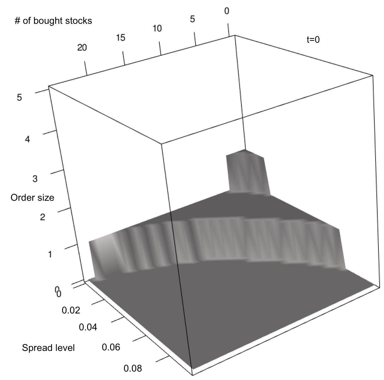
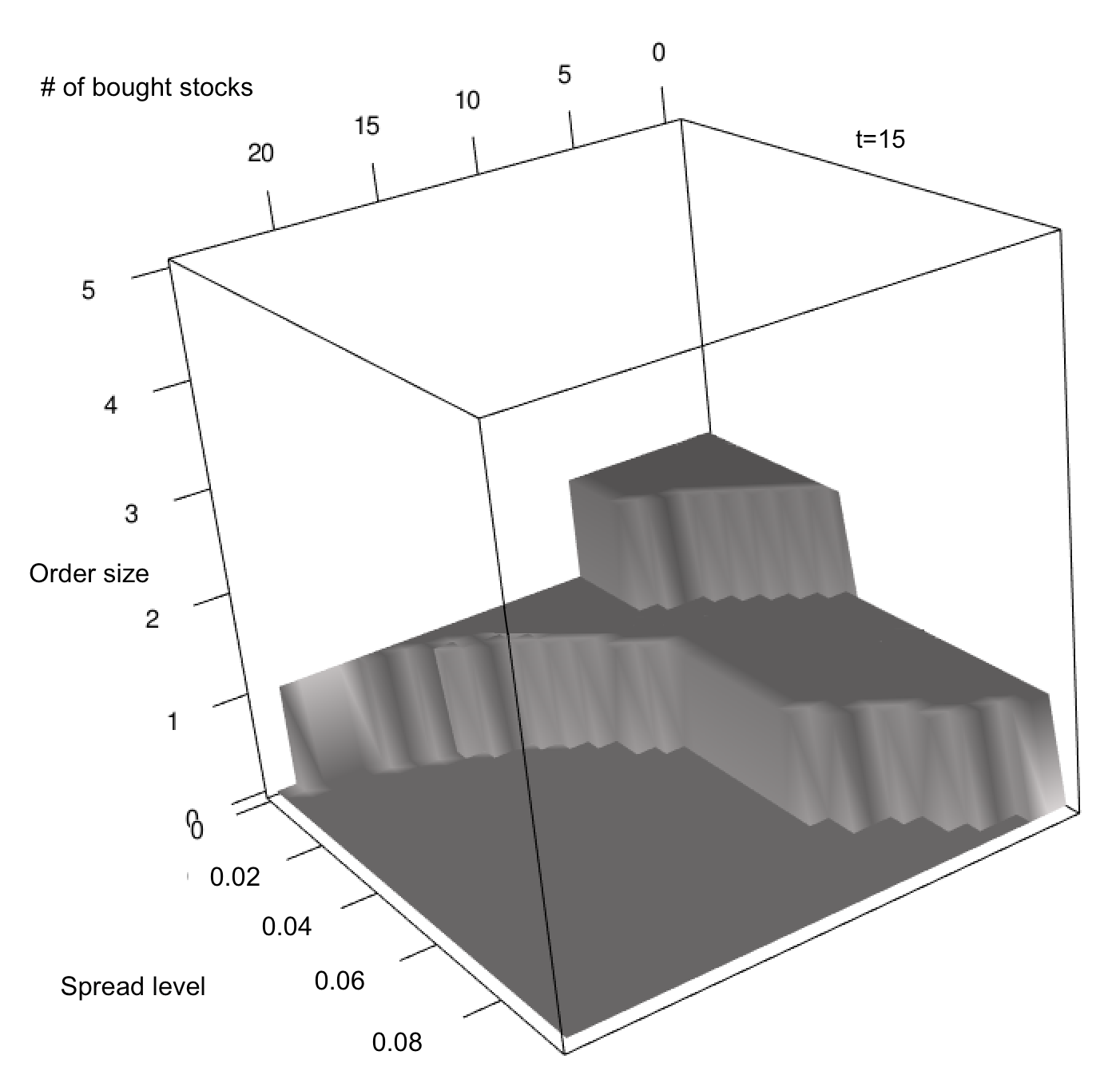
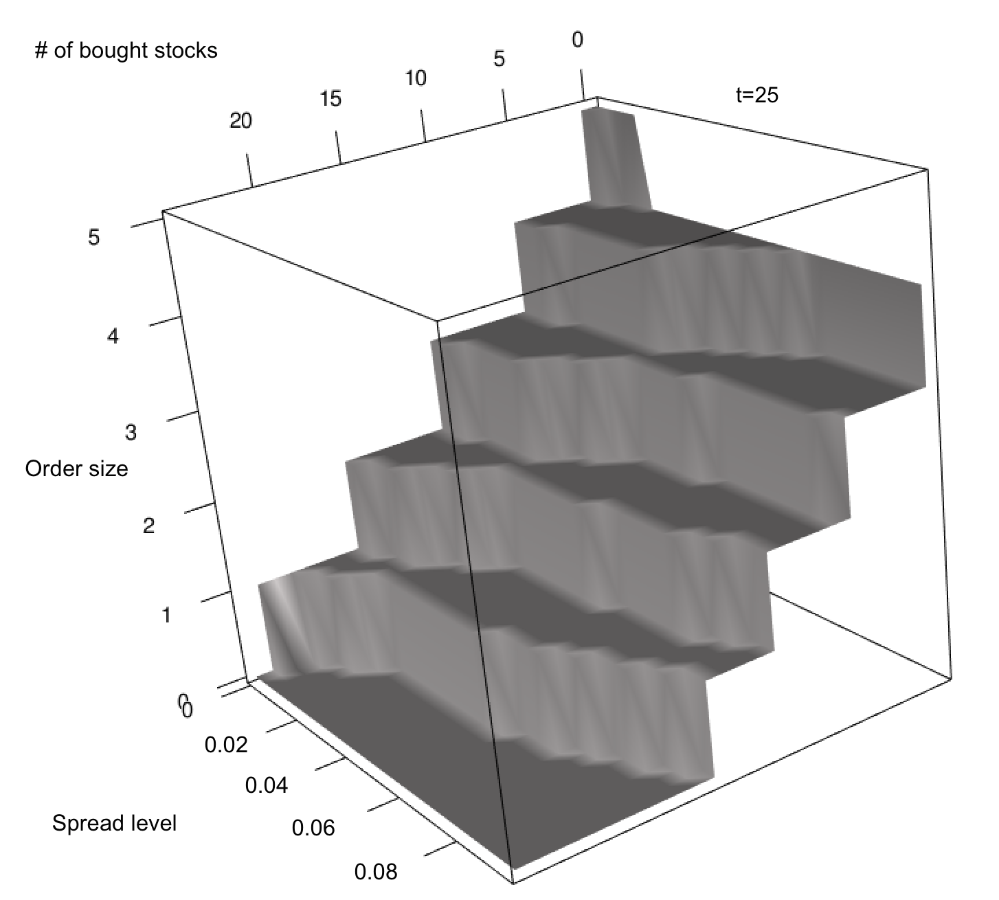
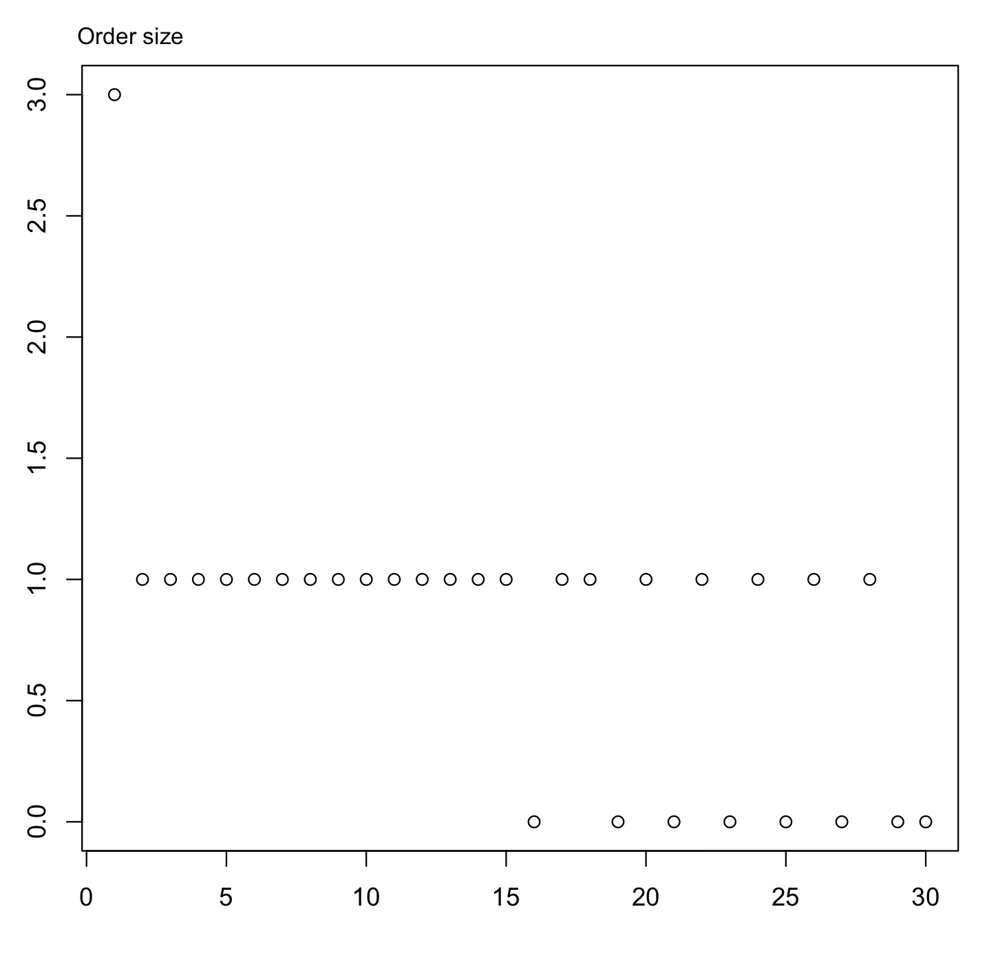
In Figure 1, we plot the optimal strategy for $\sigma_{\upsilon}(0)=5.10^{-4}$ and $m_{v}(0)=5.10^{-2}$ in terms of $(X^{2},X^{3})$. Clearly, the level of spread $X^{4}$ has a significant impact: when it is large, it is better to wait for it to decrease before sending a new order. This can also be observed in Figure 2 which provides a simulated path corresponding to an initial prior $(m_{v}(0)=2.10^{-2},\sigma_{\upsilon}(0)=10^{-3})$: after 15 seconds the algorithm alternates between sending an order and doing nothing, i.e. waiting for the spread to be reduced at the next time step. On the top right graph, we can also observe that the low mean of the initial prior combined with a zero initial resilience leads to sending an order of size 3 at first, then the mean of the prior is quickly adjusted to a higher level and the algorithm slows down immediately.

Figure 1: Evolution of $\beta$ in terms of $(X^{3},X^{4})$ at time $0$s (top), $15$s (left) and $25$s (right), for $(m_{\upsilon},\sigma_{\upsilon})=(5.10^{-2},5.10^{{-4}})$.

Figure 2: Evolution of $\beta$ (top left), price before (circles) and after (triangles) the impact (top right), $m_{\upsilon}$ (bottom left), $\sigma_{\upsilon}$ (bottom right), with time in second. The true value of $\upsilon$ is $5.10^{-2}$. $x$-axis: time in seconds.

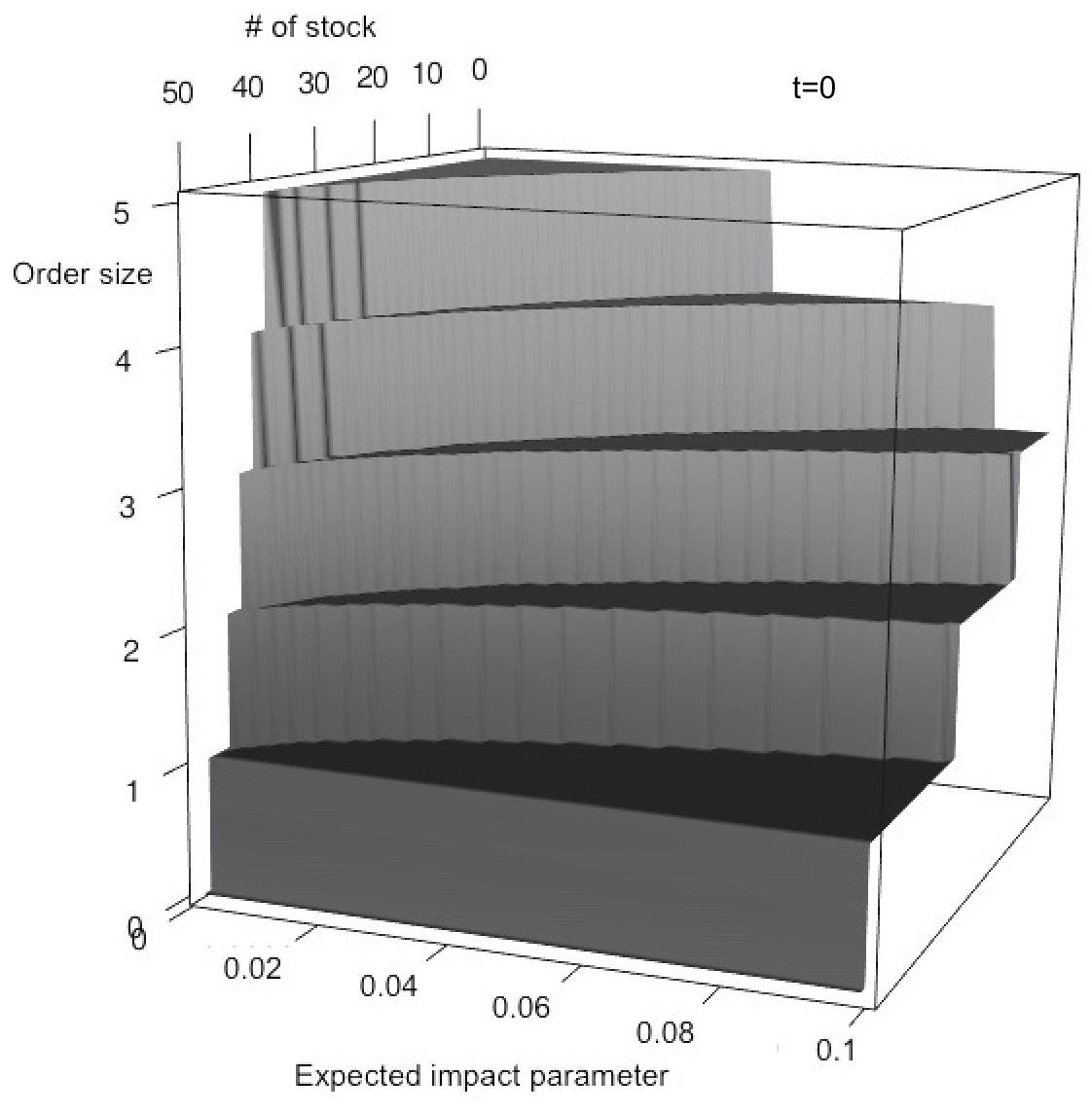
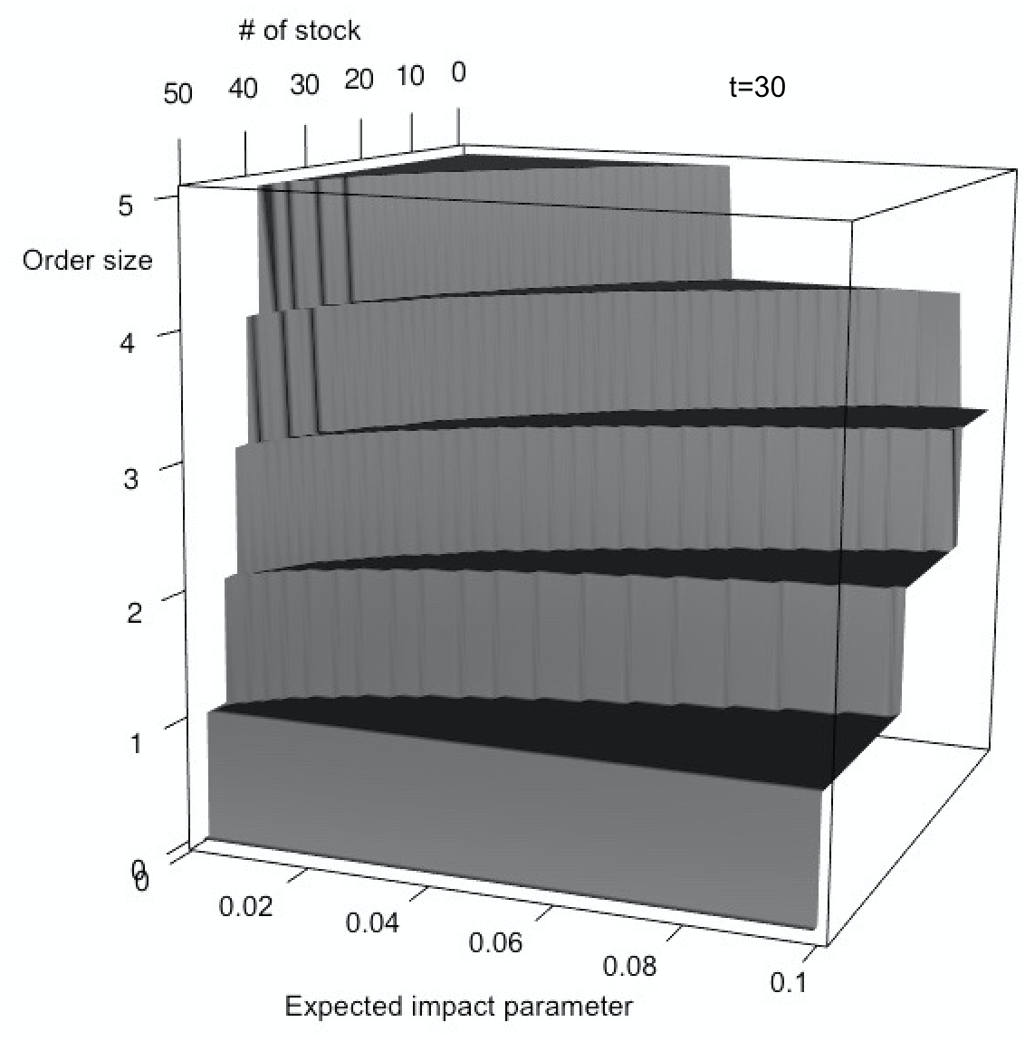
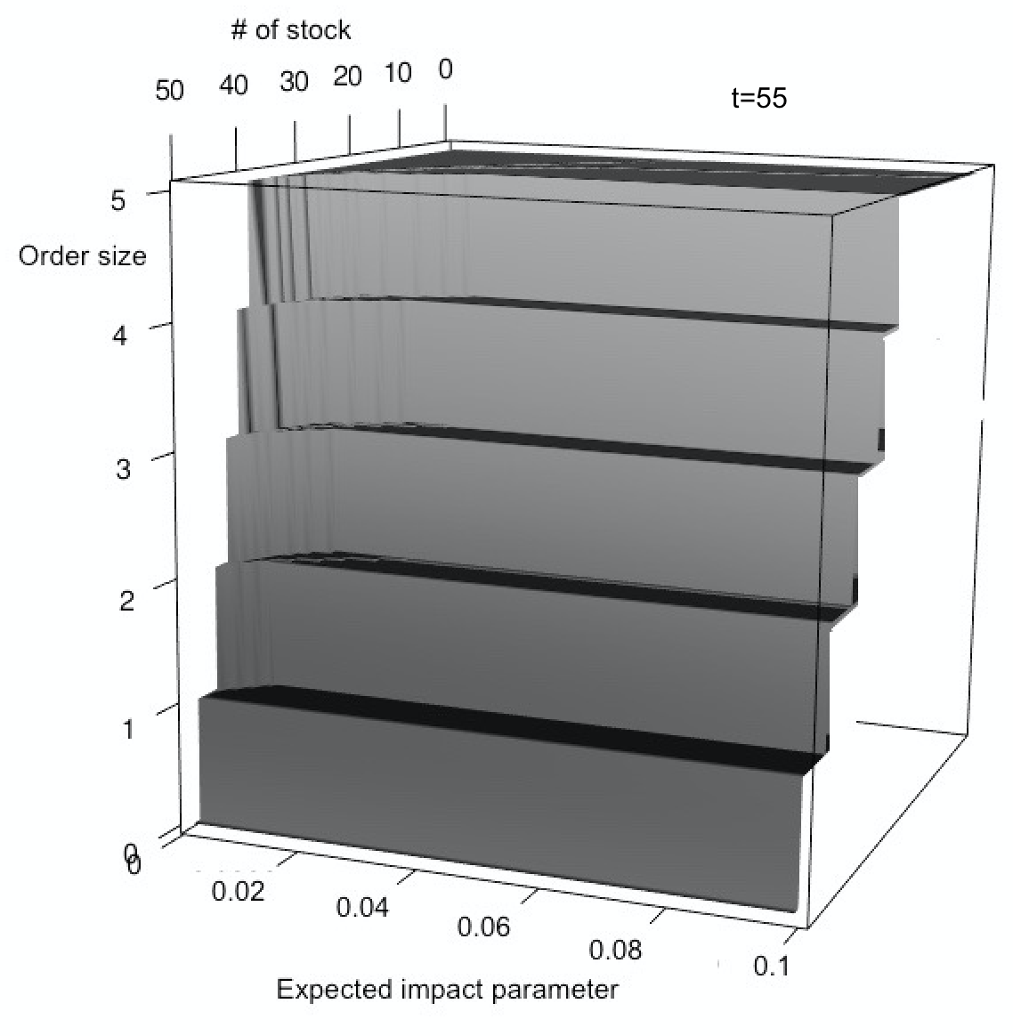
Let us now consider the case $\rho=0$, i.e. without dynamic resilience, with a trading period of $60$ seconds and $N=50$. In Figure 3, we provide the optimal policy (number of traded shares) in terms of the number $X^{3}$ of already traded shares and the prior’s mean parameter $m_{\upsilon}$ for different times. Not surprisingly the algorithm is more aggressive as the prior’s mean decreases and the remaining number of shares to buy increases. It is rather stable in time (compare $t=0$s with $t=30$s) up to the end where it is forced to accelerate to avoid a large final impact cost. It is also much more aggressive compared to the case $\rho>0$ presented above: we can no more make profit of the decrease of the resilience term $X^{4}$, and there is no reason to wait.

Figure 3: Evolution of $\alpha$ in terms of $(m_{\upsilon},X^{3})$ at time $0$s (top), $30$s (left) and $55$s (right), for $\sigma_{\upsilon}=5.10^{{-4}}$.

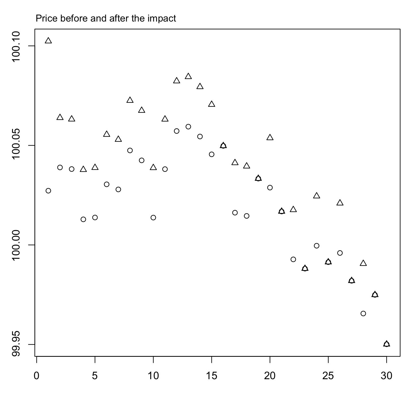
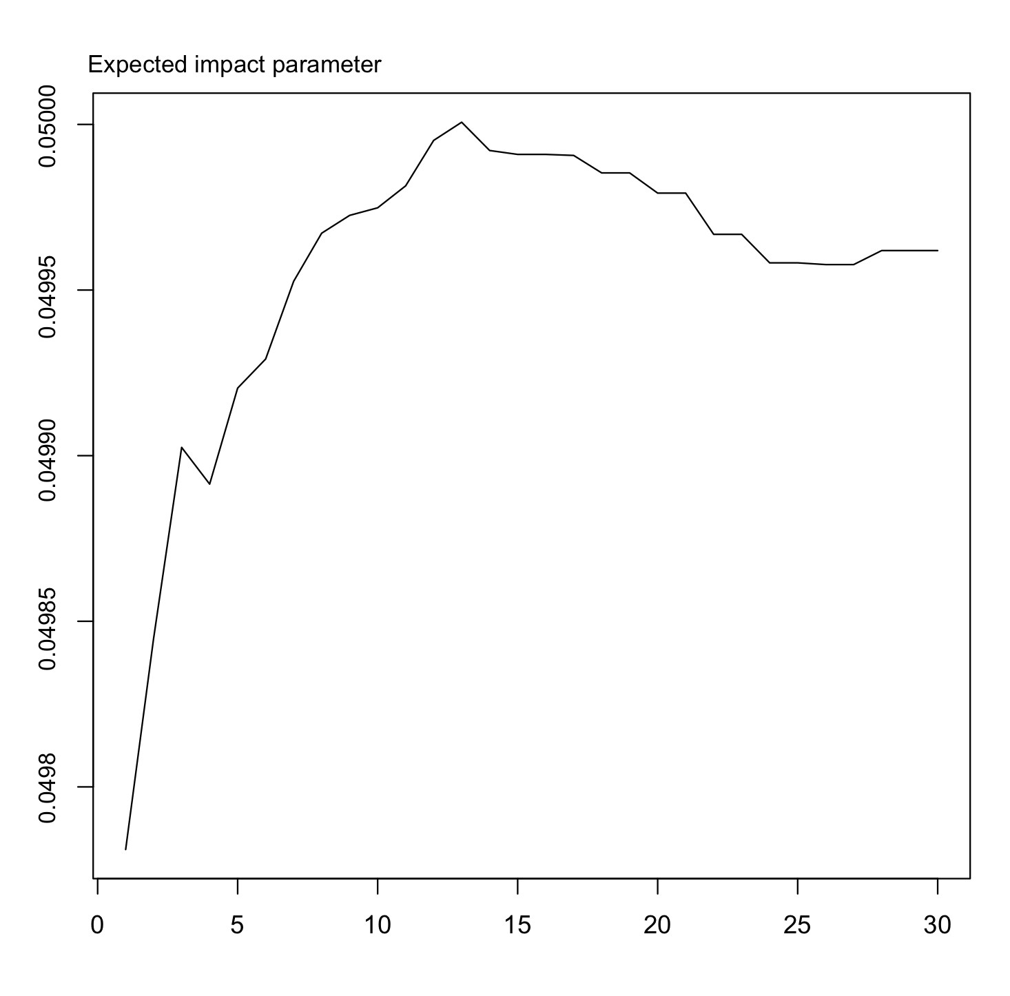
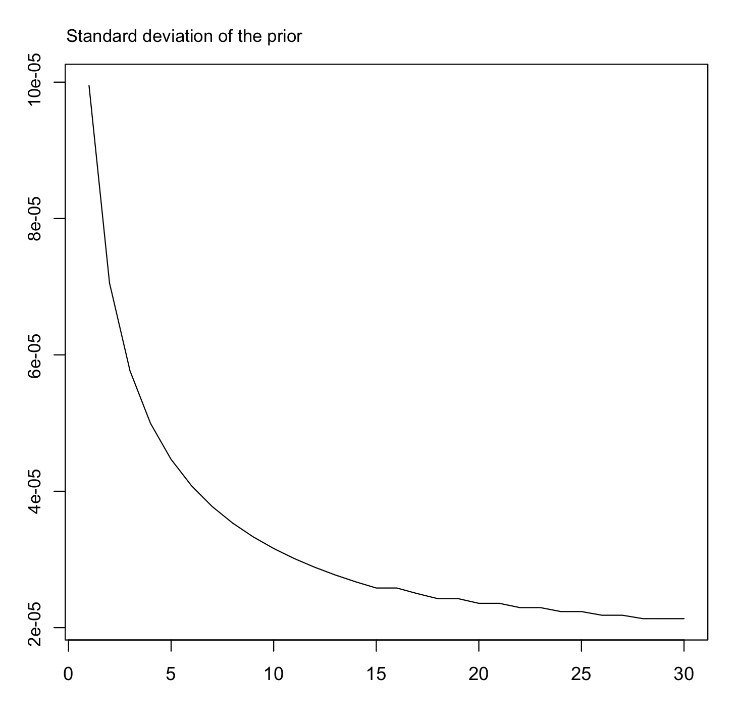
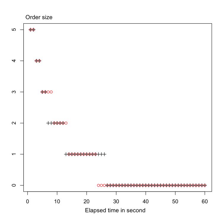
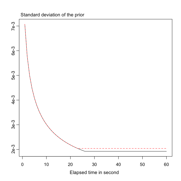
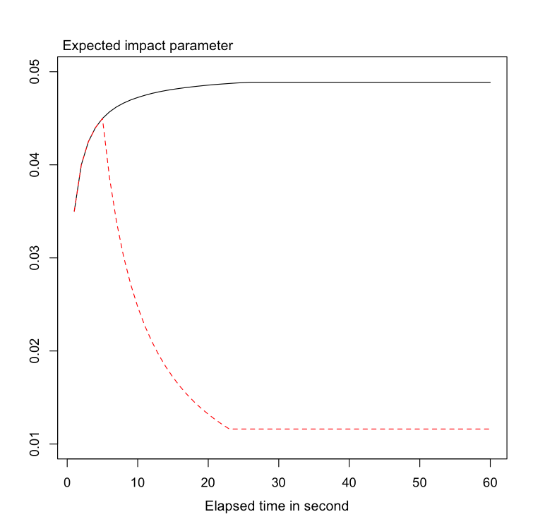
In Figure 4, we provide a simulated path of $(X,\alpha,m_{\upsilon},\sigma_{\upsilon})$ that shows how the prior on the unknown coefficients $\upsilon$ can adapt to changing market conditions. The red dashed lines and circles correspond to the same path of Brownian motion and the same realized noises $(\epsilon_{i})_{i\geq 1}$ as the black solid lines and crosses, but the true parameter is changed from $5.10^{-2}$ to $5.10^{-4}$ after $5$ seconds. It is more aggressive quite quickly after the shock as the prior adapts to the new small level of impact. Note that the total number of shares is bought slightly before $30$s, so that the prior do not change anymore after this date.

Figure 4: Evolution of $\alpha$ (top), $\sigma_{\upsilon}$ (left), $m_{\upsilon}$ (right) with time. Black crosses and black solid lines: the true value of $\upsilon$ is $5.10^{-2}$. Red circles and red dashed lines: the true value of $\upsilon$ is $5.10^{-2}$ for the first $5$ seconds, and then jumps to $5.10^{-4}$.

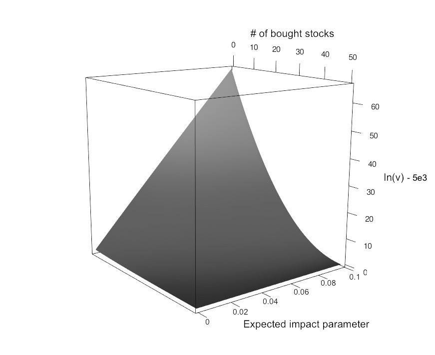
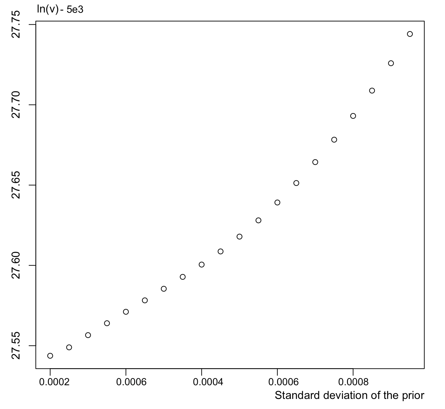
In Figure 5, we plot the log of the value function minus the cost $5.10^{3}$ of buying the total shares without impact (similar to the implementation shortfall), in terms of the different quantities of interest.

Figure 5: Top: $\ln({\rm v})-5.10^{3}$ in terms of $(x^{3},m_{\upsilon})$ for $\sigma_{\upsilon}=5.10^{-4}$ and $t=0$. Bottom: $\ln({\rm v})-5.10^{3}$ in terms of $\sigma_{\upsilon}$ for $(x^{3},m_{\upsilon})=(0,2.10^{-2})$ at $t=0$.

4.2 Random execution times: application to strategies using limit-orders

In this section, we consider a limit-order trading model. $X^{1}$ now represents a mid-price (of reference) and, between two trades, has the dynamic

$$dX_{t}^{1}=\sigma dW_{t}^{1}.$$ (4.2)

An order is of the form $(\ell,\beta)$ in which $\ell$ is the maximal time we are ready to wait before being executed, while $\beta$ is the price at which the limit order is sent. For simplicity, each order corresponds to buying one share.

We assume that the time $\theta$ it takes to be executed follows an exponential distribution of parameter $\rho(\upsilon,X_{\tau}^{1}-\beta)$, given the information at time $\tau$. One can send a new order only after $\vartheta:=\tau+\ell\wedge\theta$.

Hence, given a flow of orders $\phi=(\tau_{i},\ell_{i},\beta_{i})_{i\geq 1}$, the number $X^{3}$ of shares bought evolves according to

$$X^{3} =X_{\vartheta_{i}}^{3}\text{ \ on }[\vartheta_{i},\tau_{i+1})$$

$$X^{3}_{\vartheta_{i}} =X_{\tau_{i}-}^{3}+\mathbf{1}_{\left\{\theta_{i}\leq\ell_{i}\right\}},$$

in which $\vartheta_{i}:=\tau_{i}+\ell_{i}\wedge\theta_{i}$. Each $\theta_{i}$ follows an exponential distribution of parameter $\rho(\upsilon,X_{\tau_{i}}^{1}-\beta_{i})$ given ${\cal F}^{z,m,\phi}_{\tau_{i}-}$. As in the previous model, $X^{3}$ is restricted to $\{0,\ldots,N\}$. The total cost $X^{2}$ of buying the shares has the dynamics

$$X^{2} =X_{\vartheta_{i}}^{2}\text{ on }[\vartheta_{i},\tau_{i+1})$$

$$X^{2}_{\vartheta_{i}} =X_{\tau_{i}-}^{2}+\beta_{i}\mathbf{1}_{\left\{\theta_{i}\leq\ell_{i}\right\}}.$$

We want to maximize

$$-\mathbb{E}\left[e^{X^{2}_{{\rm T}[\phi]}+1.02(N-X^{3}_{{\rm T}[\phi]})+\frac{5.10^{2}}{2}(N-X^{3}_{{\rm T}[\phi]})^{2}}\wedge C\right],$$

in which $1.02$ is the best ask (kept constant) and $5.10^{2}$ is an impact coefficient. This corresponds to the cost of liquidating instantaneously the remaining shares $(N-x^{3})^{+}$ at $T$. This model is a version of [2], [16], [18], see also [17].

Direct computations show that the prior process $M$ evolves according to

$$M =M_{\vartheta_{i}}\text{ \ on }[\vartheta_{i},\tau_{i+1})$$

$$M_{\vartheta_{i}} =\mathfrak{M}_{1}(M_{\tau_{i}-};Z_{\vartheta_{i}},Z_{\tau_{i}-},\alpha_{i})\mathbf{1}_{\{\theta_{i}\leq\ell_{i}\}}+\mathfrak{M}_{2}(M_{\tau_{i}-};Z_{\vartheta_{i}},Z_{\tau_{i}-},\alpha_{i})\mathbf{1}_{\{\theta_{i}>\ell_{i}\}}$$

in which

$$\mathfrak{M}_{1}(m;t^{\prime},x^{\prime},t,x,l,b)[B]:=\frac{\int_{B}\rho(u,x^{1}-b)e^{-\rho(u,x^{1}-b)t^{\prime}}dm(u)}{\int_{\mathbb{R}^{+}}\rho(u,x^{1}-b)e^{-\rho(u,x^{1}-b)t^{\prime}}dm(u)}$$

and

$$\mathfrak{M}_{2}(m;t^{\prime},x^{\prime},t,x,l,b)[B]:=\frac{\int_{B}e^{-\rho(u,x^{1}-b)l}dm(u)}{\int_{\mathbb{R}^{+}}e^{-\rho(u,x^{1}-b)l}dm(u)}$$

for all Borel set $B$.

In the case where $\mathbf{M}$ is the convex hull of a finite number of Dirac masses, then the weights associated to $M$ can be computed explicitly.

Here again, the map $\Psi(t,x,m)=N-x^{3}$ satisfies the conditions provided in [4] to ensure that Assumption 3.1 holds.

We now consider a numerical illustration. We take $C=10^{200}$. The time horizon is $T=15$ minutes. To simplify, we fix the reference mid-price to be $X^{1}\equiv 1$ (i.e. $\sigma=0$) and restrict to $\ell=1$, i.e. an order is sent each minute. We take $N=10$. One can send limit buy orders in the range $B:=\{0.90,0.92,0.94,0.96,0.98\}$.

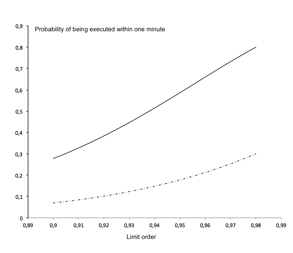
As for the intensity of the execution time, we use an exponential form as in [16]: $\rho(u,x^{1}-b)=\lambda(u)e^{-20(0.98-b)}$ in which $\lambda(u)=-\ln(1-u)$. This means that the probability to be executed at the price 0.98 within one minute is $u$. Orders are sent each minute, but we use a finner time grid in order to take into account that it can be executed before this maximal time-length. The original prior is supported by two Dirac masses at $u=0.3$ and $u=0.8$. The corresponding probabilities of being executed within one minute are plotted in Figure 6.

Figure 6: Solid: $u=0.8$. Dashed: $u=0.3$

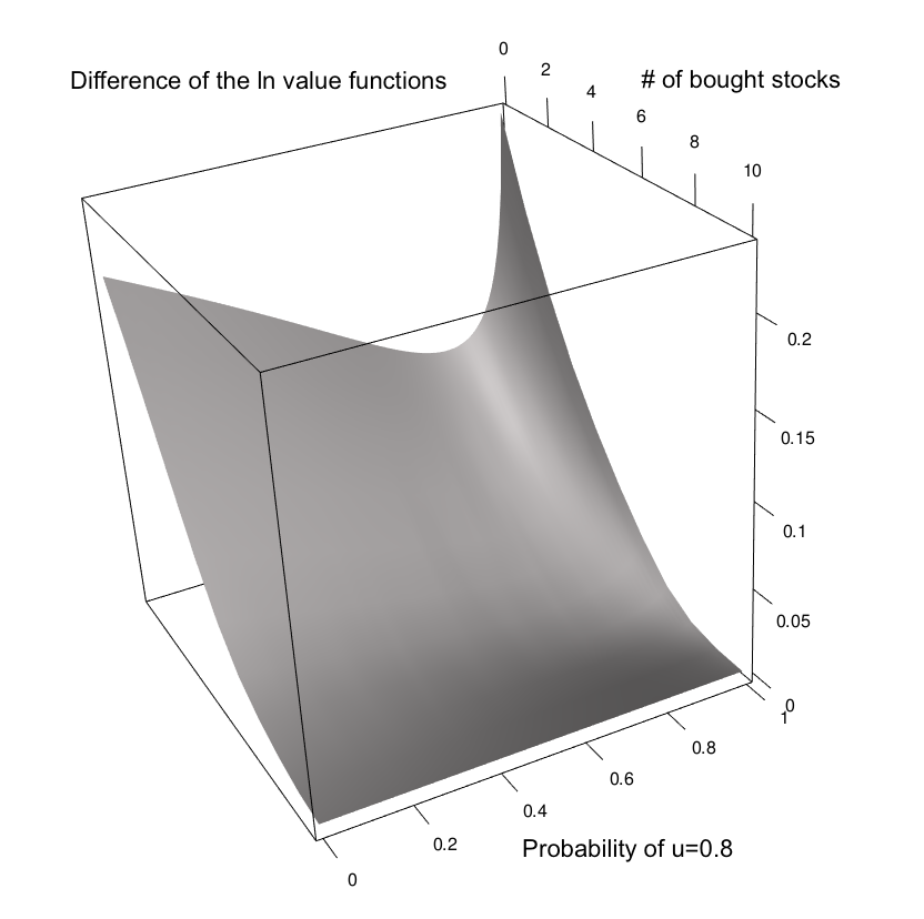
Our time step corresponds to 15 seconds, so that every 15 seconds the controller can launch a new order if the previous one has been executed before the maximal 1 minute time-length. In Figure 7, we plot the difference, in logarithms, between the value functions obtained in the latter case and for a time step of 1 minute (in which case a new order cannot be launched before one minute). Clearly, the possibility of launching new orders in advance is an advantage.

Figure 7:

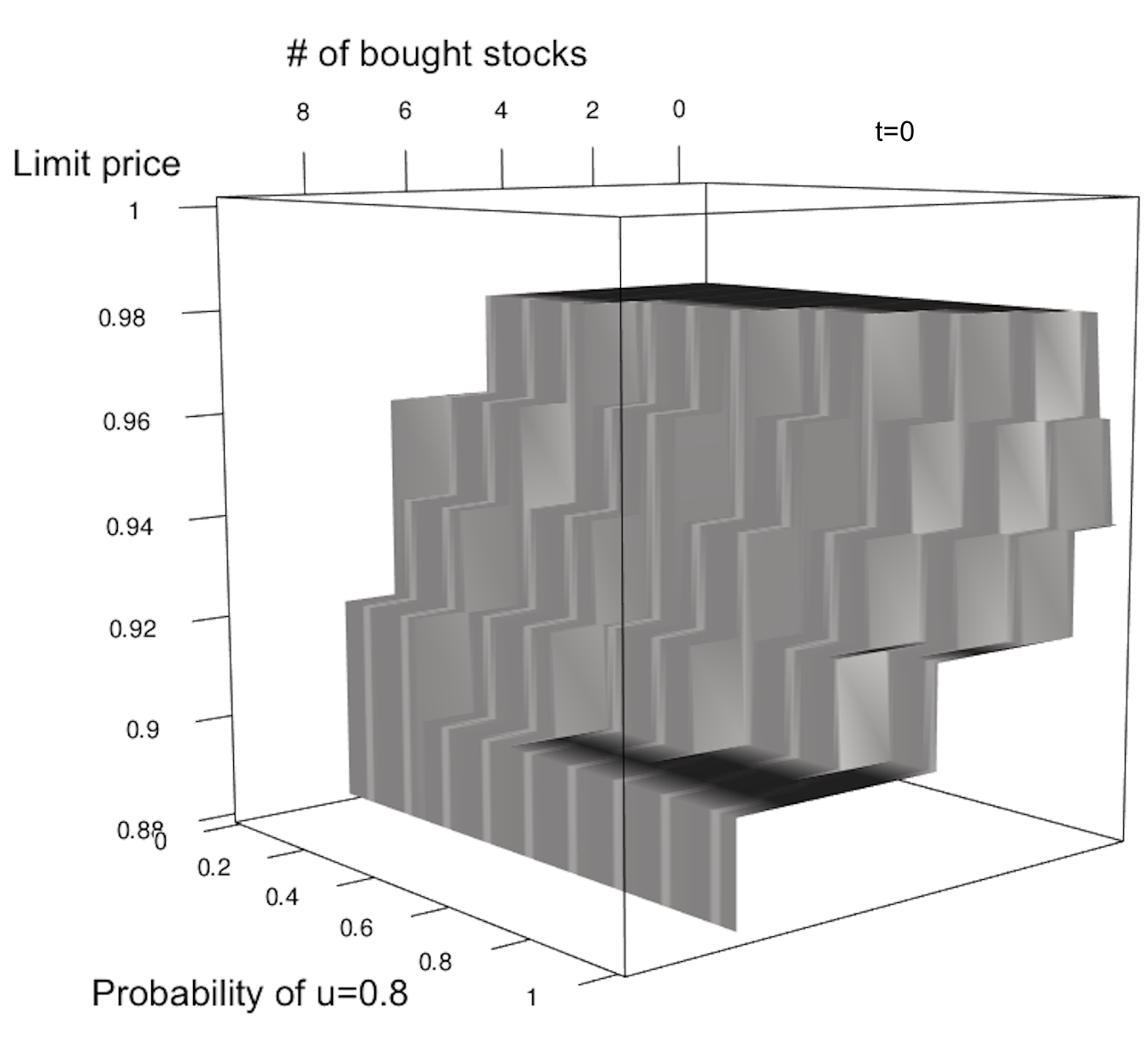
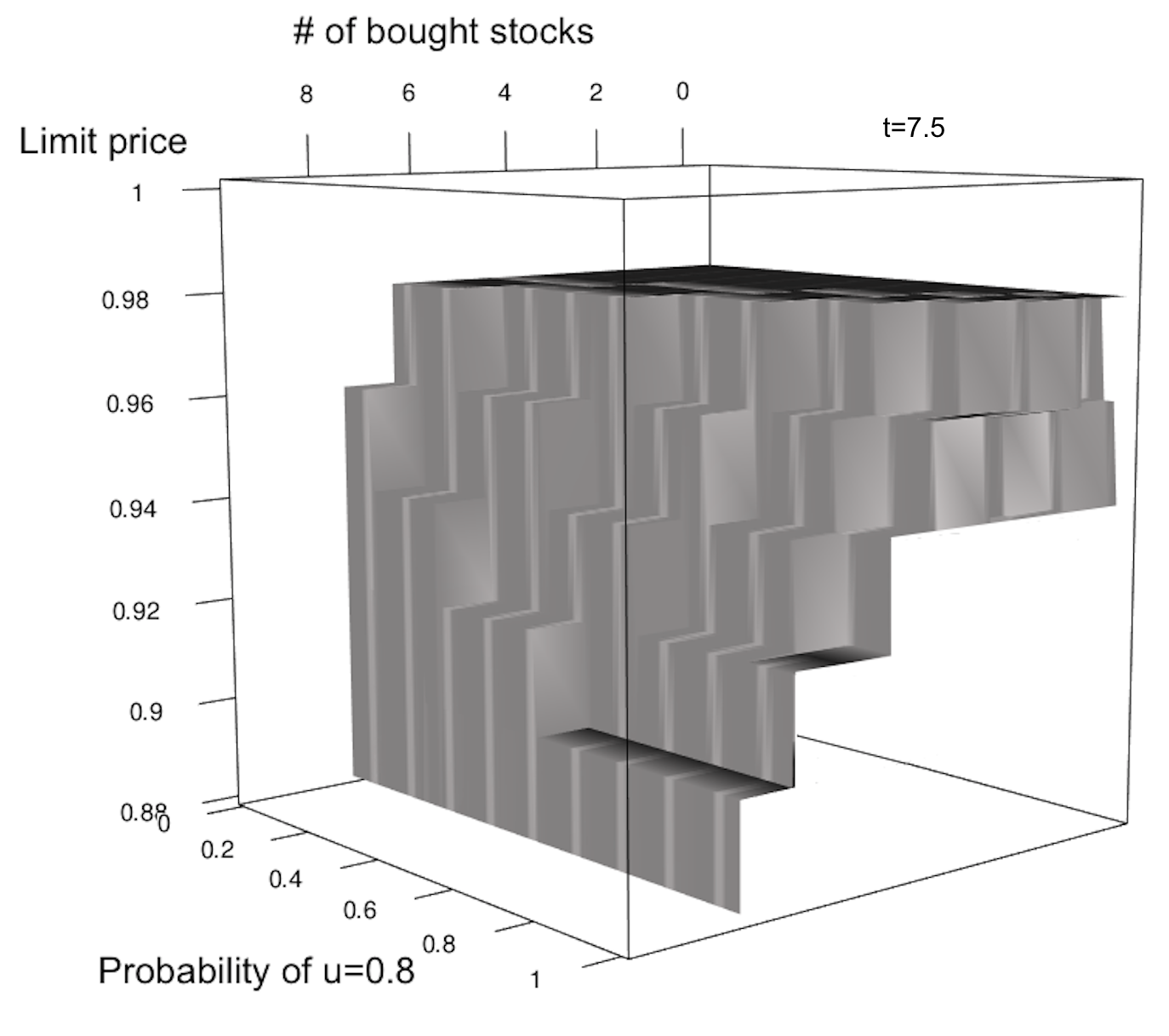
In Figure 8, we plot the optimal policy at time $t=0$ and $t=7.5$ minutes. As expected, the algorithm is more aggressive when the probability of having $\upsilon=0.8$ is higher.

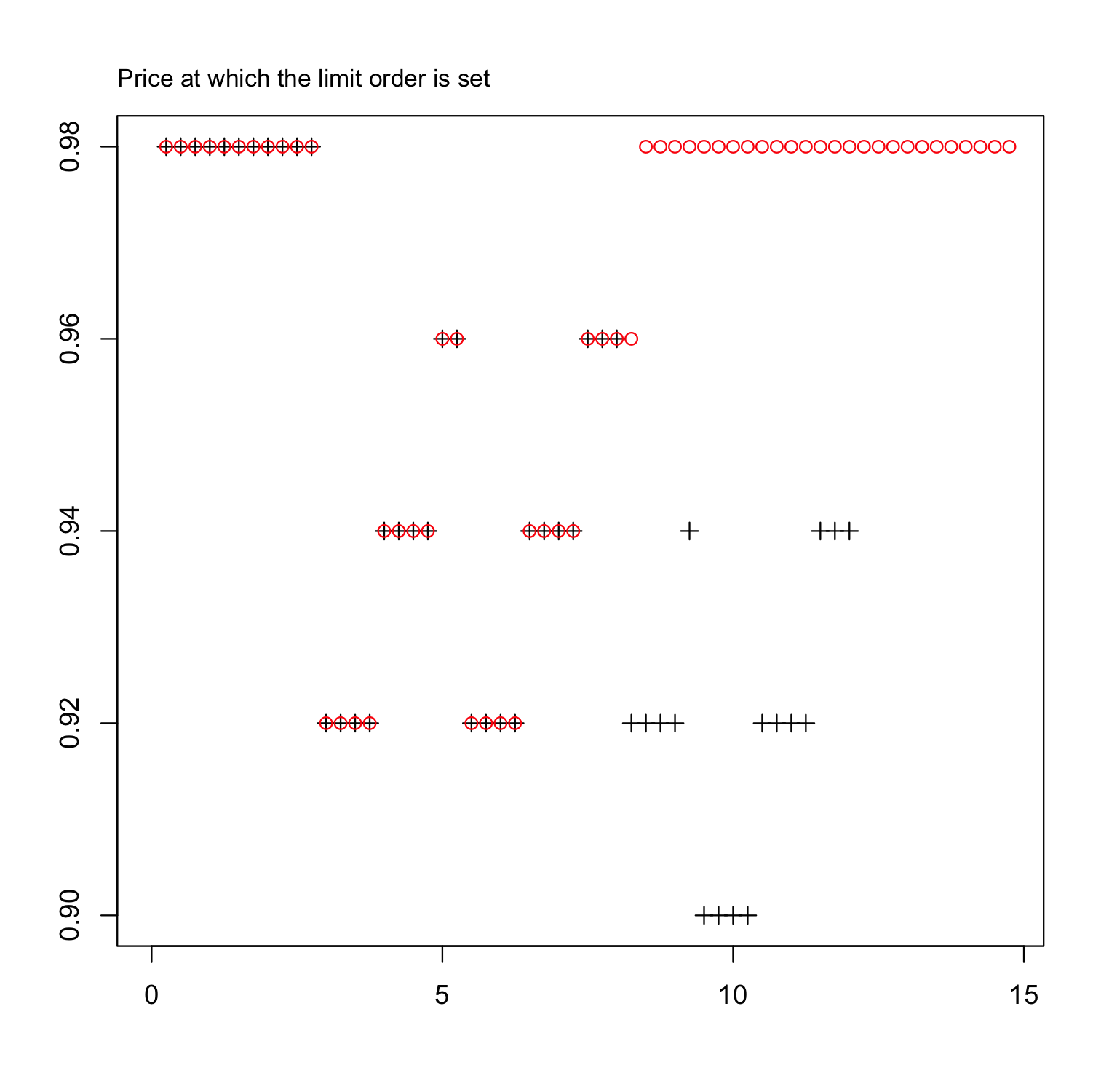
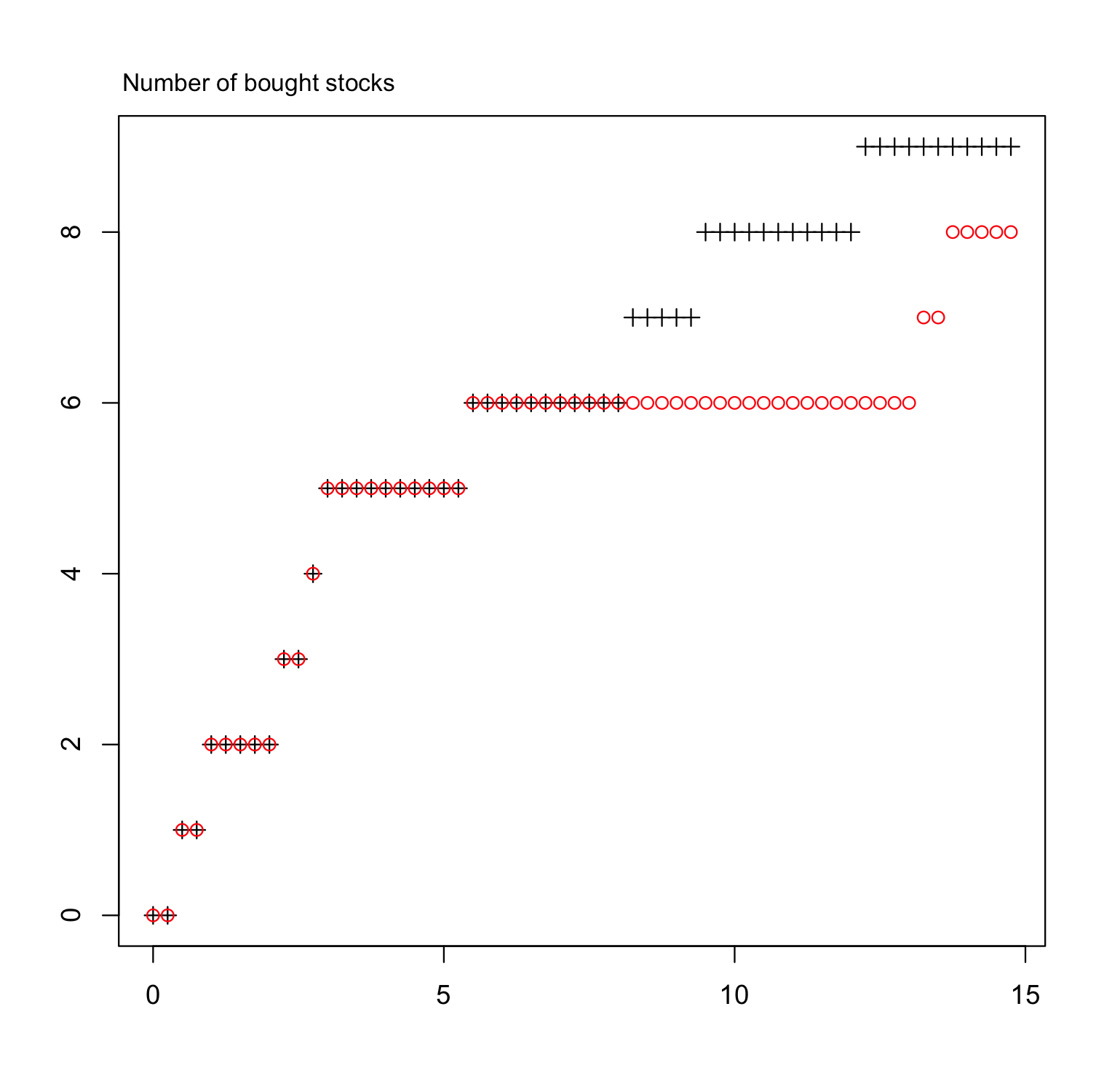
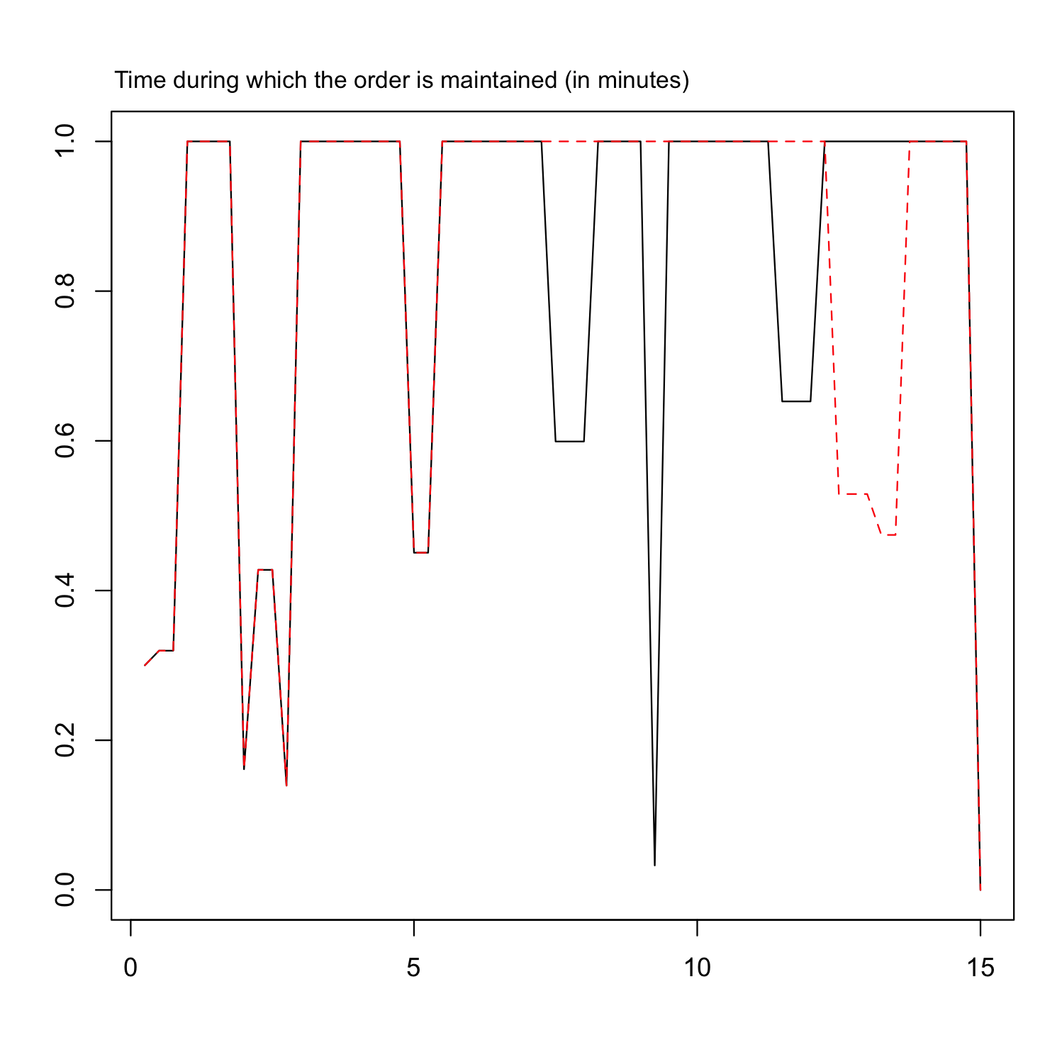
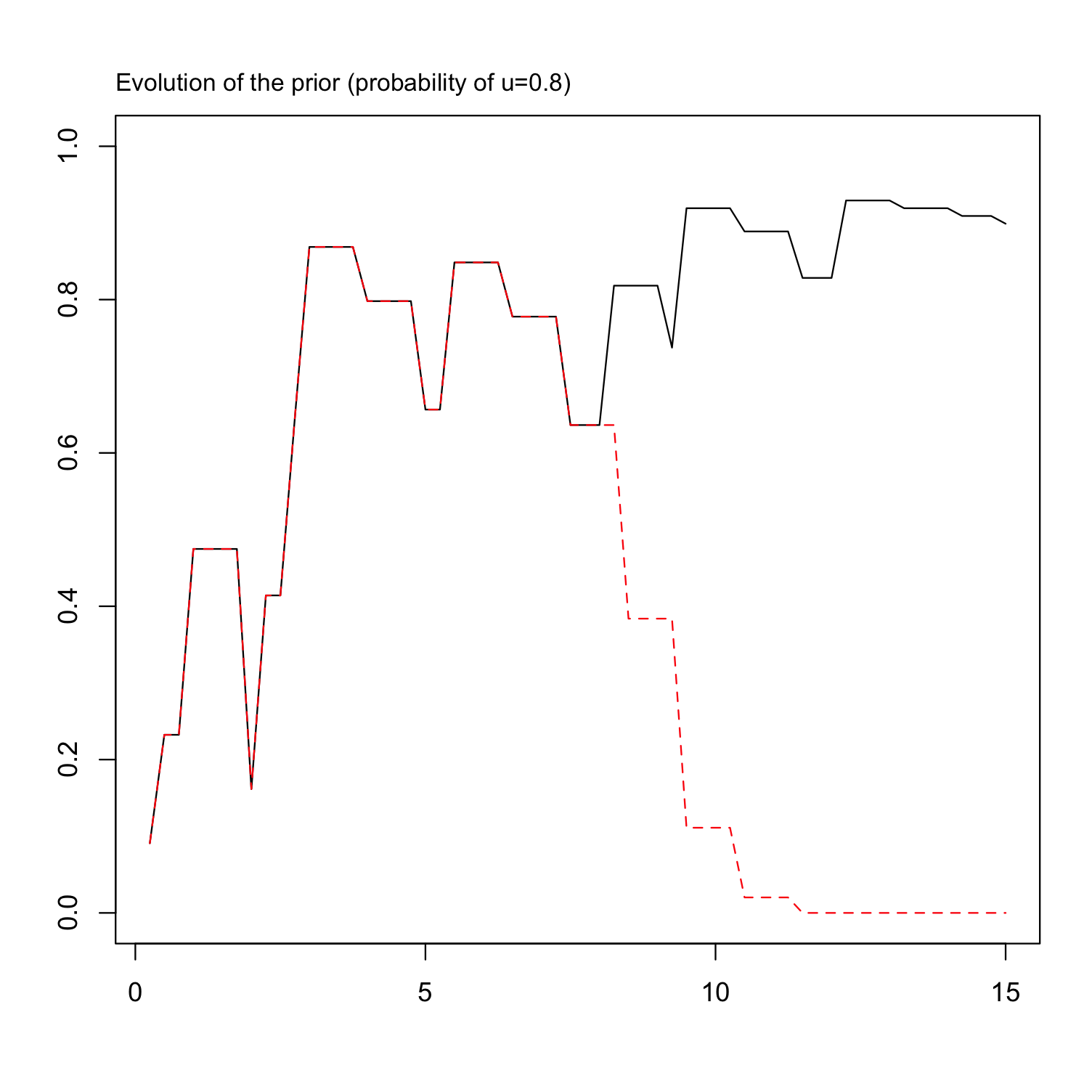
In Figure 9, we plot a simulated path. The red and black lines and points correspond to the same realization of the random variables at hand, but for different values of the real value of $\upsilon$. Black corresponds to the most favorable case $\upsilon=0.8$, while red corresponds to $\upsilon=0.8$ for the first $7.5$ minutes and $\upsilon=0.3$ for the remaining time. The initial prior is $\mathbb{P}[\upsilon=0.8]=9\%$. Again, the algorithm adapts pretty well to this shock on the true parameter. We also see that it is more aggressive when the prior probability of being in the favorable case is high.

Figure 8: Top: $t=0$. Bottom: $t=7.5$ minutes

Figure 9: Black crosses and solid lines: $\upsilon=0.8$. Red circles and dashed lines: $\upsilon=0.8$ before $t=7.5$ minutes and $\upsilon=0.3$ after. $x$-axis$=$ time in minutes.

.

References

- [1] R. Almgren and J. Lorenz. Bayesian adaptive trading with a daily cycle. The Journal of Trading, 1(4):38–46, 2006.
- [2] M. Avellaneda and S. Stoikov. High-frequency trading in a limit order book. Quantitative Finance, 8(3):217–224, 2008.
- [3] E. Bacry and J.-F. Muzy. Hawkes model for price and trades high-frequency dynamics. Quantitative Finance, 14(7):1147–1166, 2014.
- [4] N. Baradel, B. Bouchard, and N.-M. Dang. Optimal control under uncertainty and bayesian parameters adjustments. Hal preprint, 2016.
- [5] G. Barles. An introduction to the theory of viscosity solutions for first-order hamilton–jacobi equations and applications. In Hamilton-Jacobi equations: approximations, numerical analysis and applications, pages 49–109. Springer, 2013.
- [6] G. Barles and P.E. Souganidis. Convergence of approximation schemes for fully nonlinear second order equations. In Decision and Control, 1990., Proceedings of the 29th IEEE Conference on. IEEE, 1990.
- [7] A. Bensoussan. Stochastic control of partially observable systems. Cambridge University Press, 2004.
- [8] B. Bouchard, M. Dang, and C.-A. Lehalle. Optimal control of trading algorithms: A general impulse control approach. SIAM Journal on financial mathematics, 4:404–438, 2011.
- [9] J.-P. Bouchaud. Price impact. Encyclopedia of quantitative finance, 2010.
- [10] X. Brokmann, E. Sérié, J. Kockelkoren, and J.-P. Bouchaud. Slow decay of impact in equity markets. arXiv preprint arXiv:1407.3390, 2014.
- [11] F. Camilli and M. Falcone. An approximation scheme for the optimal control of diffusion processes. Modélisation mathématique et analyse numérique, 29(1):97–122, 1995.
- [12] F. Camilli and E. R. Jakobsen. A finite element like scheme for integro-partial differential hamilton-jacobi-bellman equations. SIAM Journal on Numerical Analysis, 47(4):2407–2431, 2009.
- [13] S. Delattre, C. Y. Robert, and M. Rosenbaum. Estimating the efficient price from the order flow: a brownian cox process approach. Stochastic Processes and their Applications, 123(7):2603–2619, 2013.
- [14] T. E. Duncan and B. Pasik-Duncan. Adaptive control of continuous time stochastic systems. International Journal of Adaptive Control and Signal Processing, 16(5):327–340, 2002.
- [15] D. Easley and N. M. Kiefer. Controlling a stochastic process with unknown parameters. Econometrica: Journal of the Econometric Society, pages 1045–1064, 1988.
- [16] O. Guéant, C.-A. Lehalle, and J. Fernandez-Tapia. Optimal portfolio liquidation with limit orders. SIAM Journal on Financial Mathematics, 3(1):740–764, 2012.
- [17] O. Guéant, C.-A. Lehalle, and J. Fernandez-Tapia. Dealing with the inventory risk: a solution to the market making problem. Mathematics and financial economics, 7(4):477–507, 2013.
- [18] T. Ho and H. R. Stoll. Optimal dealer pricing under transactions and return uncertainty. Journal of Financial economics, 9(1):47–73, 1981.
- [19] S. Laruelle, C.-A. Lehalle, and G. Pagès. Optimal split of orders across liquidity pools: a stochastic algorithm approach. SIAM Journal on Financial Mathematics, 2(1):1042–1076, 2011.
- [20] S. Laruelle, C.-A. Lehalle, and G. Pagès. Optimal posting price of limit orders: learning by trading. Mathematics and Financial Economics, 7(3):359–403, 2013.
- [21] C.-A. Lehalle and S. Laruelle. Market microstructure in practice. World Scientific Publishing Co. Pte. Ltd., 2013.
- [22] M. Rosenbaum. Étude de quelques problèmes d’estimation statistique en finance. PhD thesis, ENSAE ParisTech; Université Paris-Est, 2007.