Markov models for ocular fixation locations in the presence and absence of colour

Abstract

We propose to model the fixation locations of the human eye when observing a still image by a Markovian point process in $\mathbb{R}^{2}$. Our approach is data driven using k-means clustering of the fixation locations to identify distinct salient regions of the image, which in turn correspond to the states of our Markov chain. Bayes factors are computed as model selection criterion to determine the number of clusters. Furthermore, we demonstrate that the behaviour of the human eye differs from this model when colour information is removed from the given image.

1 Introduction

Ocular movement data has posed a particularly tough challenge to researchers and offers many potential insights into human visual behaviour as well as many practical applications. The contribution, if any, of colour information to vision through saliency models and fixation location prediction has been heavily investigated; see Baddeley and Tatler (2006), Frey et al. (2008), Ho-Phuoc et al. (2012), Hamel et al. (2014). Much research has gone into understanding ocular movement from the rapidly jerking saccades to the relatively still fixations. In this article, we will specifically focus on the eye’s fixations by modelling such a sequence of fixations as a point process in $\mathbb{R}^{2}$. The distribution of fixations over a given image is treated as a finite mixture model comprised of disjoint salient regions, which correspond to the interesting bits of the image; see McLachlan and Peel (2004). This set of salient regions is used as the state space of a Markov chain. Each fixation is then an observation from the mixture component corresponding to the current state of the Markov chain. Under this model, it is shown that the presence or absence of colour information in the image drastically effects the behaviour of a given sequence of fixations.

The data under scrutiny comes for the study of Ho-Phuoc et al. (2012) who were interested as to whether the presence, absence, or modification of the colour of a photograph affects how the eye moves when looking at a given image. There were three colour schemes in their study: normal colours; abnormal colours; and grayscale. Normal refers to the unmodified image. Abnormal corresponds to swapping the red-green and blue-yellow chrominance channels. Grayscale corresponds to the complete removal of all colour information. An example of the three colour schemes with plotted fixations is displayed in Figure 1.

Figure 1: An example of the three colour schemes, normal, abnormal, and grayscale, respectively, under analysis with plotted fixations.

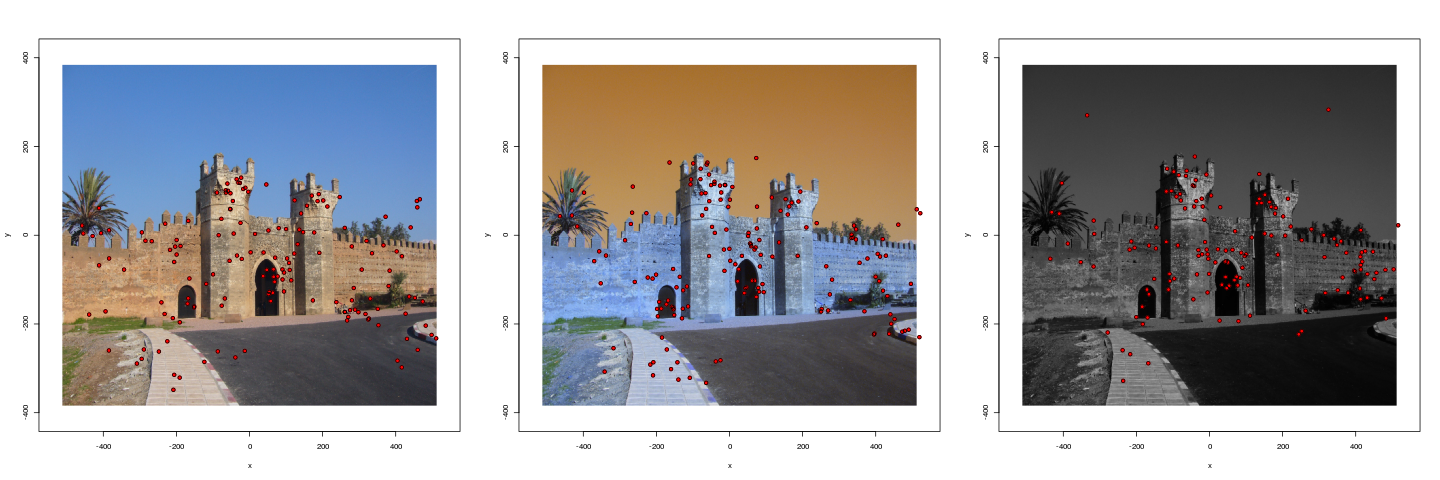
The data was collected as follows. Ten observers were selected for each of the three colour schemes totaling 30 subjects in all. Each subject was presented with 60 photographs under a fixed colour scheme. Each photo was displayed for five seconds, and the position and duration of each fixation was recorded. An example of ten rows sampled from the data set are displayed in Table 1 whose entries from left to right are horizontal and vertical position of the fixation, the duration in milliseconds, the fixation’s sequence number, the subject identifier, the colour scheme, the image number, and the orientation of the image. A more detailed explanation of the data, the experiment, and the method of collection can be found in Ho-Phuoc et al. (2012).

Statistical analysis of static spatial point patterns and spatial point processes has been used in this context; for an overview; see Diggle (2003), Illian et al. (2008). Modeling eye fixations as a spatial point process was previously discussed in Barthelmé et al. (2013) where an inhomogeneous Poison process (IPP) was utilized. The location dependent rate parameter of the IPP was determined by a measure of the saliency of each region of a given photograph. Alternatively, Kümmerer et al. (2014) apply deep neural networks in order to identify salient regions and ultimately to predict fixations. But as is mentioned in Ho-Phuoc et al. (2012), “there is no computational saliency model that can predict an observer’s fixation location better than the model using fixations from other subjects.” In light of that, we take a data driven approach to modelling sequential fixation locations using nine of the ten subjects to train our model and the tenth for validation. Bayes factors are used as a model selection criterion; see Good (1967) for the use of Bayes factors in the multinomial hypothesis setting, and Kass and Raftery (1995) for a general overview of Bayes factors and model selection. With additional thought, our Markov states could ultimately be constructed from a saliency map of the image itself rather than from the data.

In this article, Section 2 introduces a discrete time Markov model for the observed sequences of ocular fixations. The states are determined through $k$-means clustering where cross validation is used to determine the optimal number of clusters. A further investigation of alternative clustering methods, a post-hoc look at the Markov transition probabilities, a closer analysis of saccade lengths, and a display of the best and worst scoring photographs under our model can be found in Sections 2.1, 2.2, 2.3, and 2.4, respectively. Section 3 discusses various potential extensions to this model. This includes Section 3.1, which proposes reworking the discrete model as a continuous time Markov process through a closer analysis of the fixations’ durations, and Section 3.2, which discusses a saliency driven approach to model construction in contrast to our data driven method. Lastly, Section 4 concludes with potential applications.

Table 1: Ten randomly sampled entries from the data set.

$X$ $Y$ Time Fix. Subj. Colour Image Format 80. 4 74. 8 980 10 a5 abnormal 53 landscape -213. 4 111. 6 246 6 n5 normal 48 landscape 499. 9 151. 8 241 10 a5 abnormal 11 landscape -32. 7 146. 3 150 5 a3 abnormal 51 landscape -256. 3 183. 6 135 10 n3 normal 4 landscape 112. 6 86. 0 276 12 g7 grayscale 47 landscape 214. 5 -133. 9 295 10 a4 abnormal 59 landscape 409. 3 0. 8 225 12 a9 abnormal 30 landscape 226. 4 -343. 8 413 3 g2 grayscale 44 landscape -111. 0 -115. 2 157 8 a10 abnormal 25 landscape

2 Discrete time Markov model

Figure 2: The four clusters of fixation locations for a given image, and the corresponding kernel density estimates for the fixation location model.

Consider a sequence of fixation positions $X_{1},\ldots,X_{n}\in\mathbb{R}^{2}$ as a point process in $\mathbb{R}^{2}$ and an associated sequence of states $S_{1},\ldots,S_{n}\in\{1,\ldots,k\}$. We will model this state sequence as a Markov chain jumping between $k$ different clusters corresponding to interesting parts of the photo. The fixation sequence will then be random observations conditioned on the current state of the Markov chain. The model selection will decide between such models for $k=1,\ldots,10$. The $k=1$ case, our null model with which to compare the others, is the naive model that the $X_{t}$ are independent and identically distributed draws from some underlying density $f(x)$. For $k\geq 2$, we suppose a finite mixture model with $k$ constituent densities $f_{1},\ldots,f_{k}$ corresponding to on which part of the image the eye is focusing. In this model, the states evolve via a Markov chain with $X_{t}$ given by an independent random draw from $f_{S_{t}}(x)$.

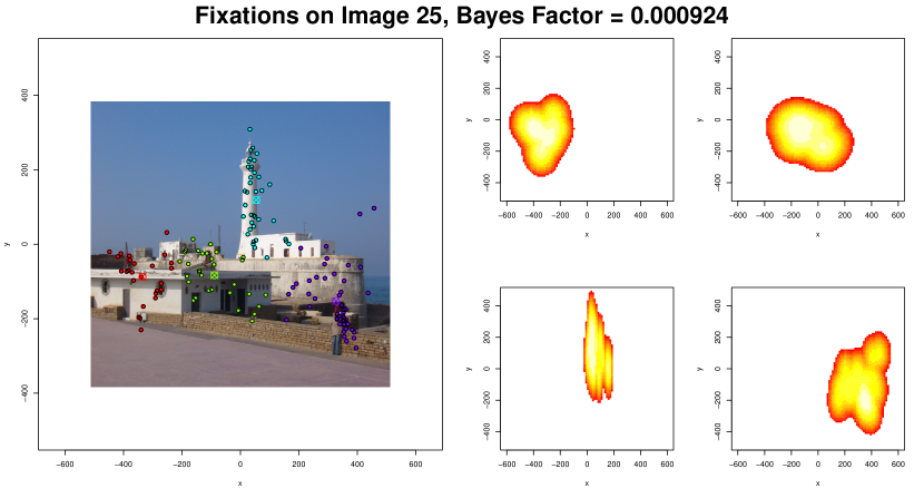
These constituent densities were modelled empirically by clustering the fixation locations from nine of the ten subjects; the model was then tested on the tenth. Cross-validation was performed across all training subjects to optimise this model. Let $X_{1},\ldots,X_{n}$ be the test sequence of fixation locations and $Y_{t}^{(j)}$ be fixation $t$ of subject $j$ from the training set. A Bayes factor was computed for each subject, and the results were averaged into a final score for each picture. The training fixation points were clustered via $k$-means clustering with 10 random starts. Other clustering methods are discussed in Section 2.1. For each cluster, a two dimensional kernel density estimate with Gaussian kernel was computed. An example of these clusters and density estimates can be seen in Figure 2. Each fixation in the test set was assigned a cluster based on proximity to the cluster center. A $k$-nearest neighbours classifier was also implemented to assign clusters, but returned very similar results.

The observed initial states and transitions between states were treated as observations from a multinomial random variable with a Dirichlet conjugate prior. Specifically, the Markov initial, $\pi$, and transition probabilities, $p$, were treated as Dirichlet random variables with the Jeffreys prior and updated by the nine subjects in the training data. Let $c_{i}$ be the number of initial fixations $Y_{1}^{(j)}$ in state $i$, and let $m_{i,i^{\prime}}$ be the number of observed transitions from $Y_{t-1}^{(j)}\in S_{i}$ to $Y_{t}^{(j)}\in S_{i^{\prime}}$. The posteriors are

$$\pi \sim\text{Dirichlet}\left(0.5+c_{1},\ldots,0.5+c_{k}\right),$$

$$p_{i,\cdot} \sim\text{Dirichlet}\left(0.5+m_{i,1},\ldots,0.5+m_{i,k}\right).$$

Therefore, the Bayes factor is

$$BF=\frac{\mathrm{P}\left(X_{t}\,\middle|\,Y_{t},k=1\right)}{\mathrm{P}\left(X_{t}\,\middle|\,Y_{t},k\right)}=\frac{\prod_{t=1}^{n}f(X_{t})}{\mathrm{E}_{\pi,p}\left\{\pi_{s_{1}}f_{s_{1}}(X_{1})\prod_{t=2}^{n}p_{s_{t-1},s_{t}}f_{s_{t}}(X_{t})\right\}}$$

where the expectation is taken with respect to the Dirichlet posterior. In practice, this value is approximated via Monte Carlo integration.

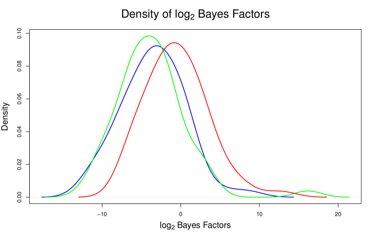
A plot depicting a kernel density estimates for the $\log_{2}$ Bayes factors of each colour scheme is displayed in Figure 3. The red curve corresponding to the density of the grayscale Bayes factors appears shifted further to the right than the other two. Indeed, performing three paired t-tests results in the following 95% confidence intervals and p-values:

Norm - Abno: $$[-1.25,\phantom{-}1.71] p =0.76,$$ -value

Norm - Gray: $$[-4.26,-1.77] p =9.6\times 10^{-6},$$ -value

Abno - Gray: $$[-4.61,-1.88] p =1.3\times 10^{-5}.$$ -value

Consequently, the presence of colour, whether normal or not, results in the majority of images scoring a small Bayes factor, whereas the opposite is seen in the grayscale setting.

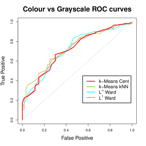
Furthermore, the Bayes factors for colour and grayscale images separate well enough that this model applied to observed sequences of fixations can be used as a weak classifier as to whether or not the subjects are observing an image with colour information. Indeed, over all of the 60 pictures and 3 colour schemes, 14 normals, 13 abnormals, but only 1 grayscale picture scored a Bayes factor $<0.01$. The threshold that most separates this data set is $0.2$, which correctly separates 66% of the normals and 71% of the abnormals from the grayscale images. Thresholding the Bayes factor as a classification criterion for whether or not the observed photograph has colour, normal or abnormal, results in the ROC curves of Figure 4. The ROC curves consider clustering with $k$-means where inclusion is based on either proximity to the cluster centre or $k$-nearest neighbours. Two hierarchical clustering methods are also included, which will be discussed more in Section 2.1. Here, ‘true positive’ refers to the percentage of coloured photos with Bayes factor below the threshold and ‘false positive’ for the percentage of grayscale photos below the threshold.

Ultimately, a sequence of ocular fixations in the grayscale case is better modelled as a collection of independent random draws. In contrast, the coloured cases are better modelled as if jumps between interesting regions of the image occur in a Markovian fashion. This suggests that the absence of colour can make it more difficult for subjects to identify and scan through interesting parts of an image.

Figure 3: Density plots of the distribution of $\log_{2}$ Bayes factors for images of each of the three colour schemes. Blue is for normal, green is for abnormal, and red is for grayscale.

Figure 4: ROC curves for thresholding on the Bayes Factor in order to determine whether the photo being viewed is in colour (true positive) or grayscale (false positive). Four clustering methods are plotted with similar results.

2.1 Clustering methods

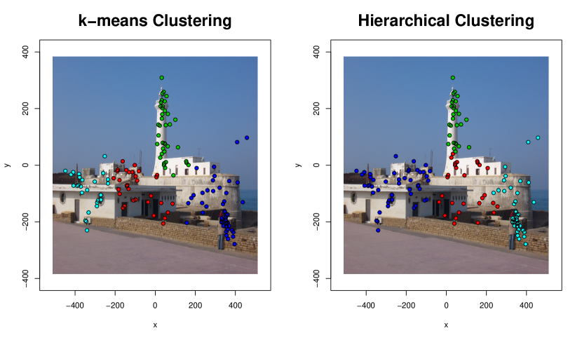
The use of $k$-means clustering with Euclidean distance puts an heavy assumption on our model. Specifically, this approach partitions a photograph into Voronoi cells, which are by design all convex polygons. This approach strives to construct spherical and similarly sized clusters specifically removing the possibility of non-convex or nested clusters. In light of this, a variety of agglomerative hierarchical clustering methods were also tested. For example, Figure 5 depicts $k$-means clustering of the fixations of image 25 using Euclidean distance on the left and complete-linkage hierarchical clustering using the Manhattan or $L^{1}$ distance of those same fixations on the right resulting in different clusters forming.

This “bottom-up” hierarchical clustering begins with each fixation occupying its own cluster. The method iteratively combines clusters based on a combining criterion and an underlying metric. In our analysis, the chosen metrics to test were the Manhattan or $L^{1}$, the Euclidean or $L^{2}$, and the maximum or $L^{\infty}$ distances. The linkage methods chosen were Ward’s minimum variance method, Ward (1963) and Murtagh and Legendre (2014), complete linkage clustering, and unweighted pair group method with arithmetic mean (UPGMA), Sokal and Michener (1958). See Section 14.3 of Hastie et al. (2005) or Section 8.5 of Legendre and Legendre (2012) for an overview of such methods.

Of the various combinations of such metrics and linkage criteria, none performed noticeably better than $k$-Means, and many combinations performed worse. The ROC curves in Figure 4 include two for Ward’s method with $L^{\infty}$ and $L^{1}$ distances. As the clusters formed via hierarchical clustering need not be convex, $k$-nearest neighbours was used to determine to which cluster a given fixation from the testing set belonged with a variety of $k$ tested.

Figure 5: A comparison of $k$-means and hierarchical clustering.

2.2 Analysis of transitions

As a specific example, we will consider image 25 under the normal colour scheme, which is displayed in Figure 2. Running the above analysis yielded a decisively strong Bayes factor of 0.0009 in favour of the $k=4$ model over the $k=1$ model. The states are coloured red, green, cyan, purple moving left to right across the image.

For each of the ten subjects, the maximum likelihood estimate of the initial probabilities and transition matrix from the Dirichlet posteriors were averaged into the following:

$$\pi= \begin{pmatrix}\,\,0.05&0.45&0.13&0.37\,\end{pmatrix},$$

$$p= \begin{pmatrix}0.51&0.29&0.14&0.06\\ 0.30&0.26&0.24&0.20\\ 0.07&0.18&0.58&0.18\\ 0.05&0.11&0.13&0.70\end{pmatrix}.$$

Here, states 1, 3, and 4 fall into the often seen pattern of having probability higher than 50% of remaining in the same state and of having other transition probabilities that roughly decrease as the distance between clusters increases.

2.3 Analysis of saccade length

We now investigate the saccades, which are the distances between successive fixations. We make use of the Euclidean distance of the fixations on a plane for the following analysis. In Ho-Phuoc et al. (2012), saccades are instead measured with an angular metric.

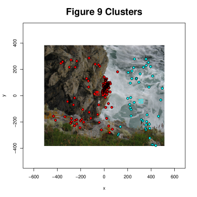
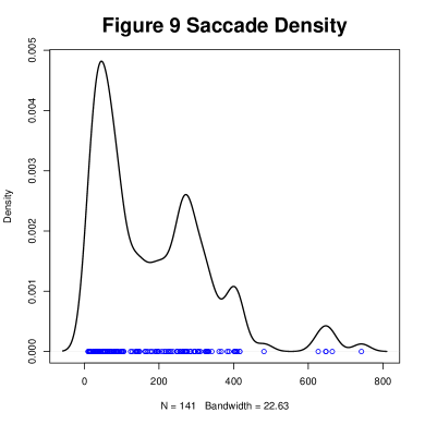
For images that strongly fit the above Markov model, the saccades follow a natural mixture model. For example, if the Markov point process is supported on two states, then the eye can choose to stay in the same state (i.e. a short saccade) or transition to the other state (i.e. a long saccade). This behaviour is readily evident in Figure 6, which displays the two clusters of fixations for image 9 on the left and a kernel density estimate for the distribution of the saccade lengths on the right. The KDE was computed with a Gaussian kernel using the Sheather-Jones method of bandwidth selection, Sheather and Jones (1991).

Figure 6: On the left, two clusters of fixations. On the right, a kernel density plot of the saccade lengths.

The saccades, however, contain further information than just reinforcing the Markovian structure of the data. As reported in Ho-Phuoc et al. (2012), a Kolmogorov-Smirnov (KS) test comparing the empirical distributions of the saccades across all images between the normal and abnormal colour schemes yields a significant p-value. Under our use of Euclidean distance, the following are the three p-values for the three KS tests:

Norm - Abno: $$~{}p=0.0163, ~{}p=0.394, ~{}p=0.116$$ Norm - Gray: Abno - Gray:

Going further, we normalise the saccades of each of the 30 subjects by subtracting the subject’s sample mean and dividing by the sample standard deviation. The goal is to remove inter-subject variability from the data in order to focus only on the between colour scheme variation. The following p-values are from the KS test on the normalised saccades.

Norm - Abno: $$~{}p=0.0264, ~{}p=0.0471, ~{}p=0.788$$ Norm - Gray: Abno - Gray:

The main point of interest is the significant difference between the saccades under the normal and abnormal colour schemes. In the previously detailed Markov model, there is no discernible difference between these two settings. Hence, a further understanding of the differences in the saccades could enhance the Markov model.

2.4 The best and the worst

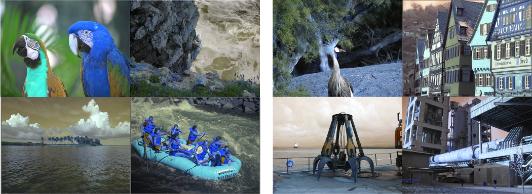
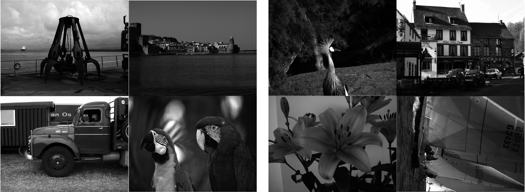
Using the strongest Bayes factor for each photograph, we can rank the photos in order of which best fits the Markov model for $k\geq 2$ clusters. The four best and worst photos for each colour scheme are depicted in Figure 7. The normal coloured images are reasonably partitioned as the worst scoring images contain a singular point of focus whereas the best scorers contain multiple objects on which to fixate such as text and people. The abnormal setting gives similar results barring the photo of eight people in a raft, which scores strongly under normal colours but produced the single worst score under the abnormals. Presumably, the abnormal colour scheme most disorients the brain when it is applied to objects with a narrow range of expected colours such as human faces, which are generally not blue.

Figure 7: The four worst scoring pictures on the left and the four best scoring pictures on the right for the three colour schemes.

3 Extensions

In the following subsections, extensions to the Markov model, which were not fully investigated, are detailed. Each, if incorporated correctly, has the potential to add a great deal of insight into our model.

3.1 Continuous time setting

Perhaps the most blatant omission from the previously described model is the time spent at each fixation. A clever model of the fixation durations would allow for the construction of a continuous time Markov process adding more depth to the model. Evidence suggests that the colour scheme, the fixation location, and the amount of time spent staring at the photograph all contribute to the fixation duration.

First, there are notable differences in the fixation durations under the three colour schemes. In the article of Ho-Phuoc et al. (2012), Kolmogorov-Smirnov tests were run between each pair of empirical distributions for the overall fixations durations. They report no significant difference between the normal and abnormal settings, but report high significance between the grayscale and each of the coloured settings. Furthermore, the distribution of the fixation durations is shown to be non-stationary in time. That is, the distribution of initial durations differs from the distribution of later durations.

From our own investigations, we ask how fixation duration correlates with what is being observed? To answer this, a two dimensional density estimate based on the fixation durations of nine of the ten subjects was used as a data-driven measure of how interesting a region of a given photograph is. Computing the correlation between the density estimate at each fixation point and the duration of tenth subject’s fixation at that point gave the following nontrivial value of 0.1838. The associated 95% confidence interval is $[0.1721,0.1954]$. This demonstrates that the fixation durations of previous subjects can indeed provide useful predictive information about the fixation times for future subjects.

Due to the finite time each picture was displayed, one can also analyse fixation duration by considering its inverse relationship with respect to the total number of fixations per subject per image. The number of fixations per subject per image were tallied and partitioned into three sets for normal, abnormal, and grayscale colour. The box plot in Figure 8 depicts the spread of the three sets of data. It is visibly evident that the normal colour scheme results in a much tighter grouping than the others. Due to the discreteness of the data, the equality of means was tested with the Kruskal-Wallis test, which returned a $p$-value less than $10^{-15}$. Comparing the three pairs via the Mann-Whitney tests resulted in $p$-values:

Norm - Abno: $$~{}p=0.657, ~{}p<10^{-15}, ~{}p=4\times 10^{-11}$$ Norm - Gray: Abno - Gray:

This demonstrates that on average there were fewer fixations made on the grayscale images. In agreement with our results above, this suggests that the lack of colour information resulted in longer fixations and fewer in total as the eye took more time to understand what it was viewing.

Figure 8: Box plots of the total number of fixations partitioned based on subject and condition.

3.2 Image driven analysis

Rather than relying on the data to construct clusters, one could look to the image itself. First and foremost, there has been a considerable amount of research on saliency maps such as Kümmerer et al. (2014) who take inspiration from computer vision and use deep neural networks to determine the eye-catching parts of an image. Beyond computer vision and saliency, there is a vast literature on image segmentation. Ultimately a multifaceted model could be used to partition an image into distinct regions of interest. Such a model may include image gradient information to identify sharp edges and corners that draw the eye as well as specific object recognition to mimic the human eye’s affinity for identifying human faces or written words, which will demand more fixations.

4 Summary and Discussion

Ocular fixation data yields both a challenging and useful analysis. We demonstrated that in the presence of colour information, a sequence of fixations from a human eye can be modeled as a Markov point process. Furthermore, this model breaks down when such colour information is removed from the image. Given that we believe this model, a thorough analysis of the Dirichlet posteriors could yield interesting insight as to how different photographs are treated by the human eye.

This model has the potential to lead to future applications such as a passive diagnostic test for sudden loss of colour vision. That is, even with the 60 miscellaneous photographs of the given data set, it is still possible to roughly classify which observers are looking at colour images and which are not. With a carefully constructed set of colour photographs to elicit Markovian eye movements, one could then use collected data from healthy eyes to train a classifier to determine whether a patient can see colour or not with no other active participation from the patient besides staring at the set of diagnostic photographs.

Ultimately, there is much room for further analysis. The saccade lengths hint at differences between how the eye handles normal versus abnormal colour schemes. Successful integration of the the temporal information will lead to a more comprehensive model. Attempting to construct such a model from image information rather than fixation data could offer insight into saliency maps and lead to more complex and interesting Markov states than the convex polygons from the $k$-means approach.

5 Acknowledgments

The authors would like to acknowledge the Young Statisticians Section and Research Section of the Royal Statistical Society and the contest sponsor, Select Statistics, for constructing a very fun and intellectually exciting Statistical Analytics Challenge.

References

- Baddeley and Tatler (2006) Baddeley, R. J. and Tatler, B. W. (2006) High frequency edges (but not contrast) predict where we fixate: A bayesian system identification analysis. Vision research, 46, 2824–2833.
- Barthelmé et al. (2013) Barthelmé, S., Trukenbrod, H., Engbert, R. and Wichmann, F. (2013) Modeling fixation locations using spatial point processes. Journal of vision, 13, 1.
- Diggle (2003) Diggle, P. J. (2003) Statistical analysis of spatial point patterns. Academic press.
- Frey et al. (2008) Frey, H.-P., Honey, C. and König, P. (2008) What’s color got to do with it? the influence of color on visual attention in different categories. Journal of Vision, 8, 6–6.
- Good (1967) Good, I. J. (1967) A bayesian significance test for multinomial distributions. Journal of the Royal Statistical Society. Series B (Methodological), 399–431.
- Hamel et al. (2014) Hamel, S., Guyader, N., Pellerin, D. and Houzet, D. (2014) Color information in a model of saliency. In Signal Processing Conference (EUSIPCO), 2014 Proceedings of the 22nd European, 226–230. IEEE.
- Hastie et al. (2005) Hastie, T., Tibshirani, R., Friedman, J. and Franklin, J. (2005) The elements of statistical learning: data mining, inference and prediction. The Mathematical Intelligencer, 27, 83–85.
- Ho-Phuoc et al. (2012) Ho-Phuoc, T., Guyader, N., Landragin, F. and Guérin-Dugué, A. (2012) When viewing natural scenes, do abnormal colors impact on spatial or temporal parameters of eye movements? Journal of Vision, 12, 4.
- Illian et al. (2008) Illian, J., Penttinen, A., Stoyan, H. and Stoyan, D. (2008) Statistical analysis and modelling of spatial point patterns, vol. 70. John Wiley & Sons.
- Kass and Raftery (1995) Kass, R. E. and Raftery, A. E. (1995) Bayes factors. Journal of the American Statistical Association, 90, 773–795.
- Kümmerer et al. (2014) Kümmerer, M., Theis, L. and Bethge, M. (2014) Deep gaze i: Boosting saliency prediction with feature maps trained on imagenet. arXiv preprint arXiv:1411.1045.
- Legendre and Legendre (2012) Legendre, P. and Legendre, L. F. (2012) Numerical ecology, vol. 24. Elsevier.
- McLachlan and Peel (2004) McLachlan, G. and Peel, D. (2004) Finite mixture models. John Wiley & Sons.
- Murtagh and Legendre (2014) Murtagh, F. and Legendre, P. (2014) Ward’s hierarchical agglomerative clustering method: which algorithms implement ward’s criterion? Journal of Classification, 31, 274–295.
- Sheather and Jones (1991) Sheather, S. J. and Jones, M. C. (1991) A reliable data-based bandwidth selection method for kernel density estimation. Journal of the Royal Statistical Society, Series B, 53, 683–690.
- Sokal and Michener (1958) Sokal, R. R. and Michener, C. D. (1958) A statistical method for evaluating systematic relationships. University of Kansas Scientific Bulletin, 28, 1409–1438.
- Ward (1963) Ward, J. H. (1963) Hierarchical grouping to optimize an objective function. Journal of the American statistical association, 58, 236–244.