Generation of Electrojets in Weakly Ionized Plasmas through a Collisional Dynamo

Abstract

Intense electric currents called electrojets occur in weakly ionized magnetized plasmas. An example occurs in the Earth’s ionosphere near the magnetic equator where neutral winds drive the plasma across the geomagnetic field. Similar processes take place in the Solar chromosphere and MHD generators. This letter argues that not all convective neutral flows generate electrojets and it introduces the corresponding universal criterion for electrojet formation, $\nabla\times(\mathbf{U}\times\mathbf{B})\neq\partial\mathbf{B}/\partial t$, where $\mathbf{U}$ is the neutral flow velocity, $\mathbf{B}$ is the magnetic field, and $t$ is time. This criterion does not depend on the conductivity tensor, $\hat{\sigma}$. For many systems, the displacement current, $\partial\mathbf{B}/\partial t$, is negligible, making the criterion even simpler. This theory also shows that the neutral-dynamo driver that generates electrojets plays the same role as the DC electric current plays for the generation of the magnetic field in the Biot-Savart law.

A weakly ionized plasma in a strong magnetic field, colliding with a neutral gas, can generate electric currents called electrojets. One such neutral-driven electrojet, named the equatorial electrojet, forms in the Earth’s E-region ionosphere around the magnetic equator Rishbeth (1997); Forbes (1981); Heelis (2004); Kelley (2009). This electrojet results from a large $\mathbf{E}$-field that ultimately derives its energy from neutral winds, abundant in the bottom of the thermosphere (90 - 130 km altitude). The resulting $\mathbf{E}\times\mathbf{B}$ drifting electrons cause the primary electrojet current. Similar electrojets exist along the magnetic equators of other magnetized planets Raghavarao and Dagar (1983). Strong convective neutral flows across $\mathbf{B}$ in the highly collisional solar chromosphere will also generate electrojets Fontenla (2005); Fontenla et al. (2008); Madsen et al. (2014). Under special conditions, similar processes can take place in magnetohydrodynamic (MHD) generators Rosa et al. (1991); Bokil et al. (2015). This paper presents a novel approach in analyzing the strength of electrojets and develops a universal criterion for the existence of these currents. It also shows that the simple 1D model often used by textbooks and papers to illustrate the origin of electrojets will not, in fact, create an electrojet.

Electrojets develop a complex array of behaviors beyond just generating currents strong enough to cause large magnetic field perturbations. These currents also frequently drive various plasma instabilities that result in plasma density irregularities and fluctuating electric fields Farley (2009). These irregularities and fields have been observed for a long time by radars and rockets Kelley (2009); Pfaff (2012). These instabilities can cause intense electron heating and anomalous conductivities Schlegel and St.-Maurice (1981); Foster and Erickson (2000); Dimant and Milikh (2003); Dimant and Oppenheim (2011). Fontenla (2005) has speculated that such instabilities may play an important role in chromospheric heating.

Theoretical studies of the Earth’s equatorial electrojet have a long history Bramley (1967); Krylov et al. (1974); Richmond (1973); Forbes and Lindzen (1976), providing detailed quantitative descriptions of the electrodynamic effects due to different components of the neutral wind. However, they have never addressed the following simple questions: 1) Do the neutral convection flows always drive electrojets? and 2) What component of the winds drive electrojet formation? We answer these fundamental questions in this letter. We provide a simple universal criterion for wind-driven electrojets and identify the driving components of the wind. We demonstrate that this driver plays the same role in electrojet formation as does the DC electric current in the generation of magnetic field via the Biot-Savart law.

Auroral electrojets, found at high latitudes of magnetized planets, result from externally imposed electric fields that propagate along field lines from well outside the electrojet region. The neutral wind has only modest effects on these electrojets and this analysis does not apply.

Electrojets form in plasmas where the neutral density is sufficient to collisionally demagnetize the ions, $\Omega_{i}\ll\nu_{i}$, but not the electrons, $\Omega_{e}\gg\nu_{e}$, where $\Omega_{e,i}$ are the electron/ion gyrofrequencies and $\nu_{e,i}$ are the electron-neutral/ion-neutral collision frequencies. In a spatially inhomogeneous plasma, the convective neutral flow affects each species differently, resulting in a small charge separation. This generates an ambipolar electrostatic field that leads to the formation of electrojets, provided the conditions derived herein are satisfied.

This analysis focuses on large-scale and slow evolution, and so assumes a weakly ionized, inertialess, cold, and quasineutral plasmas. This leads to the following dynamo equations,

$$\nabla\cdot\mathbf{J}=0,\qquad\mathbf{J}=\hat{\sigma}(\mathbf{E}+\mathbf{U}\times\mathbf{B}),$$ (1)

where $\mathbf{J}\equiv\sum_{\alpha}q_{\alpha}n_{\alpha}\mathbf{V}_{\alpha}$ is the total plasma current density, $q_{\alpha}$, $n_{\alpha}$, and $\mathbf{V}_{\alpha}$ are respectively the charge, particle density, and mean fluid velocity of species $\alpha$, which includes including multiple ion species and electrons. In Eq. (1), $\hat{\sigma}$ is the anisotropic conductivity tensor determined in the local frame of reference of the neutral flow, $\mathbf{E}$ and $\mathbf{B}$ are the total DC electric and magnetic fields, and $\mathbf{U}$ is the convective velocity of the neutral gas Kelley (2009).

Now we will obtain a simple criterion for electrojet formation. The $\mathbf{U}\times\mathbf{B}$ term in eq. (1) underlies neutral-dynamo driven electrojets. The neutral flow and magnetic field are usually decoupled, so that $\mathbf{U}\times\mathbf{B}$ can form a general vector field. In the simplest case, one can assume that the magnetic field is stationary, $\partial\mathbf{B}/\partial t=0$, and the dynamo term is irrotational, $\nabla\times(\mathbf{U}\times\mathbf{B})=0$, so that $\mathbf{U}\times\mathbf{B}=-\nabla\Psi$. In this case, Eq. (1) becomes $\mathbf{\nabla}\cdot\hat{\sigma}(\mathbf{\nabla}\Phi+\mathbf{\nabla}\Psi)=0$, where $\Phi$ is the electrostatic potential. One solution exists when $\Phi=-\Psi$. This is a unique stable solution when $\Phi=-\Psi=0$ on the boundaries. A proof of this is beyond the scope and scale of this paper.

This means that, for a plasma embedded in a dense neutral flow with a large collisional momentum exchange, the frictional forces reduce the differences between the convection velocities of the neutral gas and plasma. The resulting $\mathbf{E}$-field creates a quasi-neutral plasma flow that satisfies $\mathbf{E}+\mathbf{U}\times\mathbf{B}=0$. Physically, this means that there is no difference between the mean fluid velocities, $\mathbf{V}_{e}=\mathbf{V}_{i}=\mathbf{U}$, resulting in $\mathbf{J}=0$. This state is achieved for an arbitrary conductivity tensor, $\hat{\sigma}$. For magnetized electrons and unmagnetized ions, such a plasma becomes ‘frozen’ into the neutral flow during a short relaxation time, $\tau_{\mathrm{rel}}\sim\max[\Omega_{e}^{2}/(\nu_{e}\omega_{pe}^{2}),\ \nu_{i}^{-1}]$, where $\omega_{pe}$ is the electron plasma frequency. In this frozen flow, the motion of magnetized electrons is sustained by the $\mathbf{E}\times\mathbf{B}$ drift, while the ion motion is sustained mostly by ion-neutral collisions.

For the case when

$$\nabla\times(\mathbf{U}\times\mathbf{B})\neq 0,$$ (2)

no charge separation can create an electric potential that perfectly matches the neutral drag and, hence, completely cancels the current. Therefore, Eq. (2) represents the criterion for driving an electrojet by a neutral dynamo with stationary $\mathbf{B}$. This criterion is valid for an arbitrary conductivity tensor and has to be fulfilled at least somewhere within the conducting plasma.

The Eq. (2) criterion is easily extended to non-stationary $\mathbf{B}$. Separating the total electric field $\mathbf{E}$ into inductive, $\mathbf{E}_{\mathrm{ind}}$, and electrostatic, $-\nabla\Phi$, parts, and using Faraday’s equation, we obtain the inequality

$$\nabla\times(\mathbf{U}\times\mathbf{B})\neq\frac{\partial\mathbf{B}}{\partial t},$$ (3)

that gives the general condition for a neutral dynamo to drive electrojets.

This general criterion stays the same even after including the plasma pressure and gravity – factors neglected in the standard dynamo described by Eq. (1). A weakly ionized plasma behaves as an isothermal gas, such that the pressure terms in the fluid momentum equations, $-\nabla P_{\alpha}/n_{\alpha}$, can be expressed as $-\nabla\left(T_{\alpha}\ln n_{\alpha}\right)$. Since the gravity force is always the gradient of a gravitational potential, both the pressure terms and gravity can be expressed as gradients of scalar functions which can be combined with $\Phi$ with no consequences for Eq. (3).

In order to better understand the criterion expressed by Eq. (3), we expand its left-hand side in a standard way and apply the continuity equation for the neutral flow, $\partial\rho/\partial t+\nabla\cdot(\rho\mathbf{U})=0$, where $\rho$ is the neutral gas density. Introducing the convective derivative, $D/Dt\equiv\partial/\partial_{t}+\mathbf{U}\cdot\nabla$, Eq. (3) becomes

$$\frac{D}{Dt}\left(\frac{\mathbf{B}}{\rho}\right)\neq\left(\frac{\mathbf{B}}{\rho}\cdot\nabla\right)\mathbf{U}.$$ (4)

This inequality means that the magnetic field is not ‘frozen’ into the neutral flow. Many simple systems will not meet this requirement. For example, an incompressible 2D neutral flow perpendicular to a constant $\mathbf{B}$ cannot generate an electrojet, regardless of the spatial inhomogeneity of the conductivity tensor.

Though Eq. 3 tells us that the curl components of $\mathbf{U}\times\mathbf{B}+\mathbf{E}_{\mathrm{ind}}$ cause electrojets, it does not extract those components. We will now do so. Defining $\mathbf{K}\equiv\mathbf{U}\times\mathbf{B}+\mathbf{E}_{\mathrm{ind}}$, we simplify Eq. (3) to $\nabla\times\mathbf{K}\neq 0$. The Helmholtz decomposition of $\mathbf{K}$, assuming that $\mathbf{K}(\mathbf{r},t)$ vanishes at infinity sufficiently rapidly Arfken and Weber (2005), gives

$$\mathbf{K}(\mathbf{r},t)=-\ \nabla\Psi+\nabla\times\mathbf{A},$$ (5)

where the scalar and vector ‘potentials’ are given by 3D volume integrals

$$\Psi(\mathbf{r},t)=\frac{1}{4\pi}\int\frac{\nabla^{\prime}\cdot\mathbf{K}(\mathbf{r}^{\prime},t)}{|\mathbf{r}-\mathbf{r}^{\prime}|}\ d^{3}r^{\prime},$$ (6a)

$$\mathbf{A}(\mathbf{r},t)=\frac{1}{4\pi}\int\frac{\nabla^{\prime}\times\mathbf{K}(\mathbf{r}^{\prime},t)}{|\mathbf{r}-\mathbf{r}^{\prime}|}\ d^{3}r^{\prime}.$$ (6b)

Here $\nabla^{\prime}$ indicates that the corresponding vector differentiations are with respect to $\mathbf{r}^{\prime}$. In 2D problems, $d^{3}r^{\prime}/|\mathbf{r}-\mathbf{r}^{\prime}|$ should be replaced by $-\ln(|\mathbf{r}-\mathbf{r}^{\prime}|^{2})d^{2}r^{\prime}$. If we consider a finite volume restricted by the boundary surface $S$, then Eq. (5) holds with slightly modified ‘potentials’. The 3D integrations in Eq. (6b) outside the finite volume are replaced by 2D integrals over the boundary surface with $\nabla^{\prime}$ replaced by $-\hat{n}$, where $\hat{n}(\mathbf{r}^{\prime})$ is the local unit normal to the surface $S$, directed outward.

In the expression for the total current density, $\mathbf{J}=\hat{\sigma}(-\nabla\Phi+\mathbf{K})$, the scalar ‘potential’ $\Psi$ can be combined with the actual electrostatic potential, $\Phi$, into one scalar function, $\Upsilon\equiv\Phi+\Psi$, so that the current density becomes

$$\mathbf{J}=\hat{\sigma}\left(-\nabla\Upsilon+\nabla\times\frac{1}{4\pi}\int\frac{\nabla^{\prime}\times\mathbf{K}(\mathbf{r}^{\prime},t)}{|\mathbf{r}-\mathbf{r}^{\prime}|}\ d^{3}r^{\prime}\right),$$ (7)

where

$$\nabla^{\prime}\times\mathbf{K}(\mathbf{r}^{\prime},t) =\nabla^{\prime}\times(\mathbf{U}\times\mathbf{B})-\frac{\partial\mathbf{B}}{\partial t}$$ (8a)

$$=\rho\left[\frac{D^{\prime}}{Dt}\left(\frac{\mathbf{B}}{\rho}\right)-\left(\frac{\mathbf{B}}{\rho}\cdot\nabla^{\prime}\right)\mathbf{U}\right].$$ (8b)

In the general case, $\mathbf{J}$ is not divergence-free, so that the quasi-neutrality equation $\nabla\cdot\mathbf{J}=0$ leads to a second-order partial differential equation for the unknown scalar function $\Upsilon$,

$$\nabla\cdot\left(\hat{\sigma}\nabla\Upsilon\right)=\nabla\cdot[\hat{\sigma}(\nabla\times\mathbf{A})].$$ (9)

Equation (9) is equivalent to Eq. (1), except that it shows explicitly that $\nabla\times\mathbf{K}=\nabla\times(\mathbf{U}\times\mathbf{B})-\partial\mathbf{B}/\partial t$ plays, for electrojet generation, the same role as DC electric currents play in the Biot-Savart law for magnetic field generation. The gradient of the scalar function $\Upsilon$ is the field that forms electrojets.

In the simplest case of spatial uniformity and an isotropic and unmagnetized conductivity tensor of $\sigma_{ij}=\sigma\delta_{ij}$, the current density $\mathbf{J}$ in Eq. (7) becomes divergence-free with $\Upsilon=0$. When $\nabla\times\mathbf{K}\neq 0$ a current develops with $\mathbf{J}=\nabla\times(-\sigma\mathbf{A}\mathcal{)}$, where $-\sigma\mathbf{A}$ is fully equivalent to the volume integral in the Biot-Savart law.

In the general case of an anisotropic and spatially inhomogeneous conductivity tensor $\hat{\sigma}$, the electrojet generation is more complicated than the magnetic field generation described by the Biot-Savart law. The vector field $\nabla\times\mathbf{K}$, with the corresponding integration in $\mathbf{A}$, represents only the primary source, while the entire electrojet formation undergoes an additional step. For the anisotropic and non-uniform $\hat{\sigma}$, we have $\nabla\cdot[\hat{\sigma}(\nabla\times\mathbf{A})]\neq 0$ in almost all locations. In these locations, the unhindered current $\hat{\sigma}(\nabla\times\mathbf{A})$ would accumulate significant volume charges. As soon as this accumulation starts, a non-uniform electrostatic potential $\Phi=\Upsilon-\Psi$ forms, making the entire current, $\mathbf{J}=\hat{\sigma}\nabla(\Upsilon-\nabla\times\mathbf{A})$, divergence-free and, hence, preventing further charge accumulation. Finding the sustained spatial distribution of the quasi-stationary potential $\Phi$, and hence of the total current density $\mathbf{J}$, requires solving Eq. (1).

Unlike Eq. (1), however, Eq. (9) allows us to identify $\nabla\times\mathbf{K}$ as the actual driver of electrojet formation. Equation (9) provides a smooth transition to $\nabla\times\mathbf{K}=0$ when the ‘vector-potential’ $\mathbf{A}$, and hence the right-hand side of Eq. (9), goes away, resulting in $\Upsilon=0$ and no electrojet. Similar to the electric current in the Biot-Savart law, the electrojet driver $\nabla\times\mathbf{K}$ does not have to be non-zero everywhere. For example, imagine a situation where a closed neutral flow, confined within a small volume, generates an electrojet that occupies a much larger space, like a large-scale magnetic field generated by a localized magnetic dipole.

The criterion for electrojet formation should arise directly from explicit analytical solutions of Eq. (1) or (9). To trace this, we consider three simplified models of electrojets that allow such solutions. These models exhibit some key features of the actual electrojets.

The first model is a generalization of the trivial model presented in some textbooks and review papers Kelley (2009); Farley (2009); Pfaff (2012), and shows that this model doesn’t actually yield electrojets. The second is an axially symmetric model with a geometry similar to MHD generators. The third invokes a more complex magnetic field and is a simplified 2-D approximation of the equatorial electrojet and the solar chromosphere.

The first model is the simplest case that produces an electrojet though, as we will see, not directly at the magnetic equator. We assume a horizontally stratified neutral flow, embedded in a uniform magnetic field $\mathbf{B}=B\cos I\,\hat{e}_{x}+B\sin I\,\hat{e}_{z}$ and $\mathbf{U}=U_{x}(z)\hat{e}_{x}+U_{y}(z)\hat{e}_{y}$. The constant magnetic field $\mathbf{B}$ points in an arbitrary direction with respect to the horizontal plane (the inclination, or ‘dip’ angle), $I$. We require $U_{x,y}(z)\rightarrow 0$ as $z\rightarrow 0,\infty$, while $\mathbf{B}$, $\rho(z)$ and $n(z)$ occupy the entire space. As shown below, the plasma will also form a horizontally stratified flow, so that the vertical profiles of the neutral gas and plasma densities, $\rho(z)$ and $n(z)$, are unaffected by the flows and can be independently specified.

The 1D quasi-neutral equation $\partial J_{z}/\partial z=0$ yields a constant $z$-component of the current density, $J_{z}=J_{z0}$. Assuming no imposed external currents, we set $J_{z}=0$. In a 1D system with no potential on the boundaries, the electric field can only have a vertical component, $E_{z}=-\partial\Phi/\partial z$. Using this information, $\mathbf{J}=\hat{\sigma}(\mathbf{E}+\mathbf{U}\times\mathbf{B})$ becomes

$$J_{x}=\frac{\sigma_{\parallel}\left(\sigma_{\mathrm{H}}U_{x}\sin I+\sigma_{\mathrm{P}}U_{y}\right)}{\sigma_{\parallel}\sin^{2}I+\sigma_{\mathrm{P}}\cos^{2}I}\,B_{z},\qquad J_{y}=\frac{\sigma_{\parallel}\left(\sigma_{\mathrm{H}}U_{y}-\sigma_{\mathrm{P}}U_{x}\sin I\right)\sin I-\left(\sigma_{H}^{2}+\sigma_{P}^{2}\right)\!U_{x}\cos^{2}\!I}{\sigma_{\parallel}\sin^{2}I+\sigma_{\mathrm{P}}\cos^{2}I}\,B_{z},$$ (10)

where $\sigma_{\mathrm{P}}$, $\sigma_{\mathrm{H}}$, and $\sigma_{\parallel}$ are the local Pedersen, Hall, and parallel conductivities, respectively Kelley (2009). Equation (10) is applicable to arbitrary $\hat{\sigma}(z)$. For typical electrojet conditions, $\sigma_{\parallel}\gg\sigma_{\mathrm{H}}\gg\sigma_{\mathrm{P}}$, this local solution shows that $|\mathbf{J}|$ increases sharply at $I\sim(\sigma_{\mathrm{P}}/\sigma_{\parallel})^{1/2}$, but in the vicinity of the magnetic equator ($I\rightarrow 0$) this idealized 1D model predicts no electrojet, in contradiction to what exists in nature. Model 3 gives a reasonable approximation of an equatorial electrojet but requires a non-constant $\mathbf{B}$.

We can now check whether Eq. (10) would predict electrojet formation in accord with the above criterion of Eq. (2) or (4). For any arbitrary neutral gas density, Eq. (4) reduces to $B_{z}(d\mathbf{U}/dz)\neq 0$. This requires a finite $B_{z}=B\sin I\neq 0$, along with a vertical velocity shear, $d\mathbf{U}/dz\neq 0$. This appears to create a contradiction because Eq. (10) does not requires a velocity shear. However, an understanding of boundary conditions resolves this problem. A shear must exist to fulfill the original assumption $U_{x,y}(z)\rightarrow 0$ as $z\rightarrow 0,\infty$ but a non-zero $U$ within the system.

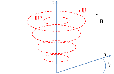
Figure 1: Axially symmetric flow of a neutral gas with possible differential rotation around a vertical uniform magnetic field, $\mathbf{B}$. The dashed red curves schematically show the circular flow lines with some velocities $\mathbf{U}(r,z)$ shown by vectors.

Model 2 is an axially symmetric 2-D system in cylindrical coordinates $r$, $\phi$, $z$ (see Fig. 1) with a uniform vertical magnetic field, $\mathbf{B}$, and a horizontally stratified neutral flow with differential rotation, $U_{\phi}\left(r,z\right)$. For simplicity, we assume that the conductivity is only height-dependent, $\hat{\sigma}=\hat{\sigma}(z)$ ($0<z<\infty$). This problem has relevance to MHD generators Rosa et al. (1991); Bokil et al. (2015).

In the axially symmetric geometry, dynamo Eq. (1) becomes

$$\frac{1}{r}\ \frac{\partial}{\partial r}\left(r[\hat{\sigma}(\mathbf{E}+\mathbf{U}\times\mathbf{B})]_{r}\right)+\frac{\partial J_{z}}{\partial z}=0.$$ (11)

Assuming $\sigma_{\parallel}\gg\sigma_{\mathrm{H},\mathrm{P}}$, we have $J_{z}\approx\sigma_{\parallel}E_{z}$ and $|E_{z}|\ll|E_{r}|$, so that $\Phi(r,z)\approx\Phi_{0}(r)$. Integrating (11) over $z$, under assumption of $\left.J_{z}\right|_{z=0,\infty}=0$, we obtain the dominant radial electric field, $E_{r}(r)=-\left.B\int_{0}^{\infty}\sigma_{\mathrm{P}}U_{\phi}dz\right/\int_{0}^{\infty}\sigma_{\mathrm{P}}dz$, and the corresponding current density,

$$J_{r}(r,z)=\frac{B\sigma_{\mathrm{P}}(z)}{\int_{0}^{\infty}\sigma_{\mathrm{P}}(z^{\prime})dz^{\prime}}\times$$

$$\!\!\!\!\!\!\!\!\!\!\!\!\left(U_{\phi}(r,z)\int_{0}^{\infty}\sigma_{\mathrm{P}}(z^{\prime})dz^{\prime}-\int_{0}^{\infty}\sigma_{\mathrm{P}}(z^{\prime})U_{\phi}(r,z^{\prime})dz^{\prime}\right)\!.$$ (12)

The axial current density is $J_{\phi}=(\sigma_{\mathrm{H}}/\sigma_{\mathrm{P}})J_{r}$. In this approximation, the parallel current, $J_{z}$, is found from the quasi-neutral charge conservation, $\partial J_{r}/\partial r+\partial J_{z}/\partial z=0$, rather than from $J_{z}\approx\sigma_{\parallel}E_{z}$. Simple integration yields:

$$J_{z}=\frac{B}{\int_{0}^{\infty}\sigma_{\mathrm{P}}(z^{\prime})dz^{\prime}}$$ (13)

$$\times \left[\int_{0}^{z}\sigma_{\mathrm{P}}(z^{\prime\prime})dz^{\prime\prime}\int_{0}^{\infty}\sigma_{\mathrm{P}}(z^{\prime})\ \frac{\partial U_{\phi}(r,z^{\prime})}{\partial r}\ dz^{\prime}\right.$$

$$- \left.\ \int_{0}^{\infty}\sigma_{\mathrm{P}}(z^{\prime})dz^{\prime}\int_{0}^{z}\sigma_{\mathrm{P}}(z^{\prime\prime})\ \frac{\partial U_{\phi}(r,z^{\prime\prime})}{\partial r}\ dz^{\prime\prime}\right]\!.$$

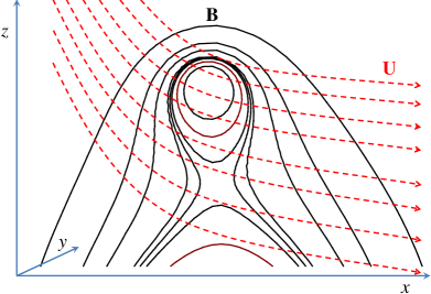
Figure 2: Cartoon of a more general gas flow and magnetic field in the 2D geometry. The solid black curves show the magnetic field lines in the $x,z$-plane, while the dashed red curves show the neutral gas flow lines (the flow velocity $\mathbf{U}$ may have also a $y$-component). The entire structure is invariant along $y$.

The criterion for electrojet formation predicted by Eq. (4) requires just a vertical velocity shear, $\partial U_{\phi}/\partial z\neq 0$. Equations (12) and (13) imply $U_{\phi}=U_{\phi}(r,z)$; otherwise $U_{\phi}(r)$ and $\partial U_{\phi}/\partial r$ could be factored out from all integrals, leading to $\mathbf{J}=0$. This shear does not have to be present in the entire electrojet, only in one or more locations where $\sigma_{\mathrm{P}}$ is not too small.

The last problem is similar to the first except it allows for magnetic field lines arbitrarily distributed in the $x,z$-plane, $\mathbf{B}=\left(B_{x},0,B_{z}\right)$, with $B_{x,z}$ invariant along the $y$-axis (see Fig. 2). In the main region of the weakly ionized plasma, the magnetic field lines can be open or closed (assuming intense localized currents in the $y$ direction). The neutral gas velocity $\mathbf{U}$ may have all three spatial components, invariant along the $y$-axis, $\mathbf{U}=\mathbf{U}(x,z)$. Depending on the specific realization, this model can serve as a reasonable 2D approximation to both the equatorial electrojet and Solar chromosphere.

This geometry suggests introducing curvilinear coordinates, $q_{i}$, where $q_{1}$ specifies a given magnetic field line in the $x,z$-plane, $q_{2}=y$, and $q_{3}$ specifies a location along the given field line. The $q_{2}$ coordinate line is orthogonal to the two others, but the $q_{1}$ and $q_{3}$ coordinate lines are not necessarily orthogonal to each other. We will characterize any vector $\mathbf{S}$ either by its covariant ($S_{i}=\mathbf{S}\cdot\hat{\varepsilon}_{i}$) or contravariant ($S^{i}=\mathbf{S}\cdot\hat{\varepsilon}^{i}$) components, $\mathbf{S}=S_{i}\hat{\varepsilon}^{i}=S^{i}\hat{\varepsilon}_{i}$, repeating subscripts and superscripts implies summation. Here $\hat{\varepsilon}^{i}=\partial q_{i}/\partial\mathbf{r}$ and $\hat{\varepsilon}_{i}=\partial\mathbf{r}/\partial q_{i}$ are the basis vectors related via $\hat{\varepsilon}_{i}=g_{ik}\hat{\varepsilon}^{k}$, where $g_{ik}=\hat{\varepsilon}_{i}\cdot\hat{\varepsilon}_{k}$ is the metric tensor.

In these curvilinear coordinates, Eq. (1) reduces to

$$\frac{\partial}{\partial q_{1}}(\sqrt{g}\,J^{1})+\frac{\partial}{\partial q_{3}}(\sqrt{g}\,J^{3})=0,$$ (14)

where $J^{k}=[\hat{\sigma}(-\nabla\Phi+\mathbf{U}\times\mathbf{B})]^{k}$ and $g\equiv\det\left(g_{ij}\right)=g_{11}g_{33}-g_{13}^{2}$. As in the previous model, using $\sigma_{\parallel}\gg\sigma_{\mathrm{P},\mathrm{H}}$ we obtain $J^{3}\approx\sigma_{\parallel}{(-\nabla\Phi+\mathbf{U}\times\mathbf{B})}_{3}/g_{33}$ and $\Phi(q_{1},q_{3})\approx\Phi_{0}(q_{1})$. To obtain $\Phi_{0}(q_{1})$, we integrate Eq. (14) with respect to $q_{3}$, either over entire closed field lines or over open field lines between sufficiently remote integration limits where $J^{3}\rightarrow 0$. As a result, we obtain

$$\frac{\partial\Phi_{0}}{\partial q_{1}}\approx\frac{\int\left(\sigma_{P}\sqrt{\frac{g_{33}}{g}}\,K_{1}-\sigma_{H}K_{2}\right)dl}{\int\sigma_{P}\sqrt{\frac{g_{33}}{g}}\,dl},$$ (15)

$$J^{1} \approx \frac{\sigma_{P}g_{33}\left(K_{1}\int\sigma_{P}\sqrt{g_{33}/g}\,dl-\int\sigma_{P}K_{1}\sqrt{g_{33}/g}\,dl+\int\sigma_{H}K_{2}dl\right)}{g\int\sigma_{P}\sqrt{g_{33}/g}\,dl}\,-\,\sigma_{H}K_{2}\sqrt{\frac{g_{33}}{g}},$$ (16a)

$$J^{2} \approx \frac{\sigma_{H}\sqrt{g_{33}/g}\left(K_{1}\int\sigma_{P}\sqrt{g_{33}/g}\,dl-\int\sigma_{P}K_{1}\sqrt{g_{33}/g}\,dl+\int\sigma_{H}K_{2}dl\right)}{\int\sigma_{P}\sqrt{g_{33}/g}\,dl}\,+\,\sigma_{P}K_{2},$$ (16b)

where $\mathbf{K}=\mathbf{U}\times\mathbf{B}$ and $dl=\sqrt{g_{33}}\,dq_{3}$ is the length element along $\mathbf{B}$. As in the previous model, $J^{3}$ can be obtained from Eq. (14) by simple integration.

Now we verify that $\nabla\times\mathbf{K}=0$ leads to $\mathbf{J}=0$. Indeed, in this case $\mathbf{K}=\nabla\Psi$, so that $K_{1}=\partial\Psi/\partial q_{1}$ and $K_{2}=0$. This still leaves $J^{1,2}$ with two competing terms $K_{1}\int\sigma_{P}\sqrt{g_{33}/g}\ dl$ and $\int\sigma_{P}K_{1}\sqrt{g_{33}/g}\ dl$, which do not cancel each other if $K_{1}$ depends on $q_{3}$. However, $\mathbf{U}\times\mathbf{B}=\nabla\Psi$ is orthogonal to $\mathbf{B}$, meaning that magnetic field lines are ‘equipotential’ with respect to $\Psi$ (as they are with respect to $\Phi_{0}$). Then $K_{1}=\partial\Psi/\partial q_{1}$ can be factored out from the corresponding integral, resulting in perfect cancellation of the above terms and $J^{1,2}=0$. So, this model also confirms the fact that irrotational $\mathbf{U}\times\mathbf{B}$ cannot form electrojets, whatever the conductivities.

This paper provides a universal criterion for large-scale convective neutral flows to form electrojets in weakly ionized plasmas. This criterion is expressed in two equivalent forms by Eqs. (3) and (4). Although the vector field $\mathbf{U}\times\mathbf{B}$ is the neutral-dynamo term, it is $\nabla\times\mathbf{K}\equiv\nabla\times(\mathbf{U}\times\mathbf{B})-\partial\mathbf{B}/\partial t$ that determines the actual dynamo, as expressed by Eq. (9). This driver plays for generation of the electrojet the same role as the DC electric current plays for generation of the magnetic field (the Biot-Savart law). The above criterion should be taken into account when modeling the neutral dynamo in space or laboratory plasmas.

This work was supported by NSF/DOE Grant PHY-1500439, NASA Grants NNX11A096G and NNX14AI13G, and NSF-AGS Postdoctoral Research Fellowship Award No. 1433536.

References

- Rishbeth (1997) H. Rishbeth, J. Atmos. Solar-Terr. Phys. 59, 1873 (1997).
- Forbes (1981) J. M. Forbes, Reviews of Geophysics and Space Physics 19, 469 (1981).
- Heelis (2004) R. A. Heelis, J. Atmos. Solar-Terr. Phys. 66, 825 (2004).
- Kelley (2009) M. C. Kelley, The Earth’s Ionosphere: Plasma physics and Electrodynamics (Academic Press, Amsterdam, 2009).
- Raghavarao and Dagar (1983) R. Raghavarao and R. Dagar, Planet. Space Sci. 31, 633 (1983).
- Fontenla (2005) J. M. Fontenla, Astronomy and Astrophysics 442, 1099 (2005).
- Fontenla et al. (2008) J. M. Fontenla, W. K. Peterson, and J. Harder, Astronomy and Astrophysics 480, 839 (2008).
- Madsen et al. (2014) C. A. Madsen, Y. S. Dimant, M. M. Oppenheim, and J. M. Fontenla, Astrophys. J. 783, 128 (2014), arXiv:1308.0305 [astro-ph.SR] .
- Rosa et al. (1991) R. J. Rosa, C. H. Krueger, and S. Shioda, IEEE Transactions on Plasma Science 19, 1180 (1991).
- Bokil et al. (2015) V. A. Bokil, N. L. Gibson, D. A. McGregor, and C. R. Woodside, J. of Physics: Conference Series 640, 012032 (2015).
- Farley (2009) D. T. Farley, Ann. Geophys. 27, 1509 (2009).
- Pfaff (2012) R. F. Pfaff, Space Sci. Rev. 168, 23 (2012).
- Schlegel and St.-Maurice (1981) K. Schlegel and J.-P. St.-Maurice, J. Geophys. Res. 86, 1447 (1981).
- Foster and Erickson (2000) J. C. Foster and P. J. Erickson, Geophys. Res. Lett. 27, 3177 (2000).
- Dimant and Milikh (2003) Y. S. Dimant and G. M. Milikh, J. Geophys. Res. 108, 1350 (2003), 10.1029/2002JA009524.
- Dimant and Oppenheim (2011) Y. S. Dimant and M. M. Oppenheim, J. Geophys. Res. (2011).
- Bramley (1967) E. N. Bramley, J. Atmos. Terr. Phys. 29, 1317 (1967).
- Krylov et al. (1974) A. L. Krylov, T. N. Soboleva, D. I. Fishchuk, Y. Y. Tsedilina, and V. P. Shcherbakov, Geomagnetism and Aeronomy 13, 400 (1974).
- Richmond (1973) A. D. Richmond, J. Atmos. Terr. Phys. 35, 1083 (1973).
- Forbes and Lindzen (1976) J. M. Forbes and R. S. Lindzen, J. Atmos. Terr. Phys. 38, 911 (1976).
- Arfken and Weber (2005) J. B. Arfken and H.-J. Weber, Mathematical methods for physicists (Boston: Elsevier, 6th Ed., 2005).