Inference on covariance operators via concentration inequalities: k-sample tests, classification, and clustering via Rademacher complexities

Abstract

We propose a novel approach to the analysis of covariance operators making use of concentration inequalities. First, non-asymptotic confidence sets are constructed for such operators. Then, subsequent applications including a $k$ sample test for equality of covariance, a functional data classifier, and an expectation-maximization style clustering algorithm are derived and tested on both simulated and phoneme data.

1 Introduction

Functional data spans many realms of applications from medical imaging, (Jiang et al., 2014), to speech and linguistics, (Pigoli et al., 2014), to genetics, (Panaretos et al., 2010). General inference techniques for functional data are one area of analysis that has received much attention in recent years from the construction of confidence sets, to other topics such as $k$-sample tests, classification, and clustering of functional data. Most testing methodology treats the data as continuous $L^{2}$ valued functions and subsequently reduces the problem to a finite dimensional one through expansion in some orthogonal basis such as the often utilized Karhunen-Loève expansion (Horváth and Kokoszka, 2012). However, inference in the more general Banach space setting, making use of a variety of norms, has not been addressed adequately. We propose a novel methodology for performing fully functional inference through the application of concentration inequalities; for general concentration of measure results, see Ledoux (2001) and Boucheron et al. (2013). Special emphasis is given to inference on covariance operators, which offers a fruitful way to analyze functional data.

Imagine multiple samples of speech data collected from multiple speakers. Each speaker will have his or her own sample covariance operator taking into account the unique variations of his or her speech and language. An exploratory researcher may want to find natural clusters amidst the speakers perhaps corresponding to gender, language, or regional accent. Meanwhile, a linguist studying the similarities between languages may want to test for the equality of such covariances. A computer scientist may need to implement an algorithm that when given speech data quickly identifies what language is being spoken and furthermore parses the sound clip and identifies each individual phoneme in order to process the speech into text. Our proposed method has the versatility to yield statistical tests that answer these questions as well as others.

Past methods for analyzing covariance operators (Panaretos et al., 2010; Fremdt et al., 2013) rely on the Hilbert-Schmidt setting for their inference. However, the recent work of Pigoli et al. (2014) argues that the use of the Hilbert-Schmidt metric ignores the geometry of the covariance operators and that more statistical power can be gained by using alternative metrics. Hence, we approach such inference for covariance operators in the full generality of Banach spaces, by using a non-asymptotic concentration of measure approach, which has previously been used in nonparametric statistics and machine learning, sometimes under the name of `Rademacher complexities' (Koltchinskii, 2001, 2006; Bartlett et al., 2002; Bartlett and Mendelson, 2003; Giné and Nickl, 2010; Arlot et al., 2010; Lounici and Nickl, 2011; Kerkyacharian et al., 2012; Fan, 2011). These concentration inequalities provide a natural way to construct non-asymptotic confidence regions.

2 Definitions and notation

Generally, we will consider functional data to be in the Hilbert space $L^{2}(I)$ for $I\subset\mathbb{R}$. Our estimated covariance operators of interest are treated as Banach space valued random variables. Let

$$Op(L^{2})=\left\{T:L^{2}(I)\rightarrow L^{2}(I)\,\middle|\,\exists M\geq 0,\left\lVert T\phi\right\rVert_{L^{2}}\leq M\left\lVert\phi\right\rVert_{L^{2}}~{}\forall\phi\in L^{2}(I)\right\}$$

denote the space of all bounded linear operators mapping $L^{2}$ into $L^{2}$. This is where our covariance operators will live.

The metrics that will be investigated are those that correspond to the p-Schatten norms. When $p\neq 2$, these are not Hilbert norms. Hence, we will consider the general Banach space setting.

Definition 2.1 ($p$-Schatten Norm)

Given separable Hilbert spaces $H_{1}$ and $H_{2}$, a bounded linear operator $\Sigma:H_{1}\rightarrow H_{2}$, and $p\in[1,\infty)$, then the $p$-Schatten norm is $\left\lVert\Sigma\right\rVert^{p}_{p}=\mathrm{tr}((\Sigma^{*}\Sigma)^{p/2}).$ For $p=\infty$, the Schatten norm is the operator norm: $\left\lVert\Sigma\right\rVert_{\infty}=\sup_{f\in H_{1}}({\left\lVert\Sigma f\right\rVert_{H_{2}}}/{\left\lVert f\right\rVert_{H_{1}}}).$ In the case that $\Sigma$ is compact, self-adjoint, and trace-class, then given the associated eigenvalues $\{\lambda_{i}\}_{i=1}^{\infty}$, the $p$-Schatten norm coincides with the $\ell^{p}$ norm of the eigenvalues:

$$\left\lVert\Sigma\right\rVert_{p}^{p}=\left\{\begin{array}[]{ll}\left\lVert\lambda\right\rVert_{\ell^{p}}^{p}=\sum_{i=1}^{\infty}\left\lvert\lambda_{i}\right\rvert^{p},&p\in[1,\infty)\\ \max_{i\in\mathbb{N}}\left\lvert\lambda_{i}\right\rvert,&p=\infty\end{array}\right.$$

In order to construct a covariance operator from a sample of functional data, the notion of tensor product is required. Let $f,g\in L^{2}(I)$ and $\phi$ in the dual space $L^{2}(I)^{*}$ with inner product $\left\langle f,\phi\right\rangle=\phi(f)$. The tensor product, $f\otimes g$, is the rank one operator defined by $(f\otimes g)\phi=\left\langle g,\phi\right\rangle f=\phi(g)f$.

Secondly, we will implement a Rademacher symmetrization technique in the concentration inequalities to come. This requires the use of the namesake Rademacher random variables.

Definition 2.2 (Rademacher Distribution)

A random variable $\varepsilon\in\mathbb{R}$ has a Rademacher distribution if $\mathrm{pr}\left(\varepsilon=1\right)=\mathrm{pr}\left(\varepsilon=-1\right)=1/2.$

One particularly fruitful avenue of functional data analysis is the analysis of covariance operators. Such an approach to functional data has been discussed by Panaretos et al. (2010) for DNA microcircles, by Fremdt et al. (2013) for the egg laying practices of fruit flies, and by Pigoli et al. (2014) with application to differentiating spoken languages.

Definition 2.3 (Covariance Operator)

Let $I\subseteq\mathbb{R}$, and let $f$ be a random function (variable) in $L^{2}(I)$ with $\mathrm{E}\left(\left\lVert f\right\rVert_{L^{2}}^{2}\right)<\infty$ and mean zero. The associated covariance operator $\Sigma_{f}\in Op(L^{2})$ is defined as $\Sigma_{f}=\mathrm{E}\left(f^{\otimes 2}\right)=\mathrm{E}\left(\left\langle f,\cdot\right\rangle f\right).$

If $I=\{i_{1},\ldots,i_{m}\}$ has finite cardinality, then $f=(f_{1},\ldots,f_{m})$ is a random vector in $\mathbb{R}^{m}$ and for some fixed vector $v\in\mathbb{R}^{m}$, $\mathrm{E}\left(\left\langle f,v\right\rangle f\right)=\mathrm{E}\left(f{f}^{\mathrm{T}}\right)v$ where $\Sigma_{f}=\mathrm{E}\left(f{f}^{\mathrm{T}}\right)$ is the usual covariance matrix. Covariance operators are integral operators with the kernel function $c_{f}(s,t)=\mathrm{cov}\{{f(s)},{f(t)}\}\in{L^{2}(I\times I)}$. Such operators are characterized by the result that for $f\in L^{2}(I)$, $\Sigma_{f}$ is a covariance operator if and only if it is trace-class, self-adjoint, and compact on $L^{2}(I)$ where the symmetry follows immediately from the definition and the finite trace norm comes from Parseval's equality (Bosq, 2012, Theorem 1.7)(Horváth and Kokoszka, 2012, Section 2.3).

Furthermore, working under the assumption that $\mathrm{E}\left(\left\lVert f\right\rVert_{L^{2}}^{4}\right)<\infty$, we will require tensor powers of covariance operators denoted as $\Sigma^{\otimes 2}:Op(L^{2})\rightarrow Op(L^{2})$. For a basis $\{e_{i}\}_{i=1}^{\infty}\in L^{2}(I)$ with corresponding basis $\{e_{i}\otimes e_{j}\}_{i,j=1}^{\infty}$ for $Op(L^{2}(I))$, the previous definition is extended to $\Sigma^{\otimes 2}=\left\langle\Sigma,\cdot\right\rangle\Sigma$ where for $\Sigma_{1},\Sigma_{2}\in Op(L^{2})$ with $\Sigma_{1}=\sum_{i,j=1}^{\infty}\lambda_{i,j}e_{i,j}$ and $\Sigma_{2}=\sum_{i,j=1}^{\infty}\gamma_{i,j}e_{i,j}$, then $\left\langle\Sigma_{1},\Sigma_{2}\right\rangle=\sum_{i,j}^{\infty}\lambda_{i,j}\gamma_{i,j}$. Specifically for covariance operators, the tensor power takes on a similar integral operator form with kernel $c_{\Sigma}(s,t,u,v)=\mathrm{cov}\left(f(s),f(t)\right)\mathrm{cov}\left(f(u),f(v)\right).$

Given an Hilbert space $H$ with inner product $\left\langle\cdot,\cdot\right\rangle$, the adjoint of a bounded linear operator $\Sigma:H\rightarrow H$, denoted as $\Sigma^{*}$, is the unique operator such that $\left\langle\Sigma f,g\right\rangle=\left\langle f,\Sigma^{*}g\right\rangle$ for $f,g\in H$. The existence of which is given by the Riesz representation theorem (Rudin, 1987, chapter 2). For self-adjoint operators, such as the covariance operators of interest, $\Sigma=\Sigma^{*}$.

We begin with a sample of functional data. Let $f_{1},\ldots,f_{n}\in L^{2}(I)$ be independent and identically distributed observations with mean zero and covariance operator $\Sigma$. Let the sample mean be $\bar{f}={n^{-1}}\sum_{i=1}^{n}f_{i}$ and the empirical estimate of $\Sigma$ be $\hat{\Sigma}=n^{-1}\sum_{i=1}^{n}(f_{i}-\bar{f})\otimes(f_{i}-\bar{f}).$ The initial goal is to construct a confidence set for ${\Sigma}$ with respect to some metric $\mathrm{d}({\cdot},{\cdot})$ of the form $\{{\Sigma}:\mathrm{d}({\hat{\Sigma}},{\Sigma})\leq r(n,\hat{\Sigma},\alpha)\},$ which has coverage $1-\alpha$ for any desired $\alpha\in[0,1]$ and a radius $r$ depending only on the data and $\alpha$. Such a confidence set can be utilized for a wide variety of statistical analyses.

3 Constructing a confidence set

3.1 Confidence sets for the mean in Banach spaces

The goal of this section is to construct a non-asymptotic confidence region in the Banach space setting. These can subsequently be specialized to our case of interest, covariance operators, when the $X_{i}$ below are replaced with $f_{i}^{\otimes 2}$.

The construction of our confidence set is based on Talagrand's concentration inequality (Talagrand, 1996) with explicit constants. This inequality is typically stated for empirical processes (Giné and Nickl, 2016, Theorem 3.3.9 and 3.3.10 ), but applies to random variables with values in a separable Banach space $(B,\left\lVert\cdot\right\rVert_{B})$ as well by simple duality arguments (Giné and Nickl, 2016, Example 2.1.6). Let $X_{1},\ldots,X_{n}\in(B,\left\lVert\cdot\right\rVert_{B})$ be mean zero independent and identically distributed Banach space valued random variables with $\left\lVert X_{i}\right\rVert_{B}\leq U$ for all $i=1,\ldots,n$ where $U$ is some positive constant. Furthermore, let $\left\langle\cdot,\cdot\right\rangle:B\times B^{*}\rightarrow\mathbb{R}$ such that for $X\in B$ and $\phi\in B^{*}$ then $\left\langle X,\phi\right\rangle=\phi(X)$. Define

$$Z =\sup_{\left\lVert\phi\right\rVert_{B^{*}}\leq 1}\sum_{i=1}^{n}\left\langle X_{i},\phi\right\rangle=\left\lVert\sum_{i=1}^{n}X_{i}\right\rVert_{B}, \sigma^{2} =\frac{1}{n}\sum_{i=1}^{n}\sup_{\left\lVert\phi\right\rVert_{B^{*}}\leq 1}\mathrm{E}\left(\left\langle X_{i},\phi\right\rangle^{2}\right),$$

where the supremum is taken over a countably dense subset of the unit ball of $B^{*}$. Furthermore, define $v=2U\mathrm{E}\left(Z\right)+n\sigma^{2}$. Then, $\mathrm{pr}\{{Z}>\mathrm{E}\left(Z\right)+r\}\leq\exp\{{-r^{2}}/({2v+2rU/3})\}.$ Rewriting $Z$ as $n\left\lVert\bar{X}-\mathrm{E}\left(\bar{X}\right)\right\rVert_{B}$ results in

$$\mathrm{pr}\left[\left\lVert\bar{X}-\mathrm{E}\left(\bar{X}\right)\right\rVert_{B}>\mathrm{E}\left\{\left\lVert\bar{X}-\mathrm{E}\left(\bar{X}\right)\right\rVert_{B}\right\}+r\right]<\exp\left(\frac{-n^{2}r^{2}}{2v+2nrU/3}\right)$$

where $\left\lVert X_{i}\right\rVert_{B}<U$ and $v=2nU\mathrm{E}\{\left\lVert\bar{X}-\mathrm{E}\left(\bar{X}\right)\right\rVert_{B}\}+n\sigma^{2}$.

The above tail bound incorporates the unknown $\mathrm{E}(\lVert{\bar{X}-\mathrm{E}\left(\bar{X}\right)}\rVert_{B})$. Consequently, a symmetrization technique is used. This term is replaced by the norm of the Rademacher average $R_{n}={n^{-1}}\sum_{i=1}^{n}\varepsilon_{i}(X_{i}-\bar{X})$ where the $\varepsilon_{i}$ are independent and identically distributed Rademacher random variables also independent of the $X_{i}$. This substitution is justified by invoking the symmetrization inequality (Giné and Nickl, 2016, Theorem 3.1.21),

$$\mathrm{E}\left(Z\right)=\mathrm{E}\left\{\left\lVert\frac{1}{n}\sum_{i=1}^{n}(X_{i}-\mathrm{E}\left(\bar{X}\right))\right\rVert_{B}\right\}\leq 2\mathrm{E}\left\{\left\lVert\frac{1}{n}\sum_{i=1}^{n}\varepsilon_{i}(X_{i}-\bar{X})\right\rVert_{B}\right\}=2\mathrm{E}\left(\left\lVert R_{n}\right\rVert_{B}\right).$$

In practice, the coefficient of $2$ is unnecessary as averaging the data already has a symmetrizing effect, and if starting from symmetric data, then $X-\bar{X}$ and $\varepsilon(X-\bar{X})$ are equal in distribution. This result allows us to replace the original expectation with the expectation of the Rademacher average. Furthermore, Talagrand's inequality also applies to $R_{n}$. Hence, the Rademacher average concentrates strongly about its expectation, which justifies dropping the expectation. In practice, one can use the intermediary $\mathrm{E}_{\varepsilon}\left(\left\lVert R_{n}\right\rVert_{B}\right)$, which can be approximated for reasonable sized data sets via Monte Carlo simulations of the $\varepsilon_{i}$. However, this is not strictly necessary, and for large data sets, a single random draw of $\varepsilon_{i}$ will suffice (Giné and Nickl, 2016, Section 3.4.2).

The resulting $(1-\alpha)$-confidence set is

$$\left\{{X}:\left\lVert{X}-\bar{X}\right\rVert_{B}\leq\left\lVert R_{n}\right\rVert_{B}+\left\{\frac{2}{n}\log(2\alpha)\left(\sigma^{2}+2U\left\lVert R_{n}\right\rVert_{B}\right)\right\}^{1/2}+\frac{U\log(2\alpha)}{3n}\right\}.$$ (3.1)

To make use of these results in practice, both the weak variance $\sigma^{2}$ must be estimated for the data and a reasonable choice of $U$ must be made, and a main contribution of this present paper is to propose some theoretically motivated but practically useful non-asymptotic choices for these constants that work for the functional data applications we are investigating. This will be discussed in the setting of covariance operators in the following subsection.

3.2 Confidence sets for covariance operators

To construct a confidence set for covariance operators, let our functional data $f_{i}\in L^{2}(I)$ and $f_{i}^{\otimes 2}=f_{i}\otimes f_{i}\in Op(L^{2})$, the Hilbert space of bounded linear operators mapping $L^{2}$ to $L^{2}$, such that $(f_{i}\otimes f_{i})\phi=\left\langle f,\phi\right\rangle f$ for some $\phi\in L^{2}$. Hence, for some desired $p$-Schatten norm, $\left\lVert\cdot\right\rVert_{p}$, with $p\in[1,\infty)$ and with conjugate $q=p/(p-1)$, we have

$$Z =\left\lVert\frac{1}{n}\sum_{i=1}^{n}f_{i}\otimes f_{i}-\mathrm{E}\left(f_{i}\otimes f_{i}\right)\right\rVert_{p}=\left\lVert\hat{\Sigma}-\Sigma\right\rVert_{p}, \sigma^{2} =\frac{1}{n}\sum_{i=1}^{n}\sup_{\left\lVert\Pi\right\rVert_{q}\leq 1}\mathrm{E}\left\{\left\langle f_{i}^{\otimes 2}-\mathrm{E}\left(f_{i}^{\otimes 2}\right),\Pi\right\rangle^{2}\right\}$$

for the supremum being taken over a countably dense subset of the unit ball of $\Pi\in Op(L^{2})$. The Rademacher average, $R_{n}={{n^{-1}}\sum_{i=1}^{n}\varepsilon_{i}\{(f_{i}-\bar{f})^{\otimes 2}-\hat{\Sigma}\}},$ is also in $Op(L^{2})$, because for any $\phi\in L^{2}(I)$ and for some $M\in\mathbb{R}$, $\left\lVert R_{n}\phi\right\rVert_{L^{2}}\leq\left\lvert\varepsilon_{i}\right\rvert\lVert{\{(f_{i}-\bar{f})^{\otimes 2}-\hat{\Sigma}\}\phi}\rVert_{L^{2}}\leq M\left\lVert\phi\right\rVert_{L^{2}}$ since $\{(f_{i}-\bar{f})^{\otimes 2}-\hat{\Sigma}\}$ is a bounded operator and $\left\lvert\varepsilon_{i}\right\rvert=1$. Furthermore, in the case that there exists a fixed $c\in\mathbb{R}$ with $\left\lVert f_{i}\right\rVert_{L^{2}}\leq c$ for all $i$ corresponding to a physical bound on the energy of $f_{i}$, $\lVert{f_{i}^{\otimes 2}}\rVert_{p}=\lVert{f_{i}}\rVert_{L^{2}}^{2}\leq c^{2}=U$. It will be determined below that $U\geq\sigma$ in this case. In general, setting $U=\sigma$ gives good experimental results when $f_{i}$ is Gaussian as will be discussed in later sections. This results in $v_{n}\approx\sigma^{2}/n$. For any $p\in[1,\infty)$ and $\alpha\in[0,1/2]$, the proposed $(1-\alpha)$-confidence set inspired by Equation 3.1 for covariance operators is

$$C_{n,1-\alpha}=\left[{\Sigma}:\left\lVert\hat{\Sigma}-{\Sigma}\right\rVert_{p}\leq\left\lVert R_{n}\right\rVert_{p}+\sigma\left\{-\frac{2}{n}\log(2\alpha)\right\}^{1/2}-\frac{\sigma\log(2\alpha)}{3n}\right].$$

where $\sigma$ depends on the distribution on the functional data. As a rule of thumb for the choice of $\sigma^{2}$, as we will now show, is to note that $\sigma^{2}\leq\lVert{\mathrm{E}(f^{\otimes 4})-\Sigma^{\otimes 2}}\rVert_{p}$ and to estimate this bound empirically by $\hat{\sigma}^{2}$. For example, when the $f_{i}$ are from a Gaussian process $\hat{\sigma}\leq{2^{1/2}}\lVert{\Sigma}\rVert_{p}$ as explained in detail in Section 3.4.

To calculate the weak variance $\sigma^{2}$, define $f^{\otimes n}=f\otimes\ldots\otimes f$ to be the n-fold tensor product of $f$ with itself and extend the definition of $\left\langle\cdot,\cdot\right\rangle:(L^{2})^{\otimes 4}\times\{(L^{2})^{\otimes 4}\}^{*}\rightarrow\mathbb{R}$ such that $\left\langle f^{\otimes 4},\phi^{\otimes 4}\right\rangle=\left\langle f^{\otimes 2},\phi^{\otimes 2}\right\rangle^{2}=\left\langle f,\phi\right\rangle^{4}=\phi(f)^{4}.$ For operators $\Pi\in\{(L^{2})^{\otimes 2}\}^{*}$ and $\Xi\in\{(L^{2})^{\otimes 4}\}^{*}$, the weak variance is

$$\sigma^{2} =\frac{1}{n}\sum_{i=1}^{n}\sup_{\left\lVert\Pi\right\rVert_{q}\leq 1}\mathrm{E}\left\{\left\langle f_{i}^{\otimes 2}-\mathrm{E}\left(f_{i}^{\otimes 2}\right),\Pi\right\rangle^{2}\right\}$$

$$\leq\frac{1}{n}\sum_{i=1}^{n}\sup_{\left\lVert\Xi\right\rVert_{q}\leq 1}\left\langle\mathrm{E}\left(f_{i}^{\otimes 4}\right)-\left\{\mathrm{E}\left(f^{\otimes 2}\right)\right\}^{\otimes 2},\Xi\right\rangle\leq\left\lVert\mathrm{E}\left(f^{\otimes 4}\right)-\Sigma^{\otimes 2}\right\rVert_{p}$$

where the inequality stems from the fact that the supremum is being taken over a larger set. However, in the Hilbert space setting, the dual of the tensor product does coincide with the tensor product of the dual space, and thus the above inequality can be replaced with an equality if the Hilbert-Schmidt norm, 2-Schatten norm, is used. Given a bound $\left\lVert f_{i}\right\rVert_{L^{2}}^{2}\leq c^{2}=U$, then $\sigma^{2}\leq\lVert{\mathrm{E}\left(f^{\otimes 4}\right)}\rVert_{p}\leq\mathrm{E}(\lVert{f}\rVert_{L^{2}}^{4})\leq c^{4}=U^{2}.$

3.3 The weak variance for $p=\infty$

Let $E$ be a countable dense subset of the unit ball of $L^{2}(I)$. In the case $p=\infty$, we cannot use duality, but can still write $Z$ and $\sigma^{2}$ as suprema over the countable set and achieve the same results as above.

$$Z =\frac{1}{n}\sup_{e\in E}\sum_{i=1}^{n}\left\langle\left\{f^{\otimes 2}_{i}-\mathrm{E}\left(f^{\otimes 2}_{i}\right)\right\}e,e\right\rangle=\sup_{e\in E}\left\langle(\hat{\Sigma}-\Sigma)e,e\right\rangle=\left\lVert\hat{\Sigma}-\Sigma\right\rVert_{\infty},$$

$$\sigma^{2} =\frac{1}{n}\sum_{i=1}^{n}\sup_{e_{1}\in E}\mathrm{E}\left\{\left\langle(f_{i}^{\otimes 2}-\Sigma)e_{1},e_{1}\right\rangle^{2}\right\}\leq\frac{1}{n}\sum_{i=1}^{n}\sup_{e_{1},e_{2}\in E}\mathrm{E}\left\{\left\langle f_{i}^{\otimes 2}-\Sigma,e_{1}\otimes e_{2}\right\rangle^{2}\right\}$$

$$\leq\frac{1}{n}\sum_{i=1}^{n}\sup_{e_{1},e_{2}\in E}\left\langle\left\{\mathrm{E}\left(f_{i}^{\otimes 4}\right)-\Sigma^{\otimes 2}\right\}(e_{1}\otimes e_{2}),e_{1}\otimes e_{2}\right\rangle=\left\lVert\mathrm{E}\left(f_{i}^{\otimes 4}\right)-\Sigma^{\otimes 2}\right\rVert_{\infty}.$$

As before, if $\left\lVert f_{i}^{\otimes 2}\right\rVert_{\infty}=\left\lVert f_{i}\right\rVert_{L^{2}}^{2}\leq c^{2}=U$, then $\sigma^{2}\leq U^{2}$.

3.4 The weak variance for Gaussian data

Similarly to the bounded case, we estimate $\left\lVert\mathrm{E}\left(f^{\otimes 4}\right)-\Sigma^{\otimes 2}\right\rVert_{p}$ for Gaussian data. Consider $f$ from a Gaussian process with mean zero and covariance $\Sigma$ and define $f_{s}=f(s)$. Strictly speaking these variables are not norm bounded, but similar to concentration results for Gaussian random variables in $\mathbb{R}^{d}$ (Giné and Nickl, 2016, Theorem 3.1.9), we found below that our methods still work well. The integral kernel can be written as (Isserlis, 1918)

$$\mathrm{E}\left(f_{s}f_{t}f_{u}f_{v}\right) =\mathrm{E}\left(f_{s}f_{t}\right)\mathrm{E}\left(f_{u}f_{v}\right)+\mathrm{E}\left(f_{s}f_{u}\right)\mathrm{E}\left(f_{t}f_{v}\right)+\mathrm{E}\left(f_{s}f_{v}\right)\mathrm{E}\left(f_{t}f_{u}\right)$$

$$=c_{f}(s,t)c_{f}(u,v)+c_{f}(s,u)c_{f}(t,v)+c_{f}(s,v)c_{f}(t,u).$$

Hence, we have that $\mathrm{E}\left(f_{s}f_{t}f_{u}f_{v}\right)-\Sigma_{s,t}\Sigma_{u,v}=\Sigma_{s,u}\Sigma_{t,v}+\Sigma_{s,v}\Sigma_{t,u}$ and that the operator $\mathrm{E}\left(f^{\otimes 4}\right)-\Sigma^{\otimes 2}$, which can be thought of as an Hilbert-Schmidt operator on the space $Op(L^{2})$, can be represented by the integral kernel $c_{f}(s,u)c_{f}(t,v)+c_{f}(s,v)c_{f}(t,u)$. These two terms are merely relabeled versions of $\Sigma^{\otimes 2}$. Consequently, using the subadditivity of the norm, $\left\lVert\mathrm{E}\left(f^{\otimes 4}\right)-\Sigma^{\otimes 2}\right\rVert_{p}\leq\left\lVert\Sigma^{\otimes 2}\right\rVert_{p}+\left\lVert\Sigma^{\otimes 2}\right\rVert_{p}=2\left\lVert\Sigma^{\otimes 2}\right\rVert_{p}.$ For example, for the Hilbert-Schmidt norm,

$$\left\lVert\mathrm{E}\left(f^{\otimes 4}\right)-\Sigma^{\otimes 2}\right\rVert^{2}_{HS} =\iiiint\left\{c_{f}(s,u)c_{f}(t,v)+c_{f}(s,v)c_{f}(t,u)\right\}^{2}dsdtdudv$$

$$=2\left\lVert\Sigma\right\rVert^{4}_{HS}+2\iiiint c_{f}(s,u)c_{f}(s,v)c_{f}(t,v)c_{f}(t,u)dsdtdudv\leq 4\left\lVert\Sigma\right\rVert^{4}_{HS}.$$

Lemma 5.1 of Horváth and Kokoszka (2012) gives an explicit form of a covariance operator of $\Sigma$ in terms of the eigenfunctions of $\Sigma$ for Gaussian data in the Hilbert-Schmidt setting.

Given $\lambda_{i}$, the eigenvalues of $\Sigma$, the spectrum of $\Sigma^{\otimes 2}$ is $\{\lambda_{i}\lambda_{j}\}_{i,j=1}^{\infty}$. Hence, for any of the $p$-Schatten norms, $\lVert{\Sigma\otimes\Sigma}\rVert_{p}=\lVert{\Sigma}\rVert_{p}^{2}$. Note that in the above calculations, the weak variance depends on the unknown $\Sigma$. In practice, this can be replaced by the empirical estimate $\hat{\Sigma}$.

4 Applications

4.1 $k$ Sample Comparison

Testing for the equality of means among multiple sets of data is a common task in data analysis. In the functional setting, there has been recent work on performing such a test on covariance operators in order to test whether or not $k$ sets of curves have similar variation. Panaretos et al. (2010) propose such a method for a two sample test on covariance operators given data from Gaussian processes. Similarly, Fremdt et al. (2013) propose a non-parametric two sample test on covariance operators. Both of these approaches make use of the Karhunen-Loève expansion and, hence, the underlying Hilbert space geometry. Pigoli et al. (2014) take a comparative look at a variety of metrics to rank their statistical power when used in a two sample permutation test.

Following from the results of Pigoli et al. (2014), our method uses the $p$-Schatten norms with the concentration inequality based confidence sets of the previous section to compare covariance operators. In the two sample setting, we are able to achieve similar statistical power to that of the permutation test after proper tuning of the coefficients in the inequalities. Furthermore, the analytic nature of the concentration approach leads to a significant reduction in computing time, which offers an even more significant savings for larger values of $k$.

From the confidence set constructed in the previous section, we can devise a test for comparing the empirical covariance operators generated from $k$ samples of functional data. Let the $k$ samples be $f_{1}^{(1)},\ldots,f_{n_{1}}^{(1)},\ldots,f_{1}^{(k)},\ldots,f_{n_{k}}^{(k)}$ where for each sample $i$ and all elements $j=1,\ldots,n_{i}$, $f_{j}^{(i)}$ has covariance $\Sigma^{(i)}$. Our goal is to design a test for the following two hypotheses:

$$\text{H}_{0}: ~{}~{}\Sigma^{(1)}=\ldots=\Sigma^{(k)} \text{H}_{1}: ~{}~{}\exists\,i,j\text{ s.t. }\Sigma^{(i)}\neq\Sigma^{(j)}.$$

To achieve this, a pooled estimate of the weak variance is computed as a weighted average of each sample's individual weak variance in similar style to that of a standard t-test. Let the total data size be $N=n_{1}+\ldots+n_{k}$ and $\sigma_{i}^{2}$ be the weak variance for sample $i$, then the pooled variance is defined as $\sigma_{\text{pool}}^{2}={N^{-1}}\sum_{i=1}^{k}n_{i}\sigma_{i}^{2}.$ Given Gaussian data and the $p$-Schatten norm, for example, this reduces to $\sigma_{\text{pool}}^{2}={2}{N^{-1}}\sum_{i=1}^{k}n_{i}\lVert{\Sigma^{(i)}}\rVert_{p}^{2}$. In practice, $\sigma_{\text{pool}}^{2}$ is estimated from the data for the following confidence regions in order to have those regions only depend on the data.

Taking inspiration from the standard analysis of variance (Casella and Berger, 2002, Chapter 11), let $\hat{\Sigma}^{(i)}$ be the empirical estimate of the covariance operator for the $i$th sample, and let $\hat{\Sigma}$ be the estimate of the covariance operator for the total data set. Making use of the confidence sets for covariance operators from Section 3.2 gives the rejection region

$$\mathcal{C}=\left\{f:\sum_{i=1}^{k}\left\lVert\hat{\Sigma}^{(i)}-\hat{\Sigma}\right\rVert_{p}>\sum_{i=1}^{k}\left\lVert\sum_{j=1}^{n_{i}}\varepsilon_{i,j}\left({f_{j}^{(i)}}^{\otimes 2}-\hat{\Sigma}\right)\right\rVert_{p}+\right.\\ +\left.\left(\sum_{i=1}^{k}\frac{\sigma_{\text{pool}}^{2}}{n_{i}}\right)^{1/2}\left(-2\log 2\alpha\right)^{1/2}+\left(\sum_{i=1}^{k}\frac{\sigma_{\text{pool}}}{n_{i}}\right)\frac{\log 2\alpha}{3}\right\},$$

which under the null hypothesis will have size no greater than the desired $\alpha$.

The size of the test induced by this rejection region is significantly less than the target size $\alpha$ due to the use of multiple concentration inequalities. Hence, tuning the inequalities is required to yield a useful test. Many experiments were run on simulated data sets generated as samples from a Gaussian process with randomly generated covariance operators whose eigenvalues were chosen to decay at a variety of rates. In this setting, the coefficients of $1-k^{-1/2}$ for the Rademacher term and $(k+2)/(k+3)$ for the deviation term were determined experimentally to improve the size of the confidence region:

$$\mathcal{C}=\left[f:\sum_{i=1}^{k}\left\lVert\hat{\Sigma}^{(i)}-\hat{\Sigma}\right\rVert_{p}>\left(1-k^{-1/2}\right)\sum_{i=1}^{k}\left\lVert\sum_{j=1}^{n_{i}}\varepsilon_{i,j}\left({f_{j}^{(i)}}^{\otimes 2}-\hat{\Sigma}\right)\right\rVert_{p}+\right.\\ +\left.\left(\frac{k+2}{k+3}\right)\left\{\left(\sum_{i=1}^{k}\frac{\sigma_{\text{pool}}^{2}}{n_{i}}\right)^{1/2}(-2\log 2\alpha)^{1/2}+\left(\sum_{i=1}^{k}\frac{\sigma_{\text{pool}}}{n_{i}}\right)\frac{\log 2\alpha}{3}\right\}\right].$$ (4.1)

4.2 Classification of Operators

Classification of functional data has been an area of heavy research over the last two decades. James and Hastie (2001) extend linear discriminant analysis to functional data. Hall et al. (2001) and Glendinning and Herbert (2003) classify with principle components. Ferraty and Vieu (2003) implement kernel estimators. General linear models for functional data are discussed by Müller and Stadtmüller (2005). Delaigle and Hall (2012) analyze the asymptotic properties of the centroid based classifier. Wavelet based classification is detailed by Berlinet et al. (2008) and Chang et al. (2014).

One application of our method beyond classification of functional data is the classification of covariance operators. In the setting of speech analysis, consider multiple speakers and multiple samples of speech from each speaker. The speech samples can be combined into a single sample covariance operator for each speaker. Then, our method can be employed, for example, to classify the covariance operators by speaker gender or speaker language. Evidence that this is a fruitful approach can be found in the analysis of Pigoli et al. (2014) and Pigoli et al. (2015) where a variety of metrics are compared for their efficacy when performing inference on covariance operators. These articles detail the discrepancy between sample covariance operators produced by speakers of different romance languages.

Given $k$ possible labels and $n$ samples of labeled data $(Y_{i},f_{i})$ with label $Y_{i}\in\{1,\ldots,k\}$ and observation $f_{i}\in L^{2}(I)$, our goal is to determine the probability that a newly observed $g\in L^{2}(I)$ belongs to label $Y=j$. Given such a $g$, the Bayes classifier chooses the label $y=\arg\max_{j}\mathrm{pr}(Y=j\mid g)$ where $\mathrm{pr}(Y=j\mid g)={\mathrm{pr}(g\mid Y=j)\mathrm{pr}\left(Y=j\right)}/{\mathrm{pr}\left(g\right)}$.

Beginning with a training set of $n$ samples with $n_{j}$ samples of label $j$, the sample mean of each category is computed: $\bar{f}_{j}={n_{j}^{-1}}\sum_{i:Y_{i}=j}f_{i}$. The probability $\mathrm{pr}(g\mid Y=j)$ above is replaced with $\mathrm{pr}[\left\lVert\bar{f}_{j}-g\right\rVert_{L^{2}}>\mathrm{E}\{\left\lVert\bar{f}_{j}-\mathrm{E}\left(\bar{f}_{j}\right)\right\rVert_{L^{2}}\}+r]$ with the goal of making a decision based on how much more $\bar{f}_{j}$ differs from $g$ than $\bar{f}_{j}$ differs from its expectation $\mathrm{E}\left(\bar{f}_{j}\right)$. Similar techniques to those is Section 3 as used. Define the Rademacher sum, $R_{j}$, and the empirical weak variance, $\hat{\sigma}_{j}^{2}$, for label $j$ to be, respectively,

$$R_{j} =\frac{1}{n_{j}}\sum_{i:Y_{i}=j}\varepsilon_{i}(f_{i}-\bar{f}_{j}), \hat{\sigma}_{j}^{2} =\left\lVert\frac{1}{n_{j}}\sum_{i:Y_{i}=j}f_{i}^{\otimes 2}-\bar{f}_{j}^{\otimes 2}\right\rVert_{p}$$

where $\varepsilon_{i}$ are independent and identically distributed Rademacher random variables. The tail bound for the above probability is then

$$\mathrm{pr}\left(\left\lVert\bar{f}_{j}-g\right\rVert_{L^{2}}-\left\lVert R_{j}\right\rVert_{L^{2}}>r\right)<\exp\left(\frac{-n_{j}r^{2}}{4\left\lVert R_{j}\right\rVert_{L^{2}}U+2\hat{\sigma}_{j}^{2}+2rU/3}\right),$$ (4.2)

where $U$ is an upper bound on $\left\lVert f_{i}\right\rVert_{L^{2}}$. However, this can be approximated by the Gaussian tail $\exp\left(-n_{j}r^{2}/2\sigma^{2}_{j}\right).$ In the simulations of Section 5.3, this approximation actually achieves a better correct classification rate on both Gaussian and t-distributed data. This specifically works on t-distributed data as the estimate in Equation 4.3 below is merely concerned with comparing the tail bounds rather than their specific values. Consequently, the tail for every category is underestimated in the t case, but the ratio remains valid for comparison purposes.

Assuming uniform priors on the labels, the estimate for the probability expression in the Bayes classifier is

$$\mathrm{pr}(Y=j\mid g) \approx\frac{\phi_{j}({g})}{\sum_{l=1}^{k}\phi_{l}({g})}, \phi_{j}(g) =\exp\left\{-\frac{n_{j}}{2}\left(\frac{\left\lVert\bar{f}_{j}-g\right\rVert_{L^{2}}-\left\lVert R_{j}\right\rVert_{L^{2}}}{\hat{\sigma}_{j}}\right)^{2}\right\}.$$ (4.3)

This can be extended to the case where an unlabeled observation is a collection of curves $g_{1},\ldots,g_{m}$ by replacing $\lVert{\bar{f}_{j}-g}\rVert_{L^{2}}$ in the above expression with $\lVert{\bar{\Sigma}_{j}-\hat{\Sigma}_{g}}\rVert_{p}$ where $\bar{\Sigma}_{j}$ is the sample covariance of the $f_{i}$ with label $j$ and $\hat{\Sigma}_{g}$ is the sample covariance of the $g_{i}$. The Rademacher and weak variance terms would also be updated accordingly.

4.3 Clustering of Operator Mixtures

Closely related to the problem of classification is the problem of clustering. Given a sample of functional data, we want to assign one of a finite collection of labels to each curve. For example, in speech processing, one may want to cluster sound clips based the language of the speaker, or, to be discussed in Section 5.4, one may want to separate unlabeled phoneme curves into clusters.

There have been many recently proposed methods for clustering functional data. Many approaches begin by constructing a low dimensional representation of the data in some basis such as modelling the data with a B-spline basis followed by clustering the spline representations with k-means (Abraham et al., 2003). A similar approach makes use of the eigenfunctions of the covariance operator instead of B-splines (Peng and Müller, 2008). In contrast, we will attempt to cluster functions or operators directly via a concentration of measure approach similar to the previously described classification procedure.

Consider the same setting to the previous section of multiple observations from multiple categories. However, now the category labels are missing. This is a functional mixture model where each observed functional datum is a stochastic process with one of $k$ possible covariance operators. In the below experiments, the data will be simulated from a Gaussian process. The goal is to correctly separate the data into $k$ sets. To achieve this, an expectation-maximization style algorithm is implemented.

Let the observed operator data be $S_{1},\ldots,S_{n}\in Op(L^{2})$ where each $S_{i}=\text{cov}(f_{1}^{(i)},\ldots,f_{m_{i}}^{(i)})$ is a rank $m_{i}$ operator produced from $m_{i}$ functional observations. Let the latent label variables be $Y_{1},\ldots,Y_{n}\in\{1,\ldots,k\}$. Assuming no prior knowledge on the proportions of data in each category, the algorithm is initialized with the Jeffreys prior for the Dirichlet distribution by randomly generating $\rho_{i,\cdot}^{(0)}\sim\text{Dirichlet}\left(1/2,\ldots,1/2\right),$ the initial probability vector that $\mathrm{pr}(Y_{i}=*\mid f_{i})$.

Assuming $t$ iterations of the algorithm have completed, we have a label probability vector $\rho_{i,\cdot}^{(t)}$ for each of the $n$ observations. Given this collection of vectors, the expected proportions of each category can be estimated as $\tau_{j}^{(t+1)}={n^{-1}}\sum_{i=1}^{n}\mathrm{E}\left(\boldsymbol{1}_{Y_{i}=j}\right)={n^{-1}}\sum_{i=1}^{n}\rho_{i,j}^{(t)}.$ Similarly, a weighted sum of the data, $\hat{\Sigma}_{j}^{(t+1)}$, and a weighted Rademacher sum, $R_{j}^{(t+1)}$, can be used to update the estimated covariance operators for each label $j$:

$$\hat{\Sigma}_{j}^{(t+1)} =\frac{\sum_{i=1}^{n}\rho_{i,j}^{(t)}{S_{i}}}{\sum_{i=1}^{n}\rho_{i,j}^{(t)}}, R_{j}^{(t+1)} =\frac{\sum_{i=1}^{n}\rho_{i,j}^{(t)}\varepsilon_{i}\left({S_{i}}-\hat{\Sigma}_{j}^{(t+1)}\right)}{\sum_{i=1}^{n}\rho_{i,j}^{(t)}}.$$

Lastly, a pooled weak variance is required, which is used in place of each individual category weak variance. Otherwise, in practice, one single category captures all of the data points. By defining the pooled covariance operator as $\hat{\Sigma}_{\text{pool}}^{(t+1)}=\sum_{j=1}^{k}\tau_{j}^{(t+1)}\hat{\Sigma}_{j}^{(t+1)},$ then the pooled weak variance in the Gaussian case, for example, is estimated by $2\lVert{\hat{\Sigma}_{\text{pool}}^{(t+1)}}\rVert_{p}$.

As a result, the label probability vectors $\rho_{i,\cdot}^{(t)}$ can be updated given the $t+1$st collection of estimated covariance operators, Rademacher sums, and the pooled covariance operator. From the previous section, Equation 4.3 can be used to determine $\rho_{i,j}^{(t+1)}=\mathrm{pr}(Y_{i}=j\mid S_{i},\hat{\Sigma}_{1}^{(t+1)},\ldots,\hat{\Sigma}_{k}^{(t+1)}),$ the probability that observation $i$ belongs to the $j$th category. This process can be iterated until a local optimum is reached.

5 Numerical Experiments

5.1 Simulated and phoneme data

To test each of the above three applications, experiments were first run on simulated data. These data sets were generated as observations from Gaussian or t-distributed processes. The covaraiance operators were randomly chosen given a specific decay rate for the eigenvalues.

Secondly, the phoneme data to be tested (Ferraty and Vieu, 2003; Hastie et al., 1995) is a collection of 400 log-periodograms for each of five different phonemes: /A/ as in the vowel of ``dark''; /O/ as in the first vowel of ``water''; /d/ as in the plosive of ``dark''; /i/ as in the vowel of ``she''; /S/ as in the fricative of ``she''. Each curve contains the first 150 frequencies from a 32 ms sound clip sampled at a rate of 16-kHz.

5.2 k Sample Comparison

The above confidence set in Equation 4.1 comparing $k$ samples can be used to refute the null hypothesis that all covariance operators are equal. A two sample permutation test was performed in Pigoli et al. (2014). Given two samples of functional data, $f_{1}^{(1)},\ldots,f_{n}^{(1)}$ and $f_{1}^{(2)},\ldots,f_{m}^{(2)}$ with associated covariance operators $\Sigma^{(1)}$ and $\Sigma^{(2)}$, respectively, the desired hypotheses to test are

$$\text{H}_{0}: ~{}~{}\Sigma^{(1)}=\Sigma^{(2)} \text{H}_{1}: ~{}~{}\Sigma^{(1)}\neq\Sigma^{(2)}.$$

When using a permutation test, the labels are randomly reassigned $M$ times, and each time, the distance between the two new covariance operators is computed. For sufficiently large $M$, this procedure will return the exact significance level of the observations with respect to the data set.

A power analysis was performed between the permutation method and our proposed concentration approach using Equation 4.1. Given two different operators $\Sigma^{(1)}$ and $\Sigma^{(2)}$ and $\gamma\geq 0$, an interpolation between the two operators is constructed as $\Sigma^{(\gamma)}=[(\Sigma^{(1)})^{1/2}+\gamma\{S(\Sigma^{(2)})^{1/2}-(\Sigma^{(1)})^{1/2}\}][(\Sigma^{(1)})^{1/2}+\gamma\{S(\Sigma^{(2)})^{1/2}-(\Sigma^{(1)})^{1/2}\}]^{*},$ where $S$ is an operator minimizing the Procrustes distance, between $\Sigma^{(1)}$ and $\Sigma^{(2)}$, which is $d_{\text{Proc}}(\Sigma^{(1)},\Sigma^{(2)})^{2}=\inf_{S\in U\{L^{2}(I)\}}\lVert{R^{(1)}-R^{(2)}S}\rVert_{2}^{2}$ where $\Sigma^{(i)}=(R^{(i)})(R^{(i)})^{*}$ and $U\left\{L^{2}(I)\right\}$ is the space of unitary operators on $L^{2}(I)$ (Pigoli et al., 2014).

Monte Carlo simulations were run in order to estimate the power of each test. Two operators $\Sigma^{(1)}$ and $\Sigma^{(2)}$ with similar eigenvalue decay were compared. For sample size $n=50$, $\gamma\in\{0,.1,.2,.3,.4,.5\}$, and for sample size $n=500$, $\gamma\in\{0,.05,.1,.15,.2,.25\}$. For each $\gamma$, 5000 samples of size $n$ were generated for $\Sigma^{(1)}$ and $\Sigma^{(\gamma)}$. Equation 4.1 and the permutation method (Pigoli et al., 2014) were both implemented to estimate the empirical power.

Figures 1 and 2 display the results for operators whose eigenvalues decay at a quartic and quadratic rate, respectively. The solid lines indicate the power of the permutation test, and the circle lines indicate the power of our concentration approach. The colors red, green, and blue correspond to the three norms trace, Hilbert-Schmidt, and operator, respectively.

In most cases, the concentration approach is able to achieve the same power to reject the null as does the permutation test. The notable exception is for the trace norm when the eigenvalues decay slowly. The added benefit to the concentration approach is the speed with which it executes. Across all of the Monte Carlo simulations, our concentration approach ran on average 28.14 times faster than the permutation method. This was computed by tracking the amount of computation time each method spent while producing the plots in Figures 1 and 2, which corresponds to $5$ values of $\gamma$, $2$ values of $\alpha$, $3$ different norms, $2$ sample sizes, and $5000$ replications each resulting in 300,000 function calls for both the permutation and concentration methods. Unlike the other norms, the Hilbert-Schmidt norm can be calculated without explicit computation of the eigenvalues. For each evaluation of the permutation test, 100 permutations of the data were generated, which corresponds to 100 random draws and 100 eigenvalue computations. More accuracy would require even more permutations. In comparison, our concentration approach requires only $3k$ eigenvalue computations and no random draws and hence is only dependent on the number of samples regardless of data size or $\alpha$.

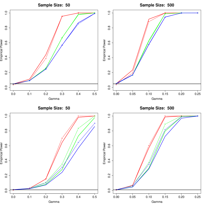
Figure 1: A power analysis for testing whether or not operator $\Sigma^{(1)}=\Sigma^{(\gamma)}$ comparing the permutation method (solid lines) with the concentration approach (circle lines). The size $\alpha=0.05$ in the top row, and $\alpha=0.01$ in the bottom. The eigenvalues of the operators decay at a rate $O(k^{-4})$. The red, green, and blue lines respectively correspond to the trace class, Hilbert-Schmidt, and operator norms.

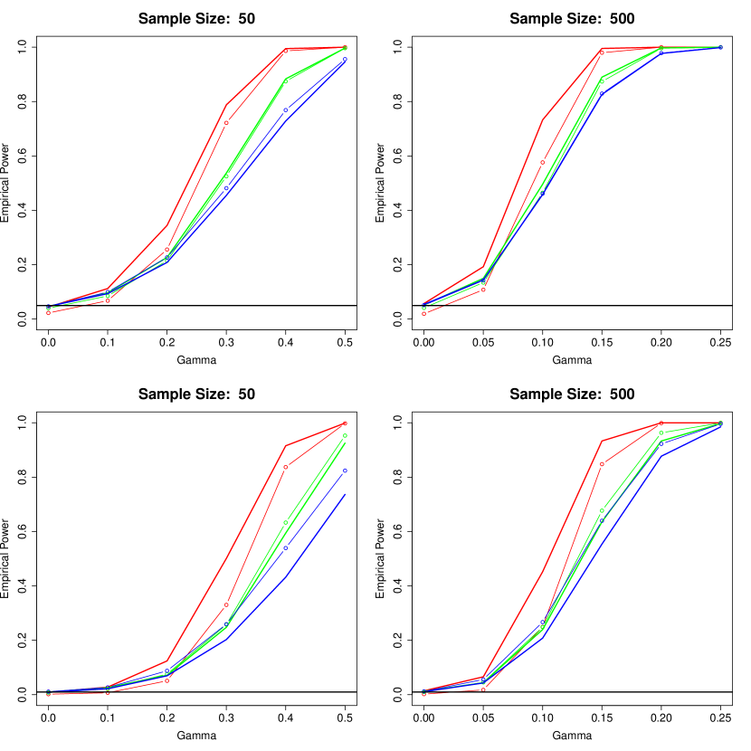
Figure 2: A power analysis for testing whether or not operator $\Sigma^{(1)}=\Sigma^{(\gamma)}$ comparing the permutation method (solid lines) with the concentration approach (circle lines). The size $\alpha=0.05$ in the top row, and $\alpha=0.01$ in the bottom. The eigenvalues of the operators decay at a rate $O(k^{-2})$. The red, green, and blue lines respectively correspond to the trace class, Hilbert-Schmidt, and operator norms.

The proposed $k$-sample test was also used to compare samples of log-periodogram curves from the spoken phonemes /A/ and /O/ . As one can imagine, these vowels can be hard to distinguish; see Section 5.4 for further evidence of this. For $k\in\{2,3,4,5,6\}$, $k-1$ disjoint sets of 40 /A/ curves and one set of 40 /O/ curves were randomly sampled from the data set. This was replicated 500 times, and each time Equation 4.1 was used to decide whether or not the $k$ covariance operators were equivalent at the $\alpha=0.05$ level. The resulting estimated statistical power for each $k$ is

$k$	2	3	4	5	6
Power	0.00	0.018	0.228	0.656	0.936

In the null setting, the above experiement was rerun except that every disjoint set of curves came from the /A/ set. The resulting experimentally computed test sizes are

$k$	2	3	4	5	6
Size	0.00	0.00	0.00	0.004	0.072

5.3 Binary and trinary classification

Our concentration of measure (CoM) method is implemented on covariance operators making use of the trace norm $\left\lVert\cdot\right\rVert_{\text{tr}}$ where for a covariance operator $\Sigma$ with eigenvalues $\{\lambda_{i}\}_{i=1}^{\infty}$, $\left\lVert\Sigma\right\rVert_{\text{tr}}=\sum_{i=1}^{n}\left\lvert\lambda_{i}\right\rvert$. The trace norm was chosen based on the analysis of the preceding section as well as that of Pigoli et al. (2014) where it achieved the best performance when compared with the other p-Schatten norms. The CoM approach to classification of operators is tested in a variety of simulations against other standard approaches to functional classification. The methods used for comparison are $k$-nearest neighbours (Ferraty and Vieu, 2006), classification using kernel estimators (Ferraty and Vieu, 2003), general linear model (Müller and Stadtmüller, 2005), and regression trees.

The first simulation asks each method to classify observed mean zero Gaussian process data or mean zero t-process data with 4 degrees of freedom. The two covariance operators in question, $\Sigma_{1}$ and $\Sigma_{2}$, are the sample covariances of the male and of the females of the Berkeley growth curve data (Ramsay and Silverman, 2005). In particular, $n$ collections of $k$ curves were generated from each of $\Sigma_{1}$ and $\Sigma_{2}$ as a training set, and $m$ collections of $k$ curves were generated as a test set. The CoM method was trained on the set of $n$ sample covariances and used to classify each of the $m$ test covariances. The remaining classification methods were trained and tested in two separate ways: By treating each sample covariance as a function and classifying as usual, and by training on all $n\times k$ observations and testing each of the $m$ collections by classifying each constituent curve individually and taking a majority vote with ties settled by a uniform random draw.

For group sizes $k=1,2,4,8,16$, 100 simulations were run with $n=100$ sets of $k$ training curves. To compare the accuracy of each approach $m=100$ sets of $k$ testing curves were generated for each operator. The accuracy of each method is tabulated in Table 1.

The concentration method performed well against the alternatives. Its performance was on par with the kernel method applied to each covariance operator as a function. Our method was only consistently outperformed by the kernel method implementing the majority vote approach. However, the two operators in question have very similar weak variances. The next simulation demonstrates how the concentration method adapts naturally when the variances of each label significantly differ.

Table 1: A comparison of the performances of five classification methods. The first entry for each method corresponds to classifying the covariance operators as functions. The prime entry corresponds to classifying curves with a majority vote. The estimated percent of correct classification is listed in the table with the sample standard deviation in brackets. The top block comes from Gaussian process data, and the bottom comes from t-process data with 4 degrees of freedom. The highest percentage of each column is marked in bold.

$k$	1	2	4	8	16
CoM	0.62 (0.05)	0.62 (0.05)	0.76 (0.08)	0.87 (0.06)	0.96 (0.03)
KNN	0.52 (0.04)	0.44 (0.04)	0.57 (0.04)	0.76 (0.04)	0.91 (0.02)
KNN′	$\cdot$	0.47 (0.03)	0.59 (0.04)	0.74 (0.03)	0.89 (0.02)
Kernel	0.65 (0.04)	0.64 (0.05)	0.75 (0.03)	0.87 (0.03)	0.96 (0.02)
Kernel′	$\cdot$	0.70 (0.04)	0.82 (0.02)	0.92 (0.02)	0.99 (0.01)
GLM	0.51 (0.04)	0.62 (0.04)	0.74 (0.04)	0.86 (0.02)	0.94 (0.02)
GLM′	$\cdot$	0.50 (0.04)	0.50 (0.03)	0.50 (0.04)	0.50 (0.04)
Tree	0.57 (0.04)	0.54 (0.04)	0.59 (0.03)	0.66 (0.04)	0.75 (0.03)
Tree′	$\cdot$	0.55 (0.04)	0.59 (0.04)	0.60 (0.05)	0.60 (0.09)
CoM	0.59 (0.05)	0.62 (0.05)	0.75 (0.07)	0.86 (0.06)	0.95 (0.04)
KNN	0.42 (0.04)	0.45 (0.04)	0.58 (0.04)	0.76 (0.03)	0.92 (0.02)
KNN′	$\cdot$	0.45 (0.04)	0.58 (0.04)	0.72 (0.03)	0.89 (0.03)
Kernel	0.65 (0.04)	0.64 (0.05)	0.75 (0.04)	0.87 (0.02)	0.96 (0.02)
Kernel′	$\cdot$	0.68 (0.04)	0.80 (0.03)	0.92 (0.02)	0.99 (0.01)
GLM	0.50 (0.03)	0.62 (0.03)	0.74 (0.04)	0.86 (0.03)	0.94 (0.02)
GLM′	$\cdot$	0.50 (0.03)	0.50 (0.03)	0.51 (0.04)	0.50 (0.03)
Tree	0.54 (0.04)	0.54 (0.04)	0.59 (0.03)	0.67 (0.03)	0.75 (0.03)
Tree′	$\cdot$	0.54 (0.04)	0.57 (0.04)	0.59 (0.05)	0.57 (0.06)

CoM, concentration of measure; KNN, k-nearest-neighbours; GLM, generalized linear model; Tree, regression tree.

Continuing from the previous simulation, a third operator is constructed from $\Sigma_{1}$ and $\Sigma_{2}$ by averaging these two and then scaling up the non-principle eigenvalues by a factor of 5. This, in some sense, creates a third operator between the first two, but with higher variance. The simulation is carried out precisely as before, but incorporating all three operators. In this setting, our concentration approach demonstrates the best performance. The results are listed in Table 2.

Table 2: A comparison of the performances of five classification methods as in Table 1, but with three potential classes from which to choose. The estimated percent of correct classification is listed in the table with the sample standard deviation in brackets. The top block comes from Gaussian process data, and the bottom comes from t-process data with 4 degrees of freedom. The highest percentage of each column is marked in bold.

$k$	1	2	4	8	16
CoM	0.51 (0.04)	0.55 (0.04)	0.75 (0.05)	0.89 (0.05)	0.97 (0.03)
KNN	0.50 (0.03)	0.52 (0.03)	0.61 (0.03)	0.75 (0.03)	0.90 (0.02)
KNN′	$\cdot$	0.55 (0.03)	0.68 (0.03)	0.80 (0.02)	0.90 (0.02)
Kernel	0.54 (0.03)	0.52 (0.03)	0.64 (0.03)	0.77 (0.03)	0.92 (0.02)
Kernel′	$\cdot$	0.58 (0.03)	0.69 (0.02)	0.81 (0.03)	0.92 (0.02)
GLM	0.36 (0.04)	0.41 (0.04)	0.49 (0.04)	0.57 (0.03)	0.65 (0.03)
GLM′	$\cdot$	0.35 (0.04)	0.36 (0.04)	0.36 (0.05)	0.35 (0.05)
Tree	0.44 (0.03)	0.44 (0.03)	0.45 (0.03)	0.50 (0.03)	0.55 (0.03)
Tree′	$\cdot$	0.46 (0.03)	0.51 (0.04)	0.51 (0.07)	0.47 (0.07)
CoM	0.46 (0.05)	0.50 (0.06)	0.63 (0.05)	0.75 (0.08)	0.85 (0.07)
KNN	0.46 (0.03)	0.49 (0.03)	0.57 (0.03)	0.67 (0.03)	0.78 (0.02)
KNN′	$\cdot$	0.50 (0.03)	0.64 (0.03)	0.77 (0.02)	0.87 (0.02)
Kernel	0.50 (0.03)	0.48 (0.03)	0.57 (0.03)	0.68 (0.03)	0.80 (0.02)
Kernel′	$\cdot$	0.53 (0.03)	0.66 (0.03)	0.77 (0.02)	0.85 (0.02)
GLM	0.35 (0.03)	0.41 (0.04)	0.46 (0.04)	0.53 (0.03)	0.58 (0.04)
GLM′	$\cdot$	0.35 (0.03)	0.36 (0.04)	0.36 (0.04)	0.36 (0.06)
Tree	0.42 (0.03)	0.44 (0.03)	0.45 (0.03)	0.46 (0.03)	0.49 (0.03)
Tree′	$\cdot$	0.43 (0.03)	0.47 (0.04)	0.48 (0.06)	0.46 (0.08)

CoM, concentration of measure; KNN, k-nearest-neighbours; GLM, generalized linear model; Tree, regression tree.

These five methods tested on simulated data were also tested against phoneme data. Across 50 iterations, each set of 400 curves was partitioned at random into an 100 curve training set and a 300 curve testing set. The five classifiers were trained and run on each of the $300\times 5$ curves individually. For our concentration of measure approach, the rank one operator associated to each individual curve was compared with the covariance operator formed from the $100\times 5$ training curves. The results are detailed in Table 3. Our concentration of measure approach only uniformly outperforms the regression tree classifier, but has comparable performance to the other three methods, and none of the competing methods uniformly outperforms ours.

Table 3: Percentage of correct classification of the five phonemes against the five methods. The highest percentage of each column is marked in bold.

	/A/	/O/	/d/	/i/	/S/
CoM	0.769	0.768	0.966	0.985	0.994
KNN	0.724	0.791	0.985	0.974	1.000
Kernel	0.720	0.805	0.984	0.972	0.999
GLM	0.790	0.723	0.982	0.959	0.992
Tree	0.708	0.694	0.956	0.878	0.926

5.4 The expectation-maximization algorithm in practice

The experiments described and depicted below make use of the trace norm only. It was determined through experimentation that the expectation-maximization algorithm we propose in Section 4.3 does not perform well under the topology of either the Hilbert-Schmidt or operator norms as they give more emphasis to the principle eigenvalue at the expense of the others. The usual behavior under these norms is for all estimates to converge to the average of all of the data points. This is in contrast to the better performance of the algorithm making use of the trace norm, which is somewhat more uniform in its treatment of the eigenstructure.

As a first test case, this algorithm was run given three target covariance operators, which were constructed by taking three randomly generated orthonormal bases $U_{i}$ and a diagonal operator $D$ of eigenvalues decaying at a rate $\lambda_{k}=O(k^{-4})$ and multiplying $\Sigma_{i}=U_{i}D{U_{i}}^{\mathrm{T}}$. Let the three target covariance operators be denoted as $\Sigma_{a}$, $\Sigma_{b}$, and $\Sigma_{c}$. For each of these operators, 1000 rank four data points were generated from a zero mean Gaussian process. From the data, the algorithm initializes three estimates $\hat{\Sigma}_{1}^{(t)}$, $\hat{\Sigma}_{2}^{(t)}$, and $\hat{\Sigma}_{3}^{(t)}$, which attempt to locate the three target operators as the method iterates. After 15 iterations, the original 3000 data points were perfectly separated into three groups. To make the problem harder, a second test case was run identical to the first except that the observed operators are all of rank one. The resulting clusters from both tests are in Table 4. The inaccuracy in the rank one setting is equivalent to the poor performance of classification of rank one operators detailed in Tables 1 and 2.

Table 4: Clustering of simulated operators.

	Rank 4 Operators				Rank 1 Operators
	Cluster 1	Cluster 2	Cluster 3		Cluster 1	Cluster 2	Cluster 3
Label $a$	0	0	1000		169	557	274
Label $b$	0	1000	0		184	549	267
Label $c$	1000	0	0		483	230	287

For the phoneme data all 400 sample curves from each of the five phoneme sets were clustered individually as curves. The algorithm was run for 20 iterations and told to partition the data into five clusters. The results are in Table 5. Cluster 3 captured almost all of the vowels /A/ and /O/ , which, recalling their definition in Section 5.1, are quite similar in sound. Clusters 2 and 4 contain the majority of /S/ and /d/ curves, respectively. Lastly, Clusters 1 and 5 split the set of /i/ curves roughly in half. Rerunning the experiment with only four clustered nicely separated the data as displayed in Table 6. Cluster 3 again contains almost all of the /A/ and /O/ . The remaining clusters mostly partition the /d/ , /i/ , and /S/ with high accuracy. Hence, barring the ability to distinguish the very similar /A/ and /O/ curves, the proposed expectation-maximization algorithm is an effective method for the unsupervised clustering of phonemes.

Table 5: Clustering 2000 phoneme curves into 5 clusters.

	Cluster 1	Cluster 2	Cluster 3	Cluster 4	Cluster 5
/A/	3	0	397	0	0
/O/	0	0	397	1	2
/d/	0	0	0	378	22
/i/	212	0	0	1	187
/S/	4	393	0	0	3

Table 6: Clustering 2000 phoneme curves into four clusters.

	Cluster 1	Cluster 2	Cluster 3	Cluster 4
/A/	0	0	400	0
/O/	1	0	398	1
/d/	384	1	0	15
/i/	1	5	0	394
/S/	0	397	0	3

References

- Abraham et al. (2003) Christophe Abraham, Pierre-André Cornillon, ERIC Matzner-Løber, and Nicolas Molinari. Unsupervised curve clustering using b-splines. Scandinavian journal of statistics, 30(3):581–595, 2003.
- Arlot et al. (2010) Sylvain Arlot, Gilles Blanchard, and Etienne Roquain. Some nonasymptotic results on resampling in high dimension, i: confidence regions. The Annals of Statistics, 38(1):51–82, 2010.
- Bartlett and Mendelson (2003) Peter L Bartlett and Shahar Mendelson. Rademacher and gaussian complexities: Risk bounds and structural results. The Journal of Machine Learning Research, 3:463–482, 2003.
- Bartlett et al. (2002) Peter L Bartlett, Stéphane Boucheron, and Gábor Lugosi. Model selection and error estimation. Machine Learning, 48(1-3):85–113, 2002.
- Berlinet et al. (2008) Alain Berlinet, Gérard Biau, and Laurent Rouviere. Functional supervised classification with wavelets. In Annales de l'ISUP, volume 52, 2008.
- Bosq (2012) Denis Bosq. Linear processes in function spaces: theory and applications, volume 149. Springer Science & Business Media, 2012.
- Boucheron et al. (2013) Stéphane Boucheron, Gábor Lugosi, and Pascal Massart. Concentration inequalities: A nonasymptotic theory of independence. Oxford University Press, 2013.
- Casella and Berger (2002) George Casella and Roger L Berger. Statistical inference, volume 2. Duxbury Pacific Grove, CA, 2002.
- Chang et al. (2014) Chung Chang, Yakuan Chen, and R Todd Ogden. Functional data classification: a wavelet approach. Computational Statistics, 29(6):1497–1513, 2014.
- Delaigle and Hall (2012) Aurore Delaigle and Peter Hall. Achieving near perfect classification for functional data. Journal of the Royal Statistical Society: Series B (Statistical Methodology), 74(2):267–286, 2012.
- Fan (2011) Zhou Fan. Confidence regions for infinite-dimensional statistical parameters. Part III essay in Mathematics, University of Cambridge, 2011. http://web.stanford.edu/~zhoufan/PartIIIEssay.pdf.
- Ferraty and Vieu (2003) Frédéric Ferraty and Philippe Vieu. Curves discrimination: a nonparametric functional approach. Computational Statistics & Data Analysis, 44(1):161–173, 2003.
- Ferraty and Vieu (2006) Frédéric Ferraty and Philippe Vieu. Nonparametric functional data analysis: theory and practice. Springer Science & Business Media, 2006.
- Fremdt et al. (2013) Stefan Fremdt, Josef G Steinebach, Lajos Horváth, and Piotr Kokoszka. Testing the equality of covariance operators in functional samples. Scandinavian Journal of Statistics, 40(1):138–152, 2013.
- Giné and Nickl (2010) Evarist Giné and Richard Nickl. Confidence bands in density estimation. The Annals of Statistics, 38(2):1122–1170, 2010.
- Giné and Nickl (2016) Evarist Giné and Richard Nickl. Mathematical Foundations of Infinite-Dimensional Statistical Models. Cambridge University Press, 2016.
- Glendinning and Herbert (2003) Richard H Glendinning and RA Herbert. Shape classification using smooth principal components. Pattern recognition letters, 24(12):2021–2030, 2003.
- Hall et al. (2001) Peter Hall, DS Poskitt, and Brett Presnell. A functional data—analytic approach to signal discrimination. Technometrics, 43(1):1–9, 2001.
- Hastie et al. (1995) Trevor Hastie, Andreas Buja, and Robert Tibshirani. Penalized discriminant analysis. The Annals of Statistics, pages 73–102, 1995.
- Horváth and Kokoszka (2012) Lajos Horváth and Piotr Kokoszka. Inference for functional data with applications, volume 200. Springer Science & Business Media, 2012.
- Isserlis (1918) Leon Isserlis. On a formula for the product-moment coefficient of any order of a normal frequency distribution in any number of variables. Biometrika, pages 134–139, 1918.
- James and Hastie (2001) Gareth M James and Trevor J Hastie. Functional linear discriminant analysis for irregularly sampled curves. Journal of the Royal Statistical Society. Series B, Statistical Methodology, pages 533–550, 2001.
- Jiang et al. (2014) Ci-Ren Jiang, John AD Aston, and Jane-Ling Wang. A functional approach to deconvolve dynamic neuroimaging data. arXiv preprint arXiv:1411.2051, 2014.
- Kerkyacharian et al. (2012) Gerard Kerkyacharian, Richard Nickl, and Dominique Picard. Concentration inequalities and confidence bands for needlet density estimators on compact homogeneous manifolds. Probability Theory and Related Fields, 153(1-2):363–404, 2012.
- Koltchinskii (2001) Vladimir Koltchinskii. Rademacher penalties and structural risk minimization. Information Theory, IEEE Transactions on, 47(5):1902–1914, 2001.
- Koltchinskii (2006) Vladimir Koltchinskii. Local rademacher complexities and oracle inequalities in risk minimization. The Annals of Statistics, 34(6):2593–2656, 2006.
- Ledoux (2001) Michel Ledoux. The concentration of measure phenomenon, volume 89. American Mathematical Soc., 2001.
- Lounici and Nickl (2011) Karim Lounici and Richard Nickl. Global uniform risk bounds for wavelet deconvolution estimators. The Annals of Statistics, 39(1):201–231, 2011.
- Müller and Stadtmüller (2005) Hans-Georg Müller and Ulrich Stadtmüller. Generalized functional linear models. Annals of Statistics, pages 774–805, 2005.
- Panaretos et al. (2010) Victor M Panaretos, David Kraus, and John H Maddocks. Second-order comparison of gaussian random functions and the geometry of dna minicircles. Journal of the American Statistical Association, 105(490):670–682, 2010.
- Peng and Müller (2008) Jie Peng and Hans-Georg Müller. Distance-based clustering of sparsely observed stochastic processes, with applications to online auctions. The Annals of Applied Statistics, pages 1056–1077, 2008.
- Pigoli et al. (2014) Davide Pigoli, John AD Aston, Ian L Dryden, and Piercesare Secchi. Distances and inference for covariance operators. Biometrika, page asu008, 2014.
- Pigoli et al. (2015) Davide Pigoli, Pantelis Z Hadjipantelis, John S Coleman, and John AD Aston. The analysis of acoustic phonetic data: exploring differences in the spoken romance languages. arXiv preprint arXiv:1507.07587, 2015.
- Ramsay and Silverman (2005) James O Ramsay and Bernard W Silverman. Functional data analysis. New York: Springer, 2005.
- Rudin (1987) Walter Rudin. Real and complex analysis. Tata McGraw-Hill Education, 1987.
- Talagrand (1996) Michel Talagrand. New concentration inequalities in product spaces. Inventiones mathematicae, 126(3):505–563, 1996.