Method for constructing shortcuts to adiabaticity by a substitute of counterdiabatic driving terms

Abstract

We propose an efficient method to construct shortcuts to adiabaticity (STA) through designing a substitute Hamiltonian to try to avoid the defect that the speed-up protocols’ Hamiltonian may involve the terms which are difficult to be realized in practice. We show that as long as the counterdiabitic coupling terms, even only some of them, have been nullified by the adding Hamiltonian, the corresponding shortcuts to adiabatic process could be constructed and the adiabatic process would be speeded up. As an application example, we apply this method to the popular Landau-Zener model for the realization of fast population inversion. The results show that in both Hermitian and non-Hermitian systems, we can design different adding Hamiltonians to replace the traditional counterdiabitic driving Hamiltonian to speed up the process. This method provides lots of choices to design the adding terms of the Hamiltonian such that one can choose the realizable model in practice.

Since Demirplack and Rice MDSARJpcJpc0308 and Berry MVBJpamt09 proposed that the addition of a suitable “counterdiabatic (CD)” term $H_{cd}$ to an original time-dependent Hamiltonian $H_{0}(t)$ can suppress transitions between different time-dependent instantaneous eigenbasis of $H_{0}(t)$, an emergent field named “Shortcuts to adiabaticity” (STA) XCILARDGOJGMPra10 ; ETSISMGMMACDGOARXCJGMAmop13 which aims at designing nonadiabatic protocols to speed up quantum adiabatic process has been taken into our eyes and has attracted much interest XCJGMPra12 ; AdCPrl13 ; Pra062116 ; ETSISMGMMACDGOARXCJGMAmop13 ; Pra13013415 ; Jpb43085509 ; Pra85033605 ; Pra84043434 ; Pra89012326 ; Lp24105201 ; CYH . To find shortcuts to adiabatic dynamics, several formal solutions which are in fact strongly related or even potentially equivalent to each other have been proposed, for instance, “Counterdiabatic driving” XCILARDGOJGMPra10 ; AdCPrl13 ; Pra062116 (it can also be named as “Transitionless quantum driving”) and invariant-based inverse engineering Pra062116 ; XCJGMPra12 . After years of development, the theory of shortcuts to adiabatic dynamics gradually becomes consummate, and STA has been applied in a wide range of fields including “fast cold-atom”, “fast ion transport”, “fast expansions”, “fast wave-packet splitting”, “fast quantum information processing”, and so on XCJGMPra12 ; ETSISMGMMACDGOARXCJGMAmop13 ; Pra13013415 ; Jpb43085509 ; Pra85033605 ; Pra84043434 ; Pra89012326 ; Lp24105201 ; CYH ; Jpb42241001 ; Prl104063002 ; Pra82053403 ; Njp13113017 ; Pra043415 ; Njp14013031 ; Pra84031606Epl9660005 ; Njp14093040 ; Pra82033430 ; Epl9323001 .

Nevertheless, a problem has been always haunting in accelerating adiabatic protocols: the structure or the values of the shortcut-driving Hamiltonian might not exist in practice. It is known to all that if the Hamiltonian is hard or even impossible to be realized in practice, the protocols will be useless. In view of that, several ingenious methods that aim at amending the problematic terms of the shortcut-driving Hamiltonian to satisfy the experimental requirements have been proposed in recent years Prl109100403 ; Pra89053408 ; Njp16015025 ; Pra90060301 ; Pra08743402 ; Pra89043408 ; Pra8705250289063412 . For example, Ibáñez et al. Pra08743402 examined the limitations and capabilities of superadiabatic iterations to produce a sequence of STA in 2013. They calculated the adding term by iteration method until the adding term was realizable in practice, hence the problem could be avoided. Later, in 2014, Martínez-Garaot et al. Pra89043408 used the dynamical symmetry of the Hamiltonian to find, by means of Lie transforms, alternative Hamiltonians that achieved the same goals as speed-up protocols did, while without directly using the CD Hamiltonian. These ideas Pra08743402 ; Pra89043408 ; Pra8705250289063412 inspire us that finding some substitute Hamiltonians for the shortcut-driving Hamiltonian could be an efficient way to overcome the problem that the speed-up protocols’ Hamiltonian may involve the terms which are difficult to be realized in practice. Therefore, in this paper, by using reverse thinking, we come up an idea to design an adding Hamiltonian which can also nullify the nonadiabatic coupling term to achieve the same goals as the shortcut-driving Hamiltonian does. Different from the previous works that the adding term is calculated from the original Hamiltonian, we aim at finding different ways to nullify the nonadiabatic coupling and ensuring the shortcut-driving Hamiltonian can be realized in practice.

The starting point is a time-dependent Hamiltonian $H_{0}(t)$ with $N$ eigenstates $\{|\phi_{n}(t)\rangle\}$

$$H_{0}(t)|\phi_{n}(t)\rangle=E_{n}(t)|\phi_{n}(t)\rangle.$$ (1)

The instantaneous eigenstates satisfy

$$\langle{\phi}_{n}(t)|\phi_{m}(t)\rangle=\delta_{nm},$$ (2)

and the closure relation

$$\sum_{n}|{\phi}_{n}(t)\rangle\langle\phi_{n}(t)|=I.$$ (3)

The dynamics of a system governed by Hamiltonian $H_{0}(t)$ is described by the Schrödinger equation

$$i\hbar\partial_{t}|\psi(t)\rangle=H_{0}(t)|\psi(t)\rangle.$$ (4)

In general, $|\psi(t)\rangle$ is a column vector, and we can express it as $|\psi(t)\rangle=\sum_{n}{a_{n}(t)|\mu_{n}\rangle}=[a_{1}(t),a_{2}(t),\cdots,a_{n}(t)]^{t}$, where the superscript $t$ denotes the transpose, $\{a_{n}(t)\}$ are the probability amplitudes of all the bare (diabatic) states of the system, and $\{|\mu_{n}\rangle\}$ are the basis vectors satisfying

$$\sum_{n}|\mu_{n}\rangle\langle\mu_{n}|=1,\ \ \langle\mu_{m}|\mu_{n}\rangle=\delta_{mn},\ \ |\mu_{m}\rangle\langle\mu_{n}|=\sigma_{mn},$$ (5)

where $\sigma_{mn}$ is a matrix, in which the matrix element are all zero except the $m$th line and the $n$th column is 1. To study adiabatic passage, we can transform the system into another picture whose bare states are the adiabatic basis (the instantaneous eigenstates of $H_{0}$) with the rotation matrix $R(t)$ which will be introduced in the following. In this picture, the dynamics of the system is also described by Schrödinger equation

$$i\hbar\partial_{t}|\psi^{e}(t)\rangle=H_{0}^{e}(t)|\psi^{e}(t)\rangle,$$ (6)

where the superscript $e$ denotes the system is in the “eigen picture”, and $|\psi^{e}(t)\rangle=[c_{1}(t),c_{2}(t),\cdots,c_{n}(t)]^{t}$.

To transform the quantum system from the Schrödinger picture to the “eigen picture”, the transformation equation is expressed as $|\psi^{e}(t)\rangle=R^{{\dagger}}|\psi(t)\rangle$, or in form of matrix,

$$\left(\begin{array}[]{c}c_{1}\\ c_{2}\\ \vdots\end{array}\right)=\left(\begin{array}[]{ccc}S_{11}&S_{12}&\cdots\\ S_{21}&S_{22}&\cdots\\ \vdots&\vdots&\vdots\end{array}\right)\left(\begin{array}[]{c}a_{1}\\ a_{2}\\ \vdots\end{array}\right),$$ (16)

where $S_{mn}=\langle\phi_{m}|\mu_{n}\rangle$ and

$$R^{{\dagger}}(t)=\left(\begin{array}[]{ccc}S_{11}&S_{12}&\cdots\\ S_{21}&S_{22}&\cdots\\ \vdots&\vdots&\vdots\end{array}\right).$$ (20)

And we can also express the rotation matrix $R^{{\dagger}}(t)$ as

$$R^{{\dagger}}=\sum_{m,n}\sigma_{mn}\langle\phi_{m}|\mu_{n}\rangle=\sum_{m,n}|\mu_{m}\rangle\langle\mu_{n}|\langle\phi_{m}|\mu_{n}\rangle=\sum_{m}|\mu_{m}\rangle\langle\phi_{m}|.$$ (21)

Putting this relationship into eq. (4) and eq. (6), we obtain

$$H_{0}^{e}(t)={R}^{{\dagger}}H_{0}R-i\hbar{R}^{{\dagger}}\dot{R},$$ (22)

where the dot means time derivative and

$${R}^{{\dagger}}H_{0}R=\sum_{n}{\sigma_{nn}E_{n}},$$ (23)

is the diagonalization matrix for Hamiltonian $H_{0}(t)$, and

$$i\hbar{R}^{{\dagger}}\dot{R} = i\hbar\sum_{n}\sigma_{nn}\langle{\phi}_{n}(t)|\dot{\phi}_{n}(t)\rangle$$ (26)

$$+i\hbar\sum_{n\neq m}\sigma_{nm}\langle{\phi}_{n}(t)|\dot{\phi}_{m}(t)\rangle.$$

As we can find, the integral of the first term in eq. (26) is just the adiabatic phase, and the second term is the nonadiabatic coupling. If $|\hbar\langle{\phi}_{n}(t)|\dot{\phi}_{m}(t)\rangle|\ll|E_{n}-E_{m}|$, then the transitions in the instantaneous eigenbasis are suppressed and the evolution is adiabatic. That is what is called the adiabatic condition which limits the speed. To construct shortcuts to speed up the dynamics, the convenient way is adding a Hamiltonian $H_{1}^{e}=i\hbar{R}^{{\dagger}}\dot{R}$ to counteract the nonadiabatic coupling. Moving back to the Schrödinger picture,

$$H_{1}=RH_{1}^{e}{R}^{{\dagger}}=i\hbar\dot{R}{R}^{{\dagger}}=i\hbar\sum_{n}{|\dot{\phi}_{n}(t)\rangle\langle{\phi}_{n}(t)|}.$$ (27)

That is, we calculate the CD term through a different way from Berry’s transitionless tracking algorithm. In general, shortcuts can be constructed just by directly adding CD term in the original Hamiltonian $H_{0}(t)$. However, as we mentioned above, such CD term always makes troubles in practice. In this paper, we try to use reverse thinking to find other ways to nullify the nonadiabatic coupling. In order to obtain a general result, we further assume that the instantaneous eigenstate $|\phi_{n}(t)\rangle=[\phi_{n1},\phi_{n2},\phi_{n3},\cdots]^{t}$, where the time-dependent $\phi_{nm}$ denotes the $m$th element of the column vector $|\phi_{n}(t)\rangle$. Then, we assume that there exists a Hamiltonian $H_{add}=\sum_{k,l}\sigma_{kl}A_{kl}$. It should be noted that to make sure adding Hamiltonian is practicable in practice, it is better to choose the coefficients $A_{kl}$ to satisfy the condition $A_{nm}^{*}=A_{mn}$ ($n\neq m$) XCILARDGOJGMPra10 ; XCJGMPra12 ; Pra84023415 ; Pra8705250289063412 ; Pra08743402 ; Pra89053408 ; Njp14093040 . By adding this Hamiltonian into eq. (22), we obtain

$$H^{e}=H_{0}^{e}+{R}^{{\dagger}}H_{add}R,$$ (28)

in which

$$R^{{\dagger}}H_{add}R=\sum_{n,m,k,l}\sigma_{nm}\phi^{*}_{nk}\phi_{ml}A_{kl}.$$ (29)

The term ${R}^{{\dagger}}H_{add}R$ does not necessarily equal to $i\hbar{R}^{{\dagger}}\dot{R}$. So long as $R^{{\dagger}}H_{add}R$ can nullify the nonadiabatic coupling term $i\hbar\sum_{n\neq m}\sigma_{nm}\langle{\phi}_{n}(t)|\dot{\phi}_{m}(t)\rangle$, the shortcuts would be constructed. In other words, the shortcuts will be constructed as long as $\sum_{k,l}\phi^{*}_{nk}\phi_{ml}A_{kl}=i\hbar\langle\phi_{n}|\dot{\phi}_{m}\rangle$ ($n\neq m$). In fact, the shortcuts are still constructible even when only some of the terms in the matrix $i\hbar\sum_{n\neq m}\sigma_{nm}\langle{\phi}_{n}(t)|\dot{\phi}_{m}(t)\rangle$ can be nullified. For example, if the terms $\sigma_{n1}\langle\phi_{n}|\dot{\phi}_{1}\rangle$ are nullified, the transition $|\phi_{1}(t)\rangle\rightarrow|\phi_{n\neq 1}(t)\rangle$ will be suppressed though the transition $|\phi_{n\neq 1}(t)\rangle\rightarrow|\phi_{1}(t)\rangle$ is allowed. In this way, the most important thing is to make sure the initial state is perfectly in the eigenstate $|\phi_{1}(t)\rangle$.

In the following, we take the two-level system as an example to display the feasibility of the idea proposed above. We assume a two-level Hermitian system has a ground level $|1\rangle=[1,0]^{t}$ and an excited level $|2\rangle=[0,1]^{t}$, its Hamiltonian in interaction picture is given as

$$H_{0}(t)=\frac{\hbar}{2}\left(\begin{array}[]{cc}-\Delta(t)&\Omega(t)e^{-i\varphi(t)}\\ \Omega(t)e^{i\varphi(t)}&\Delta(t)\end{array}\right),$$ (32)

where $\Omega(t)$ is the Rabi frequency, assumed real, and $\Delta(t)$ is the detuning. The instantaneous eigenvectors for this system are $|\phi_{1}\rangle=\cos{\theta}e^{-i\varphi}|1\rangle-\sin{\theta}|2\rangle$ and $|\phi_{2}\rangle=\sin{\theta}|1\rangle+\cos{\theta}e^{i\varphi}|2\rangle$, where $\theta=\frac{1}{2}\arctan{\frac{\Omega}{\Delta}}$. The corresponding eigenvalues are $E_{1}=\frac{\hbar}{2}\sqrt{\Omega^{2}+\Delta^{2}}$ and $E_{2}=-\frac{\hbar}{2}\sqrt{\Omega^{2}+\Delta^{2}}$. Then, the $R$ matrix can be given,

$$R(\theta)=\left(\begin{array}[]{cc}\cos{\theta}e^{-i\varphi}&\sin{\theta}\\ -\sin{\theta}&\cos{\theta}e^{i\varphi}\end{array}\right),R^{{\dagger}}(\theta)=\left(\begin{array}[]{cc}\cos{\theta}e^{i\varphi}&-\sin{\theta}\\ \sin{\theta}&\cos{\theta}e^{-i\varphi}\end{array}\right),$$ (37)

and

$$i\hbar R^{{\dagger}}\dot{R}=\hbar\left(\begin{array}[]{cc}\dot{\varphi}\cos^{2}{\theta}&(i\dot{\theta}+\frac{\dot{\varphi}}{2}\sin{2\theta})e^{i\varphi}\\ (-i\dot{\theta}+\frac{\dot{\varphi}}{2}\sin{2\theta})e^{-i\varphi}&-\dot{\varphi}\cos^{2}{\theta}\end{array}\right),$$ (40)

where

$$\dot{\theta}=\frac{\dot{\Omega}\Delta-\Omega\dot{\Delta}}{2(\Delta^{2}+\Omega^{2})}.$$ (41)

According to transitionless tracking algorithm, the adding Hamiltonian (the CD Hamiltonian) is

$$H_{cd}=i\hbar\sum_{n}|\dot{\phi}_{n}\rangle\langle\phi_{n}|=\hbar\left(\begin{array}[]{cc}\dot{\varphi}\cos^{2}{\theta}&(i\dot{\theta}-\frac{\dot{\varphi}}{2}\sin{2\theta})e^{-i\varphi}\\ (-i\dot{\theta}-\frac{\dot{\varphi}}{2}\sin{2\theta})e^{i\varphi}&-\dot{\varphi}\cos^{2}{\theta}\end{array}\right),$$ (44)

which has been well known and might cause troubles in practice (especially in multi-level and multi-qubit systems). In order to tackle the problem, it might be wise to find another Hamiltonian which can also nullify the nonadiabatic coupoling term and play the same role as the CD Hamiltonian. We start from assuming an adding Hamiltonian $H_{add}$ which is given with unknown parameters (we have not made any hypothesis to the Hamiltonian here)

$$H_{add}=\left(\begin{array}[]{cc}A_{11}&A_{12}\\ A_{21}&A_{22}\end{array}\right).$$ (47)

It should notice that, though there are many choices for the coefficients $A_{mn}$, the premise should be $H_{add}$ is realizable in practice. So when the coefficients are deduced, we should go back and check whether the adding Hamiltonian is realizable or not. For example, in a two-level atomic system, it is better to set $A_{12}$=$A_{21}^{*}$, and the boundary conditions (the phases are considered as 0 for convenience)

$$\text{Re}A_{12}=\text{const},\ \ \text{or}\ \ \text{Re}A_{12}(\tau)=\text{Re}A_{12}(t_{f})=0$$ (48)

and

$$\text{Im}A_{12}=\text{const},\ \ \text{or}\ \ \text{Im}A_{12}(\tau)=\text{Im}A_{12}(t_{f})=0,$$ (49)

where $\tau$ is the initial time and $t_{f}$ is the final time.

Then, according to eq. (29), we obtain

$$R^{{\dagger}}H_{add}R = \sigma_{11}[A_{11}\cos^{2}{\theta}+A_{22}\sin^{2}{\theta}-(A_{12}e^{i\varphi}+A_{21}e^{-i\varphi})\frac{\sin{2\theta}}{2}]$$ (56)

$$+\sigma_{12}[(A_{11}-A_{22})e^{i\varphi}\frac{\sin{2\theta}}{2}+A_{12}e^{2i\varphi}\cos^{2}{\theta}-A_{21}\sin^{2}{\theta}]$$

$$+\sigma_{21}[(A_{11}-A_{22})e^{-i\varphi}\frac{\sin{2\theta}}{2}-A_{12}\sin^{2}{\theta}+A_{21}e^{-2i\varphi}\cos^{2}{\theta}]$$

$$+\sigma_{22}[A_{11}\sin^{2}{\theta}+A_{22}\cos^{2}{\theta}+(A_{12}e^{i\varphi}+A_{21}e^{-i\varphi})\frac{\sin{2\theta}}{2}].$$

It is obvious that, as long as

$$(A_{11}-A_{22})e^{i\varphi}\frac{\sin{2\theta}}{2}+A_{12}e^{2i\varphi}\cos^{2}{\theta}-A_{21}\sin^{2}{\theta}=\hbar(i\dot{\theta}+\frac{\dot{\varphi}}{2}\sin{2\theta})e^{i\varphi},$$ (57)

or

$$(A_{11}-A_{22})e^{-i\varphi}\frac{\sin{2\theta}}{2}-A_{12}\sin^{2}{\theta}+A_{21}e^{-2i\varphi}\cos^{2}{\theta}=\hbar(-i\dot{\theta}+\frac{\dot{\varphi}}{2}\sin{2\theta})e^{-i\varphi},$$ (58)

the transition $|\phi_{2}(t)\rangle\rightarrow|\phi_{1}(t)\rangle$ or $|\phi_{1}(t)\rangle\rightarrow|\phi_{2}(t)\rangle$ is suppressed, and the shortcut is constructed. These two eqs (57-58) are the key points to realize the accelerating adiabatic protocol. They determine the condition to be satisfied to nullify the counterdiabitic coupling terms. According to eqs. (57-58), we can pick out the corresponding parameters to design $H_{add}$. A simple choice is to set

$$A_{11} = -A_{22}=\hbar\eta,$$ (59)

$$A_{12} = A_{21}^{*}=\hbar(\alpha+i\beta)e^{-i\varphi},$$ (60)

where $\alpha,\beta,\eta$ are real, to ensure $H_{add}$ Hermitian. Putting $\{A_{nm}\}$ into eqs. (57-58), we obtain $\beta=\dot{\theta}$ and $\alpha\cot(2\theta)+\eta=\dot{\varphi}/2$. Then, we have

$$H^{e} = H_{0}^{e}+R^{{\dagger}}H_{add}R$$ (61)

$$= \hbar\left(\begin{array}[]{cc}E_{1}/\hbar+\chi(t)&0\\ 0&E_{2}/\hbar-\chi(t)\end{array}\right),$$ (65)

where $\chi(t)=\eta\cos{2\theta-\alpha\sin{2\theta}}-\dot{\varphi}\cos^{2}\theta$. Hence, if the system’s initial state is $|\psi(\tau)\rangle=[a_{1}(\tau),a_{2}(\tau)]^{t}$, then

$$c_{1}(\tau) = a_{1}(\tau)\cos{\theta(\tau)}e^{i\varphi(\tau)}-a_{2}(\tau)\sin{\theta(\tau)},$$ (66)

$$c_{2}(\tau) = a_{1}(\tau)\sin{\theta(\tau)}+a_{2}(\tau)\cos{\theta(\tau)}e^{-i\varphi(\tau)}.$$ (67)

By using the Schrödinger equation (6), we obtain

$$i\hbar\partial_{t}\left(\begin{array}[]{c}c_{1}(t)\\ c_{2}(t)\end{array}\right)=H^{e}\left(\begin{array}[]{c}c_{1}(t)\\ c_{2}(t)\end{array}\right)\Rightarrow\left(\begin{array}[]{c}c_{1}(t)=c_{1}(\tau)e^{-i\int_{\tau}^{t}{E_{1}(t^{\prime})/\hbar+\chi(t^{\prime})dt^{\prime}}}\\ c_{2}(t)=c_{2}(\tau)e^{-i\int_{\tau}^{t}{E_{2}(t^{\prime})/\hbar-\chi(t^{\prime})dt^{\prime}}}\end{array}\right).$$ (74)

That means the probability amplitudes $c_{1}(t)$ and $c_{2}(t)$ at time $t$ keep the same as that at the time $\tau$ with only phase difference. Moving back to the interaction picture, the final state is

$$|\psi(t)\rangle=\left(\begin{array}[]{c}c_{1}(\tau)\cos{\theta}e^{-i\int_{\tau}^{t}{E_{1}(t^{\prime})/\hbar+\chi(t^{\prime})dt^{\prime}}}e^{-i\varphi(t)}+c_{2}(\tau)\sin{\theta}e^{-i\int_{\tau}^{t}{E_{2}(t^{\prime})/\hbar-\chi(t^{\prime})dt^{\prime}}}\\ c_{2}(\tau)\cos{\theta}e^{-i\int_{\tau}^{t}{E_{2}(t^{\prime})/\hbar-\chi(t^{\prime})dt^{\prime}}}e^{i\varphi(t)}-c_{1}(\tau)\sin{\theta}e^{-i\int_{\tau}^{t}{E_{1}(t^{\prime})/\hbar+\chi(t^{\prime})dt^{\prime}}}\end{array}\right).$$ (77)

It is worth noting that when $\alpha=-\dot{\varphi}/2\sin{2\theta}$, $H_{add}=H_{cd}$. In other words, the CD Hamiltonian calculated by transitionless tracking algorithm is one of the cases of the present method.

The idea can also be extended to the non-Hermitian systems. Assuming $H_{add}$ is a non-Hermitian Hamiltonian, for example, the parameters are set as

$$A_{11} = -A_{22}=\hbar(\eta+i\gamma),$$ (78)

$$A_{12} = A_{21}^{*}=\hbar(\alpha+i\beta)e^{-i\varphi},$$ (79)

where $\alpha,\ \beta,\ \eta$, and $\gamma$ are all real. The choice of $A_{11}$ and $A_{22}$ here is just a relatively suitable example, we can also choose them as $\{A_{11}=\hbar(\eta+i\gamma),\ A_{22}=\hbar(\eta-i\gamma)\}$, or $\{A_{11}=2\hbar(\eta+i\gamma),\ A_{22}=0\}$, or others as long as Im$(A_{11}-A_{22})\neq 0$. Then, by solving the eq. (57), we obtain $\beta+\gamma\sin{2\theta}=\dot{\theta}$ and $\alpha\cot{2\theta}+\eta=\frac{\dot{\varphi}}{2}$. While by solving eq. (58), the result is quite different: $\beta-\gamma\sin{2\theta}=\dot{\theta}$ and $\alpha\cot{2\theta}+\eta=\frac{\dot{\varphi}}{2}$. That means if the adding Hamiltonian is non-Hermitian, we can not ideally offset all the nondiagonal terms in eq. (40). Only one of the two transition directions between the instantaneous eigenbasis $|\phi_{1}\rangle$ and $|\phi_{2}\rangle$ can be forbidden. That is to say, for the non-Hermitian system, the initial state of the system should be ideally in one of the eigenstates, i.e., $|\psi(\tau)\rangle=\cos\theta(\tau)e^{-i\varphi(\tau)}|1\rangle-\sin\theta(\tau)|2\rangle$, hence, $c_{1}=1$ and $c_{2}=0$. Then, the evolution of the system is described as

$$i\hbar\left(\begin{array}[]{c}c_{1}(t)\\ c_{2}(t)\end{array}\right)=H^{e}\left(\begin{array}[]{c}c_{1}(t)\\ c_{2}(t)\end{array}\right)$$ (84)

$$\Rightarrow \left(\begin{array}[]{c}c_{1}(t)=\exp[-i\int_{\tau}^{t}{E_{1}/\hbar+(\eta+i\gamma)\cos{2\theta}-\alpha\sin{2\theta}-\dot{\varphi}\cos^{2}{\theta}}dt^{\prime}]\\ c_{2}(t)=0\end{array}\right).$$ (89)

We find that there is a real part in the exponential term which may cause the decay. So, it would be better if we can make $\int_{\tau}^{t}\gamma\cos{2\theta}=0$. A simple way is imposing $\gamma\cos{2\theta}$ to be an odd function of time and assuming $t_{f}=-\tau$ ($t_{f}$ is the total evolution time). The feature of this method in the non-hermitian model is that the STA is sensitive to the initial condition of the system. The initial state should be ideally generated in the eigenstate which will not transfer to others. It should be noticed here that, the imaginary part of diagonal terms usually denotes the decay of the system. In most cases, $\gamma$’s form is decided by the system so that we can not design it as desired. However, this would not affect the feasibility of the present method, because in this paper, $\gamma$ would not be limited to some fixed form. It can be any arbitrary function so long as the corresponding $\beta$ is realizable, for instance, $\gamma=\text{const}$, then $\beta=\dot{\theta}\pm\gamma\sin{2\theta}$. This merit may be helpful in non-Hermitian systems which have been devoting an increasing interest and have been discussed in recent years Cjp561007 ; Jpa45444027 , for example, the $\mathcal{PT}$-symmetric system Pra83052125 ; Pra86033813 .

Different adiabatic passage schemes correspond to $\Omega(t)$ and $\Delta(t)$ for the system evolute from one bare state to the other. The simplest one is the Landau-Zener scheme with constant $\Omega(t)$ and linear-in time $\Delta(t)$:

$$\Omega(t)=\Omega_{0},\ \ \Delta(t)=\zeta^{2}t.$$ (90)

In this case, $\dot{\theta}=-\Omega_{0}\zeta^{2}/[2(\Omega_{0}^{2}+\zeta^{4}t^{2})]$. The adding Hamiltonian $H_{add}$ is given as

$$H_{add}=\hbar\left(\begin{array}[]{cc}\frac{\dot{\varphi}}{2}-\alpha\cot{2\theta}+i\gamma&(\alpha+i\dot{\theta}-i\gamma\sin{2\theta})e^{-i\varphi}\\ (\alpha-i\dot{\theta}+i\gamma\sin{2\theta})e^{i\varphi}&\alpha\cot{2\theta}-\frac{\dot{\varphi}}{2}-i\gamma\end{array}\right).$$ (93)

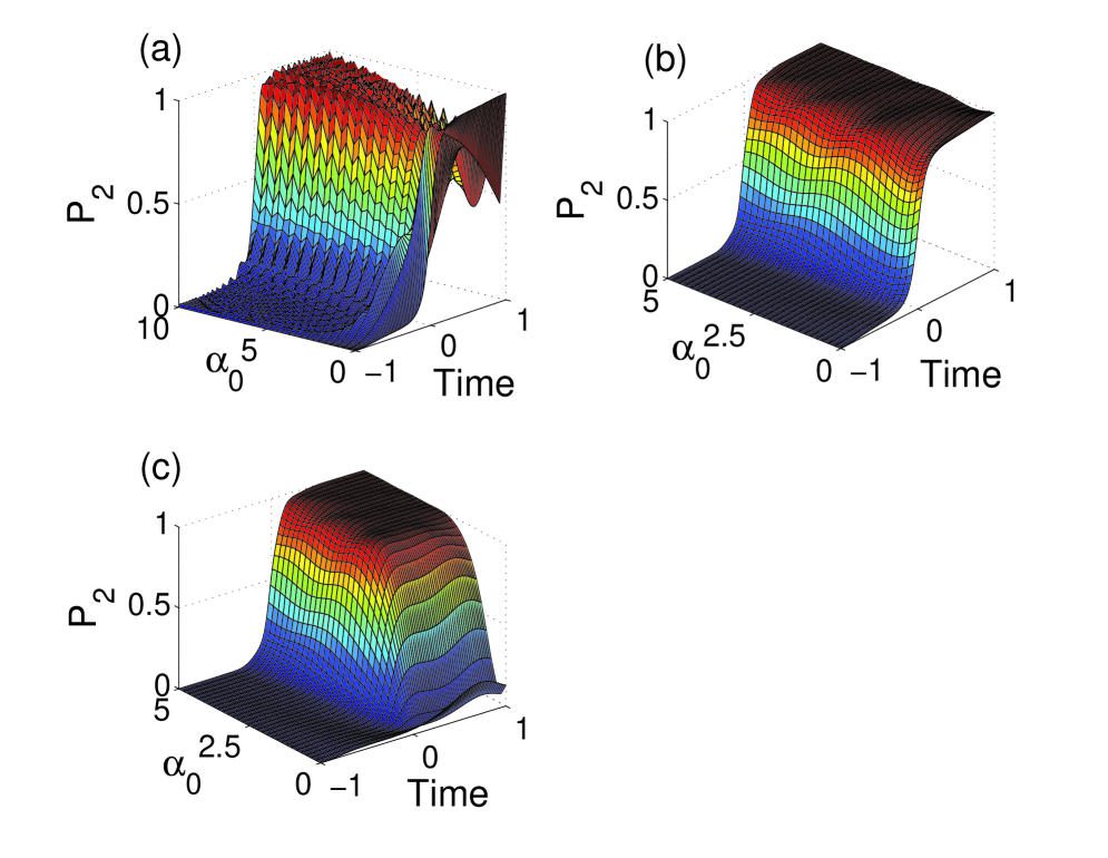
Figure 1: The time-dependent $P_{2}$ versus $\alpha_{0}$ (in units $\Omega_{0}$) when $\{\varphi=0,\ \zeta=3\Omega_{0},\ t_{f}=1/\Omega_{0}\}$: (a) $\alpha=\alpha_{0}$ is const; (b) $\alpha=\alpha_{0}\dot{\theta}$ is time-dependent. (c) $\alpha=\alpha_{0}\dot{\theta}$ is time-dependent and $\beta=0$. The evolution time in the figure is in units of $1/\Omega_{0}$.

Firstly, we discuss the situation when $\gamma=0$ (the system is Hermitian). In the interest of the effect of $\alpha$’s on STA, we set $\varphi=0$ in this part. Two kinds of $\alpha$ will be discussed by numerical simulation. (1): $\alpha$ is time-independent. Fig. 1 (a) shows the time-dependent population of the target state $|2\rangle$ ($P_{2}$) versus $\alpha$ when the initial state is $|1\rangle$ and $\{\varphi=0,\ \zeta=3\Omega_{0},\ t_{f}=1/\Omega_{0}$}. The result shows that in most of the cases, the shortcut could be constructed successfully and the populations could be transferred to the target state in a very short time. The oscillation is caused by the diagonal term in eq. (93). (2): $\alpha$ is time-dependent. For convenience, we choose $\alpha=\alpha_{0}\dot{\theta}$ ($\alpha_{0}$ is time-independent). As shown in Fig. 1 (b), a nearly perfect population transfer from $|1\rangle$ to $|2\rangle$ is realizable with arbitrary $\alpha_{0}$. What is more, according to eq. (93), it is obvious when $\alpha_{0}$ is large enough, $\alpha_{0}+i\approx\alpha_{0}$. This means, if we choose a relatively large $\alpha_{0}$, we can neglect the imaginary part of $A_{12}$ ($A_{21}$). This would make sense because a pulse with form of $\alpha_{0}\dot{\theta}$ would be more easily to realize than the form of $i\dot{\theta}$ in experiment. We plot Fig. 1 (c) which shows the result when $\beta=0$ (the other parameters are also $\{\varphi=0,\ \zeta=3\Omega_{0},\ t_{f}=1/\Omega_{0}$}). From the figure, we find the population transfer would be ideally achieved as long as $\alpha_{0}>2.5$.

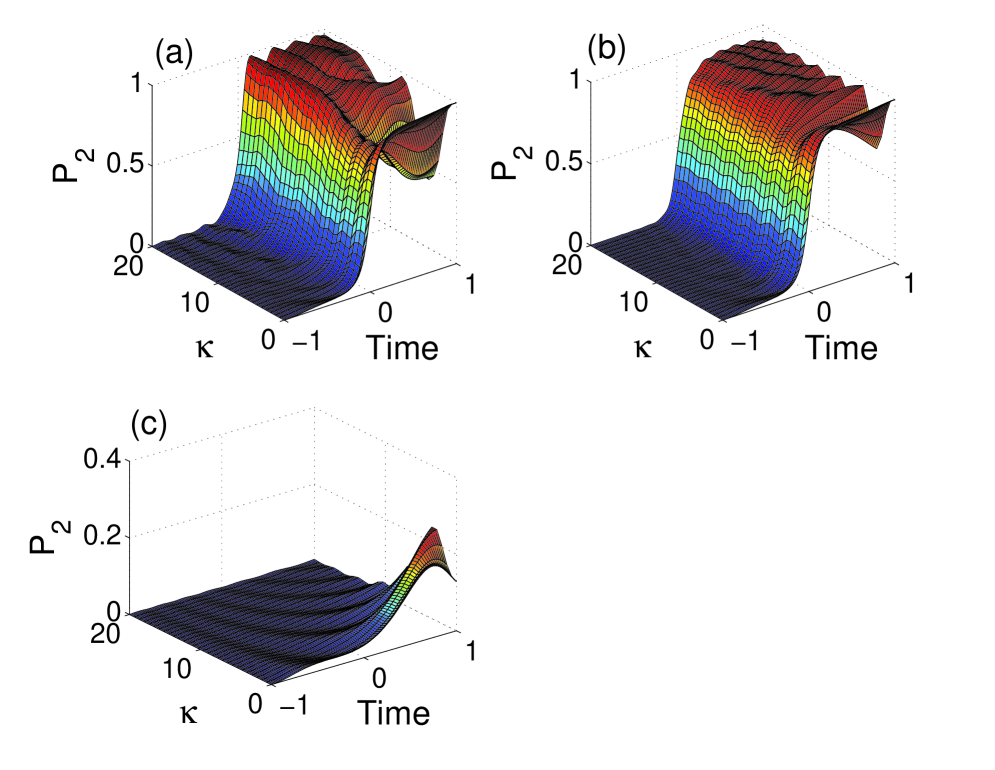
Figure 2: The time-dependent $P_{2}$ versus $\kappa$ (in units $\Omega_{0}$) when $\{\varphi=\kappa t,\ \zeta=3\Omega_{0},\ t_{f}=1/\Omega_{0}\}$: (a) based on the original transitionless tracking algorithm that $\alpha=-(\kappa/2)\sin{2\theta}$; (b) based on the present method with parameter $\alpha=0$; (c) based on $H_{0}$ without the adding term. The evolution time in the figure is in units of $1/\Omega_{0}$.

In the following, we will analyze the effectivity of the method when $\varphi\neq 0$. In Fig. 2 (a), we give $P_{2}$ versus $\kappa$ when the initial state is $|1\rangle$ and $\{\alpha=-\frac{\dot{\varphi}}{2}\sin{2\theta},\ \varphi=\kappa t,\ \zeta=3\Omega_{0}\}$. As shown in the figure, when $t=t_{f}$, while oscillating, the fidelity of the target state $|2\rangle$ increases with $\kappa$’s increasing. Which means if the adiabatic phase is considered, the effectivity of STA may reduce in some situation. For comparison, in Fig. 2 (b), we plot the time-evolution of state $|2\rangle$ versus $\kappa$ with $\{\alpha=0,\ \varphi=\kappa t,\ \zeta=3\Omega_{0}\}$. It is obvious that the second set of parameters behave better in restraining the adverse effect caused by $\varphi$ than the first set. The oscillation in Figs. 2 (a) and (b) is caused by the original Hamiltonian $H_{0}$ when $\Delta$ is large enough as shown in Fig. 2 (c). In addition, it is not hard to find that using the second set of parameters to construct shortcut can save more energy. According to eq. (93), the eigenvalue of $H_{add}$ is $E^{a}_{\pm}=\pm\hbar\sqrt{(\dot{\varphi}/2-\alpha\cot{2\theta})^{2}+\alpha^{2}+\dot{\theta}^{2}}$. This means the energy cost for constructing shortcuts is the least when $\alpha=0$.

In the following, we will briefly discuss the present method’s efficiency in the non-Hermitian system. Since the system is non-Hermitian, the dynamics of the system’s density operator $\rho(t)$ will be given as $\frac{d}{dt}{\rho(t)}=\frac{1}{i\hbar}[H(t)\rho(t)-\rho(t)H^{{\dagger}}(t)]$, where $H(t)=H_{0}(t)+H_{add}(t)$. First of all, we assume the population for a state $|j\rangle$ is still given as $P_{j}=|\langle j|\rho(t)|j\rangle|$, and display the populations $P_{1}$ and $P_{2}$ versus time in Fig. 3 with parameters $\{\alpha=0,\ \varphi=0,\ \zeta=3\Omega_{0},\gamma=0.5\Omega_{0}\}$. It should be noted here, since the Hamiltonian is non-Hermitian, if the population for a state is still given by $P_{j}=|\langle j|\rho(t)|j\rangle|$, the norm of the state vector given by $P_{1}+P_{2}$ will not be conserved during the evolution. This property can be seen in Fig. 3, where the norm is not conserved during the interaction. To avoid some problems caused by $P_{1}+P_{2}\neq 1$, some definitions of population in non-Hermitian system have been proposed Jpa45415201 ; Pra89033403 . However, since we only concern about the realizable possibility of the fast population inversion in the non-hermitian system, for simplicity, we define relative populations $P_{j}^{\prime}=P_{j}/(P_{j}+P_{k})$ ($j\neq k$) to help to analyze, and if no otherwise specified, $\alpha=0$, $\varphi=0$, and $\zeta=3\Omega_{0}$ will be used throughout the discussion in this part. In Fig. 4 we display the time-dependent relative populations for states $|1\rangle$ [Fig. 4 (a)] and $|2\rangle$ [Fig. 4 (b)] versus $\gamma$, where $\gamma$ is assumed time-independent. As we can see, the fast population inversion still could be achieved even with a relative large $\gamma$, i.e., $\gamma=\Omega_{0}$. As it is known, in general, $\gamma$ could also depend on time, $\gamma=\gamma(t)$, as an effective decay rate controlled by further interactions [see, e.g., ref. Jpb41175501 ]. According to the form of $\gamma$ in ref. Jpb41175501 , we plot Fig. 5 to show that the present method can also work very well in the case of $\gamma$ is time-dependent, which shows the populations versus time with the parameters mentioned above. Fig. 5 (b) shows the relative populations versus time, and $\gamma$ is chosen as $\gamma=\frac{1}{2+t^{2}}$ for simplicity in plotting the figures. Moreover, if $\gamma$ is controllable, or if $\gamma$ could satisfy some kind of function, for example, $\gamma=\pm\dot{\theta}/\sin{2\theta}$, the scheme can make the population transfer fast without increasing the coupling Pra86033813 because when $\gamma=\pm\dot{\theta}/\sin{2\theta}$, the corresponding $\beta=0$. Such assumption can be physically realized, for instance, in two coupled optical waveguides with longitudinally varying gain and loss regions Pra86033813 . In fact, $\gamma=\pm\dot{\theta}/\sin{2\theta}$ is just the result of ref. Pra8705250289063412 which has been analyzed and discussed in very detail.

From the analysis above, we find the real part of pulse Re$A_{12}$ could be arbitrary time-dependent function, which means the real part is obviously realizable. So, to make sure the pulses we used in the schemes are realizable, we need to confirm that whether the imaginary part of the pulse is realizable or not. Fig. 6 shows Im$A_{12}$ versus time with different parameters when $\varphi=0$. Shown in the figure, the shapes are all similar to Gaussian curves, which means the pulses are not hard to be realized in practice. In other words, the schemes proposed in the paper are feasible in practice.

In conclusion, we have proposed a different and flexible way to design the adding Hamiltonian for the original Hamiltonian to construct shortcuts to adiabaticity (STA). The method maybe promising to avoid the trouble (the speed-up protocols’ Hamiltonian may involve the terms which are difficult to be realized in practice) because of the multiple-choices of the adding Hamiltonian. We have applied this method to the Landau-Zener model as an application example, and the results show the method works very well in two-level systems (in both Hermitian and non-Hermitian). In Hermitian system, we find a relatively suitable $\alpha$ (the real part of the off-diagonal terms in the adding Hamiltonian), we can even speed up the adiabatic process without the imaginary part of the off-diagonal terms in the adding Hamiltonian. That is meaningful because amending the Rabi frequency $\Omega$ by real correction will be much more easily than by imaginary correction. In non-Hermitian system, different from ref. Pra8705250289063412 where $\gamma$ (gain or loss of population) nullifies the counterdiabatic coupling to speed up the adiabatic evolution all alone, in this paper, $\gamma$ cooperates with $\beta$ (the correction of the imaginary part of Rabi frequency) to achieve the goals. As is known, the decay $\gamma$ is usually decided by the system and is uncontrollable, so a speed-up protocol with a fixed form of $\gamma$ will be hard to realize and generalize. However, in our present method, the correction of Rabi frequency $\beta$ cooperates with $\gamma$ to construct shortcuts, hence, as long as the corresponding $\beta$ is realizable in practice, the shortcuts could be constructed with arbitrary $\gamma$. Another highlight of this method is that the phase change at any time could be obviously calculated which may have application prospect in quantum phase gates.

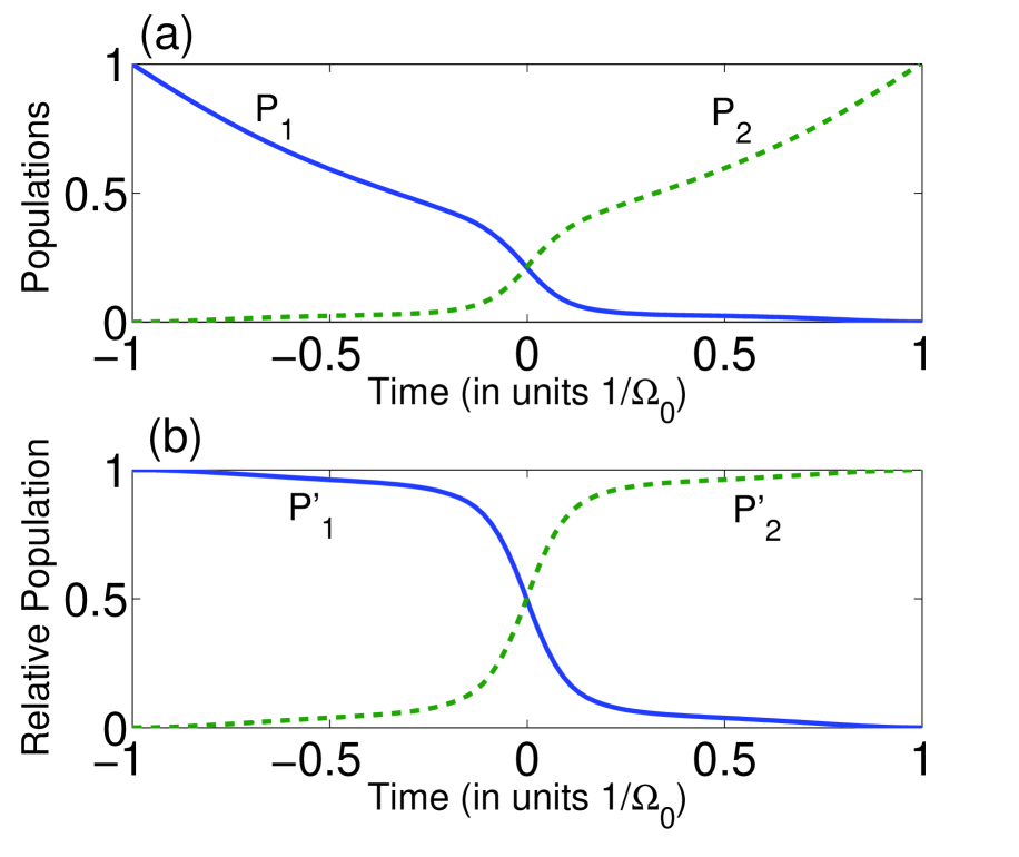
Figure 3: (a) The populations $P_{1}$ and $P_{2}$ versus time when $\gamma=0.5\Omega_{0}$. (b) The relative population $P^{\prime}_{1}$ and $P^{\prime}_{2}$ versus time when $\gamma=0.5\Omega_{0}$.

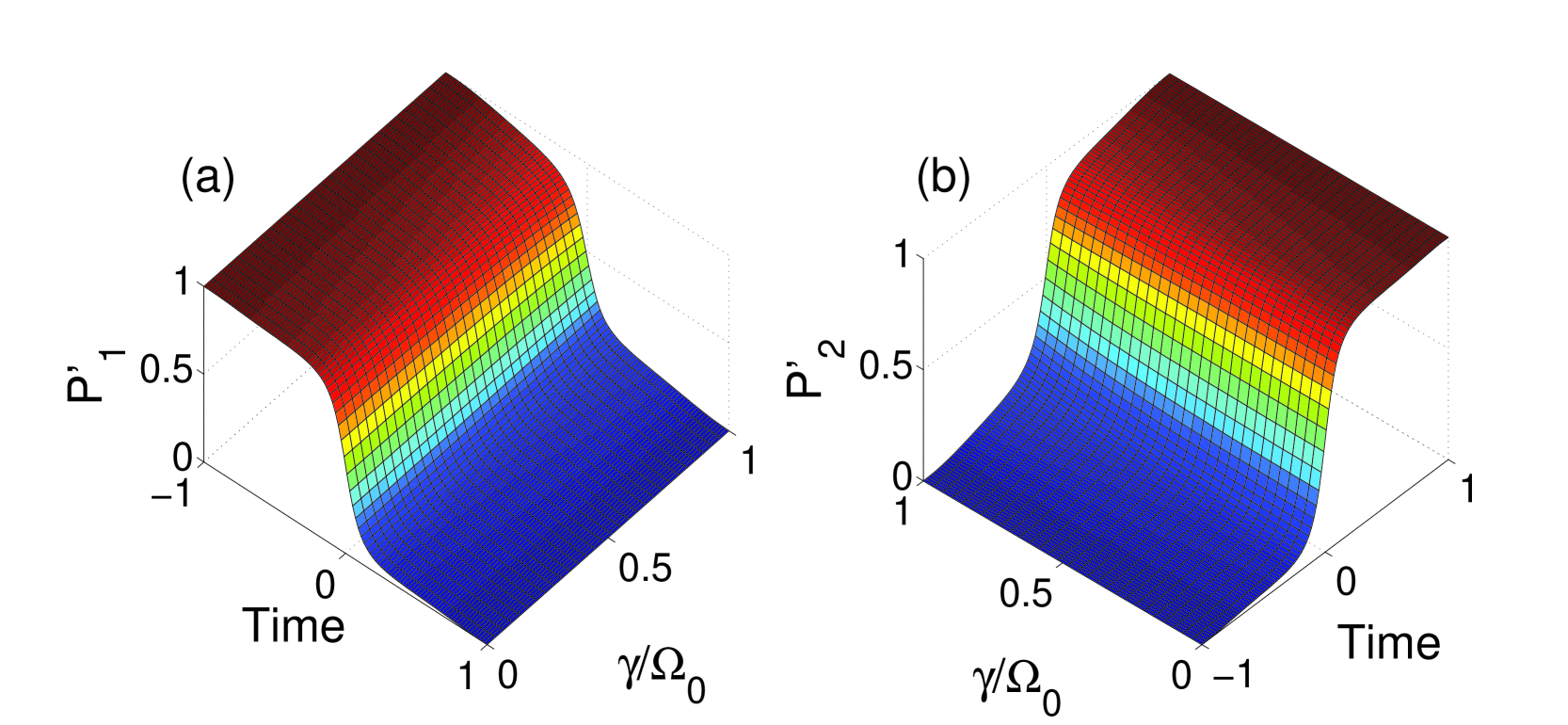
Figure 4: (a) The time-dependent relative population $P^{\prime}_{1}$ versus $\gamma$. (b) The time-dependent relative population $P^{\prime}_{2}$ versus $\gamma$. The evolution time in the figure is in units of $1/\Omega_{0}$.

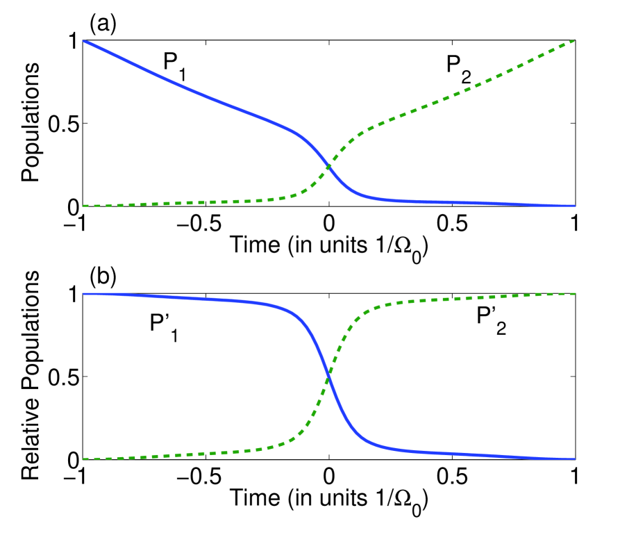
Figure 5: (a) The populations $P_{1}$ and $P_{2}$ versus time when $\gamma=1/(2+t^{2})$. (b) The relative population $P^{\prime}_{1}$ and $P^{\prime}_{2}$ versus time when $\gamma=1/(2+t^{2})$.

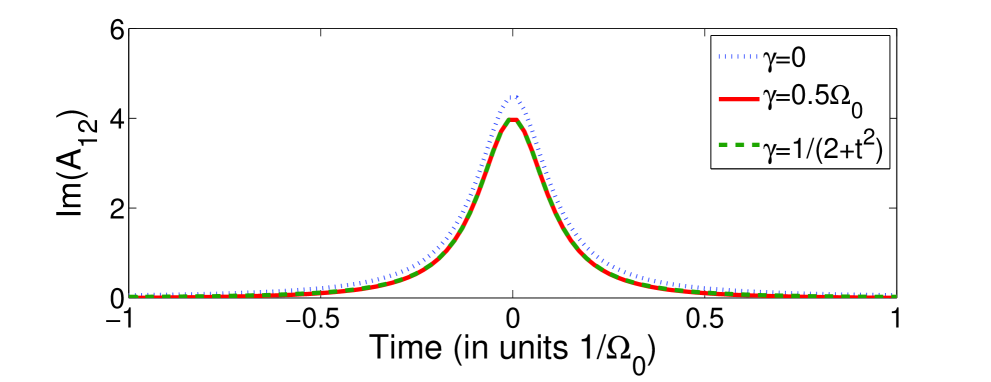
Figure 6: The shapes of the imaginary part of the adding Hamiltonian’s pulses when $\varphi=0$. Blue dotted curve when $\gamma=0$; Red solid curve when $\gamma=0.5\Omega_{0}$; Green dashed curve when $\gamma=1/(2+t^{2})$.

References

(1) M. Demirplak and S. A. Rice,
J. Phys. Chem. A
107, 9937 (2003);
J. Chem. Phys.
129, 154111 (2008).
(2) M. B. Berry,
J. Phys. A
42, 365303 (2009).
(3) X. Chen, I. Lizuain, A. Ruschhaupt, D. Guéry-Odelin, and J. G. Muga,
Phys. Rev. Lett.
105, 123003 (2010).
(4) E. Torrontegui, S. Ibáñez, S. Martínez-Garaot, M. Modugno, A. del Campo, D. Gué-Odelin, A. Ruschhaupt,
X. Chen, and J. G. Muga,
Adv. Atom. Mol. Opt. Phys.
62, 117 (2013).
(5) A. del Campo,
Phys. Rev. Lett.
111, 100502 (2013).
(6) X. Chen, E. Torrontegui, and J. G. Muga,
Phys. Rev. A
83, 062116 (2011).
(7) X. Chen and J. G. Muga,
Phys. Rev. A
86, 033405 (2012).
(8) E. Torrontegui, S. Ibáñez, X. Chen, A. Ruschhaupt, D. Guéry-Odelin, and J. G. Muga,
Phys. Rev. A
83, 013415 (2011).
(9) J. G. Muga, X. Chen, S. Ibáñez, I. Lizuain, and A. Ruschhaupt,
J. Phys. B
43, 085509 (2010).
(10) E. Torrontegui, Xi Chen, M. Modugno, A. Ruschhaupt, D. Guéry-Odelin, and J. G. Muga,
Phys. Rev. A
85, 033605 (2012).
(11) S. Masuda, and K. Nakamura,
Phys. Rev. A
84, 043434 (2011).
(12) M. Lu, Y. Xia, L. T. Shen, J. Song, and N. B. An,
Phys. Rev. A
89, 012326 (2014).
(13) M. Lu, Y. Xia, L. T. Shen, and J. Song,
Laser Phys.
24, 105201 (2014).
(14) Y. H. Chen, Y. Xia, Q. Q. Chen, and J. Song,
Phys. Rev. A
89, 033856 (2014); 91, 012325 (2015);
Laser Phys. Lett.
11, 115201 (2014);
Sci. Rep.
5, 15616 (2015).
(15) J. G. Muga, X. Chen, A. Ruschhaup, and D. Guéry-Odelin,
J. Phys. B
42, 241001 (2009).
(16) X. Chen, A. Ruschhaupt, S. Schmidt, A. del Campo, D. Guéry-Odelin, and J. G. Muga
Phys. Rev. Lett.
104, 063002 (2010).
(17) X. Chen and J. G. Muga,
Phys. Rev. A
82, 053403 (2010).
(18) J. F. Schaff, P. Capuzzi, G. Labeyrie, and P. Vignolo,
New J. Phys.
13, 113017 (2011).
(19) X. Chen, E. Torrontegui, D. Stefanatos, J. S. Li, and J. G. Muga,
Phys. Rev. A
84, 043415 (2011).
(20) E. Torrontegui, X. Chen, M. Modugno, S. Schmidt, A. Ruschhaupt, and J. G. Muga,
New J. Phys.
14, 013031 (2012).
(21) A. del Campo,
Phys. Rev. A
84, 031606(R) (2011);
Eur. Phys. Lett.
96, 60005 (2011).
(22) A. Ruschhaupt, X Chen, D. Alonso, and J. G. Muga,
New J. Phys.
14, 093040 (2012).
(23) J. F. Schaff, X. L. Song, P. Vignolo, and G. Labeyrie,
Phys. Rev. A
82, 033430 (2010).
(24) J. F. Schaff, X. L. Song, P. Capuzzi, P. Vignolo, and G. Labeyrie,
Eur. Phys. Lett.
93, 23001 (2011).
(25) S. Ibáñez, X. Chen, E. Torrontegui, J. G. Muga, and A. Ruschhaupt,
Phys. Rev. Lett.
109, 100403 (2012).
(26) S. Martínez-Garaot, E. Torrontegui, X. Chen, and J. G. Muga,
Phys. Rev. A
89, 053408 (2014).
(27) T. Opatrný and K. Mølmer,
New J. Phys.
16, 015025 (2014).
(28) H. Saberi, T. Opatrny, K. Mølmer, and A. del Campo,
Phys. Rev. A
90, 060301(R) (2014).
(29) S. Ibáñez, X. Chen, and J. G. Muga,
Phys. Rev. A
87, 043402 (2013).
(30) E. Torrontegui, S. Martínez-Garaot, and J. G. Muga,
Phys. Rev. A
89, 043408 (2014).
(31) B. T. Torosov, G. Della Valle, and S. Longhi,
Phys. Rev. A
87, 052502 (2013);
89, 063412 (2014).
(32) S. Ibáñez, S. Martínez-Garaot, X. Chen, E. Torrontegui, and J. G. Muga,
Phys. Rev. A
84, 023415 (2011).
(33) E. M. Graefe and H. J. Korsch,
Czech. J. Phys.
56, 1007 (2006).
(34) S. A. Reyes, F. A. Olivares, and L. Morales-Molina,
J. Phys. A
45, 444027 (2012).
(35) R. El-Ganainy, K. G. Makris, and D. N. Christodoulides,
Phys. Rev. A
86, 033813 (2012).
(36) N. Moiseyev,
Phys. Rev. A
83, 052125 (2011).
(37) A. Leclerc, D. Viennot, and G. Jolicard,
J. Phys. A
45, 415201 (2012).
(38) S. Ibáñez and J. G. Muga,
Phys. Rev. A
89, 033403 (2014).
(39) J. G. Muga, J. Echanobe, A. del Campo, and I. Lizuain,
J. Phys. B
41, 175501 (2008).