Octupole correlations in low-lying states of ¹⁵⁰Nd and ¹⁵⁰Sm and their impact on neutrinoless double-beta decay

Abstract

We present a generator-coordinate calculation, based on a relativistic energy-density functional, of the low-lying spectra in the isotopes ¹⁵⁰Nd and ¹⁵⁰Sm and of the nuclear matrix element that governs the neutrinoless double-beta decay of the first isotope to the second. We carefully examine the impact of octupole correlations on both nuclear structure and the double-beta decay matrix element. Octupole correlations turn out to reduce quadrupole collectivity in both nuclei. Shape fluctuations, however, dilute the effects of octupole deformation on the double-beta decay matrix element, so that the overall octupole-induced quenching is only about 7%.

I Introduction

The nucleus ¹⁵⁰Nd has been the active isotope in double-beta ($\beta\beta$) decay experiments Argyriades et al. (2009), and may be again in the future Bongrand (2015). It has $N=90$ neutrons and is part of a set of isotones in which nuclear structure changes rapidly as neutrons are added or removed. Ref. Casten and Zamfir (2001) showed that the low-lying states of ¹⁵⁰Nd and other $N=90$ isotones are close to the predictions of the X(5) model, which describes the critical point of a first order phase transition from spherical harmonic vibrator to axially-deformed rotor. A significant amount of work on nuclear phase transitions in the $N\simeq 90$ isotones followed this discovery Krücken et al. (2002); Meng et al. (2005); Sheng and Guo (2005); Nikšić et al. (2007); Rodríguez-Guzmán and Sarriguren (2007); Rodriguez and Egido (2008); Robledo et al. (2008); Li et al. (2009). We concern ourselves here, however, with a different aspect of structure in ¹⁵⁰Nd: octupole correlations, suggested by the observation of low-lying negative-parity states and fast $E3$ transitions Urban et al. (1987); Friedrichs et al. (1992); Bvumbi et al. (2013). Refs. Nazarewicz and Tabor (1992); Garrote et al. (1998); Babilon et al. (2005); Minkov et al. (2006); Zhang et al. (2010); Robledo and Bertsch (2011); Rodríguez-Guzmán et al. (2012) applied a wide variety of models with octupole shape degrees of freedom to nuclei with $N\simeq 90$. The models indicated that the proton 1h_11/2–2d_5/2 and neutron 1i_13/2–2f_7/2 orbitals near the Fermi levels are responsible for the strong octupole correlations. And very recently the authors of Refs. Nomura et al. (2014, 2015) used the $sdf$ interacting Boson model (IBM), with Hamiltonian parameters determined from self-consistent mean-field calculations, to successfully describe the low-lying states of $N\simeq 90$ nuclei. These studies imply that the low-lying states of ¹⁵⁰Nd are dominated by the quadrupole-octupole collective excitations and that the EDF approaches provide good basis states for them.

The $sdf$ IBM calculation Nomura et al. (2014, 2015) can be regarded — very roughly speaking — as something like an EDF-based shell-model calculation with the model space truncated to states constructed from nucleon pairs with angular momentum $J=0,2$, and 3. It obviously contains correlations beyond those of mean-field theory. In this paper, we carry out a symmetry-projected beyond-mean-field calculation, using the Generator Coordinate Method (GCM) to study the low-lying states of ¹⁵⁰Nd and ¹⁵⁰Sm and to quantify the effects of octupole correlations on the matrix element that governs neutrinoless double-beta ($0\nu\beta\beta$) decay from the ground state of the first to that of the second. Our starting point is a self-consistent relativistic mean-field (RMF) calculation Reinhard (1989); Ring (1996); Vretenar et al. (2005); Meng et al. (2006) with constraints on both quadrupole and octupole mass moments, part of a framework that has already been used to study static octupole deformation in nuclear ground states Geng et al. (2007); Guo et al. (2010); Zhang et al. (2010); Lu et al. (2012); Li et al. (2013). The GCM approach we take here (also known as multi-reference covariant density-functional theory) allows us to go beyond mean-field theory, however, by including dynamical correlations associated with symmetry restoration and shape fluctuations Nikšić et al. (2006); Yao et al. (2013); Wu et al. (2014); Wu and Zhou (2015); Yao et al. (2010, 2011, 2014). Octupole shape fluctuations Yao et al. (2015a); Zhou et al. (2016) have not yet been studied extensively. Previous work on the $\beta\beta$ decay of ¹⁵⁰Nd has shown that the matrix elements are sensitive to quadrupole deformation Hirsch et al. (1995); Chaturvedi et al. (2008); Fang et al. (2010); Rodríguez and Martinez-Pinedo (2010); Mustonen and Engel (2013); Song et al. (2014); Terasaki (2015); Yao et al. (2015b). It is the effect of octupole correlations that we address here.

This paper is organized as follows: Section II briefly presents the RMF theory that we use to generate reference states, the GCM and several projection techniques that we apply to nuclear collective quadrupole and octupole excitations, and the formulae for computing the matrix elements of the operator responsible for $0\nu\beta\beta$ decay. Section III presents our results for the structure of low-lying states in ¹⁵⁰Nd and ¹⁵⁰Sm, and for the $0\nu\beta\beta$ matrix elements, which we compare with those of previous studies that neglect octupole degrees of freedom. Section IV summarizes our findings.

II The model

II.1 Generating mean-field reference states in collective coordinate space

The first step in the GCM procedure is to generate a set of collective reference (or basis) states $|q\rangle$. We do so by carrying out constrained mean-field calculations based with a relativistic point-coupling energy-density functional (EDF) Nikolaus et al. (1992); Bürvenich et al. (2002); Zhao et al. (2010):

$${{E}}_{\textnormal{RMF}}=\int d{\bm{r}}~{}{\mathcal{E}_{\textnormal{RMF}}}[\rho,j]\,,$$ (1)

where $\mathcal{E}_{\rm RMF}$ is defined as

$${\mathcal{E}_{\textnormal{RMF}}}[\rho,j] =\sum_{k,\tau}v_{k,\tau}^{2}\,{\bar{\psi}_{k,\tau}(\bm{r})\left(-i\bm{\gamma}\bm{\nabla}+m\right)\psi_{k,\tau}(\bm{r})}$$

$$+\frac{\alpha_{0}}{2}\rho^{2}+\frac{\beta_{0}}{3}\rho^{3}+\frac{\gamma_{0}}{4}\rho^{4}+\frac{\delta_{0}}{2}\rho\triangle\rho$$

$$+\frac{\alpha_{1}}{2}j_{\mu}j^{\mu}+\frac{\gamma_{1}}{4}(j_{\mu}j^{\mu})^{2}+\frac{\alpha_{11}}{2}\tilde{j}^{\mu}\tilde{j}_{\mu}$$

$$+\frac{\delta_{1}}{2}j_{\mu}\triangle j^{\mu}+\frac{\delta_{11}}{2}\tilde{j}^{\mu}\triangle\tilde{j}_{\mu}$$

$$+\frac{\alpha_{10}}{2}\tilde{\rho}^{2}+\frac{\delta_{10}}{2}\tilde{\rho}\triangle\tilde{\rho}+\frac{1}{4}e(j_{\mu}-\tilde{j}_{\mu})A^{\mu}\,.$$ (2)

Here $\tau=1$ (neutron) or $-1$ (proton), $\psi_{k,\tau}$ is the Dirac wave function for the $k^{\rm th}$ nucleon with isospin $\tau$, and $A^{\mu}$ is the electromagnetic field. The functional contains eleven constants $\alpha$, $\beta$, $\gamma$ and $\delta$. The local isoscalar and isovector densities $\rho$ and $\tilde{\rho}$, and the corresponding isoscalar and isovector currents $j_{\mu}$ and $\tilde{j}_{\mu}$ are

$$\rho({\bm{r}}) =\sum_{k,\tau}v_{k,\tau}^{2}\,\bar{\psi}_{k,\tau}({\bm{r}})\psi_{k,\tau}({\bm{r}})\,,$$ (3a)

$$\tilde{\rho}({\bm{r}}) =\sum_{k,\tau}\tau\,v_{k,\tau}^{2}~{}\bar{\psi}_{k,\tau}({\bm{r}})\psi_{k,\tau^{\prime}}({\bm{r}})\,,$$ (3b)

$$j^{\mu}({\bm{r}}) =\sum_{k,\tau}v_{k,\tau}^{2}~{}\bar{\psi}_{k,\tau}({\bm{r}})\gamma^{\mu}\psi_{k,\tau}({\bm{r}})\,,$$ (3c)

$$\tilde{j^{\mu}}({\bm{r}}) =\sum_{k,\tau}\tau\,v_{k,\tau}^{2}\,\bar{\psi}_{k,\tau}({\bm{r}})\gamma^{\mu}\psi_{k,\tau}({\bm{r}})\,.$$ (3d)

These quantities are calculated in the no-sea approximation, i.e. with the summation in Eqs. (3a) – (3d) running over all states with $v^{2}_{k,\tau}>0$, where the $v_{k,\tau}^{2}$ is the occupation probability for the $k^{\rm th}$ nucleon of type $\tau$ in the BCS wave function

$$|q\rangle=\prod_{k>0,\tau}(u_{k,\tau}+v_{k,\tau}c^{\dagger}_{k,\tau}c^{\dagger}_{\bar{k},\tau})|0\rangle\,.$$ (4)

The numbers $u_{k,\tau}$ and $v_{k,\tau}$ obey $u^{2}_{k,\tau}+v^{2}_{k,\tau}=1$. The operator $c^{\dagger}_{k,\tau}$ creates a nucleon of type $\tau$ in the single-nucleon state $k$. The corresponding spinor $\psi_{k,\tau}$ is determined by the variational principle

$$\delta\langle q|\hat{H}-\sum_{\tau}\lambda_{\tau}\hat{N}_{\tau}-\sum_{\lambda=1,2,3}C_{\lambda}(\hat{Q}_{\lambda 0}-q_{\lambda})^{2}|q\rangle=0\,,$$ (5)

with the Lagrange multipliers $\lambda_{\tau}$ fixed by the constraints $\langle q|\hat{N}_{1}|q\rangle=N$ and $\langle q|\hat{N}_{-1}|q\rangle=Z$. The deformation parameters $\beta_{\lambda}$ ($\lambda=2,3$) are related to the mass multipole moments by

$$\beta_{\lambda}\equiv\dfrac{4\pi}{3AR^{\lambda}}q_{\lambda},\quad R=1.2A^{1/3}\,,$$ (6)

with $A$ representing the mass number of the nucleus under consideration.

We iteratively solve the Dirac equation derived from (5) by expanding the Dirac spinors $\psi_{k,\tau}$ in a basis of single-particle oscillator states within 12 shells Gambhir et al. (1990). As Eq. (4) indicates, we treat pairing correlations in the BCS approximation, with a density-independent zero-range pairing interaction Krieger et al. (1990). We always employ the relativistic energy density functional PC-PK1 Zhao et al. (2010). Previous symmetry-projected GCM studies Nikšić et al. (2007); Song et al. (2014) have shown that the low-lying states produced by the PC-PK1 and the PC-F1 Bürvenich et al. (2002) are close to each other in energy, suggesting that reasonable changes in the particle-hole structure of the energy-density functional will not produce major changes in low-lying structure. The pairing functional, however, has been shown to have a significant effect in ¹⁵⁰Nd, on both in its collective structure Li et al. (2011) and its matrix element for neutrinoless double beta decay Song et al. (2014). Here, as in Ref. Song et al. (2014) we choose to fit the pairing strengths to the average pairing gaps produced by a separable finite-range pairing force at the mean-field energy minimum Tian et al. (2009). The procedure leads to pairing gaps that are similar to those obtained both from the Gogny functional and experiment.

II.2 Symmetry restoration and configuration mixing

We construct physical state vectors $|J^{\pi}_{\alpha}\rangle$ by superposing projected mean-field reference states:

$$|J^{\pi}_{\alpha}\rangle=\sum_{q}f^{J\pi\alpha}_{q}|JM\pi NZ;q\rangle\,,$$ (7)

where $|JM\pi NZ;q\rangle\equiv\hat{P}^{J}_{M0}\hat{P}^{N}\hat{P}^{Z}\hat{P}^{\pi}|q\rangle$, with the “0” in the first projector corresponding to the intrinsic quantum number $K$ (which will be zero for all our states) and the collective coordinate $q$ standing for the intrinsic deformation parameters $(\beta_{2},\beta_{3})$ of the reference states. The $\hat{P}$’s are projection operators onto states with well-defined angular momentum $J$ and its $z$-component $M$, parity ($\pi=\pm$), and neutron and proton number ($N,Z$) Ring and Schuck (1980). [$N$, $Z$, and $K$ are implied on the left-hand side of Eq. (7)]. The weight functions $f^{J\pi\alpha}_{q}$, where $\alpha$ is a simple enumeration index, are solutions to the Hill-Wheeler-Griffin equation Hill and Wheeler (1953); Griffin and Wheeler (1957)

$$\sum_{q^{\prime}}\left[\mathscr{H}^{J\pi}_{q,q^{\prime}}-E^{J\pi}_{\alpha}\mathscr{N}^{J\pi}_{q,q^{\prime}}\right]f^{J\pi\alpha}_{q^{\prime}}=0\,,$$ (8)

where the Hamiltonian kernel $\mathscr{H}^{J\pi}_{q,q^{\prime}}$ and the norm kernel $\mathscr{N}^{J\pi}_{q,q^{\prime}}$ are given by

$$\left\{\begin{array}[]{c}\mathscr{H}\\ \mathscr{N}\end{array}\right\}^{J\pi}_{q,q^{\prime}}=\langle q|\left\{\begin{array}[]{c}\hat{H}\\ 1\end{array}\right\}\hat{P}^{J}_{00}\hat{P}^{N}\hat{P}^{Z}\hat{P}^{\pi}|q^{\prime}\rangle\,,$$ (9)

To solve Eq. (8), we first diagonalize the norm kernel $\mathscr{N}$ and then use the non-zero eigenvalues and corresponding eigenvectors to construct the “natural basis” Ring and Schuck (1980); Rodriguez-Guzman et al. (2002); Yao et al. (2010). We re-diagonalize the Hamiltonian in that basis to obtain the states $|J^{\pi}_{\alpha}\rangle$ and the energies $E^{J\pi}_{\alpha}$.

Because we begin with an energy functional rather than a Hamiltonian, we need a prescription for the off-diagonal matrix elements of $\mathscr{H}$. Following standard practice, we simply replace the diagonal density in the functional by the transition density. Though the prescription brings with it spurious divergences and “steps” Lacroix et al. (2009); Duguet et al. (2009), it does not produce an unresolvable ambiguity when used together with the relativistic EDF in Eq. (1), which contains only integer powers of the density. We exclude exchange terms but avoid numerical instabilities in particle-number projection at the gauge angle $\phi=\pi/2$ by setting $L$ to 9 in Fomenko’s expansion Fomenko (1970). Refs. Rodriguez-Guzman et al. (2002); Nikšić et al. (2006); Bender and Heenen (2008); Rodríguez and Egido (2010); Yao et al. (2010) contain detailed discussions of beyond-mean-field calculations with energy-density functionals.

II.3 Nuclear matrix element for $0\nu\beta\beta$ decay

The $0\nu\beta\beta$ decay nuclear matrix element is

$$M^{0\nu} = \dfrac{4\pi R}{g^{2}_{A}(0)}\int\int d^{3}x_{1}d^{3}x_{2}\int\frac{d^{3}q}{(2\pi)^{3}}\frac{\text{e}^{\text{i}\bm{q}\cdot(\bm{x}_{1}-\bm{x}_{2})}}{q}$$ (10)

$$\times \sum_{m}\frac{\langle 0^{+}_{F}|\mathcal{J}_{\mu}^{\dagger}(\bm{x}_{1})|m\rangle\langle m|\mathcal{J}^{\mu\dagger}(\bm{x}_{2})|0^{+}_{I}\rangle}{q+E_{m}-(E_{I}+E_{F})/2},$$

where ${\cal J}^{\dagger}_{\mu}$ is the charge-changing nuclear current operator Avignone et al. (2008) and $q$ is the momentum transferred from leptons to nucleons. The nuclear radius $R=1.2A^{1/3}$ makes the matrix element dimensionless. In the closure approximation and with the GCM state vectors from Eq. (7) as ground states $|0^{+}_{I/F}\rangle$ of the initial and final nuclei, we obtain

$$M^{0\nu}=\sum_{q_{I},q_{F}}f^{0^{+}_{I}}_{q_{I}}f^{0^{+}_{F}}_{q_{F}}\langle q_{F}|\hat{\cal O}^{0\nu}\hat{P}^{J=0}_{00}\hat{P}^{N}\hat{P}^{Z}\hat{P}^{\pi=+}|q_{I}\rangle\,,$$ (11)

with the transition operator given by

$$\hat{\cal O}^{0\nu} = \dfrac{4\pi R}{g^{2}_{A}(0)}\int\frac{d^{3}q}{(2\pi)^{3}}\int\int d^{3}x_{1}d^{3}x_{2}\frac{\text{e}^{\text{i}\bm{q}\cdot(\bm{x}_{1}-\bm{x}_{2})}}{q(q+E_{d})}$$ (12)

$$\times [\mathcal{J}_{\mu}^{\dagger}(\bm{x}_{1})\mathcal{J}^{\mu\dagger}(\bm{x}_{2})]\,,$$

and $E_{d}$ set to $1.12A^{1/2}\simeq 13.72$ Mev Haxton and Stephenson (1984).

The operator $[\mathcal{J}_{\mu}^{\dagger}(\bm{x}_{1})\mathcal{J}^{\mu\dagger}(\bm{x}_{2})]$, when Fourier transformed, contains the terms Song et al. (2014),

$$VV: g_{V}^{2}(\bm{q}^{2})\left(\bar{\psi}\gamma_{\mu}\tau_{-}\psi\right)^{(1)}\left(\bar{\psi}\gamma^{\mu}\tau_{-}\psi\right)^{(2)}$$ (13)

$$AA: g_{A}^{2}(\bm{q}^{2})\left(\bar{\psi}\gamma_{\mu}\gamma_{5}\tau_{-}\psi\right)^{(1)}\left(\bar{\psi}\gamma^{\mu}\gamma_{5}\tau_{-}\psi\right)^{(2)}$$

$$AP: 2g_{A}(\bm{q}^{2})g_{P}(\bm{q}^{2})\left(\bar{\psi}\bm{\gamma}\gamma_{5}\tau_{-}\psi\right)^{(1)}\left(\bar{\psi}\bm{q}\gamma_{5}\tau_{-}\psi\right)^{(2)}$$

$$PP: g_{P}^{2}(\bm{q}^{2})\left(\bar{\psi}\bm{q}\gamma_{5}\tau_{-}\psi\right)^{(1)}\left(\bar{\psi}\bm{q}\gamma_{5}\tau_{-}\psi\right)^{(2)}$$

$$MM: g_{M}^{2}(\bm{q}^{2})\left(\bar{\psi}\frac{\sigma_{\mu i}}{2m_{N}}q^{i}\tau_{-}\psi\right)^{(1)}\left(\bar{\psi}\frac{\sigma^{\mu j}}{2m_{N}}q_{j}\tau_{-}\psi\right)^{(2)}\,,$$

where $\tau_{-}$ is the isospin lowering operator that changes neutrons into protons, $\sigma_{\mu\nu}=\frac{\text{i}}{2}\left[\gamma_{\mu},\gamma_{\nu}\right]$, and $V,A,P,M$ denote the vector, axial vector, pseudoscalar, and magnetic pieces of the one-nucleon current. Following Ref. Šimkovic et al. (1999), we take the form factors $g_{V}(\bm{q}^{2})$, $g_{A}(\bm{q}^{2})$, $g_{M}(\bm{q}^{2}),$ and $g_{P}(\bm{q}^{2})$ to be

$$g_{V}({\mathbf{q}}^{2}) = \dfrac{g_{V}(0)}{(1+{\mathbf{q}}^{2}/\Lambda^{2}_{V})^{2}},$$ (14a)

$$g_{A}({\mathbf{q}}^{2}) = \dfrac{g_{A}(0)}{(1+{\mathbf{q}}^{2}/\Lambda^{2}_{A})^{2}},$$ (14b)

$$g_{P}({\mathbf{q}}^{2}) = g_{A}({\mathbf{q}}^{2})\dfrac{2m_{N}}{{\mathbf{q}}^{2}+m^{2}_{\pi}}(1-\dfrac{m^{2}_{\pi}}{\Lambda^{2}_{A}}),$$ (14c)

$$g_{M}({\mathbf{q}}^{2}) = (\mu_{p}-\mu_{n})g_{V}({\mathbf{q}}^{2}),$$ (14d)

with $g_{V}(0)=1.0$, $g_{A}(0)=1.254$, $\mu_{p}-\mu_{n}=3.70$, $\Lambda^{2}_{V}=0.710$ (GeV)², $\Lambda_{A}=1.09$ GeV, $m_{N}=0.93827$ GeV and $m_{\pi}=0.13957$ GeV. For the sake of simplicity, we neglect short-range correlations.

We include, alongside the generator coordinates from Ref. Song et al. (2014), the octupole deformation parameter $\beta_{3}$. The parity breaking (and subsequent projection) and the larger number of reference states caused by the inclusion of octupole deformation increase computing time but otherwise cause no problems in our calculation. We initially include 50 reference states with $\beta_{3}>0$. From this set, 29 natural states turn out to sufficient to include essentially all the contributions of the original 50 states to both structure properties and $0\nu\beta\beta$ decay matrix elements.

III Results and discussion

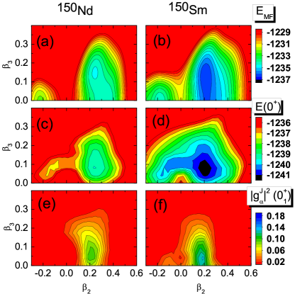
Figure 1: (Color online) Mean-field energy surfaces for ¹⁵⁰Nd (a) and ¹⁵⁰Sm (b), projected energy surfaces for ¹⁵⁰Nd (c) and ¹⁵⁰Sm (d), and the square of the collective ground-state wave function for ¹⁵⁰Nd (e) and ¹⁵⁰Sm (f), all in the $\beta_{2}$-$\beta_{3}$ plane.

Figure 1 shows the mean-field and quantum-number-projected energy surfaces, as well as the collective wave functions $|g^{J}_{\alpha}(q)|^{2}$, for the ground states of ¹⁵⁰Nd and ¹⁵⁰Sm. The collective wave functions, defined as $g^{J\pi}_{\alpha}(q)\equiv\sum_{q^{\prime}}\left[\mathscr{N}^{J\pi}_{q,q^{\prime}}\right]^{1/2}f^{J\pi\alpha}_{q^{\prime}}$, provide information about the importance of deformation in the state $|J^{\pi}_{\alpha}\rangle$. The mean-field energy surfaces in both nuclei around the quadrupole-deformed minima with $\beta_{2}$ around 0.2 are almost flat in the octupole direction. This kind of surface often signifies a critical point symmetry Meng et al. (2005); Nikšić et al. (2007); Li et al. (2009). Our surface, however, is flat only before projection of the states that determine it onto the subspace with $J^{\pi}=0^{+}$ and well-defined $N$ and $Z$; after projection it shows pronounced minima around $\beta_{3}\sim 0.1$. This is a genuine effect, arising from the restoration of the symmetries spontaneously broken at the mean-field level. In addition, valleys connect the prolate and oblate minima through octupole shapes in both nuclei. As a result, the collective wave functions are shifted towards smaller quadrupole deformation via the octupole coordinate; quadrupole collectivity is thus reduced and octupole shape fluctuations are large.

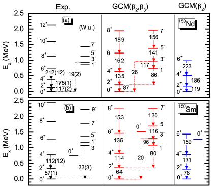
Figure 2: (Color online) Low-energy spectra of ¹⁵⁰Nd and ¹⁵⁰Sm. The numbers on arrows are $E2$ (solid line) and $E3$ (dashed line) transition strengths, in Weisskopf units. Data are from Ref. NND .

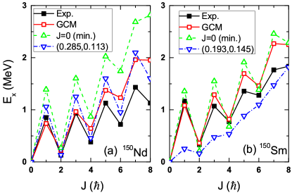
Figure 3: (Color online) Excitation energies of parity doublet states in ¹⁵⁰Nd (a) and ¹⁵⁰Sm (b). The available data ($\blacksquare$) are compared with the GCM results (${\color[rgb]{1,0,0}\square}$) and the results produced by the single-configuration of $J=0$ energy minimum (${\color[rgb]{0,1,0}\vartriangle}$) and by the configuration with deformation parameters determined by measured transition strengths $B(E2:0^{+}_{1}\to 2^{+}_{1})$ and $B(E3:0^{+}_{1}\to 3^{-}_{1})$ (${\color[rgb]{0,0,1}\triangledown}$) NND .

Figure 2 shows the low-lying energy spectra in ¹⁵⁰Nd and ¹⁵⁰Sm. The octupole degree of freedom reduces the $E2$ transition strengths between positive-parity states significantly in both nuclei. It worsens the agreement in ¹⁵⁰Nd but improves it in ¹⁵⁰Sm. Our GCM describes the negative-parity band built on the $1^{-}$ state rather well, despite overestimating the transition strength $B(E3:0^{+}_{1}\to 3^{-}_{1})$ in ¹⁵⁰Nd and underestimating it in ¹⁵⁰Sm.

Figure 3 compares the GCM excitation energies with those calculations that use a single symmetry-projected BCS state, either the one that corresponds to the $J=0$ energy minimum or the one with deformation parameters determined by the experimental $B(E2:0^{+}_{1}\to 2^{+}_{1})$ and $B(E3:0^{+}_{1}\to 3^{-}_{1})$ values NND . The GCM results that include the configuration-mixing effect are in much better agreement with the data than those based on a single BCS state. As spin increases, however, the GCM increasingly over-predicts the data, indicating that some important correlations are missing. Time-reversal-symmetry-breaking reference states, produced in a cranking calculation, would likely lower the energies of high-spin states Borrajo et al. (2015).

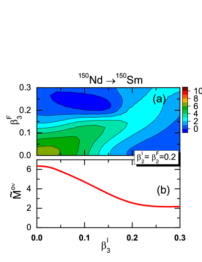
Figure 4: (Color online) Normalized nuclear matrix elements $\tilde{M}^{0\nu}$($q_{I},q_{F}$) for the neutrinoless double-beta decay of ¹⁵⁰Nd, where $\{q\}\equiv\{\beta_{2},\beta_{3}\}$. Panel (a) plots $\tilde{M}^{0\nu}$ versus the initial and final octupole deformation parameters, with the quadruple deformation parameters $\beta^{I}_{2}$ and $\beta^{F}_{2}$ fixed at 0.2 Panel (b) plots the same quantity with the restriction $\beta^{I}_{3}=\beta^{F}_{3}$.

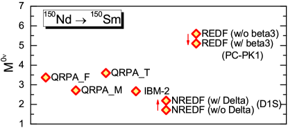
Figure 5: (Color online) The final matrix element $M^{0\nu}$ from the GCM calculation with and without Song et al. (2014) octupole shape fluctuations (REDF) and those of the QRPA (“QRPA_F” Fang et al. (2015), “QRPA_M” Mustonen and Engel (2013), “QRPA_T” Terasaki (2015)), the IMB-2 Barea and Iachello (2009), and the non-relativistic GCM, based on the Gogny D1S interaction, with Vaquero et al. (2013) and without Rodríguez and Martinez-Pinedo (2010) pairing fluctuations.

Figure 4 displays the normalized $0\nu\beta\beta$ matrix element between reference states, which we denote by $\tilde{M}^{0\nu}(q_{I},q_{F})$:

$$\tilde{M}^{0\nu}(q_{I},q_{F})$$ (15)

$$\equiv \dfrac{\langle q_{F}|\hat{\mathcal{O}}^{0\nu}\hat{P}^{J=0}\hat{P}^{N_{I}}\hat{P}^{Z_{I}}P^{\pi=+}|q_{I}\rangle}{\sqrt{\mathscr{N}^{0+}_{q_{I},q_{I}}\mathscr{N}^{0+}_{q_{F},q_{F}}}}\,,$$

with the norms $\mathscr{N}$ for each nucleus defined in Eq. (9). The function $\tilde{M}^{0\nu}(q_{I},q_{F})$ represents the contribution of particular initial and final configurations to the full matrix element. Panel (a) of Fig. 4 plots the function in the $\beta^{I}_{3},\beta^{F}_{3}$ plane, with $\beta^{I}_{2}$ and $\beta^{F}_{2}$ fixed at 0.2, the value that minimizes the energy in both nuclei. The figure shows that unequal octupole deformation in the two nuclei causes a rapid drop in the $0\nu\beta\beta$ matrix element. Panel (b) of Fig. 4 extracts the behavior of $\tilde{M}^{0\nu}$ from the diagonal of panel (a), where the octupole deformation is the same size in both nuclei. Increasing deformation causes even this diagonal contribution to drop, from 6.4 to 2.2 as $\beta_{3}$ increases to 0.3 At the configurations that minimize the projected energies, with both values of $\beta_{2}$ about 0.2 and both values of $\beta_{3}$ about 0.1, $\tilde{M}^{0\nu}$ is 4.76. At the configuration that best fits the experimental $B(E2:0^{+}_{1}\to 2^{+}_{1})$ and $B(E3:0^{+}_{1}\to 3^{-}_{1})$ values, corresponding to deformation parameters $\beta_{2}^{I}=0.285,\beta_{3}^{I}=0.113,\beta^{F}_{2}=0.193,\beta_{3}^{F}=0.145$, $\tilde{M}^{0\nu}$ is only 1.38.

As already discussed in Refs. Song et al. (2014); Yao et al. (2015b), $\tilde{M}^{0\nu}$ near spherical shapes is much larger than predicted by the Gogny D1S interaction Rodríguez and Martinez-Pinedo (2010). The difference arises at least in part from a difference in average pairing gaps, which for the neutrons in ¹⁵⁰Nd and ¹⁵⁰Sm are about 30% larger here than in Ref. Rodríguez and Martinez-Pinedo (2010) (even though the gaps are similar at the mean-field minima).

When all configurations are appropriately combined, we obtain a final value for the matrix element $M^{0\nu}(0^{+}_{1}\to 0^{+}_{1})$ of 5.2, which is just $7\%$ smaller than the result 5.6 obtained without octupole deformation Song et al. (2014). (The contributions from the $VV,AA,AP,PP$, and $MM$ terms are 1.03, 4.87, $-1.65$, 0.70, and 0.21, respectively). The small reduction, significantly less than what would result from the use of the single configuration in each nucleus that minimizes the energy (4.76) shows that shape fluctuations wash out the effects of octupole deformation. For the $0\nu\beta\beta$ decay to the excited $0^{+}$ state in ¹⁵⁰Sm, we find $M^{0\nu}(0^{+}_{1}\to 0^{+}_{2})=0.72$.

Figure 5 compares the ground-state to ground-state matrix elements $M^{0\nu}(0^{+}_{1}\to 0^{+}_{1})$ from several models. Our relativistic EDF-based GCM result is still about twice those of the deformed quasiparticle random phase approximation (QRPA) and the interacting boson model (IBM), and about three times that of the non-relativistic Gogny-based GCM. A more careful study of shell structure and pairing will help resolve the last discrepancy. And we can expect both GCM matrix elements to shrink once the isoscalar pairing amplitude is included as a generator coordinate Hinohara and Engel (2014); Menéndez et al. (2016).

IV Summary

We have used covariant multi-reference density functional theory to treat low-lying positive- and negative-parity states in ¹⁵⁰Nd and ¹⁵⁰Sm. The GCM mixes symmetry-projected states with different amounts of quadrupole and octupole deformation. The results indicate that octupole shape correlation have important dynamical effects, including the reduction of quadrupole collectivity in the low-lying states of both nuclei. As for $0\nu\beta\beta$ decay, static deformation, whether quadrupole or octupole, quenches the nuclear matrix element for that process, but shape fluctuations moderate the effect, so that the inclusion of octupole degrees of freedom ends up reducing the matrix element between the two nuclei considered here by only $7\%$.

References

- Argyriades et al. (2009) J. Argyriades, R. Arnold, C. Augier, J. Baker, A. S. Barabash, A. Basharina-Freshville, M. Bongrand, G. Broudin, V. Brudanin, A. J. Caffrey, E. Chauveau, Z. Daraktchieva, D. Durand, V. Egorov, N. Fatemi-Ghomi, R. Flack, P. Hubert, J. Jerie, S. Jullian, M. Kauer, S. King, A. Klimenko, O. Kochetov, S. I. Konovalov, V. Kovalenko, D. Lalanne, T. Lamhamdi, K. Lang, Y. Lemière, C. Longuemare, G. Lutter, C. Marquet, J. Martin-Albo, F. Mauger, A. Nachab, I. Nasteva, I. Nemchenok, F. Nova, P. Novella, H. Ohsumi, R. B. Pahlka, F. Perrot, F. Piquemal, J. L. Reyss, J. S. Ricol, R. Saakyan, X. Sarazin, L. Simard, F. Šimkovic, Y. Shitov, A. Smolnikov, S. Snow, S. Söldner-Rembold, I. Štekl, J. Suhonen, C. S. Sutton, G. Szklarz, J. Thomas, V. Timkin, V. Tretyak, V. Umatov, L. Vála, I. Vanyushin, V. Vasiliev, V. Vorobel, and T. Vylov (NEMO Collaboration), Phys. Rev. C 80, 032501 (2009).
- Bongrand (2015) M. Bongrand, Physics Procedia 61, 211 (2015), 13th International Conference on Topics in Astroparticle and Underground Physics, {TAUP} 2013.
- Casten and Zamfir (2001) R. F. Casten and N. V. Zamfir, Phys. Rev. Lett. 87, 052503 (2001).
- Krücken et al. (2002) R. Krücken, B. Albanna, C. Bialik, R. F. Casten, J. R. Cooper, A. Dewald, N. V. Zamfir, C. J. Barton, C. W. Beausang, M. A. Caprio, A. A. Hecht, T. Klug, J. R. Novak, N. Pietralla, and P. von Brentano, Phys. Rev. Lett. 88, 232501 (2002).
- Meng et al. (2005) J. Meng, W. Zhang, S. G. Zhou, H. Toki, and L. S. Geng, Euro. Phys. J. A 25, 23 (2005).
- Sheng and Guo (2005) Z. Q. Sheng and J.-Y. Guo, Mod. Phys. Lett. A 20, 2711 (2005).
- Nikšić et al. (2007) T. Nikšić, D. Vretenar, G. A. Lalazissis, and P. Ring, Phys. Rev. Lett. 99, 092502 (2007).
- Rodríguez-Guzmán and Sarriguren (2007) R. Rodríguez-Guzmán and P. Sarriguren, Phys. Rev. C 76, 064303 (2007).
- Rodriguez and Egido (2008) T. R. Rodriguez and J. L. Egido, Phys. Lett. B 663, 49 (2008).
- Robledo et al. (2008) L. M. Robledo, R. R. Rodríguez-Guzmán, and P. Sarriguren, Phys. Rev. C 78, 034314 (2008).
- Li et al. (2009) Z. P. Li, T. Nikšić, D. Vretenar, J. Meng, G. A. Lalazissis, and P. Ring, Phys. Rev. C 79, 054301 (2009).
- Urban et al. (1987) W. Urban, R. Lieder, W. Gast, G. Hebbinghaus, A. Kr?mer-Flecken, K. Blume, and H. H bel, Phys. Lett. B 185, 331 (1987).
- Friedrichs et al. (1992) H. Friedrichs, B. Schlitt, J. Margraf, S. Lindenstruth, C. Wesselborg, R. D. Heil, H. H. Pitz, U. Kneissl, P. von Brentano, R. D. Herzberg, A. Zilges, D. Häger, G. Müller, and M. Schumacher, Phys. Rev. C 45, R892 (1992).
- Bvumbi et al. (2013) S. P. Bvumbi, J. F. Sharpey-Schafer, P. M. Jones, S. M. Mullins, B. M. Nyakó, K. Juhász, R. A. Bark, L. Bianco, D. M. Cullen, D. Curien, P. E. Garrett, P. T. Greenlees, J. Hirvonen, U. Jakobsson, J. Kau, F. Komati, R. Julin, S. Juutinen, S. Ketelhut, A. Korichi, E. A. Lawrie, J. J. Lawrie, M. Leino, T. E. Madiba, S. N. T. Majola, P. Maine, A. Minkova, N. J. Ncapayi, P. Nieminen, P. Peura, P. Rahkila, L. L. Riedinger, P. Ruotsalainen, J. Saren, C. Scholey, J. Sorri, S. Stolze, J. Timar, J. Uusitalo, and P. A. Vymers, Phys. Rev. C 87, 044333 (2013).
- Nazarewicz and Tabor (1992) W. Nazarewicz and S. L. Tabor, Phys. Rev. C 45, 2226 (1992).
- Garrote et al. (1998) E. Garrote, J. L. Egido, and L. M. Robledo, Phys. Rev. Lett. 80, 4398 (1998).
- Babilon et al. (2005) M. Babilon, N. V. Zamfir, D. Kusnezov, E. A. McCutchan, and A. Zilges, Phys. Rev. C 72, 064302 (2005).
- Minkov et al. (2006) N. Minkov, P. Yotov, S. Drenska, W. Scheid, D. Bonatsos, D. Lenis, and D. Petrellis, Phys. Rev. C 73, 044315 (2006).
- Zhang et al. (2010) W. Zhang, Z. P. Li, S. Q. Zhang, and J. Meng, Phys. Rev. C 81, 034302 (2010).
- Robledo and Bertsch (2011) L. M. Robledo and G. F. Bertsch, Phys. Rev. C 84, 054302 (2011).
- Rodríguez-Guzmán et al. (2012) R. Rodríguez-Guzmán, L. M. Robledo, and P. Sarriguren, Phys. Rev. C 86, 034336 (2012).
- Nomura et al. (2014) K. Nomura, D. Vretenar, T. Nikšić, and B.-N. Lu, Phys. Rev. C 89, 024312 (2014).
- Nomura et al. (2015) K. Nomura, R. Rodríguez-Guzmán, and L. M. Robledo, Phys. Rev. C 92, 014312 (2015).
- Reinhard (1989) P. G. Reinhard, Rep. Prog. Phys. 52, 439 (1989).
- Ring (1996) P. Ring, Prog. Part. Nucl. Phys. 37, 193 (1996).
- Vretenar et al. (2005) D. Vretenar, A. Afanasjev, G. Lalazissis, and P. Ring, Phys. Rep. 409, 101 (2005).
- Meng et al. (2006) J. Meng, H. Toki, S. Zhou, S. Zhang, W. Long, and L. Geng, Prog. Part. Nucl. Phys. 57, 470 (2006).
- Geng et al. (2007) L. S. Geng, J. Meng, and H. Toki, Chin. Phys. Lett. 24, 1865 (2007).
- Guo et al. (2010) J.-Y. Guo, P. Jiao, and X.-Z. Fang, Phys. Rev. C 82, 047301 (2010).
- Lu et al. (2012) B.-N. Lu, E.-G. Zhao, and S.-G. Zhou, Phys. Rev. C 85, 011301 (2012).
- Li et al. (2013) Z. P. Li, B. Y. Song, J. M. Yao, D. Vretenar, and J. Meng, Phys. Lett. B 726, 866 (2013).
- Nikšić et al. (2006) T. Nikšić, D. Vretenar, and P. Ring, Phys. Rev. C 74, 064309 (2006).
- Yao et al. (2013) J. M. Yao, H. Mei, and Z. Li, Phys. Lett. B 723, 459 (2013).
- Wu et al. (2014) X. Y. Wu, J. M. Yao, and Z. P. Li, Phys. Rev. C 89, 017304 (2014).
- Wu and Zhou (2015) X. Y. Wu and X. R. Zhou, Phys. Rev. C 92, 054321 (2015).
- Yao et al. (2010) J. M. Yao, J. Meng, P. Ring, and D. Vretenar, Phys. Rev. C 81, 044311 (2010).
- Yao et al. (2011) J. M. Yao, H. Mei, H. Chen, J. Meng, P. Ring, and D. Vretenar, Phys. Rev. C 83, 014308 (2011).
- Yao et al. (2014) J. M. Yao, K. Hagino, Z. P. Li, J. Meng, and P. Ring, Phys. Rev. C 89, 054306 (2014).
- Yao et al. (2015a) J. M. Yao, E. F. Zhou, and Z. P. Li, Phys. Rev. C 92, 041304 (2015a).
- Zhou et al. (2016) E. F. Zhou, J. M. Yao, Z. P. Li, J. Meng, and P. Ring, Phys. Lett. B 753, 227 (2016).
- Hirsch et al. (1995) J. G. Hirsch, O. Castanos, and P. O. Hess, Nucl. Phys. A 582, 124 (1995).
- Chaturvedi et al. (2008) K. Chaturvedi, R. Chandra, P. K. Rath, P. K. Raina, and J. G. Hirsch, Phys. Rev. C 78, 054302 (2008).
- Fang et al. (2010) D.-L. Fang, A. Faessler, V. Rodin, and F. Šimkovic, Phys. Rev. C 82, 051301 (2010).
- Rodríguez and Martinez-Pinedo (2010) T. R. Rodríguez and G. Martinez-Pinedo, Phys. Rev. Lett. 105, 252503 (2010).
- Mustonen and Engel (2013) M. T. Mustonen and J. Engel, Phys. Rev. C 87, 064302 (2013).
- Song et al. (2014) L. S. Song, J. M. Yao, P. Ring, and J. Meng, Phys. Rev. C 90, 054309 (2014).
- Terasaki (2015) J. Terasaki, Phys. Rev. C 91, 034318 (2015).
- Yao et al. (2015b) J. M. Yao, L. S. Song, K. Hagino, P. Ring, and J. Meng, Phys. Rev. C 91, 024316 (2015b).
- Nikolaus et al. (1992) B. A. Nikolaus, T. Hoch, and D. G. Madland, Phys. Rev. C 46, 1757 (1992).
- Bürvenich et al. (2002) T. Bürvenich, D. G. Madland, J. A. Maruhn, and P.-G. Reinhard, Phys. Rev. C 65, 044308 (2002).
- Zhao et al. (2010) P. W. Zhao, Z. P. Li, J. M. Yao, and J. Meng, Phys. Rev. C 82, 054319 (2010).
- Gambhir et al. (1990) Y. K. Gambhir, P. Ring, and A. Thimet, Annals of Physics 198, 132 (1990).
- Krieger et al. (1990) S. J. Krieger, P. Bonche, H. Flocard, P. Quentin, and M. Weiss, Nucl. Phys. A 517, 275 (1990).
- Li et al. (2011) Z. Li, J. Xiang, J. M. Yao, H. Chen, and J. Meng, Int. J. Mod. Phys. E 20, 494 (2011).
- Tian et al. (2009) Y. Tian, Z. Ma, and P. Ring, Phys. Lett. B 676, 44 (2009).
- Ring and Schuck (1980) P. Ring and P. Schuck, The Nuclear Many-Body Problem (Springer-Verlag, 1980).
- Hill and Wheeler (1953) D. L. Hill and J. A. Wheeler, Phys. Rev. 89, 1102 (1953).
- Griffin and Wheeler (1957) J. J. Griffin and J. A. Wheeler, Phys. Rev. 108, 311 (1957).
- Rodriguez-Guzman et al. (2002) R. Rodriguez-Guzman, J. Egido, and L. Robledo, Nucl. Phys. A 709, 201 (2002).
- Lacroix et al. (2009) D. Lacroix, T. Duguet, and M. Bender, Phys. Rev. C 79, 044318 (2009).
- Duguet et al. (2009) T. Duguet, M. Bender, K. Bennaceur, D. Lacroix, and T. Lesinski, Phys. Rev. C 79, 044320 (2009).
- Fomenko (1970) V. N. Fomenko, J. Phys. A: Gen. Phys. 3, 8 (1970).
- Bender and Heenen (2008) M. Bender and P.-H. Heenen, Phys. Rev. C 78, 024309 (2008).
- Rodríguez and Egido (2010) T. R. Rodríguez and J. L. Egido, Phys. Rev. C 81, 064323 (2010).
- Avignone et al. (2008) F. T. Avignone, S. R. Elliott, and J. Engel, Rev. Mod. Phys. 80, 481 (2008).
- Haxton and Stephenson (1984) W. C. Haxton and G. J. Stephenson, Prog. Part. Nucl. Phys. 12, 409 (1984).
- Šimkovic et al. (1999) F. Šimkovic, G. Pantis, J. D. Vergados, and A. Faessler, Phys. Rev. C 60, 055502 (1999).
- (68) National Nuclear Data Center (NNDC) , http://www.nndc.bnl.gov/.
- Borrajo et al. (2015) M. Borrajo, T. R. Rodriguez, and J. L. Egido, Phys. Lett. B 746, 341 (2015).
- Fang et al. (2015) D.-L. Fang, A. Faessler, and F. Simkovic, Phys. Rev. C 92, 044301 (2015).
- Barea and Iachello (2009) J. Barea and F. Iachello, Phys. Rev. C 79, 044301 (2009).
- Vaquero et al. (2013) N. L. Vaquero, T. R. Rodríguez, and J. L. Egido, Phys. Rev. Lett. 111, 142501 (2013).
- Hinohara and Engel (2014) N. Hinohara and J. Engel, Phys. Rev. C 90, 031301 (2014).
- Menéndez et al. (2016) J. Menéndez, N. Hinohara, J. Engel, G. Martínez-Pinedo, and T. R. Rodríguez, Phys. Rev. C 93, 014305 (2016).