Isotoxal star-shaped polygonal voids and rigid inclusions in nonuniform antiplane shear fields.
Part I: Formulation and full-field solution

Abstract

An infinite class of nonuniform antiplane shear fields is considered for a linear elastic isotropic space and (non-intersecting) isotoxal star-shaped polygonal voids and rigid inclusions perturbing these fields are solved. Through the use of the complex potential technique together with the generalized binomial and the multinomial theorems, full-field closed-form solutions are obtained in the conformal plane. The particular (and important) cases of star-shaped cracks and rigid-line inclusions (stiffeners) are also derived. Except for special cases (addressed in Part II), the obtained solutions show singularities at the inclusion corners and at the crack and stiffener ends, where the stress blows-up to infinity, and is therefore detrimental to strength. It is for this reason that the closed-form determination of the stress field near a sharp inclusion or void is crucial for the design of ultra-resistant composites.

Keywords: v-notch, star-shaped crack, stress singularity, stress annihilation, invisibility, conformal mapping, complex variable method.

1 Introduction

The investigation of the perturbation induced by an inclusion (a void, or a crack, or a stiff insert) in an ambient stress field loading a linear elastic infinite space is a fundamental problem in solid mechanics, whose importance need not be emphasized. Usually this problem is analyzed with respect to uniform ambient stress fields [1, 5, 8, 13, 23, 25], although inhomogeneous, self-equilibrated stresses have also been considered [4, 6, 12, 32, 34, 39, 40]. The interplay between stress inhomogeneities and singularities generated at inclusion corners is important in the design of ultra-resistant composites, as stress singularities are known to be detrimental to strength. In fact, an extreme stress concentration, leading to material failure, has been shown by experiments to represent the counterpart of the mathematical concept of singularity [19, 20]. The determination of the conditions leading to stress relief around inclusions may introduce new perspectives in the development of composite materials.

The present article addresses the analytical, closed-form solution of isotoxal star-shaped polygonal voids and rigid inclusions in an elastic isotropic matrix loaded by inhomogeneous (but self-equilibrated) antiplane shear fields (which are introduced as polynomial in an explicit mechanical setting). The solution is obtained using the complex potential technique, with conformal mapping [23, 24, 25], which leads to a full-field determination of the stress field. The particular cases of infinitely thin star corners are also addressed, corresponding to star-shaped cracks and stiffeners (the latter also referred to as rigid-line inclusions). These patterns of multiple cracks are quite common, as three and four point star-shaped cracks are induced by triangular and Vickers pyramidal indenters [7, 9, 10] and can emerge during drying of colloidal suspensions in capillary tubes [14, 18]. Multiple radial crack patterns are generated after low speed impacts on brittle plates [38]. In Section 3, using the multinomial (and the generalized binomial) theorem, the full-field closed-form solutions for isotoxal star-shaped polygonal voids and rigid inclusions (and for star-shaped cracks and stiffeners) perturbing an inhomogeneous antiplane shear field are obtained, after the problem is posed and solved in its asymptotic form in Section 2. These results open the way to issues related to inclusion neutrality and in particular allows the discovery of ‘quasi-static invisibility’ and ‘stress annihilations’, whose treatment is deferred to Part II of this study [2], together with considerations of irregularities in the shape of the inclusions and the finiteness of the domain containing the inclusion.

The presented results, obtained in out-of-plane elasticity, provide also a solution for problems in thermal conductivity and electrostatics, due to the common governing equations expressed by the Laplacian.

2 Governing equations, polynomial far-field stress, and asymptotics

When anti-plane strain conditions prevail in a linear elastic solid, the gradient of the only non-vanishing displacement component, orthogonal to the $x_{1}$–$x_{2}$ plane and denoted by $w(x_{1},x_{2})$, defines the shear stress components (through the shear modulus $\mu$) as

$$\tau_{13}(x_{1},x_{2})=\mu\frac{\partial w(x_{1},x_{2})}{\partial x_{1}},\qquad\tau_{23}(x_{1},x_{2})=\mu\frac{\partial w(x_{1},x_{2})}{\partial x_{2}},$$ (1)

which are requested to satisfy the equilibrium equation in the absence of body forces,

$$\frac{\partial\tau_{13}(x_{1},x_{2})}{\partial x_{1}}+\frac{\partial\tau_{23}(x_{1},x_{2})}{\partial x_{2}}=0.$$ (2)

In addition to the equilibrium equations, compatibility (or, in other words, the Schwarz theorem for function $w$) requires

$$\frac{\partial\tau_{13}(x_{1},x_{2})}{\partial x_{2}}-\frac{\partial\tau_{23}(x_{1},x_{2})}{\partial x_{1}}=0.$$ (3)

Note that for the antiplane problem, one eigenvalue of the stress tensor is null and the other two have opposite signs. The absolute value of the two non-null eigenvalues is

$$\tau=\sqrt{\left(\tau_{13}\right)^{2}+\left(\tau_{23}\right)^{2}}.$$ (4)

2.1 An infinite class of antiplane shear fields

A class of remote anti-plane loadings is considered for an infinite elastic solid containing an inclusion, as defined by the following polynomial stress field of $m$-th order ($m\in\mathbb{N}$)

$$\tau_{13}^{\infty(m)}(x_{1},x_{2})={\sum_{j=0}^{m}}b_{j}^{(m)}x_{1}^{m-j}x_{2}^{j},\qquad\tau_{23}^{\infty(m)}(x_{1},x_{2})={\sum_{j=0}^{m}}c_{j}^{(m)}x_{1}^{m-j}x_{2}^{j},$$ (5)

where $b^{(m)}_{j}$ and $c^{(m)}_{j}$ are constants ($j=0,...,m$). Because the polynomial stress field (5) has to satisfy both the equilibrium equation (2) and the compatibility equation (3), all the constants $b^{(m)}_{j}$ and $c^{(m)}_{j}$ are linearly dependent on $b^{(m)}_{0}$ and $c^{(m)}_{0}$ as follows

$$\begin{array}[]{llll}&b_{j}^{(m)}=(-1)^{\frac{j}{2}}\dfrac{m!}{j!(m-j)!}b_{0}^{(m)},&c_{j}^{(m)}=(-1)^{\frac{j}{2}}\dfrac{m!}{j!(m-j)!}c_{0}^{(m)}\,,&\forall\,\,\mbox{even}\,\,j\in[0;m],\\[14.22636pt] &b_{j}^{(m)}=(-1)^{\frac{j-1}{2}}\dfrac{m!}{j!(m-j)!}c_{0}^{(m)},&c_{j}^{(m)}=(-1)^{\frac{j+1}{2}}\dfrac{m!}{j!(m-j)!}b_{0}^{(m)}\,,&\forall\,\,\mbox{odd}\,\,j\in[0;m].\end{array}$$ (6)

Note that the constants $b^{(m)}_{0}$ and $c^{(m)}_{0}$ represent a measure of the remote (or, in the inclusion problem, the ‘unperturbed’) stress state along the $x_{1}$ axis,

$$\tau_{13}^{\infty(m)}(x_{1},0)=b_{0}^{(m)}x_{1}^{m},\qquad\tau_{23}^{\infty(m)}(x_{1},0)=c_{0}^{(m)}x_{1}^{m},$$ (7)

so that $b_{0}^{(0)}$ and $c_{0}^{(0)}$ are the loading constants defining the usual uniform Mode III, Fig. 1 (upper part),

$$\tau_{13}^{\infty(0)}(x_{1},0)=b_{0}^{(0)},\qquad\tau_{23}^{\infty(0)}(x_{1},0)=c_{0}^{(0)}.$$ (8)

With the only exception of the case $m=0$, the two remote shear stress components are affected by both constants $b_{0}^{(m)}$ and $c_{0}^{(m)}$. For example, in the case of linear remote loading ($m$=1), Fig. 1 (lower part), the remote field is defined by

$$\tau_{13}^{\infty(1)}(x_{1},x_{2})=b_{0}^{(1)}x_{1}+c_{0}^{(1)}x_{2},\qquad\tau_{23}^{\infty(1)}(x_{1},x_{2})=c_{0}^{(1)}x_{1}-b_{0}^{(1)}x_{2}.$$ (9)

Note that the introduced polynomial fields can be used to reconstruct through series a general self-equilibrated remote loading. Therefore, due to the superposition principle, the solution obtained in the next sections also describes the mechanical fields under general Mode III remote loadings.

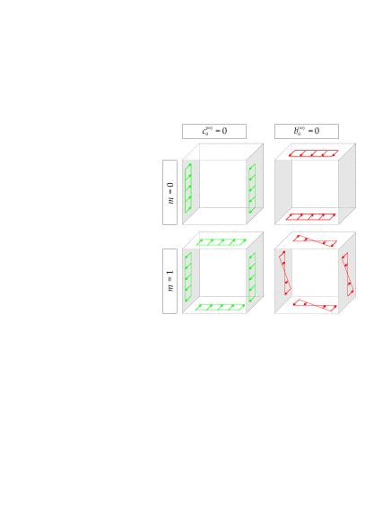
Figure 1: The cases of uniform ($m=0$, upper part) and linear ($m=1$, lower part) remote (self-equilibrated) loading conditions described by the constant $b_{0}^{(m)}$ (left) and $c_{0}^{(m)}$ (right), eqn (5).

It is instrumental to express the polynomial stress field (5) in two further reference systems, one Cartesian and the other polar. In particular, with reference to a $\hat{x}_{1}$–$\hat{x}_{2}$ Cartesian coordinate system obtained through a rotation of an angle $\gamma$ of a $x_{1}$–$x_{2}$ system, the polynomial stress field can be expressed as

$$\hat{\tau}_{13}^{\infty(m)}(\hat{x}_{1},\hat{x}_{2})={\sum_{j=0}^{m}}\hat{b}_{j}^{(m)}\hat{x}_{1}^{m-j}\hat{x}_{2}^{j},\qquad\hat{\tau}_{23}^{\infty(m)}(\hat{x}_{1},\hat{x}_{2})={\sum_{j=0}^{m}}\hat{c}_{j}^{(m)}\hat{x}_{1}^{m-j}\hat{x}_{2}^{j},$$ (10)

where the loading constants $\hat{b}^{(m)}_{0}$ and $\hat{c}^{(m)}_{0}$ are linearly dependent on the constants $b^{(m)}_{0}$ and $c^{(m)}_{0}$ as follows

$$\begin{array}[]{ll}\hat{b}^{(m)}_{0}=b_{0}^{(m)}\cos((m+1)\gamma)+c_{0}^{(m)}\sin((m+1)\gamma),\\[11.38109pt] \hat{c}^{(m)}_{0}=c_{0}^{(m)}\cos((m+1)\gamma)-b_{0}^{(m)}\sin((m+1)\gamma).\end{array}$$ (11)

With reference to a polar coordinate system $(r,\theta)$ centered at the origin of the $x_{1}$–$x_{2}$ axes, the polynomial stress field (5) can be rewritten as

$$\begin{cases}\begin{array}[]{cll}\tau_{r3}^{\infty(m)}(r,\theta)&=&r^{m}\left[b^{(m)}_{0}\cos\left((m+1)\theta\right)+c^{(m)}_{0}\sin\left((m+1)\theta\right)\right],\\[17.07164pt] \tau_{\theta 3}^{\infty(m)}(r,\theta)&=&r^{m}\left[c^{(m)}_{0}\cos\left((m+1)\theta\right)-b^{(m)}_{0}\sin\left((m+1)\theta\right)\right],\end{array}\end{cases}$$ (12)

corresponding to the displacement

$$w^{\infty(m)}(r,\theta)=\frac{r^{m+1}}{\mu(m+1)}\left[b^{(m)}_{0}\cos\left((m+1)\theta\right)+c^{(m)}_{0}\sin\left((m+1)\theta\right)\right].$$ (13)

Finally, it can be noted that the modulus of the principal stress (4) is independent of the circumferential angle $\theta$

$$\tau^{\infty(m)}(r)=r^{m}\sqrt{\left[b^{(m)}_{0}\right]^{2}+\left[c^{(m)}_{0}\right]^{2}},$$ (14)

so that the level sets of the modulus of the (unperturbed) shear stress are concentric circles centered at the origin of the axes.

2.2 Asymptotic expansion near the vertex of a void or a rigid inclusion

A vertex of a void or a rigid inclusion is considered (defined by the semi-angle $\alpha$ exterior to the inclusion, Fig. 2, right), with reference to a polar coordinate system $(\rho,\vartheta)$ centered at the inclusion corner, where $\vartheta\in(-\alpha,\alpha)$ measures the angle from the symmetry axis. Following [27]–[31], the solution of the general out-of-plane problem can be decomposed in its symmetric $w^{\textup{S}}(\rho,\vartheta)=w^{\textup{S}}(\rho,-\vartheta)$ and antisymmetric $w^{\textup{A}}(\rho,\vartheta)=-w^{\textup{A}}(\rho,-\vartheta)$ terms,

$$w(\rho,\vartheta)=w^{\textup{S}}(\rho,\vartheta)+w^{\textup{A}}(\rho,\vartheta),$$ (15)

which, considering equations (1)–(3), assume the following expressions in polar coordinates,

$$\begin{array}[]{lll}w^{\textup{S}}(\rho,\vartheta)=\displaystyle D^{\textup{S}}\rho^{1+\lambda^{\textup{S}}}\cos\left[\left(1+\lambda^{\textup{S}}\right)\vartheta\right],\\[11.38109pt] w^{\textup{A}}(\rho,\vartheta)=D^{\textup{A}}\displaystyle\rho^{1+\lambda^{\textup{A}}}\sin\left[\left(1+\lambda^{\textup{A}}\right)\vartheta\right],\end{array}$$ (16)

and, through the isotropic elastic constitutive relation (1), the following stress field representations are obtained as

$$\begin{array}[]{lll}\tau_{\rho 3}^{\textup{S}}(\rho,\vartheta)=\mu\displaystyle\,D^{\textup{S}}\,(1+\lambda^{\textup{S}})\rho^{\lambda^{\textup{S}}}\cos\left[(1+\lambda^{\textup{S}})\vartheta\right],\\[11.38109pt] \tau_{\vartheta 3}^{\textup{S}}(\rho,\vartheta)=-\mu\displaystyle\,D^{\textup{S}}\,(1+\lambda^{\textup{S}})\rho^{\lambda^{\textup{S}}}\sin\left[(1+\lambda^{\textup{S}})\vartheta\right],\\[11.38109pt] \tau_{\rho 3}^{\textup{A}}(\rho,\vartheta)=\mu\displaystyle\,D^{\textup{A}}\,(1+\lambda^{\textup{A}})\rho^{\lambda^{\textup{A}}}\sin\left[(1+\lambda^{\textup{A}})\vartheta\right],\\[11.38109pt] \tau_{\vartheta 3}^{\textup{A}}(\rho,\vartheta)=\mu\displaystyle\,D^{\textup{A}}\,(1+\lambda^{\textup{A}})\rho^{\lambda^{\textup{A}}}\cos\left[(1+\lambda^{\textup{A}})\vartheta\right],\end{array}$$ (17)

where $D^{\textup{S}}$ and $D^{\textup{A}}$ are constants (to be defined in relation to the remote loading), while $\lambda^{\textup{S}}$ and $\lambda^{\textup{A}}$ are the eigenvalues of the characteristic equations for the symmetric and antisymmetric problem, respectively, with $\{\lambda^{\textup{S}},\lambda^{\textup{A}}\}>-1$, to satisfy the requirement of finiteness of the local elastic strain energy. These eigenvalues can be defined through the boundary condition imposed at the inclusion boundary and are crucial to the asymptotic description of stress fields around the inclusion vertex.

The apexes ${}^{\text{\tiny\char 73}}$ and ${}^{\text{\tiny\char 72}}$ will be used to distinguish between values assigned to voids and to rigid inclusions, respectively. The null traction or null displacement boundary conditions at $\theta=\pm\alpha$, holding respectively for the former and the latter problem, can be expressed as [36]

$$\tau^{\text{\tiny\char 73}}_{\theta 3}(\rho,\pm\alpha)=0,\qquad w^{\text{\tiny\char 72}}(\rho,\pm\alpha)=0,$$ (18)

leading to the following characteristic equations

$$\begin{array}[]{lll}\sin\left[\alpha\left(1+\lambda^{\!\text{\tiny\char 73}\textup{S}}\right)\right]=0,\qquad\cos\left[\alpha\left(1+\lambda^{\!\text{\tiny\char 73}\textup{A}}\right)\right]=0,\\[17.07164pt] \cos\left[\alpha\left(1+\lambda^{\!\text{\tiny\char 72}\textup{S}}\right)\right]=0,\qquad\sin\left[\alpha\left(1+\lambda^{\!\text{\tiny\char 72}\textup{A}}\right)\right]=0,\end{array}\qquad j\in\mathbb{N},$$ (19)

and from which two countably infinite set of eigenvalues $\lambda^{\text{\tiny\char 73}\textup{A}}_{j}$, $\lambda^{\text{\tiny\char 72}\textup{A}}_{j}$, $\lambda^{\text{\tiny\char 73}\textup{S}}_{j}$ and $\lambda^{\text{\tiny\char 72}\textup{S}}_{j}$ are obtained as

$$\begin{cases}\lambda^{\!\text{\tiny\char 73}\textup{S}}_{j}(\alpha)=\lambda^{\!\text{\tiny\char 72}\textup{A}}_{j}(\alpha)=-1+\dfrac{j\pi}{\alpha},\\[17.07164pt] \lambda^{\!\text{\tiny\char 73}\textup{A}}_{j}(\alpha)=\lambda^{\!\text{\tiny\char 72}\textup{S}}_{j}(\alpha)=-1+\dfrac{(2j-1)\pi}{2\alpha},\end{cases}\qquad j\in\mathbb{N}.$$ (20)

The mechanical fields at small distances from the inclusion are ruled by the leading-order term in the symmetric and antisymmetric asymptotic expansions (16), which correspond to $j=1$

$$\begin{cases}\lambda^{\!\text{\tiny\char 73}\textup{S}}_{1}(\alpha)=\lambda^{\!\text{\tiny\char 72}\textup{A}}_{1}(\alpha)=-1+\dfrac{\pi}{\alpha}\geq 0,\\[14.22636pt] \lambda^{\!\text{\tiny\char 73}\textup{A}}_{1}(\alpha)=\lambda^{\!\text{\tiny\char 72}\textup{S}}_{1}(\alpha)=-1+\dfrac{\pi}{2\alpha}\geq\displaystyle-\frac{1}{2},\end{cases}$$ (21)

and are reported in Fig. 2 (left) as a function of exterior semi-angle $\alpha$. Note that the following property holds true

$$\lambda^{\!\text{\tiny\char 73}\textup{S}}_{1}(\alpha)=\lambda^{\!\text{\tiny\char 72}\textup{A}}_{1}(\alpha)\,\,>\,\,\lambda^{\!\text{\tiny\char 73}\textup{A}}_{1}(\alpha)=\lambda^{\!\text{\tiny\char 72}\textup{S}}_{1}(\alpha).$$ (22)

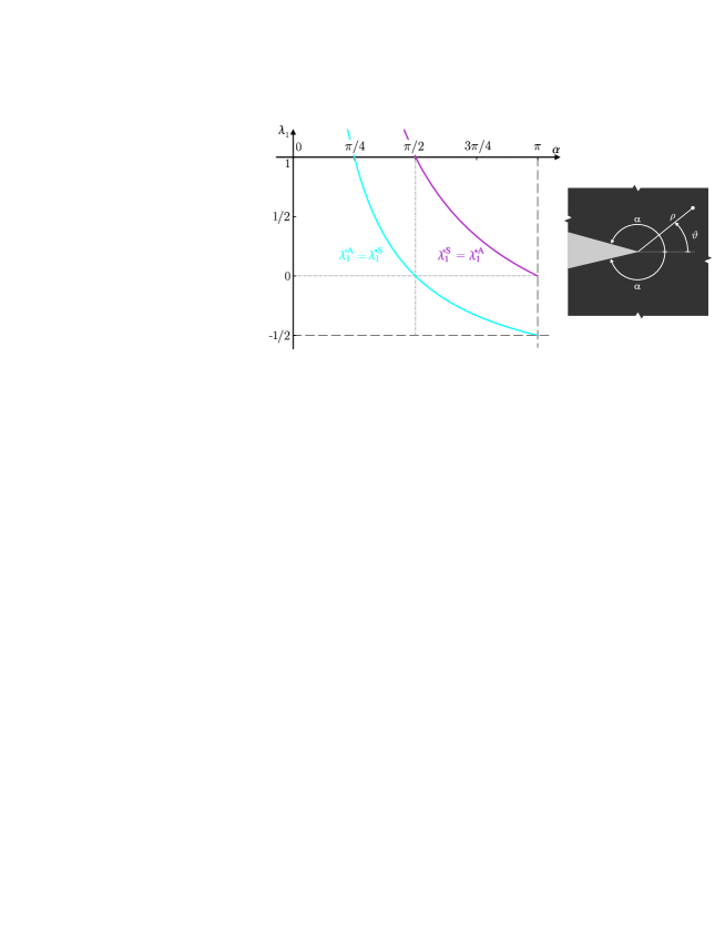
Figure 2: (left) First eigenvalue $\lambda_{1}$, guiding the leading-order term in the asymptotic description of symmetric and antisymmetric parts of mechanical fields (16) in the neighborhood of the inclusion vertex, as a function of the semi-angle $\alpha$ exterior to the inclusion (right).

The range of variation of the values $\lambda_{1}$ for different values of the exterior semi-angle $\alpha$ is summarized in Tab. 1 and reported in Fig. 2 (left), from which it can be noted that the stress field has:

• a singular leading-order term for antisymmetric notch/symmetric wedge problems when $\alpha\in\left(\pi/2,\pi\right]$ (in particular a square-root singularity is attained for $\alpha=\pi$, corresponding to antisymmetric crack/symmetric stiffener problems);

• a constant (zeroth-order) term for antisymmetric notch/symmetric wedge problems when $\alpha=\pi/2$ and for symmetric notch/antisymmetric wedge problems when $\alpha=\pi$. Such a constant is usually called T-stress in in-plane and S-stress in out-of-plane [15, 21, 22] crack problems;

• a non-singular leading-order term for symmetric notch/antisymmetric wedge problems when $\alpha<\pi$ and for antisymmetric notch/symmetric wedge problems when $\alpha<\pi/2$.

The above-listed observations are crucial for the understanding of the occurrence of stress singularity or of stress annihilation at the vertices of polygonal void and rigid inclusions, as shown in Part II.

$\alpha$	$\in\left(0,\dfrac{\pi}{2}\right)$	$\dfrac{\pi}{2}$	$\in\left(\dfrac{\pi}{2},\pi\right)$	$\pi$
$\lambda^{\!\text{\tiny\char 73}\textup{S}}_{1}(\alpha)=\lambda^{\!\text{\tiny\char 72}\textup{A}}_{1}(\alpha)$	$>1$	1	$\in(0,1)$	0
$\lambda^{\!\text{\tiny\char 73}\textup{A}}_{1}(\alpha)=\lambda^{\!\text{\tiny\char 72}\textup{S}}_{1}(\alpha)$	$>0$	0	$\in\left(-\dfrac{1}{2},0\right)$	$-\dfrac{1}{2}$

Table 1: Ranges of the first eigenvalue $\lambda_{1}$, defining the leading-order term in the description of symmetric and antisymmetric parts of the displacement field $w$, eqn (16)₁, for different ranges of exterior semi-angle $\alpha$ (Fig 2, right).

3 Full-field solution

The full-field solution for non-intersecting isotoxal star polygonal voids and rigid inclusions embedded in an isotropic elastic material subject to the generalized anti-plane remote polynomial stress field (5) is obtained through the complex potential technique generalizing the solution by Kohno and Ishikawa [17]. Considering the constitutive relation (1), equilibrium in the absence of body-forces (2) can be expressed in terms of the displacement field $w$ as the Laplace equation

$$\nabla^{2}w\left(x_{1},x_{2}\right)=0,$$ (23)

so that, introducing a complex potential $f(z)$, function of the complex variable $z=x_{1}+\mbox{${\mathrm{i}}$}x_{2}$ (where ${\mathrm{i}}$ is the imaginary unit), such that

$$w=\frac{1}{\mu}{\rm Re}[f(z)],$$ (24)

and, considering the Cauchy-Riemann conditions for analytic functions, the stress-potential relationship can be written as

$$\tau_{13}-\mbox{${\mathrm{i}}$}\tau_{23}=f^{\prime}(z),$$ (25)

so that the out-of-plane resultant shear force $F_{\stackrel{{\scriptstyle\frown}}{{BC}}}$ along an arc $\stackrel{{\scriptstyle\frown}}{{BC}}$ is

$$F_{\stackrel{{\scriptstyle\frown}}{{BC}}}={\int^{C}_{B}}\left(\tau_{13}\,\mathrm{d}x_{2}-\tau_{23}\,\mathrm{d}x_{1}\right)={\rm Im}\left[f(z_{C})-f(z_{B})\right].$$ (26)

The complex potential $f(z)$ can be considered as the sum of the unperturbed potential $f^{\infty}(z)$, which is the solution in the absence of the inclusion, and the perturbed one, $f^{p}(z)$, introduced to recover the boundary condition along the inclusion boundary,

$$f(z)=f^{\infty}(z)+f^{p}(z).$$ (27)

Using the polynomial description (5) for the self-equilibrated remote stress field $\tau_{13}^{\infty(m)}$ and $\tau_{23}^{\infty(m)}$, the unperturbed potential is given as

$$f^{\infty}(z,m)=T^{(m)}z^{m+1}\,,$$ (28)

where

$$T^{(m)}=\frac{b^{(m)}_{0}-\mbox{${\mathrm{i}}$}\,c^{(m)}_{0}}{m+1},$$ (29)

which in the particular case of uniform antiplane shear load, $m=0$, reduces to [17] (their equation (20)).

Considering now the presence of the inclusion, it is instrumental to define the conformal mapping $z=\omega(\zeta)$, which transforms the boundary of the inclusion in the physical plane into a circle of unit radius within the conformal plane. In the conformal plane, the complex potential

$$g(\zeta)=f(\omega(\zeta)),$$ (30)

is introduced, so that equations (24), (25) and (26) become

$$w=\frac{1}{\mu}{\rm Re}[g(\zeta)],\qquad\tau_{13}-\mbox{${\mathrm{i}}$}\tau_{23}=\frac{g^{\prime}(\zeta)}{\omega^{\prime}(\zeta)},\qquad F_{\stackrel{{\scriptstyle\frown}}{{BC}}}={\rm Im}\left[g(\zeta_{B})-g(\zeta_{C})\right].$$ (31)

The displacement and stress fields in the physical domain can be obtained once the inclusion shape is specified.

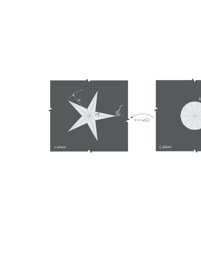
Figure 3: Infinite plane containing a $n$-pointed isotoxal star-shaped polygon inscribed in a circle of radius $a$. The polygon is defined by the semi-angle $\xi\pi$ at the isotoxal-points ($z$-plane) and is conformally mapped onto an infinite plane with a circular inclusion of unit radius ($\zeta$-plane) using the Schwarz-Christoffel formula (33). Note the local reference systems $z^{*}=z-a$ and $\zeta^{*}=\zeta-1$ defined in the two planes.

Rigid inclusions and voids are considered of isotoxal polygonal star shape, see Fig. 3 (left), embedded in infinite elastic matrix. An isotoxal polygonal star is defined by the number $N$ of vertices and a number $n=N/2$ of points. Note that $N\geq 4$ is always even, while $n\geq 2$ is an integer, so that a polygon (for instance a triangle, characterized by $N=6$ and $n=3$) is viewed as a degenerate star (for instance a three-pointed star, having $N=6$ and $n=3$). Introducing $\beta_{j}$ as the fraction of the angle $\pi$ measuring the $j$-th angle exterior to $j$-th vertex of the inclusion (for instance an equilateral triangle has $\beta_{1}=\beta_{3}=\beta_{5}=5/3$ and $\beta_{0}=\beta_{2}=\beta_{4}=1$), the following property holds true

$$\sum_{j=0}^{2n-1}\beta_{j}=2(n+1).$$ (32)

With reference now to a isotoxal polygonal star inclusion defined by $n$ points, the Schwarz-Christoffel conformal mapping (see [37] and [33]) is used to map the exterior region of the inclusion (within the physical $z-plane$) onto the exterior region of the unit circle (within the conformal $\zeta-plane$), namely

$$\begin{array}[]{cll}\omega(\zeta)&=&\displaystyle a\Omega\int^{\zeta}_{1}\left[\frac{1}{\sigma^{2}}\prod^{2n-1}_{j=0}\left(\sigma-k_{j}\right)^{\beta_{j}-1}\right]\,\mathrm{d}\sigma,\end{array}$$ (33)

where $a$ is the radius of the circle inscribing the inclusion, $\Omega$ is the scaling factor of the inclusion, $k_{j}$ is the pre-image of the $j$-th polygon vertex in the $\zeta$ plane.

The first derivative of the conformal mapping (33) becomes

$$\omega^{\prime}(\zeta)=\displaystyle a\Omega\frac{1}{\zeta^{2}}\prod^{2n-1}_{j=0}\left(\zeta-k_{j}\right)^{\beta_{j}-1}.$$ (34)

Further exploiting the identity (32), the first derivative of the conformal mapping (34) can be rewritten as

$$\omega^{\prime}(\zeta)=\displaystyle a\Omega\prod^{2n-1}_{j=0}\left(1-\frac{k_{j}}{\zeta}\right)^{\beta_{j}-1}.$$ (35)

With reference to a $n$-pointed isotoxal star polygon, see Fig. 3, the pre-images and the exterior angles $\beta_{j}$ appearing in equation (35) are respectively given by

$$k_{j}=e^{\mbox{${\mathrm{i}}$}\dfrac{j\pi}{n}}\qquad\mbox{and}\qquad\beta_{j}=\left\{\begin{array}[]{llll}2(1-\xi)&\mbox{if }\,\,j\,\,\,\mbox{is even}\\[11.38109pt] 2\left(\xi+1/n\right)&\mbox{if}\,\,j\,\,\,\mbox{is odd}\end{array}\right.\qquad j=0,...,2n-1,$$ (36)

where $\xi$ is the fraction of $\pi$ of the semi-angle at the isotoxal-points, restricted to the following set

$$\xi\in\left[0,\frac{1}{2}-\frac{1}{n}\right],$$ (37)

and that can be used to define the inclusion sharpness, starting from $\xi=0$, which corresponds to zero-thickness (infinite sharpness) inclusion, ending with $\xi=1/2-1/n$ corresponding to $n$-sided regular polygonal case.

From the definition (36)₁ of the pre-images $k_{j}$ (as the complex $n$-th roots of the positive and negative unity), the following identities, which will become useful later, can be derived

$$\prod_{j=0}^{n-1}\left(\zeta-k_{2j}\right)=\zeta^{n}-1,\qquad\prod_{j=1}^{n}\left(\zeta-k_{2j-1}\right)=\zeta^{n}+1,$$ (38)

which can be written in an equivalent and useful form, for the future calculations, as given below

$$\prod_{j=0}^{n-1}\left(1-\frac{k_{2j}}{\zeta}\right)=1-\frac{1}{\zeta^{n}},\qquad\prod_{j=1}^{n}\left(1-\frac{k_{2j-1}}{\zeta}\right)=1+\frac{1}{\zeta^{n}}.$$ (39)

The particular case of an $n$-pointed star polygon is identified through the Schläfli symbol $\left|n/\mathcal{S}\right|$ involving the density, or starriness, $\mathcal{S}\in\mathbb{N}_{1}$, which is subject to the constraint $\mathcal{S}<n/2$, see [16, 11]. Therefore, for star polygons, the following relation

$$\xi=\frac{1}{2}-\frac{\mathcal{S}}{n},$$ (40)

holds true, so that a regular $n$-sided polygon is recovered when $\mathcal{S}=1$, see equation (37). Now $\mathcal{S}$ controls the sharpness, so that the higher is $\mathcal{S}$, the sharper is the star, as shown in Fig. 4. In the limit case $\xi=0$ the star-shaped crack or stiffener is obtained (Fig. 5).

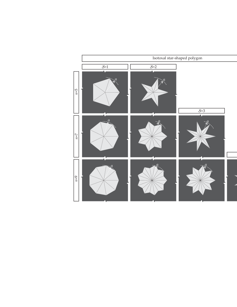
Figure 4: $n$-pointed isotoxal star-shaped polygons ($n=\{5,7,9\}$, from the upper part to the lower) inscribed in a circle of radius $a$ can be used to describe inclusions in the form of $n$-sided regular polygons and $n$-pointed regular stars with density $\mathcal{S}$ ($=\{1,2,3,4\}$, from left to right), within an infinite elastic plane. Note that, for a fixed $n$, the density parameter $\mathcal{S}$ can vary only within a finite range of natural numbers $\mathcal{S}<n/2$.

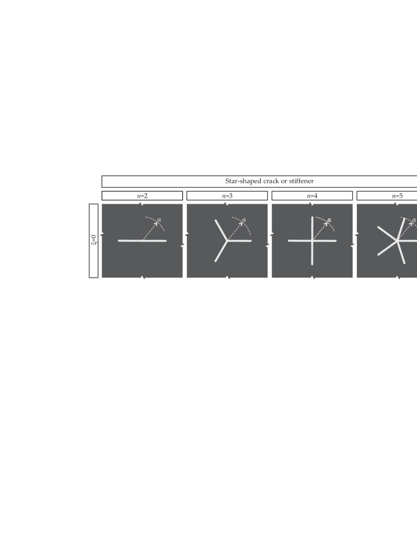
Figure 5: $n$-pointed star-shaped cracks/stiffeners, obtained in the limit of $\xi=0$ of isotoxal star-shaped polygons.

The generic conformal mapping (33) can be expressed through the following Laurent series ([25] and [24])

$$\omega(\zeta)=a\Omega\left(\zeta+\sum^{\infty}_{j=1}\frac{d_{j}}{\zeta^{j}}\right)\,,$$ (41)

where $d_{j}$ are complex constants depending on the inclusion shape.

In the following subsections, the conformal mappings for $n$-pointed star shaped cracks and stiffeners (zero-thickness, $\xi=0$) and isotoxal star polygonal voids or rigid inclusions (non-zero thickness, $\xi\neq 0$) will be obtained as special cases of the Laurent series as

$$\omega(\zeta,\xi,n)=a\Omega(n,\xi)\sum^{\infty}_{j=0}d_{1-jn}(\xi)\,\zeta^{1-jn}\,,$$ (42)

where the scaling factor $\Omega(n,\xi)$ and the constants $d_{1-jn}(\xi)$ will be given specific expressions. It is noteworthy that ‘$jn$’ denotes the multiplication $j\times n$ between the index $j$ and the number of points $n$.

3.1 Star-shaped crack and stiffener

An $n$-pointed star-shaped crack or a star-shaped stiffener can be obtained as the limit case of a isotoxal star polygon with an inifinte sharpness i.e. $\xi=0$, see Fig. 5.

Considering now a $n$-pointed regular star-shaped crack or rigid line inclusion and introducing $\xi=0$ in the definition (36)₂, the first derivative of the conformal mapping (35), together with equation (39), simplifies to

$$\omega^{\prime}(\zeta,n)=\displaystyle a\Omega(n)\,\left(1-\frac{1}{\zeta^{n}}\right)\left(1+\frac{1}{\zeta^{n}}\right)^{\frac{2-n}{n}},$$ (43)

where $\Omega(n)$ is a function of the number $n$ of star points given as

$$\Omega(n)=\displaystyle\frac{1}{\sqrt[n]{4}}\quad\in\,\,\left[\frac{1}{2}\,,1\right),$$ (44)

for which the lower bound is obtained for $n=2$ (line inclusions, crack or stiffener) while the upper bound corresponds to a circle, $n\rightarrow\infty$.

From the integration of equation (43), the mapping function can be obtained as

$$\omega(\zeta,n)=\displaystyle\frac{a}{\sqrt[n]{4}}\,\zeta\left(1+\frac{1}{\zeta^{n}}\right)^{\frac{2}{n}},$$ (45)

which, using the generalized binomial theorem, can be expressed as

$$\omega(\zeta,n)=\frac{a}{\sqrt[n]{4}}\sum^{\infty}_{j=0}\,\left[\prod_{k=0}^{j-1}\displaystyle\left(\frac{2}{n}-k\right)\right]\,\frac{\zeta^{1-jn}}{j!}\,,$$ (46)

namely, the Laurent series (42) with the complex coefficients $d_{1-jn}$ defined as

$$d_{1-jn}=\frac{1}{j!}\prod_{k=0}^{j-1}\displaystyle\left(\frac{2}{n}-k\right).$$ (47)

In the special case of a simple crack or a rigid line inclusion ($n=2$), equation (45), as well as the Laurent series (46), reduces to the well-known conformal mapping function

$$\omega(\zeta)=\displaystyle\frac{a}{2}\left(\zeta+\frac{1}{\zeta}\right).$$ (48)

To derive the complex potential (30) for star-shaped cracks and stiffeners, it is instrumental to introduce $t$ and $q$, functions of $m$ and $n$ as

$$t=\frac{2(m+1)}{n},\qquad q=\left\lfloor\frac{m+1}{n}\right\rfloor,$$ (49)

where the dependence on $m$ and $n$ is omitted for simplicity and the symbol $\lfloor\cdot\rfloor$ stands for the integer part of the relevant argument. By means of the generalized binomial theorem, the unperturbed potential can be expressed as

$$g^{\infty}(\zeta,n,m)=\frac{a^{m+1}\,\,T^{(m)}}{2^{t}}\sum_{j=0}^{\infty}\left(\prod_{l=0}^{j-1}t-l\right)\,\frac{\zeta^{m+1-jn}}{j!}.$$ (50)

By imposing the null traction resultant condition $F_{\stackrel{{\scriptstyle\frown}}{{BC}}}=0$ for a crack ($\chi=1$), or the rigid-body displacement condition $w_{B}=w_{C}$ for a rigid line inclusion ($\chi=-1$), for every pairs of points $B$ and $C$ along the boundary of the unit circle in the conformal plane, the perturbed complex potential $g^{p(m)}$ is obtained as

$$g^{p}(\zeta,n,m)=\frac{a^{m+1}}{2^{t}}\left\{\chi\overline{T^{(m)}}\left[-\frac{\delta_{m+1,qn}}{q!}\prod_{l=0}^{q-1}(t-l)\,\,+\sum_{j=0}^{q}\,\left(\prod_{l=0}^{j-1}t-l\right)\frac{1}{j!\,\zeta^{m+1-jn}}\right]-T^{(m)}\sum_{j=q+1}^{\infty}\,\left(\prod_{l=0}^{j-1}t-l\right)\frac{1}{j!\,\zeta^{jn-m-1}}\right\},$$ (51)

where $\delta_{m+1,qn}$ is Kronecker delta, so that ‘$qn$’ is a single index corresponding to the multiplication $q\times n$ between the two indices $q$ and $n$.

The complex potential follows from the sum of the perturbed and unperturbed potentials as

$$g(\zeta,n,m)=\frac{a^{m+1}}{2^{t}}\left\{-\frac{\chi\overline{T^{(m)}}}{q!}\delta_{m+1,qn}\prod_{l=0}^{q-1}(t-l)+\sum_{j=0}^{q}\,\frac{1}{j!}\left(\prod_{l=0}^{j-1}\left(t-l\right)\right)\left[T^{(m)}\zeta^{m+1-jn}+\frac{\chi\overline{T^{(m)}}}{\zeta^{m+1-jn}}\right]\right\}.$$ (52)

Note that in the particular case when $t=2(m+1)/n\in\mathbb{N}$, the binomial theorem can be exploited and the complex potentials (50), (51) and (52) reduce to

$$\begin{array}[]{lll}\displaystyle g^{\infty}(\zeta,n,m)=\frac{a^{m+1}\,\,T^{(m)}}{2^{t}}\sum_{j=0}^{t}\frac{t!}{j!(t-j)!}\,\zeta^{m+1-nj},\\[22.76219pt] \displaystyle g^{p}(\zeta,n,m)=\frac{a^{m+1}\left(\chi\overline{T^{(m)}}-T^{(m)}\right)}{2^{t}}\left[-\frac{t!}{q!q!}\delta_{m+1,qn}+\sum_{j=0}^{q}\frac{t!}{j!(t-j)!}\frac{1}{\zeta^{m+1-jn}}\right],\\[22.76219pt] \displaystyle g(\zeta,n,m)=\frac{a^{m+1}}{2^{t}}\left[-\frac{t!}{q!q!}\chi\overline{T^{(m)}}\,\delta_{m+1,qn}+\sum_{j=0}^{q}\frac{t!}{j!(t-j)!}\left(T^{(m)}\zeta^{m+1-nj}+\frac{\chi\overline{T^{(m)}}}{\zeta^{m+1-nj}}\right)\right].\end{array}$$ (53)

In addition to the particular case (53), the complex potential (52) also simplifies in some other special cases, which are listed below.

• $n>m+1$ (corresponding to the case $q=0$)

  $$g(\zeta,n,m)=\frac{a^{m+1}}{2^{t}}\left[T^{(m)}\zeta^{m+1}+\frac{\chi\overline{T^{(m)}}}{\zeta^{m+1}}\right],$$ (54)

  a simple expression representing an infinite set of solutions, such as that for a cruciform crack ($n=4$, Fig. 5) subject to uniform, linear and quadratic remote antiplane shear loads ($m=0,1,2$);

• $n=2$ (corresponding to the case of line stiffener or crack)

  $$g(\zeta,n,m)=\frac{(m+1)!\,\,a^{m+1}}{2^{m+1}}\left[-\frac{\chi\overline{T^{(m)}}}{q!q!}\,\delta_{m+1,2q}+\sum_{j=0}^{q}\frac{\displaystyle T^{(m)}\zeta^{m+1-2j}+\frac{\chi\overline{T^{(m)}}}{\zeta^{m+1-2j}}}{j!(m+1-j)!}\right];$$ (55)

• $m=0$ (corresponding to the case of uniform antiplane shear [35])

  $$g(\zeta,n)=\frac{a}{\sqrt[n]{4}}\left[T^{(0)}\zeta+\frac{\chi\overline{T^{(0)}}}{\zeta}\right],$$ (56)

where the constant $T^{(0)}$ and its complex conjugate $\overline{T^{(0)}}$ represent the remote uniform antiplane shear loading given by the equation (29).

3.2 Isotoxal star-shaped polygonal voids and rigid inclusions

Exploiting equation (38), the first derivative of the conformal mapping (34) for an $n$-pointed isotoxal star polygon (in the case of $\xi\neq 0$) is

$$\omega^{\prime}(\zeta,\xi,n)=\displaystyle a\Omega(n,\xi)\frac{\left(\zeta^{n}-1\right)^{1-2\xi}\left(\zeta^{n}+1\right)^{2\left(\xi+\frac{1}{n}\right)-1}}{\zeta^{2}},$$ (57)

where the scaling factor $\Omega$ is given by

$$\Omega(n,\xi)=\frac{1}{\sqrt[n]{4}}\dfrac{\Gamma\left(1-\frac{1}{n}-\xi\right)}{\Gamma\left(\frac{n-1}{n}\right)\Gamma\left(1-\xi\right)}\quad\in\,\,\left[\frac{1}{2}\,,1\right),$$ (58)

with the symbol $\Gamma(\cdot)$ standing for Euler gamma function defined via the following convergent improper integral

$$\Gamma(u)=\int_{0}^{\infty}\sigma^{u-1}e^{-\sigma}d\sigma.$$ (59)

Note that the lower value of $\Omega(n,\xi)$ in equation (58) is attained in the line inclusion case ($n=2$ and $\xi\rightarrow 0$), while the upper limit is given by circle limit $n\rightarrow\infty$.

Integrating equation (57), it is possible to write the mapping function through Appell hypergeometric function $F_{1}$ [3], as

$$\omega(\zeta,\xi,n)=\displaystyle a\Omega(n,\xi)\,\zeta\,F_{1}\left(-\frac{1}{n};2\xi-1,1-2\xi-\frac{2}{n};1-\frac{1}{n};\frac{1}{\zeta^{n}},-\frac{1}{\zeta^{n}}\right),$$ (60)

which, since $\left|\zeta\right|\geq 1$, becomes

$$\omega(\zeta,\xi,n)=\displaystyle a\Omega(n,\xi)\sum_{v=0}^{\infty}\sum_{u=0}^{\infty}\frac{\left(-\frac{1}{n}\right)_{u+v}\left(-1+2\xi\right)_{u}\left(1-2\xi-\frac{2}{n}\right)_{v}}{\left(1-\frac{1}{n}\right)_{u+v}u!v!}(-1)^{v}\zeta^{1-n(u+v)},$$ (61)

where, for $x\in\mathbb{R}$ and $j\in\mathbb{N}$, the symbol $(x)_{j}$ denotes the Pochhammer symbol expressed through the Euler gamma function, as

$$(x)_{j}=\frac{\Gamma(x+j)}{\Gamma(x)}.$$ (62)

Transforming the index $u+v$ of equation (61) into a single index leads to

$$\omega(\zeta,\xi,n)=\displaystyle a\Omega(n,\xi)\sum_{j=0}^{\infty}\sum_{k=0}^{j}\frac{(-1)^{j-k}}{k!(j-k)!}\frac{\Gamma\left(1-\frac{2}{n}-2\xi+j-k\right)\Gamma\left(-1+2\xi+k\right)}{\left(1-jn\right)\Gamma\left(1-\frac{2}{n}-2\xi\right)\Gamma\left(-1+2\xi\right)}\zeta^{1-nj},$$ (63)

which is the Laurent series (42) with the complex constants $d_{1-jn}(\xi)$ identified as

$$d_{1-jn}(\xi)=\frac{1}{1-jn}\sum_{k=0}^{j}\frac{(-1)^{j-k}}{k!(j-k)!}\frac{\Gamma\left(1-\frac{2}{n}-2\xi+j-k\right)\Gamma\left(-1+2\xi+k\right)}{\Gamma\left(1-\frac{2}{n}-2\xi\right)\Gamma\left(-1+2\xi\right)}.$$ (64)

The conformal mapping (63) simplifies in the following particular cases of $n$-pointed isotoxal star polygons.

• $n$-sided regular polygon (so that $\xi=1/2-1/n$, with $n\geq 2$), for which the scaling factor $\Omega$ and the constants $d_{1-jn}$ are

  $$\begin{array}[]{lll}\Omega(n)=\displaystyle\frac{\sqrt{\pi}}{\sqrt[n]{4}\,\,\Gamma\left(\frac{1}{2}+\frac{1}{n}\right)\Gamma\left(1-\frac{1}{n}\right)}\quad\in\,\left[\frac{1}{2}\,,1\right),\\[17.07164pt] d_{1-jn}=\displaystyle\frac{\Gamma\left(j-\frac{2}{n}\right)}{j!(1-jn)\Gamma\left(-\frac{2}{n}\right)},\end{array}$$ (65)

• $n$-pointed regular star polygon with density $\mathcal{S}=2$ (so that $\xi=1/2-2/n$, with $n\geq 4$; for instance $n=5$ corresponds to a non-intersecting five-point star), for which the scaling factor $\Omega$ is

  $$\Omega(n)=\dfrac{\sin\left(\frac{\pi}{n}\right)}{\pi}\dfrac{\Gamma\left(\frac{2}{n}\right)^{2}}{\Gamma\left(\frac{4}{n}\right)}\quad\in\,\,\left[\frac{1}{\sqrt{2}}\,,1\right),$$ (66)

  and the coefficients $d_{1-jn}$ are

  $$d_{1-jn}=\frac{1}{1-jn}\sum_{k=0}^{j}\frac{(-1)^{j-k}}{k!(j-k)!}\frac{\Gamma\left(\frac{2}{n}+j-k\right)\Gamma\left(-\frac{4}{n}+k\right)}{\Gamma\left(\frac{2}{n}\right)\Gamma\left(-\frac{4}{n}\right)}.$$ (67)

Considering the Laurent series of the mapping function (42) for the case $\xi\neq 0$ with the coefficients (64) to represent the unperturbed stress (12), the corresponding unperturbed complex potential in the conformal plane can be obtained through the multinomial theorem [26] as

$$g^{\infty}(\zeta,\xi,n,m)=(a\Omega(n,\xi))^{m+1}\,\,T^{(m)}\sum_{j=0}^{\infty}L_{m+1-jn}\,\zeta^{m+1-jn},$$ (68)

where the coefficients $L_{m+1-jn}$ are given in the form

$$L_{m+1-jn}=\sum_{\mathcal{C}_{j}\left(l_{0},l_{1},..,l_{\infty}\right)}\binom{m+1}{l_{0},l_{1},\cdots,l_{\infty}}\prod_{k=0}^{\infty}\left(d_{1-kn}\right)^{l_{k}},$$ (69)

with $\mathcal{C}_{j}\left(l_{0},l_{1},..,l_{\infty}\right)$ representing the double conditions applied on the sum, as

$$\mathcal{C}_{j}\left(l_{0},l_{1},..,l_{\infty}\right):\left\{\sum_{k=0}^{\infty}l_{k}=m+1\quad\bigcap\quad\sum_{k=1}^{\infty}k\,l_{k}=j\right\},$$ (70)

where $l_{k}\in{\mathbb{N}}$. Note that the symbol in brackets in equation (69) represents the multinomial coefficient defined through the factorial function, as

$$\binom{m+1}{l_{0},l_{1},\cdots,l_{\infty}}=\frac{(m+1)!}{l_{0}!l_{1}!\cdots l_{\infty}!}\,.$$ (71)

Introduction of the boundary conditions expressing either null traction along the boundary of the star-shaped void ($\chi=1$) or allowing only for a rigid body-displacement of the rigid inclusion along its boundary ($\chi=-1$), the perturbed complex potential $g^{p(m)}(\zeta,\xi,n)$ is obtained as

$$g^{p}(\zeta,\xi,n,m)=(a\Omega(n,\xi))^{m+1}\left[\chi\overline{T^{(m)}}\left(-L_{m+1-qn}\,\,\delta_{m+1,qn}+\sum_{j=0}^{q}\frac{L_{m+1-jn}}{\zeta^{m+1-jn}}\right)-T^{(m)}\sum_{j=q+1}^{\infty}\frac{L_{m+1-jn}}{\zeta^{jn-m-1}}\right],$$ (72)

so that the complex potential, solution of the isotoxal star-shaped polygonal voids and rigid inclusions, follows in a closed-form solution

$$g(\zeta,\xi,n,m)=(a\Omega(n,\xi))^{m+1}\left[-\chi\overline{T^{(m)}}L_{m+1-qn}\,\,\delta_{m+1,qn}+\sum_{j=0}^{q}L_{m+1-jn}\left(T^{(m)}\zeta^{m+1-jn}+\frac{\chi\overline{T^{(m)}}}{\zeta^{m+1-jn}}\right)\right],$$ (73)

as the sum of a finite number of terms.

Note that the complex potential (73) displays a rigid-body motion component for both the rigid inclusion and the void when $q=(m+1)/n$. Furthermore, the complex potential (73) simplifies in the following particular cases

• $n>m+1$ (equivalent to $q=0$),

  $$g(\zeta,\xi,n,m)=(a\Omega(n,\xi))^{m+1}\left[T^{(m)}\zeta^{m+1}+\frac{\chi\overline{T^{(m)}}}{\zeta^{m+1}}\right].$$ (74)

  This case embraces an infinite set of solutions, for instance a $5$-pointed isotoxal star subject to uniform, linear, quadratic and cubic remote antiplane shear load ($m=0,1,2,3$);

• $m=0$ (remote uniform antiplane shear)

  $$g(\zeta,\xi,n)=a\Omega(n,\xi)\left[T^{(0)}\zeta+\frac{\chi\overline{T^{(0)}}}{\zeta}\right],$$ (75)

  corresponding to the solution for regular polygonal inclusions [17]).

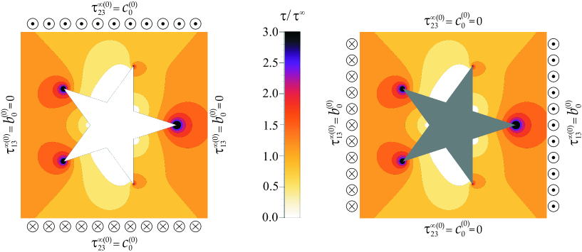
Figure 6: A five pointed star ($n=5$, $\xi=1/10$) polygonal void (left) is subject to a remote uniform antiplane shear (characterized by $c_{0}^{\text{\tiny\char 73}(0)}$ and $b_{0}^{\text{\tiny\char 73}(0)}$=0), while a rigid inclusion (right) is subject to the same remote shear field but rotated of $\pi/2$ (so that the remote stress field is characterized by $b_{0}^{\text{\tiny\char 72}(0)}=c_{0}^{\text{\tiny\char 73}(0)}$ and $c_{0}^{\text{\tiny\char 72}(0)}=0$). Under these conditions, the dimensionless shear stress fields ($\tau^{(0)}(x_{1},x_{2})/\tau^{\infty(0)}$) are identical for both the void and the rigid inclusion.

3.3 Shear stress analogies between rigid inclusions and voids

The purpose of this section is to highlight some special cases in which the stress fields generated within a matrix by a rigid inclusion are analogous to those generated when a void (of the same shape) is present.

Let us consider two remote stress fields of order $m$, equation (12), remotely applied to a matrix containing a void and a rigid inclusion (with the same shape) and which are defined respectively by the loading constants $b^{\text{\tiny\char 73}(m)}_{0},c^{\text{\tiny\char 73}(m)}_{0}$ and $b^{\text{\tiny\char 72}(m)}_{0},c^{\text{\tiny\char 72}(m)}_{0}$. From the obtained solution (73), if these constants satisfy the conditions

$$b^{\text{\tiny\char 73}(m)}_{0}=c^{\text{\tiny\char 72}(m)}_{0},\qquad b^{\text{\tiny\char 72}(m)}_{0}=-c^{\text{\tiny\char 73}(m)}_{0},$$ (76)

then the following shear stress analogy occurs

$$\tau_{13}^{\text{\tiny\char 73}(m)}\equiv\tau_{23}^{\text{\tiny\char 72}(m)},\qquad\tau_{23}^{\text{\tiny\char 73}(m)}\equiv-\tau_{13}^{\text{\tiny\char 72}(m)},$$ (77)

while, if the loading constants satisfy

$$b^{\text{\tiny\char 73}(m)}_{0}=-c^{\text{\tiny\char 72}(m)}_{0},\qquad b^{\text{\tiny\char 72}(m)}_{0}=c^{\text{\tiny\char 73}(m)}_{0},$$ (78)

then another shear stress analogy occurs

$$\tau_{13}^{\text{\tiny\char 73}(m)}\equiv-\tau_{23}^{\text{\tiny\char 72}(m)},\qquad\tau_{23}^{\text{\tiny\char 73}(m)}\equiv\tau_{13}^{\text{\tiny\char 72}(m)}.$$ (79)

Considering the above analogies, whenever the loading constants satisfy the conditions

$$\left|b^{\text{\tiny\char 73}(m)}_{0}\right|=\left|c^{\text{\tiny\char 72}(m)}_{0}\right|,\qquad\left|b^{\text{\tiny\char 72}(m)}_{0}\right|=\left|c^{\text{\tiny\char 73}(m)}_{0}\right|,\qquad b^{\text{\tiny\char 73}(m)}_{0}c^{\text{\tiny\char 73}(m)}_{0}=-b^{\text{\tiny\char 72}(m)}_{0}c^{\text{\tiny\char 72}(m)}_{0},$$ (80)

the modulus of the shear stress, equation (4), within the matrix generated by the void or by the inclusion are the same

$$\tau^{\text{\tiny\char 73}(m)}\equiv\tau^{\text{\tiny\char 72}(m)}.$$ (81)

An example of the identity of the fields of shear stress modulus generated by a void and a rigid inclusion under the conditions (80) is shown in Fig. 6 in the particular case of uniform remote stress, $m=0$.

4 Conclusions

Complex potentials and conformal mapping techniques have led to the analytical solution of isotoxal star-shaped polygonal voids and rigid inclusions (and also star-shaped cracks and stiffeners) subject to remote nonuniform antiplane shear loads. This solution will provide a guide for the development of numerical techniques in the presence of sharp corners and is important in the design of composite materials. The results pave the way to the discovery of situations in which the singularities (usually present at the inclusion vertices) disappear. This important issue is systematically addressed in Part II of this study.

References

- [1] Andersson, H., 1969. Stress-intensity factors at the tips of a star-shaped contour in an infinite tensile sheet. J. Mech. Phys. Solids 17, 5, 405-406.
- [2] Dal Corso, F., Shahzad, S., Bigoni D., 2016. Isotoxal star-shaped polygonal voids and rigid inclusions in nonuniform antiplane shear fields - II. Stress singularities, stress annihilation and inclusion invisibility. Int. J. Solids Structures , in press doi: 10.1016/j.ijsolstr.2016.01.026
- [3] Abramowitz, M., Stegun, I.A., 1972. Handbook of Mathematical Functions with Formulas, Graphs, and Mathematical Tables. Wiley–Interscience, NY.
- [4] Bacca, M., Dal Corso, F., Veber, D. and Bigoni, D., 2013. Anisotropic effective higher-order response of heterogeneous Cauchy elastic materials. Mech. Res. Comm., 54, 63-71.
- [5] Barbieri, E., Pugno, N.M., 2015. A computational model for large deformations of composites with a 2D soft matrix and 1D anticracks. Int. J. Solids Structures 77, 1-14.
- [6] Bigoni, D., Drugan, W.J., 2007. Analytical derivation of Cosserat moduli via homogenization of heterogeneous elastic materials. J. Appl. Mech. 74, 1-13.
- [7] Chen, J., 2012. Indentation-based methods to assess fracture toughness for thin coatings. J. Phys. D: Appl. Phys. 45, 203001.
- [8] Chen, F., Sevostianov, I., Girauda, A., Grgic, D., 2015. Evaluation of the effective elastic and conductive properties of a material containing concave pores. Int. J. Eng. Sci. , 97, 60 68.
- [9] Seagraves, A.N., Radovitzky, R.A., 2013. An analytical theory for Radial crack propagation: application to spherical indentation. J. Appl. Mech. 80, 1-5.
- [10] Rassoulova, N.B., 2010. The propagation of star-shaped brittle cracks. J. Appl. Mech. 77, 1-5.
- [11] Coxeter, H.S.M., 1989. Introduction to geometry. John Willey and Sons, NY.
- [12] Das, S.C., 1953. On the stresses due to a small spherical inclusion in a uniform beam under constant bending moment. Bull. Calcutta Math. Soc. 45, 55-63.
- [13] Eshelby, J.D., 1957. The Determination of the Elastic Field of an Ellipsoidal Inclusion and Related Problems. Proc. R. Soc. A 241, 376-396.
- [14] Gauthier, G., Lazarus, V., Pauchard, L., 2010. Shrinkage star-shaped cracks: Explaining the transition from 90 degrees to 120 degrees. EPL 89, 26002.
- [15] Gupta, M., Alderliesten, R.C., Benedictus, R., 2015. A review of T-stress and its effects in fracture mechanics. Eng. Fract. Mech. 134, 218-241.
- [16] Grunbaum, B., Shephard, G.C., 1987. Tilings and Patterns. W.H. Freeman and Company, NY.
- [17] Kohno, Y., Ishikawa, H., 1995. Singularities and stress intensities at the corner point of a polygonal hole and rigid polygonal inclusion under antiplane shear. Int. J. Eng. Sci. 33, 1547-1560.
- [18] Maurini, C., Bourdin, B., Gauthier, G., Lazarus, V., 2013. Crack patterns obtained by unidirectional drying of a colloidal suspension in a capillary tube: experiments and numerical simulations using a two-dimensional variational approach. Int. J. Fracture 184, 75-91.
- [19] Misseroni, D., Dal Corso, F., Shahzad, S., Bigoni, D., 2014. Stress concentration near stiff inclusions: Validation of rigid inclusion model and boundary layers by means of photoelasticity. Eng. Fract. Mech. 121-122, 87-97.
- [20] Noselli, G., Dal Corso, F. and Bigoni, D., 2010. The stress intensity near a stiffener disclosed by photoelasticity. Int. J. Fracture 166, 91-103.
- [21] Moon, H.J., Earmme, Y.Y., 1998. Calculation of elastic T-stresses near interface crack tip under in-plane and anti-plane loading. Int. J. Fracture 91, 179-195.
- [22] Radaj, D., 2013. State-of-the-art review on extended stress intensity factor concepts. Fatigue Fract. Eng. Mat. Str. 37, 1-28.
- [23] Movchan, A.B., Movchan, N.V., 1995. Mathematical Modelling of Solids with Nonregular Boundaries. CRC Press.
- [24] Movchan, A.B., Movchan, N.V., Poulton, C.G., 2002. Asymptotic Models of Fields in Dilute and Densely Packed Composites. Imperial College Press.
- [25] Muskhelishvili, N.I., 1953. Some Basic Problems of the Mathematical Theory of Elasticity. P. Nordhoff Ltd., Groningen.
- [26] Olver, F.W.J., Lozier, D.W., Boisvert, R.F., Clark, C.W., 2010. NIST Handbook of Mathematical Functions. Cambridge University Press, NY.
- [27] Piccolroaz, A., Mishuris, G., Movchan, A.B., 2010. Perturbation of Mode III interfacial cracks. Int. J. Fracture 166, 41-51.
- [28] Piccolroaz, A., Mishuris, G., Movchan, A.B., 2009. Symmetric and skew-symmetric weight functions in 2D perturbation models for semi-infinite interfacial cracks. J. Mech. Phys. Solids 57, 1657-1682.
- [29] Piccolroaz, A., Mishuris, G., Movchan, A., Movchan, N., 2012. Perturbation analysis of Mode III interfacial cracks advancing in a dilute heterogeneous material. Int. J. Solids Structures 49, 244-255.
- [30] Morini, L., Piccolroaz, A., Mishuris, G., Radi, E., 2013. Integral identities for a semi-infinite interfacial crack in anisotropic elastic bimaterials. Int. J. Solids Structures 50, 1437-1448.
- [31] Piccolroaz, A. and Mishuris, G., 2013. Integral identities for a semi-infinite interfacial crack in 2D and 3D elasticity. J. Elasticity , 110, 117-140.
- [32] Schiavone, P., 2003. Neutrality of the elliptic inhomogeneity in the case of non-uniform loading. Int. J. Eng. Sci. 8, 161-169.
- [33] Savin, G.N., 1961. Stress concentration around holes. Pergamon Press.
- [34] Sen, B., 1933. On the Concentration of Stresses Due to a Small Spherical Cavity in a Uniform Beam Bent by Terminal Couples. Bull. Calcutta Math. Soc. 25, 107-114.
- [35] Sih, G.C., 1965. Stress Distribution Near Internal Crack Tips for Longitudinal Shear Problems. J. Appl. Mech. 32, 51-58.
- [36] Seweryn, A., Molski, K., 1996. Elastic stress singularities and corresponding generalized stress intensity factors for angular corners under various boundary conditions. Eng. Fract. Mech. 55, 529-556.
- [37] Driscoll, T.A., Trefethen, L.N., 2002. Schwarz-Christoffel Mapping. Cambridge University Press.
- [38] Vandenberghe, N., Vermorel, R., Villermaux, E., 2013. Star-shaped crack pattern of broken windows. Phys. Rev. Letters 110, 174302.
- [39] Van Vliet, D., Schiavone, P., Mioduchowski, A., 2003. On the Design of Neutral Elastic Inhomogeneities in the Case of Non-Uniform Loading. Math. Mech. Solids 41, 2081-2090.
- [40] Vasudevan, M., Schiavone, P., 2006. New results concerning the identification of neutral inhomogeneities in plane elasticity. Arch. Mechanics 58, 45-58.