Tunable breakdown of the polaron picture for mobile impurities in a topological semimetal

Abstract

Mobile impurities in cold atomic gases constitute a new platform for investigating polaron physics. Here we show that when impurity atoms interact with a two-dimensional Fermi gas with quadratic band touching the polaron picture may either hold or break down depending on the particle-hole asymmetry of the band structure. If the hole band has a smaller effective mass than the particle band, the quasiparticle is stable and its diffusion coefficient varies with temperature as $D(T)\propto\ln^{2}T$. If the hole band has larger mass, the quasiparticle weight vanishes at low energies due to an emergent orthogonality catastrophe. In this case we map the problem onto a set of one-dimensional channels and use conformal field theory techniques to obtain $D(T)\propto T^{\nu}$ with an interaction-dependent exponent $\nu$. The different regimes can be detected in the nonequilibrium expansion dynamics of an initially confined impurity.

Introduction.—Recent experiments with mixtures of ultracold atoms have rekindled the interest in mobile impurities in quantum many-body systems Schirotzek et al. (2009); Palzer et al. (2009); Kohstall et al. (2012); Koschorreck et al. (2012); Spethmann et al. (2012); Fukuhara et al. (2013); Hu et al. (2016); Jørgensen et al. (2016). In these experiments, the mobile impurity is represented by an atom of a dilute species that interacts with collective excitations of a majority species, which can be either bosonic Cucchietti and Timmermans (2006); Bruderer et al. (2007); Tempere et al. (2009); Caracanhas, Bagnato, and Pereira (2013); Grusdt et al. (2015); Christensen, Levinsen, and Bruun (2015) or fermionic Chevy (2006); Combescot et al. (2007); Mathy, Parish, and Huse (2011); Schmidt et al. (2012); Massignan, Zaccanti, and Bruun (2014). In the latter case, the quasiparticle in the interacting system is called a Fermi polaron and is formed by an atom dressed by density fluctuations of the Fermi gas. The study of mobile impurities may lead to new techniques to probe strongly correlated states of matter Punk and Sachdev (2013); Grusdt et al. (2016). In addition, it allows us to reassess some fundamental questions about the formation of quasiparticles, while performing quantitative tests of existing theories Massignan, Zaccanti, and Bruun (2014); Christensen, Levinsen, and Bruun (2015).

On the other hand, it is natural to ask whether mobile impurities in cold atomic gases can also be used to investigate the breakdown of the quasiparticle picture. In fact, an outstanding problem in condensed matter physics pertains to the properties of phases without well-defined quasiparticles Senthil (2008); Witczak-Krempa, Sorensen, and Sachdev (2014); Hartnoll (2015), a famous example of which is the strange metal phase of hole-doped cuprates Lee, Nagaosa, and Wen (2006). Experience in this field has taught us that one route to the absence of quasiparticles (in the sense of vanishing quasiparticle weight Varma, Nussinov, and van Saarloos (2002)) is the coupling of a system to soft fluctuations near a quantum critical point Varma et al. (1989); Altshuler, Ioffe, and Millis (1994); Polchinski (1994); Nayak and Wilczek (1994).

In this work, we propose and analyze a mobile impurity model that can be driven between two regimes, in which the polaron picture either holds or breaks down, by varying a single parameter of a microscopic Hamiltonian. The main idea is to find a scale-invariant model where a marginal interaction gives rise to infrared singularities analogous to those in theories of non-Fermi liquids Varma, Nussinov, and van Saarloos (2002). For this purpose, we must couple the impurity with quadratic dispersion to an environment that also features quadratic dispersion at low energies. Indeed, the case of short-range interactions with linearly dispersing critical modes only involves strictly irrelevant perturbations of the free model Punk and Sachdev (2013). For this reason, we consider a two-dimensional (2D) Fermi gas with a quadratic band crossing point (QBCP) Sun et al. (2009); Uebelacker and Honerkamp (2011); Fu (2011); Sun et al. (2012); Tkachov (2013); Wang et al. (2015). This peculiar band touching can be protected by point group symmetries when it is associated with a nontrivial Berry flux, as in the checkerboard lattice Sun et al. (2009), thus characterizing a type of topological semimetal Sun et al. (2012). For free fermions, tuning the chemical potential to the QBCP leads to a low-energy spectrum of particle-hole pairs with quadratic dispersion. Remarkably, a repulsive interaction between fermions in the bulk is a marginally relevant perturbation that drives instabilities towards nematic or quantum Hall phases Sun et al. (2009); Uebelacker and Honerkamp (2011).

Our mobile impurity model can be viewed as the limit of extreme population imbalance of the model in Ref. Sun et al. (2009), in which a single spin-down fermion interacts with a finite density of spin-up fermions tuned to the QBCP. If the interaction is restricted to the $s$-wave channel, there is no direct interaction among spin-up fermions. In the following we show that the fate of the mobile impurity depends on the particle-hole asymmetry of the bulk fermion bands. In the regime where the filled band below the QBCP has a smaller effective mass than the empty band above it, the polaron is well defined, but the ratio between the decay rate and the energy vanishes only logarithmically in the low-energy limit. In the opposite regime, we find a divergent enhancement of the impurity mass and vanishing quasiparticle weight due to an emergent orthogonality catastrophe (OC) Anderson (1967); Knap et al. (2012); Mahan (2000); Gogolin, Nersesyan, and Tsvelik (2004). It is possible to switch between the two regimes by controlling hopping parameters in the optical lattice. Finally, we show that one can clearly distinguish between these regimes by measuring the diffusion coefficient in the expansion dynamics of an initially confined impurity. We stress that the exotic behavior discussed does not occur for an impurity immersed in a conventional 2D Fermi gas where the low-energy particle-hole pairs have linear dispersion about the Fermi surface Massignan, Zaccanti, and Bruun (2014).

Figure 1: (Color online) (a) Checkerboard lattice. Red sites belong to the A sublattice and green sites to the B sublattice. There is a hopping parameter $t$ (solid line) between nearest neighbors in different sublattices and direction-dependent hopping $t_{1}$ (dashed line) or $t_{2}$ (dotted line) between second neighbors. (b) Band structure for $t_{1}/t=0.7$ and $t_{2}/t=-0.3$, showing a QBCP in the regime $m_{+}<m_{-}$.

Model.—We consider the lattice model

$$H=\sum_{i,j}(t_{ij}c^{\dagger}_{i}c^{\phantom{\dagger}}_{j}+J_{ij}d^{\dagger}_{i}d^{\phantom{\dagger}}_{j})+U\sum_{i}c^{\dagger}_{i}c^{\phantom{\dagger}}_{i}d^{\dagger}_{i}d^{\phantom{\dagger}}_{i},$$ (1)

where $c_{j}$ annihilates a fermion of the majority species on site $j$ and $d_{j}$ annihilates the mobile impurity. The Hilbert space obeys the constraint $\sum_{j}d^{\dagger}_{j}d^{\phantom{\dagger}}_{j}=1$. The hopping parameters $t_{ij}$ and $J_{ij}$ are defined on a checkerboard lattice with sublattices A and B. For the $c$ fermions, we assign $t_{ij}$ as illustrated in Fig. 1(a) Fradkin (2013). For the impurity, we set $J_{ij}=rt_{ij}$, where $r$ is the parameter that controls the mass ratio, but the lattice is not crucial for the impurity. We can also consider a free-particle dispersion if the impurity does not couple to a species-specific lattice potential LeBlanc and Thywissen (2007). We note that optical checkerboard lattices have been realized experimentally Ölschläger et al. (2012); Windpassinger and Sengstock (2013). Finally, $U>0$ is the strength of the on-site repulsion, which is related to the interspecies $s$-wave scattering length Jaksch et al. (1998).

For $U=0$, the tight-binding Hamiltonian for the majority fermions can be diagonalized in the form $H_{0}=\sum_{i,j}t_{ij}c^{\dagger}_{i}c^{\phantom{\dagger}}_{j}=\sum_{\mathbf{k}}\Psi^{\dagger}_{\mathbf{k}}H_{0}(\mathbf{k})\Psi^{\phantom{\dagger}}_{\mathbf{k}}$, where $\Psi_{\mathbf{k}}=(a_{\mathbf{k}},b_{\mathbf{k}})^{t}$ is a two-component spinor and

$$H_{0}(\mathbf{k}) = 2t_{I}(\cos k_{x}+\cos k_{y})\mathbbm{1}+2t_{z}(\cos k_{x}-\cos k_{y})\sigma_{z}$$ (2)

$$+8t_{x}\cos(k_{x}/2)\cos(k_{y}/2)\sigma_{x},$$

with $t_{I}=(t_{1}+t_{2})/2$, $t_{z}=(t_{1}-t_{2})/2$, and $t_{x}=t/2$. Here the momentum $\mathbf{k}$ is in the Brillouin zone of the square lattice (with lattice parameter set to 1) and the Pauli matrices $\sigma_{l}$, $l\in\{x,y,z\}$, act in the internal sublattice space of $\Psi_{\mathbf{k}}$. For $t_{I}=0$, the Hamiltonian has a particle-hole symmetry $\mathcal{C}^{-1}H_{0}(\mathbf{k})\mathcal{C}=-H_{0}(\mathbf{k})$ with $\mathcal{C}=\sigma_{y}$.

We consider the fermion density at half-filling, $\langle c_{j}^{\dagger}c^{\phantom{\dagger}}_{j}\rangle=1/2$. At low energies, we expand the Hamiltonian about the band touching point $\mathbf{Q}=(\pi,\pi)$ and obtain ${H_{0}(\mathbf{Q}+\mathbf{p})}\approx{t_{I}(p_{x}^{2}+p_{y}^{2}-4)}\mathbbm{1}+t_{z}(p_{x}^{2}-p_{y}^{2})\sigma_{z}+2t_{x}p_{x}p_{y}\sigma_{x}$. Hereafter we restrict to $|t_{x}|=|t_{z}|$, in which case the model has continuous rotational invariance in the continuum limit Sun et al. (2009). The dispersion relation about the QBCP (dropping a constant) is given by $\varepsilon_{\pm}(\mathbf{p})=\pm p^{2}/(2m_{\pm})$, where $m_{+}$ ($m_{-}$) is the effective mass of particles (holes) in the upper (lower) band [see Fig. 1(b)]. In terms of the parameters in Eq. (2), $m_{\pm}=(t_{z}\pm t_{I})^{-1}$, where we assume $t_{z}>t_{I}\geq 0$. As expected, $m_{+}=m_{-}$ in the particle-hole symmetric case $t_{I}=0$, and the sign of $\Delta m=m_{+}-m_{-}$ can be controlled by varying $t_{I}$.

For the free impurity, we expand the Hamiltonian about the lowest-energy state at $\mathbf{k}=0$ and obtain the dispersion $E(\mathbf{p})\approx p^{2}/(2M)$. For $J_{ij}=rt_{ij}$, the free impurity mass is $M=[r(t_{z}-t_{I})]^{-1}$.

Turning on a weak interaction $U\ll t_{z}$, we obtain the mobile impurity model in the continuum limit

$$H_{\text{mob}} = \int d^{2}r\,\left[\Psi^{\dagger}(\mathbf{r})\mathcal{H}_{0}(\mathbf{r})\Psi(\mathbf{r})-\frac{1}{2M}d^{\dagger}(\mathbf{r})\nabla^{2}d^{\phantom{\dagger}}(\mathbf{r})\right.$$ (3)

$$\left.+2\pi\gamma\Psi^{\dagger}(\mathbf{r})\Psi(\mathbf{r})d^{\dagger}(\mathbf{r})d(\mathbf{r})\right],$$

where $\Psi(\mathbf{r})=(a(\mathbf{r}),b(\mathbf{r}))^{t}$ is the fermion field operator, $\mathcal{H}_{0}(\mathbf{r})=-t_{I}\nabla^{2}\mathbbm{1}-t_{z}[(\partial_{x}^{2}-\partial_{y}^{2})\sigma_{z}+2\partial_{x}\partial_{y}\sigma_{x}]$, and $\gamma\sim\mathcal{O}(U)$ is the coupling constant with units of inverse mass. The effective action corresponding to the Hamiltonian in Eq. (3) is scale invariant with dynamical exponent $z=2$ Sun et al. (2009); Fradkin (2013). A bosonic analogue of this model appears in the problem of a mobile impurity immersed in a Bose-Einstein condensate in a vortex-lattice state Caracanhas, Bagnato, and Pereira (2013); Caracanhas and Pereira (2015). An attempt to apply perturbation theory in $\gamma$ reveals logarithmic singularities reminiscent of the behavior in critical one-dimensional (1D) systems McGuire (1965); Castella and Zotos (1993); Kantian, Schollwöck, and Giamarchi (2014). This is a first sign of the peculiar effects of the marginal impurity-fermion interaction.

Low-energy fixed points.—We proceed with a perturbative renormalization group (RG) analysis of the interaction in Eq. (3). Computing the effective vertex and impurity self-energy to $\mathcal{O}(\gamma^{2})$, we obtain the set of RG equations

$$\frac{d\gamma}{d\ell} = \frac{\gamma^{2}(\mu_{-}-\mu_{+})Z}{4},$$ (4a)

$$\frac{dZ}{d\ell} = -\frac{\gamma^{2}\mu_{+}\mu_{-}Z}{2}\,F_{Z}\left(\frac{m_{+}}{M},\frac{m_{-}}{M}\right),$$ (4b)

$$\frac{dM}{d\ell} = \frac{\gamma^{2}(\mu_{+}\mu_{-})^{3/2}}{2}\,F_{M}\left(\frac{m_{+}}{M},\frac{m_{-}}{M}\right).$$ (4c)

Here $\ell=\ln(\Lambda_{0}/\Lambda)$, with $\Lambda$ the ultraviolet cutoff and $\Lambda_{0}\sim t_{z}$ the bare cutoff. The parameters $\mu_{\pm}=\left(\frac{1}{M}+\frac{1}{m_{\pm}}\right)^{-1}$ are reduced masses, $Z$ is the quasiparticle weight in the impurity Green’s function $G_{d}(\mathbf{p},\omega)\approx Z/[\omega-p^{2}/(2M)]$, and $F_{Z}(r_{+},r_{-})$ and $F_{M}(r_{+},r_{-})$, with $r_{\pm}=m_{\pm}/M$, are dimensionless functions of the mass ratios that can be determined numerically (see Supplemental Material sup ).

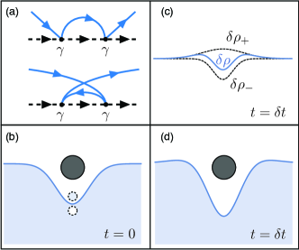
Figure 2: (Color online) Renormalization of the impurity-fermion interaction. (a) Diagrams that contribute at $\mathcal{O}(\gamma^{2})$. The solid line represents fermion propagators and the dashed line the impurity propagator. Panels (b)-(d) illustrate the mechanism. (b) For $\gamma>0$, the fermion density (blue shaded region) is depleted near the impurity. Conversely, the impurity experiences an effective potential that attracts it to the region of lower density. If the impurity is localized, the eigenstates of the Hamiltonian are the scattering states of a static potential. If the impurity mass is large but finite, the impurity can create particle-hole pairs as it moves slowly through the system. (c) For $m_{+}<m_{-}$, the particle wave packet (with density $\delta\rho_{+}$) will diffuse faster and have a larger width than the hole wave packet (with density $\delta\rho_{-}$) after some short time $\delta t$. The net density $\delta\rho=\delta\rho_{+}+\delta\rho_{-}$ is then a nonzero function of position with a minimum at the center. (d) This leads to a further depletion of the total density at the instantaneous position of the impurity and an enhancement of the effective potential. For $m_{+}>m_{-}$, the sign of $\delta\rho$ is reversed and the effective potential becomes shallower, implying that the interaction flows to weak coupling.

Remarkably, Eq. (4a) reveals that the coupling $\gamma>0$ can be relevant or irrelevant depending on particle-hole symmetry breaking. For $m_{+}=m_{-}$, the particle and hole diagrams that contribute to the renormalization of the interaction vertex at $\mathcal{O}(\gamma^{2})$, shown in Fig. 2(a), cancel exactly com . We have verified that this cancellation extends to higher orders in perturbation theory. Thus, in the particle-hole symmetric case the impurity-fermion interaction is strictly marginal.

For $m_{+}>m_{-}$, the interaction becomes marginally irrelevant. In this regime, the effective coupling at scale $\Lambda$ vanishes logarithmically, $\gamma(\Lambda)\sim 1/\ln(\Lambda_{0}/\Lambda)$, for $\Lambda\to 0$. Equations (4b) and (4c) imply that the impurity quasiparticle weight $Z(\Lambda)$ initially decreases and the effective mass $M(\Lambda)$ increases under the RG flow, but they both converge to finite values as $\gamma\to 0$. The picture for the low-energy fixed point is a Fermi polaron with renormalized $Z^{*}$ and $M^{*}$. In addition, the polaron has a finite decay rate because the single-particle dispersion is inside a continuum of particle-hole pairs and there is phase space for scattering at arbitrarily low energies Caracanhas, Bagnato, and Pereira (2013). On dimensional grounds, the decay rate for the polaron with momentum $\mathbf{p}$ is $1/\tau_{\mathbf{p}}\propto\gamma^{2}[E(\mathbf{p})]E(\mathbf{p})\propto p^{2}/\ln^{2}(p)$. Therefore, the quasiparticle is marginally stable as the ratio between the decay rate and the energy vanishes as $1/\ln^{2}(p)$ for $p\to 0$. Nonetheless, the impurity spectral function, which can be measured in cold atoms using rf spectroscopy Schirotzek et al. (2009); Shashi et al. (2014), must exhibit an approximately Lorentzian quasiparticle peak.

By contrast, the interaction is marginally relevant for $m_{+}<m_{-}$. The picture for the low-energy fixed point in this regime is the “self-trapping” of the impurity Caracanhas and Pereira (2015). As $M(\Lambda)$ grows without bound, we can analyze the RG equations for $M\gg m_{\pm}$ using $F_{Z}(r_{+},r_{-})\approx 1$ and $F_{M}(r_{+},r_{-})\approx\sqrt{\frac{r_{+}}{r_{-}}}+\sqrt{\frac{r_{-}}{r_{+}}}$ for $r_{\pm}\ll 1$. The result is that the effective mass diverges logarithmically, $M(\Lambda)\sim\ln(\Lambda_{0}/\Lambda)$, while the quasiparticle weight vanishes as a power law, $Z(\Lambda)\sim\Lambda^{g^{2}/2}$, where $g=\gamma^{*}(m_{+}m_{-})^{\frac{1}{2}}$ with $\gamma^{*}$ the renormalized coupling in the low-energy limit. Note that $\gamma(\Lambda)$ does not diverge for $\Lambda\to 0$ because its flow is slowed down by the suppression of $Z(\Lambda)$. This is the behavior expected from the OC for a localized impurity Anderson (1967); Knap et al. (2012); Mahan (2000); Gogolin, Nersesyan, and Tsvelik (2004). We stress that here the OC occurs in the absence of a Fermi surface. This is possible because the 2D QBCP has a finite density of states.

To demonstrate the OC explicitly, we analyze the vicinity of the infinite-mass fixed point. Neglecting the kinetic energy of the impurity (of order $M^{-1}$), we consider the Hamiltonian for the impurity localized at $\mathbf{r}=0$:

$$H_{\text{loc}}=\int d^{2}r\,\Psi^{\dagger}(\mathbf{r})[\mathcal{H}_{0}(\mathbf{r})+2\pi\gamma^{*}\delta(\mathbf{r})]\Psi(\mathbf{r}).$$ (5)

We use the partial wave expansion

$$\Psi^{\phantom{\dagger}}_{\lambda}(\mathbf{p})=\Psi^{\phantom{\dagger}}_{\lambda}(p,\theta_{\mathbf{p}})=\frac{1}{\sqrt{2\pi p}}\sum_{\ell\in\mathbb{Z}}e^{i\ell\theta_{\mathbf{p}}}\chi_{\lambda\ell}(p),$$ (6)

where $\lambda=\pm$ is the band index, $\theta_{\mathbf{p}}=\arctan(p_{y}/p_{x})$ is the polar angle of $\mathbf{p}$, and $\chi_{\lambda\ell}(p)$ obeys $\{\chi^{\phantom{\dagger}}_{\lambda\ell}(p),\chi^{\dagger}_{\lambda^{\prime}\ell^{\prime}}(k)\}=\delta_{\lambda,\lambda^{\prime}}\delta_{\ell,\ell^{\prime}}\delta(p-k)$. We then define the rescaled field $\psi_{\lambda,\ell}(\mathcal{K})=2\pi(m_{\lambda}/p)^{1/2}\chi_{\lambda,\ell}(p)$, where $\mathcal{K}=p^{2}/(8\pi^{2}m_{\lambda})$. This allows us to introduce a 1D chiral fermion for each $\ell$ channel by $\psi_{\ell}(x)=\int_{-\infty}^{+\infty}\frac{d\mathcal{K}}{\sqrt{2\pi}}\,e^{i\mathcal{K}x}[\theta(\mathcal{K})\psi_{+,\ell}(\mathcal{K})+i\text{sgn}(\ell)\theta(-\mathcal{K})\psi_{-,\ell}(-\mathcal{K})]$. We can then rewrite Eq. (5) in the form

$$H_{\text{loc}} = \sum_{\ell\in\mathbb{Z}}\int_{-\infty}^{\infty}dx\,\psi^{\dagger}_{\ell}(-i\partial_{x})\psi^{\phantom{\dagger}}_{\ell}$$ (7)

$$+\pi g[\psi^{\dagger}_{1}(0)\psi^{\phantom{\dagger}}_{1}(0)+\psi^{\dagger}_{-1}(0)\psi^{\phantom{\dagger}}_{-1}(0)].$$

Thus, only the $\ell=\pm 1$ channels couple to the impurity potential. This is due to the angular dependence of the eigenstates of $H_{0}$, which is also responsible for the nonzero Berry flux of the QBCP sup .

The Hamiltonian for $\ell=\pm 1$ channels in Eq. (7) has the standard form of a 1D conformal field theory with a boundary condition changing operator Schotte and Schotte (1969); Affleck and Ludwig (1994). The boundary term can be eliminated by a unitary transformation that changes the scaling dimension of various operators. We can then compute correlation functions by standard methods Gogolin, Nersesyan, and Tsvelik (2004). In particular, the impurity Green’s function has a power-law decay in time $|G_{d}(\mathbf{p}=0,t)|\propto t^{-g^{2}/2}$. In the frequency domain, the line shape of the spectral function becomes asymmetric, approaching a power-law singularity as $p\to 0$ Caracanhas and Pereira (2015). At finite $p$, the singularity is broadened at the energy scale $\sim g^{2}p^{2}/M[E(\mathbf{p})]$ due to the recoil of the heavy impurity Gavoret et al. (1969); Doniach (1970); Rosch (1999). The physical mechanism behind this low-energy fixed point can be understood within a simple cartoon picture in the limit $M\gg m_{\pm}$ as illustrated in Fig. 2.

Figure 3: (Color online) Sketch of the temperature dependence of the diffusion coefficient for $m_{+}>m_{-}$ (blue solid line) and $m_{+}<m_{-}$ (red dashed line). The dotted line indicates the scaling result $D(T)=\text{const.}$ expected at higher $T$.

Diffusion coefficient.—We now turn to transport, which can be induced and probed in cold atoms by controlling the trapping potential or artificial gauge fields Ott et al. (2004); Palzer et al. (2009); Schneider et al. (2012); Ronzheimer et al. (2013); Goldman et al. (2014); Chien, Peotta, and Di Ventra (2015). A particularly relevant response function is the temperature-dependent diffusion coefficient $D(T)$ Weiss (1999). Experimentally, one can measure the diffusion coefficient by preparing an initial state in which the impurity is confined by a trapping potential and watching the spreading of the wave packet after the trap is switched off Catani et al. (2012); Ronzheimer et al. (2013); Kindermann et al. (2016). After sufficiently long times, we expect diffusive expansion limited by inelastic collisions with the Fermi gas. The variance of the impurity position must then increase with time as $\sigma^{2}(t)=4D(T)t$. The diffusion coefficient is connected with the impurity mobility $\mu(T)$ via Einstein’s relation $D(T)=k_{B}T\mu(T)$ Weiss (1999).

For $m_{+}>m_{-}$, we calculate $D(T)$ in the linear response regime as $D(T)=k_{B}T\tau_{\text{tr}}/M_{0}$, where $M_{0}=M(\Lambda_{0})$ is the bare mass and $\tau_{\text{tr}}$ is the transport relaxation time of the long-lived quasiparticles. The transport relaxation time can be determined by a partial summation of diagrams in the Kubo formula for the mobility Langreth and Kadanoff (1964); Mahan (1966) or more simply using a memory function approach Götze and Wölfle (1972) to lowest order in $\gamma$. We find

$$D(T)\propto 1/\gamma^{2}(T)\propto\ln^{2}(\Lambda_{0}/T).$$ (8)

Note that from scaling we would expect $D(T)=\text{const.}$ since the diffusion is limited by a marginal interaction. The enhancement of $D(T)$ by the logarithmic correction in Eq. (8) is due to the flow of effective coupling constant to weak coupling as $T\to 0$.

For $m_{+}<m_{-}$, we can still use the memory function approach, which does not rely on the existence of quasiparticles. First, we employ the Lee-Low-Pines transformation Lee, Low, and Pines (1953); Grusdt and Demler (2015) to the frame comoving with the impurity and obtain the transformed Hamiltonian

$$\tilde{H}_{\text{mob}}=\frac{1}{2M}\left(\mathbf{P}+i\int d^{2}r\,\Psi^{\dagger}\nabla\Psi\right)^{2}+H_{\text{loc}},$$ (9)

where $\mathbf{P}$ is the total momentum of the system. The transformed impurity current operator is $\tilde{\mathbf{J}}_{d}=\frac{1}{M}\left(\mathbf{P}+i\int d^{2}r\,\Psi^{\dagger}\nabla\Psi\right)$. We also need the time derivative $\partial_{t}\tilde{\mathbf{J}}_{d}=-\frac{2\pi\gamma^{*}}{M}[\Psi^{\dagger}(0)\nabla\Psi(0)+\text{h.c.}]$. The mobility is calculated using $[\mu(T)]^{-1}=\frac{M^{2}}{\omega}\text{Im}[R_{\text{ret}}(\omega)-R_{\text{ret}}(0)]$. Here $R_{\text{ret}}(\omega)$ is the retarded memory function obtained from the imaginary-time correlation $R(\tau)=\langle\partial_{\tau}\tilde{\mathbf{J}}_{d}(\tau)\cdot\partial_{\tau}\tilde{\mathbf{J}}_{d}(0)\rangle$ by Fourier transform and an analytic continuation to real frequency. Importantly, the impurity mobility is determined by a local correlation function of the fermion field which can be calculated at the low-energy fixed point described by Eq. (7) (see Supplemental Material sup ). We find that for $m_{+}<m_{-}$ and $T\to 0$

$$D(T)\propto T^{\nu},\qquad\nu=1-\left(1-\frac{g}{2}\right)^{2}.$$ (10)

The anomalous dimension $\nu\sim\mathcal{O}(g)$ is analogous to the exponent of the Fermi edge singularity in metals Gogolin, Nersesyan, and Tsvelik (2004). In sharp contrast with Eq. (8), in this case $D(T)$ vanishes in the limit $T\to 0$. The result is depicted in Fig. 3.

We would like to emphasize that our work differs from previous studies of dissipative quantum dynamics where an impurity localization transition can be driven by varying the strength of the coupling to an Ohmic bath Fisher and Zwerger (1985); Weiss (1999). In that case, the impurity-bath coupling is strictly relevant or irrelevant. In our case, both regimes can be realized at weak coupling and are due to the effects of a marginal interaction. Note in particular that for $m_{+}<m_{-}$ the mobility diverges in the low-temperature limit as $\mu(T)\propto T^{-1+\nu}$, with $\nu$ governed by a marginal boundary operator.

Conclusion.—We have shown that mobile impurities coupled to a 2D Fermi gas with quadratic band touching exhibit anomalous single-particle and transport properties. Controlling the particle-hole asymmetry of the fermionic bands allows one to tune between a regime of well-defined quasiparticles and another regime where the quasiparticle weight vanishes due to an emergent orthogonality catastrophe. Experiments that probe the expansion dynamics of an impurity wave packet should observe a striking difference in the temperature dependence of the diffusion coefficient in these two regimes.

Appendix A Supplemental Material

A.1 1. Renormalization group equations

To derive the perturbative RG equations, we use the impurity Green’s function

$$G_{d}(k)=G_{d}(\mathbf{k},i\omega)=\frac{Z}{i\omega-E(\mathbf{k})}.$$ (11)

For the Fermi gas we define a matrix Green’s function

$$\mathbbm{G}=\left(\begin{array}[]{cc}\mathcal{G}_{11}&\mathcal{G}_{12}\\ \mathcal{G}_{21}&\mathcal{G}_{22}\end{array}\right),$$ (12)

with components

$$\mathcal{G}_{mn}(\mathbf{p},\tau)=-\langle T_{\tau}\Psi^{\phantom{\dagger}}_{m}(\mathbf{p},\tau)\Psi^{\dagger}_{n}(\mathbf{p},0)\rangle,$$ (13)

where $m,n\in\{1,2\}$ are sublattice indices with $\Psi_{1}(\mathbf{p})=a_{\mathbf{p}}$, $\Psi_{2}(\mathbf{p})=b_{\mathbf{p}}$. The orthogonal transformation that diagonalizes $H_{0}(\mathbf{p})$ in the continuum limit is $\Psi_{m}(\mathbf{p})=\sum_{\lambda}U_{m\lambda}(\mathbf{p})\Psi_{\lambda}(\mathbf{p})$, where $\lambda\in\{+,-\}$ is a band index, and

$$U(\mathbf{p})=U(\theta_{\mathbf{p}})=\left(\begin{array}[]{cc}\sin\theta_{\mathbf{p}}&\cos\theta_{\mathbf{p}}\\ -\cos\theta_{\mathbf{p}}&\sin\theta_{\mathbf{p}}\end{array}\right).$$ (14)

The RG equation for the effective coupling constant $\gamma(\Lambda)$ is obtained by considering the four-point function

$$\Pi(\{x_{i}\}) = -\sum_{n}\langle T_{\tau}\Psi^{\phantom{\dagger}}_{n}(x_{1})\Psi^{\dagger}_{n}(x_{2})d(x_{3})d^{\dagger}(x_{4})\rangle,$$ (15)

where $x_{i}=(\mathbf{r}_{i},\tau_{i})$, and its Fourier transform

$$\Pi(\{p_{i}\}) = \int\prod_{i=1}^{4}d^{2}r_{i}d\tau_{i}e^{i\omega_{i}\tau_{i}}e^{-i\mathbf{p}_{i}\cdot\mathbf{r}_{i}}\Pi(\{x_{i}\}).$$ (16)

The result is of the form

$$\Pi(\{p_{i}\}) = 2\pi\Gamma(\{p_{i}\})\text{Tr}\{\mathbbm{G}(p_{1})\mathbbm{G}(p_{2})\}G_{d}(p_{3})G_{d}(p_{4})$$ (17)

$$\times\delta_{\sum_{i}\mathbf{p}_{i},0}2\pi\delta\left(\sum_{i}\omega_{i}\right).$$

where $\Gamma(\{p_{i}\})$ is the effective vertex. At tree level, we have $\Gamma(\{p_{i}\})=\gamma$. The quantum correction at one-loop level is calculated using a cutoff scheme that integrates out large-momentum states in the shell $K^{\prime}<|\mathbf{k}|<K$, with $K^{\prime}=Ke^{-d\ell/2}$. Here we define $d\ell=d\Lambda/\Lambda=2dK/K$, where $\Lambda=K^{2}/2M_{0}$ is the energy cutoff that corresponds to the momentum cutoff $K$. The particle and hole diagrams in Fig. 2(a) of the main text yield

$$\Gamma^{(2)}_{\text{part}}(\{p_{i}\to 0\}) = -\frac{\mu_{+}\gamma^{2}Zd\ell}{4},$$

$$\Gamma^{(2)}_{\text{hole}}(\{p_{i}\to 0\}) = \frac{\mu_{-}\gamma^{2}Zd\ell}{4}.$$ (18)

This leads to the RG equation for $\gamma(\Lambda)$ in Eq. (4a).

To find the renormalization of the effective mass and quasiparticle weight, we calculate the two-loop “sunrise” diagram in the impurity self-energy at order $\gamma^{2}$, given by

$$\Sigma^{(2)}(\mathbf{p},i\omega) = -(2\pi\gamma)^{2}\sum_{\mathbf{k}}\sum_{\mathbf{q}}\int\frac{d\nu_{\mathbf{k}}}{2\pi}\int\frac{d\nu_{\mathbf{q}}}{2\pi}$$ (19)

$$\times\text{Tr}\{\mathbbm{G}(k+q)\mathbbm{G}(k)\}G_{d}(p-q).$$

The integration is performed such that both particle and hole momenta lie in the shell between $K^{\prime}$ and $K$. We are only interested in the result for small $\omega,p$. To lowest order in $p$ and $\omega$ the self-energy has the form

$$\Sigma^{(2)}(\mathbf{p},i\omega) \approx ia\omega-(a+b)\frac{p^{2}}{2M}.$$ (20)

We seek expressions for the coefficients $a$ and $b$, which determine the renormalized $M$ and $Z$ through $dZ=a$ and $dM=bM$. The result is

$$a = -\frac{\gamma^{2}\mu_{+}\mu_{-}}{2}F_{Z}\left(\frac{m_{+}}{M},\frac{m_{-}}{M}\right)d\ell,$$ (21)

$$b = \frac{\gamma^{2}(\mu_{+}\mu_{-})^{3/2}}{2M}F_{M}\left(\frac{m_{+}}{M},\frac{m_{-}}{M}\right)d\ell.$$ (22)

The functions of mass ratios are

$$F_{Z}\left(r_{+},r_{-}\right) = \int_{0}^{\pi/2}d\alpha\,\frac{(1+r_{+})(1+r_{-})}{r_{+}r_{-}\sin\alpha\cos\alpha}\left[\frac{\frac{1+r_{-}}{2r_{-}}\cos^{2}\alpha+\frac{1+r_{+}}{2r_{+}}\sin^{2}\alpha}{\sqrt{\left(\frac{1+r_{-}}{2r_{-}}\cos^{2}\alpha+\frac{1+r_{+}}{2r_{+}}\sin^{2}\alpha\right)^{2}-\sin^{2}\alpha\cos^{2}\alpha}}-1\right],$$ (23)

$$F_{M}(r_{+},r_{-}) = 2\int_{0}^{\pi/2}d\alpha\,\left[\frac{(1+r_{+})(1+r_{-})}{r_{+}r_{-}}\right]^{3/2}\frac{1-\sin(2\alpha)[3L+2(L^{2}-1)^{3/2}-2L^{3}]}{\sin^{2}(2\alpha)(L^{2}-1)^{3/2}},$$ (24)

where

$$L(\alpha,r_{+},r_{-})=\frac{\frac{1+r_{+}}{r_{+}}\sin^{2}\alpha+\frac{1+r_{-}}{r_{-}}\cos^{2}\alpha}{\sin(2\alpha)}.$$ (25)

The functions $F_{Z}(r_{+},r_{-})$ and $F_{M}(r_{+},r_{-})$ are illustrated in Fig. 4. Note that they are smooth functions of the mass ratios with values of order 1.

Figure 4: The functions of mass ratios that appear in the RG equations for $M(\Lambda)$ and $Z(\Lambda)$.

Appendix B 2. Mapping onto 1D chiral fermions

Using the partial wave expansion in Eq. (6) of the main text, we can write the free fermion model in the form

$$H_{0} = \sum_{\lambda=\pm}\int\frac{d^{2}p}{(2\pi)^{2}}\,\frac{\lambda p^{2}}{2m_{\lambda}}\Psi^{\dagger}_{\lambda}(\mathbf{p})\Psi^{\phantom{\dagger}}_{\lambda}(\mathbf{p})$$ (26)

$$= \sum_{\lambda,\ell}\frac{\lambda}{8\pi^{2}m_{\lambda}}\int_{0}^{\infty}dp\,p^{2}\chi^{\dagger}_{\lambda,\ell}(p)\chi^{\phantom{\dagger}}_{\lambda,\ell}(p).$$

Performing the change of variable to $\mathcal{K}=p^{2}/(8\pi^{2}m_{\lambda})$ and switching to the rescaled fields $\psi_{\lambda,\ell}(\mathcal{K})$, we obtain

$$H_{0} = \sum_{\lambda,\ell}\lambda\int_{0}^{\infty}d\mathcal{K}\,\mathcal{K}\psi^{\dagger}_{\lambda,\ell}(\mathcal{K})\psi^{\phantom{\dagger}}_{\lambda,\ell}(\mathcal{K})$$ (27)

$$= \sum_{\ell}\int_{-\infty}^{\infty}d\mathcal{K}\,\mathcal{K}\psi^{\dagger}_{\ell}(\mathcal{K})\psi^{\phantom{\dagger}}_{\ell}(\mathcal{K}),$$

where $\psi_{\ell}(\mathcal{K})\equiv\theta(\mathcal{K})\psi_{+,\ell}(\mathcal{K})+i\text{sgn}(\ell)\theta(-\mathcal{K})\psi_{-,\ell}(-\mathcal{K})$. The chiral fermion in “real” space is the Fourier transform

$$\psi_{\ell}(x)=\frac{1}{\sqrt{2\pi}}\int_{-\infty}^{\infty}d\mathcal{K}\,e^{i\mathcal{K}x}\psi_{\ell}(\mathcal{K}).$$ (28)

The potential scattering associated with the impurity at the origin can be written as

$$H_{\text{int}}=2\pi\gamma^{*}\sum_{\lambda,\mu}\int\frac{d^{2}k}{(2\pi)^{2}}\int\frac{d^{2}p}{(2\pi)^{2}}V^{\lambda,\mu}_{\mathbf{k},\mathbf{p}}\Psi^{\dagger}_{\lambda}(\mathbf{k})\Psi^{\phantom{\dagger}}_{\mu}(\mathbf{p}),$$ (29)

where $V^{\lambda,\mu}_{\mathbf{k},\mathbf{p}}=[U^{\dagger}(\mathbf{k})U(\mathbf{p})]_{\lambda\mu}$. From Eq. (14), we see that the amplitude $V^{\lambda,\mu}_{\mathbf{k},\mathbf{p}}$ only depends on the polar angles of $\mathbf{k}$ and $\mathbf{p}$. Written as a matrix in the band basis:

$$V_{\mathbf{k},\mathbf{p}}=\left(\begin{array}[]{cc}\cos(\theta_{\mathbf{k}}-\theta_{\mathbf{p}})&\sin(\theta_{\mathbf{k}}-\theta_{\mathbf{p}})\\ -\sin(\theta_{\mathbf{k}}-\theta_{\mathbf{p}})&\cos(\theta_{\mathbf{k}}-\theta_{\mathbf{p}})\end{array}\right).$$ (30)

Substituting the partial wave expansion into Eq. (29), we obtain

$$H_{\text{int}} = \frac{\gamma^{*}}{2\pi}\sum_{\lambda,\mu}\int_{0}^{\infty}dk\,k\int_{0}^{\infty}dp\,p\int_{-\pi}^{\pi}\frac{d\theta_{\mathbf{p}}}{2\pi}\int_{-\pi}^{\pi}\frac{d\theta_{\mathbf{k}}}{2\pi}$$ (31)

$$\times V^{\lambda,\mu}_{\mathbf{k},\mathbf{p}}\sum_{\ell,\ell^{\prime}}\frac{e^{i(\ell\theta_{\mathbf{p}}-\ell^{\prime}\theta_{\mathbf{k}})}}{2\pi\sqrt{pk}}\,\chi^{\dagger}_{\lambda,\ell}(k)\chi^{\phantom{\dagger}}_{\mu,\ell^{\prime}}(p)$$

$$= \frac{g}{2}\int_{0}^{\infty}d\mathcal{K}\int_{0}^{\infty}d\mathcal{K}^{\prime}\,\left[w^{\frac{1}{2}}\psi^{\dagger}_{1}(\mathcal{K})\psi^{\phantom{\dagger}}_{1}(\mathcal{K}^{\prime})\right.$$

$$+w^{-\frac{1}{2}}\psi^{\dagger}_{1}(-\mathcal{K})\psi^{\phantom{\dagger}}_{1}(-\mathcal{K}^{\prime})+\psi^{\dagger}_{1}(\mathcal{K})\psi^{\phantom{\dagger}}_{1}(-\mathcal{K}^{\prime})$$

$$\left.+\psi^{\dagger}_{1}(-\mathcal{K})\psi^{\phantom{\dagger}}_{1}(\mathcal{K}^{\prime})+(1\to-1)\right],$$

where $w=m_{+}/m_{-}$. We separate two terms $H_{\text{int}}=H_{\text{int}}^{(s)}+H_{\text{int}}^{(a)}$ with

$$H_{\text{int}}^{(s)} = \frac{g}{2}\int_{-\infty}^{\infty}d\mathcal{K}\int_{-\infty}^{\infty}d\mathcal{K}^{\prime}\,\left[\psi^{\dagger}_{1}(\mathcal{K})\psi^{\phantom{\dagger}}_{1}(\mathcal{K}^{\prime})\right.$$ (32)

$$\left.+(1\to-1)\right],$$

$$H_{\text{int}}^{(a)} = \int_{0}^{\infty}d\mathcal{K}\int_{0}^{\infty}d\mathcal{K}^{\prime}\,\left[\kappa_{+}\psi^{\dagger}_{1}(\mathcal{K})\psi^{\phantom{\dagger}}_{1}(\mathcal{K}^{\prime})\right.$$ (33)

$$\left.+\kappa_{-}\psi^{\dagger}_{1}(-\mathcal{K})\psi^{\phantom{\dagger}}_{1}(-\mathcal{K}^{\prime})+(1\to-1)\right],$$

where $\kappa_{+}\equiv(w^{\frac{1}{2}}-1)g/2$ and $\kappa_{-}\equiv(w^{-\frac{1}{2}}-1)g/2$. The term $H_{\text{int}}^{(s)}$ is the usual potential scattering and is local in the real 1D space

$$H_{\text{int}}^{(s)}=\pi g[\psi^{\dagger}_{1}(0)\psi^{\phantom{\dagger}}_{1}(0)+\psi^{\dagger}_{-1}(0)\psi^{\phantom{\dagger}}_{-1}(0)].$$ (34)

The term $H_{\text{int}}^{(a)}$ is due to the asymmetry between particle-to-particle versus hole-to-hole scattering processes. We can show that this term is irrelevant in the RG sense. In terms of the chiral fermions, we write

$$H_{\text{int}}^{(a)} = \frac{\kappa_{+}}{2\pi}\int dx_{1}dx_{2}\,\frac{\psi_{1}^{\dagger}(x_{1})\psi^{\phantom{\dagger}}_{1}(x_{2})}{(x_{1}+i\eta)(x_{2}-i\eta)}$$ (35)

$$+\frac{\kappa_{-}}{2\pi}\int dx_{1}dx_{2}\,\frac{\psi_{1}^{\dagger}(x_{1})\psi^{\phantom{\dagger}}_{1}(x_{2})}{(x_{1}-i\eta)(x_{2}+i\eta)}$$

$$+(1\to-1).$$

We employ Eq. (35) to work out the renormalization using the operator product expansion of the fermion fields in real space. The imaginary parts with $\eta\to 0^{+}$ control the positions of poles in the integrations over Euclidean spacetime. This way we obtain the RG equations to second order in $\kappa_{\pm}$

$$\frac{d\kappa_{+}}{d\ell}=\kappa_{+}^{2},\qquad\frac{d\kappa_{-}}{d\ell}=-\kappa_{-}^{2}.$$ (36)

Note that $\kappa_{+}<0$ and $\kappa_{-}>0$ since $w<1$ in the regime $m_{+}<m_{-}$. Thus, the particle-hole asymmetry in the potential scattering is irrelevant. However, like other irrelevant perturbations, $H_{\text{int}}^{(a)}$ may renormalize the scattering amplitude $g$ at the low-energy fixed point. This effect can be accounted for if we replace the weak coupling expression $g=\gamma^{*}\sqrt{m_{+}m_{-}}$ (valid to first order in $\gamma^{*}$) by the relation $g=\delta/\pi$, where $\delta$ is the exact phase shift of the potential, as in the usual OC Gogolin, Nersesyan, and Tsvelik (2004). Dropping $H_{\text{int}}^{(a)}$, we obtain the Hamiltonian in Eq. (7) of the main text.

Appendix C 3. Correlations in the regime $m_{+}<m_{-}$

We bosonize the chiral fermions in the form

$$\psi^{\phantom{\dagger}}_{\ell}(x)\sim e^{-i\sqrt{2\pi}\varphi_{\ell}(x)},$$ (37)

where $\varphi_{\ell}(x)$ is a chiral bosonic field that obeys $[\varphi_{\ell}(x),\partial_{r}\varphi_{\ell^{\prime}}(x^{\prime})]=-i\delta_{\ell,\ell^{\prime}}\delta(x-x^{\prime})$. The bosonized version of the Hamiltonian in Eq. (7) of the main text reads

$$H_{\text{loc}} = \sum_{\ell\in\mathbb{Z}}\frac{1}{2}\int_{-\infty}^{+\infty}dx\,(\partial_{x}\varphi_{\ell})^{2}$$ (38)

$$-g\sqrt{\frac{\pi}{2}}[\partial_{x}\varphi_{1}(0)+\partial_{x}\varphi_{-1}(0)].$$

We can eliminate the boundary operator by performing a unitary transformation

$$U=\exp\left\{-ig\sqrt{\frac{\pi}{2}}[\varphi_{1}(0)+\varphi_{-1}(0)]\right\},$$ (39)

which acts as

$$\tilde{H}_{\text{loc}}=U^{\dagger}H_{\text{loc}}U=\sum_{\ell}\frac{1}{2}\int_{-\infty}^{+\infty}dx\,(\partial_{x}\varphi_{\ell})^{2}=H_{0}.$$ (40)

The decay of the impurity Green’s function is due to the OC when we change the boundary condition in the $\ell=\pm 1$ channels. Let us denote the ground state of $H$ (in the presence of the impurity) as $|\tilde{0}\rangle=U|0\rangle$, where $|0\rangle$ is the ground state of $H_{0}$. Following Ref. Affleck and Ludwig, 1994, we write the impurity Green’s function as

$$\langle d(t)d^{\dagger}(0)\rangle = \langle 0|U(t)U^{\dagger}(0)|0\rangle.$$ (41)

This is a correlation function of the vertex operator in Eq. (39) evolved with the noninteracting Hamiltonian $H_{0}$. Normal ordering the exponentials and using the Baker-Hausdorff formula $e^{A}e^{B}=e^{B}e^{A}e^{[A,B]}$ we obtain

$$\langle d(t)d^{\dagger}(0)\rangle\propto t^{-g^{2}/2}.$$ (42)

To calculate the mobility, first we have to account for the finite mass of the impurity before we set up the calculation of the correlation function at the low-energy fixed point. The physical picture here is that when the impurity is very heavy the particle-hole excitations in the Fermi gas can follow its motion adiabatically. Thus, it is convenient to transform to the impurity frame and then determine the current decay through the correlation of the cloud that dresses the impurity.

We rewrite the time derivative of the current operator in the impurity frame in terms of chiral fermions:

$$\partial_{t}\tilde{\mathbf{J}}_{d} = -\frac{2\pi\gamma^{*}}{M}[\Psi^{\dagger}(0)\nabla\Psi(0)+\text{h.c.}]$$ (43)

$$= -\frac{i\gamma^{*}}{2\pi M}\sum_{\lambda}\int d^{2}k\int d^{2}p\,\mathbf{p}\Psi^{\dagger}_{\lambda}(\mathbf{k})\Psi^{\phantom{\dagger}}_{\lambda}(\mathbf{p})+\text{h.c.}$$

$$= -\frac{i8\pi^{4}\gamma^{*}}{M}\sum_{\lambda}(2m^{3}_{\lambda})^{1/2}\int_{0}^{\infty}d\mathcal{K}\int_{0}^{\infty}d\mathcal{K}^{\prime}\,$$

$$\times\sqrt{\mathcal{K}^{\prime}}\psi^{\dagger}_{\lambda,0}(\mathcal{K})\psi^{\phantom{\dagger}}_{\lambda,1}(\mathcal{K}^{\prime})+(1\to-1)+\text{h.c.}.$$

Note that the operator now transfer fermions between $\ell=0$ and $\ell=\pm 1$ channels.

Let us consider the correlation in imaginary time

$$R(\tau)=\langle\partial_{t}\tilde{\mathbf{J}}_{d}(\tau)\cdot\partial_{t}\tilde{\mathbf{J}}_{d}(0)\rangle.$$ (44)

We can calculate the correlation at zero temperature and later obtain the finite-temperature result using a conformal mapping. At zero temperature, $R(\tau)$ decays as a power law with an exponent determined by the scaling dimension of the operator $\partial_{t}\tilde{\mathbf{J}}_{d}$. Since we are only interested in the exponent and not on the prefactor, let us focus on the contribution from $\ell=1$

$$R(\tau) \sim R_{0}(\tau)R_{1}(\tau),$$ (45)

where we used the decoupling of $\ell=0$ and $\ell=1$ channels to factorize the correlation into

$$R_{0}(\tau) = \int_{0}^{\infty}d\mathcal{K}_{1}\int_{0}^{\infty}d\mathcal{K}_{2}\,\langle\psi^{\phantom{\dagger}}_{0}(\mathcal{K}_{1},\tau)\psi^{\dagger}_{0}(\mathcal{K}_{2},0)\rangle,$$ (46)

$$R_{1}(\tau) = \int_{0}^{\infty}d\mathcal{K}_{1}\int_{0}^{\infty}d\mathcal{K}_{2}\,\sqrt{\mathcal{K}_{1}\mathcal{K}_{2}}$$ (47)

$$\times\langle\psi^{\dagger}_{1}(\mathcal{K}_{1},\tau)\psi^{\phantom{\dagger}}_{1}(\mathcal{K}_{2},0)\rangle.$$

The $\ell=0$ channel is free and $\psi_{0}(x)$ has scaling dimension $1/2$. Thus, it is easy to check that $R_{0}(\tau)\sim 1/\tau$. For the $\ell=1$ channel, the correlation is affected by the boundary operator. The dominant long-time decay stems from the vicinity of $x=0$ and can be written in the form

$$R_{1}(\tau)\sim\frac{1}{\tau}\langle\psi^{\dagger}_{1}(0,\tau)\psi^{\phantom{\dagger}}_{1}(0,0)\rangle.$$ (48)

This correlation for the fermion field is analogous to that in the optical absorption rate in the x-ray edge problem Gogolin, Nersesyan, and Tsvelik (2004). Unlike the impurity Green’s function, in this case the correlation decays more slowly when we turn on the potential with $g>0$. We have

$$\langle\psi^{\dagger}_{1}(0,\tau)\psi^{\phantom{\dagger}}_{1}(0,0)\rangle = \langle 0|e^{H_{0}\tau}\tilde{\psi}^{\dagger}_{1}(0)e^{-H_{0}\tau}\tilde{\psi}^{\phantom{\dagger}}_{1}(0)|0\rangle,$$ (49)

where the transformed field

$$\tilde{\psi}_{1}(0)\sim e^{-i\sqrt{2\pi}(1-g/2)\varphi_{1}(0)}$$ (50)

has scaling dimension $(1-g/2)^{2}/2$. As a result, the correlation decays as

$$\langle\psi^{\dagger}_{1}(0,\tau)\psi^{\phantom{\dagger}}_{1}(0,0)\rangle\sim\tau^{-1+\nu},$$ (51)

with $\nu=1-(1-g/2)^{2}=g-g^{2}/4$.

Putting everything together, the correlation in Eq. (44) at zero temperature decays as

$$R(\tau)\sim\tau^{-3+\nu}.$$ (52)

Mapping to finite temperature and real time, we obtain

$$\text{Im}R_{\text{ret}}(\omega) \sim \int_{0}^{\infty}dt\,e^{i\omega t}\left[\frac{\pi T}{\sinh(\pi Tt)}\right]^{3-\nu}$$ (53)

$$\sim T^{2-\nu}B\left(\frac{3-\nu}{2}-\frac{i\omega}{2\pi T},\nu-2\right),$$

where $B(x,y)$ is Euler’s beta function. Since we are interested in the dc limit, we expand the beta function for small $\omega$ and obtain

$$\text{Im}R_{\text{ret}}(\omega)\sim\omega T^{1-\nu}.$$ (54)

This leads to the result for the mobility $\mu(T)\propto T^{-1+\nu}$ and for the diffusion coefficient $D(T)\propto T^{\nu}$.