Electromagnetic Casimir densities for a cylindrical
shell on de Sitter space

Abstract

Complete set of cylindrical modes is constructed for the electromagnetic field inside and outside a cylindrical shell in the background of $(D+1)$-dimensional dS spacetime. On the shell, the field obeys the generalized perfect conductor boundary condition. For the Bunch-Davies vacuum state, we evaluate the expectation values (VEVs) of the electric field squared and of the energy-momentum tensor. The shell-induced contributions are explicitly extracted. In this way, for points away from the shell, the renormalization is reduced to the one for the VEVs in the boundary-free dS bulk. As a special case, the VEVs are obtained for a cylindrical shell in the $(D+1)$-dimensional Minkowski bulk. We show that the shell-induced contribution in the electric field squared is positive for both the interior and exterior regions. The corresponding Casimir-Polder forces are directed toward the shell. The vacuum energy-momentum tensor, in addition to the diagonal components, has a nonzero off-diagonal component corresponding to the energy flux along the direction normal to the shell. This flux is directed from the shell in both the exterior and interior regions. For points near the shell, the leading terms in the asymptotic expansions for the electric field squared and diagonal components of the energy-momentum tensor are obtained from the corresponding expressions in the Minkowski bulk replacing the distance from the shell by the proper distance in the dS bulk. The influence of the gravitational field on the local characteristics of the vacuum is essential at distances from the shell larger than the dS curvature radius. The results are extended for confining boundary conditions of flux tube models in QCD.

PACS numbers: 04.62.+v, 03.70.+k, 11.10.Kk

1 Introduction

The Casimir effect (for reviews see [1]) is among the most interesting boundary-induced effects in quantum field theory. Nearly seventy years after its discovery, the effect continues to be area of active theoretical and experimental research today. This is due to of fundamental and practical importance of the Casimir effect in various fields of modern physics and technology. The imposition of boundary conditions on a quantum field shifts the expectation values of physical observables. The particular features of the effect depend on the spin of the field, on the geometries of boundaries and background spacetime, and on the specific boundary conditions. An interesting topic in the investigations of the Casimir effect is the dependence of the physical characteristics, such as the vacuum energy and forces acting on the boundaries, on the dimension of the background spacetime. In particular, this is motivated by the role of the Casimir effect in higher-dimensional models. The dependence of the Casimir energy on the size of the extra dimensions provides a mechanism for their stabilization. The latter is an important issue in both the Kaluza-Klein-type and braneworld models. In addition, the Casimir energy related to extra dimensions can serve as a model of dark energy driving the accelerating expansion of the Universe at recent epoch.

In the present paper we investigate combined effects of boundaries and background geometry on the local characteristics of the electromagnetic vacuum in an arbitrary number of spatial dimensions. As a background spacetime we consider $(D+1)$-dimensional de Sitter (dS) spacetime. This choice is motivated by several reasons. The dS spacetime has maximal number of symmetries and because of this a large number of physical problems can be solved exactly on its background. A better understanding of the influence of classical gravitational field on quantum matter in dS spacetime serves as a way to deal with less symmetric geometries. The quantum effects in dS bulk play an important role in inflationary scenarios (see [2] and [3] for recent reviews). Quantum fluctuations in the inflationary universe with dS geometry produce observable effects in the form of small density perturbations in the post-inflationary stage. These perturbations have nearly scale-invariant spectrum and form the base of the currently most popular mechanism for the generation of the seeds for galaxy formation. The corresponding predictions are in good agreement with the recent observational data on the temperature anisotropies of the cosmic microwave background radiation. The importance of dS spacetime as a gravitational background further increased after the discovery of the accelerating expansion of the Universe at recent epoch [4, 5]. Within the framework of general relativity, among the most popular cosmological models is the one with a positive cosmological constant as a driving source behind the accelerating expansion. In this model the dS spacetime is the future attractor for the geometry of our universe.

An important ingredient in the problems of the Casimir effect is the geometry of boundaries. Here we consider a cylindrical shell in background of dS spacetime, described by inflationary coordinates. On the shell the electromagnetic field obeys the generalized perfect conductor boundary condition. Along with the boundaries of planar and spherical symmetry, the cylindrical boundaries are among the most popular geometries in the investigations of the Casimir effect (see [1] and references therein). The patch of dS spacetime covered by inflationary coordinates is conformally flat and the corresponding results for the Casimir effect in the case of conformally invariant fields are obtained from the expressions for the Minkowski bulk by using the standard conformal relation between two problems (see, for instance, [6]). In particular, this is the case for the electromagnetic field in 4-dimensional spacetime. The case of conformally coupled massless scalar field obeying Dirichlet boundary condition on a spherical shell in 4-dimensional dS spacetime has been considered in [7].

For conformally non-invariant fields the investigation of the Casimir effect in dS spacetime requires a separate consideration. In this case, at distances from the boundaries larger than the curvature radius of the background spacetime, the influence of the gravitational field may lead to a behavior of the local characteristics of the vacuum essentially different from that in the Minkowski bulk. The scalar Casimir effect for a massive field with general curvature coupling and with Robin boundary conditions on planar boundaries in the background of $(D+1)$-dimensional dS spacetime has been investigated in [8]. The corresponding problem with a spherical boundary was discussed in [9]. An important feature for conformally non-invariant fields is that the vacuum energy-momentum tensor, in addition to the diagonal components, acquires an off-diagonal component corresponding to the energy flux along the direction normal to the boundary. The Casimir densities induced by a spherical dS bubble in the Minkowski bulk has been studied in [10]. For a scalar field, the geometry with a cylindrical boundary with Robin boundary condition was discussed in [11]. Depending on the mass of the field, at distances from the boundaries larger than the dS curvature radius, two different regimes are realized with monotonic or oscillatory decay of the vacuum expectation values. The electromagnetic Casimir effect for planar boundaries with generalized perfect conductor boundary conditions in dS bulk, having an arbitrary number of spatial dimensions, has recently been studied in [12] (for the propagators of vector fields on dS background in the absence of boundaries see [13]). The background geometry of Friedmann-Robertson-Walker cosmologies with power-law scale factors was discussed in [14].

The organization of the paper is the following. In the next section we consider the complete set of cylindrical modes for the electromagnetic field in dS spacetime, obeying the generalized perfect conductor boundary condition on a cylindrical shell. By using these modes, in section 3, the vacuum expectation value (VEV) of the electric field squared inside the shell is evaluated. Various asymptotic regions of the parameters are discussed. The VEV of the energy-momentum tensor is studied in section 4. The VEVs of the electric field squared and of the energy-momentum tensor in the exterior region are investigated in section 5. Section 6 summarizes the main results of the paper. In appendix A the cylindrical modes in $(D+1)$-dimensional Minkowski spacetime are discussed. The integrals, appearing in the expressions for the VEVs for the special case $D=4$, are evaluated in appendix B. In the numerical evaluations of the VEVs we have considered this special case.

2 Electromagnetic field modes in dS spacetime

We consider a quantum electromagnetic field in background of a $(D+1)$-dimensional dS spacetime, in the presence of a perfectly conducting cylindrical shell having the radius $a$. In accordance with the problem symmetry, we write the dS line element in cylindrical coordinates $\left(r,\phi,\mathbf{z}\right)$:

$$ds^{2}=dt^{2}-e^{2t/\alpha}\left[dr^{2}+r^{2}d\phi^{2}+\left(d\mathbf{z}\right)^{2}\right],$$ (2.1)

where $\mathbf{z=}\left(z^{3},...,z^{D}\right)$. The parameter $\alpha$ is expressed in terms of the cosmological constant $\Lambda$ through the relation $\alpha^{2}=D(D-1)/(2\Lambda)$. Below, in addition to the synchronous time coordinate $t$ we will use the conformal time $\tau$, defined as $\tau=-\alpha e^{-t/\alpha},\ -\infty<\tau<0$. In terms of this coordinate the metric tensor takes a conformally flat form $g_{\mu\nu}=(\alpha/\tau)^{2}g_{(\mathrm{M})\mu\nu}$, where $g_{(\mathrm{M})\mu\nu}=\mathrm{diag}(1,-1,-r^{2},-1,\ldots,-1)$ is the Minkowskian metric tensor.

We are interested in the changes of the VEVs for the electromagnetic field induced by a cylindrical boundary $r=a$ in the background of the geometry given by (2.1). In the canonical quantization procedure a complete orthonormal set of solutions to the classical field equations is required and, in this section, we present this set for the geometry at hand. For a free electromagnetic field the Maxwell equations have the form

$$\frac{1}{\sqrt{|g|}}\partial_{\nu}\left(\sqrt{|g|}F^{\mu\nu}\right)=0,$$ (2.2)

where $F_{\mu\nu}$ is the electromagnetic field tensor, $F_{\mu\nu}=\partial_{\mu}A_{\nu}-\partial_{\nu}A_{\mu}$. We assume that on the surface $r=a$ the field obeys the boundary condition

$$n^{\nu_{1}}\,{}^{\ast}F_{\nu_{1}\cdots\nu_{D-1}}=0,$$ (2.3)

where $n^{v}$ is the normal to the boundary, ${}^{\ast}F_{\nu_{1}\cdots\nu_{D-1}}$ is the dual of the field tensor $F_{\mu\nu}$. For $D=3$ the condition (2.3) reduces to the boundary condition on the surface of a perfect conductor. We want to find the complete set of solutions to the equation (2.2) in the coordinates $(\tau,r,\phi,\mathbf{z})$.

In the Coulomb gauge one has $A_{0}=0$, $\partial_{l}(\sqrt{|g|}A^{l})=0$, $l=1,...,D$. For the geometry under consideration the latter equation is reduced to

$$\sum_{l=1}^{D}\partial_{l}(rA^{l})=0,$$ (2.4)

which is the same as that in the Minkowski spacetime. If we present the solution in the factorized form, $A_{\mu}(\tau,x^{l})=T(\tau)S_{\mu}(x^{l})$, then it can be shown that the parts of the mode functions corresponding to $S_{\mu}(x^{l})$ are found in a way similar to that for the $(D+1)$-dimensional Minkowski bulk. The corresponding modes are presented in appendix A. From the field equations (2.2) for the function $T(\tau)$ one gets $T(\tau)=\eta^{D/2-1}Z_{D/2-1}(\omega\eta)$, where $\eta=|\tau|$ and $Z_{\nu}(x)$ is a cylinder function of the order $\nu$. It can be taken as a linear combination of the Hankel functions $H_{\nu}^{(1,2)}(x)$. The relative coefficient in the linear combination depends on the vacuum state under consideration. We assume that the field is prepared in the Bunch-Davies vacuum [15] for which $Z_{\nu}(x)=H_{\nu}^{(1)}(x)$. Among a one-parameter family of maximally symmetric vacuum states in dS spacetime the Bunch-Davies vacuum is the only one with the Hadamard singularity structure.

As a result, by taking into account the expressions for the Minkwoskian modes (A.4) and (A.14), for the modes in dS spacetime realizing the Bunch-Davies vacuum state one finds the expressions

$$A_{(\beta)\mu}=c_{\beta}\eta^{D/2-1}H_{D/2-1}^{(1)}(\omega\eta)(0,im/r,-r\partial_{r},0,\ldots,0)C_{m}(\gamma r)e^{im\phi+i\mathbf{k}\cdot\mathbf{z}},$$ (2.5)

for the polarization $\sigma=1$, and

$$A_{(\beta)\mu}=\omega c_{\beta}\eta^{D/2-1}H_{D/2-1}^{(1)}(\omega\eta)\left(0,\epsilon_{\sigma l}+i\omega^{-2}\mathbf{k}\cdot\mathbf{\epsilon}_{\sigma}\partial_{l}\right)C_{m}(\gamma r)e^{im\phi+i\mathbf{k}\cdot\mathbf{z}},$$ (2.6)

for the remaining polarizations $\sigma=2,\ldots,D-1$, with $l=1,\ldots,D$. Here, $m=0,\pm 1,\pm 2,\ldots$, $C_{m}(x)$ is a cylinder function, $\mathbf{k}\cdot\mathbf{z}=\sum_{l=3}^{D}k_{l}z^{l}$, $\mathbf{k}\cdot\mathbf{\epsilon}_{\sigma}=\sum_{l=3}^{D}k_{l}\epsilon_{\sigma l}$, and

$$\omega=\sqrt{\gamma^{2}+k^{2}},$$ (2.7)

with $k^{2}=\sum_{l=3}^{D}k_{l}^{2}$. For the polarization vectors $\epsilon_{\sigma l}$ one has $\epsilon_{\sigma 1}=\epsilon_{\sigma 2}=0$ and the relations (A.10), (A.11). The set of quantum numbers specifying the modes is reduced to $\beta=(\gamma,m,\mathbf{k},\sigma)$. It can be easily checked that the modes (2.5) and (2.6) obey the gauge condition (2.4).

The eigenvalues for the quantum number $\gamma$ are determined by the boundary condition (2.3). First we consider the region inside the cylindrical shell, $r<a$. From the regularity condition at $r=0$ it follows that

$$C_{m}(\gamma r)=J_{m}(\gamma r),$$ (2.8)

with $J_{m}(x)$ being the Bessel function. For the mode $\sigma=1$ the allowed values for $\gamma$ are roots of the equation

$$J_{m}^{\prime}(\gamma a)=0,$$ (2.9)

where the prime means the derivative with respect to the argument of the function. For the modes $\sigma=2,\ldots,D-1$, the radial derivative enters in the expression for the component $A_{1}$ only. For these modes the boundary condition is reduced to

$$J_{m}(\gamma a)=0.$$ (2.10)

In what follows we will denote the eigenmodes by $\gamma a=\gamma_{m,n}^{(\lambda)}$, $n=1,2,...$, where $\lambda=1$ for $\sigma=1$ and $\lambda=0$ for $\sigma=2,3,\ldots,D-1$. Hence, one has $J_{m}^{(\lambda)}(\gamma_{m,n}^{(\lambda)})=0$, with $f^{(0)}(x)=f(x)$ and $f^{(1)}(x)=f^{\prime}(x)$.

The normalization coefficients $c_{\beta}$ in (2.5) and (2.6) are determined from the orthonormalization condition for the vector potential:

$$\int d^{D}x\sqrt{|g|}[A_{(\beta^{\prime})\nu}^{\ast}(x)\nabla^{0}A_{\beta}^{\nu}(x)-\nabla^{0}A_{(\beta^{\prime})\nu}^{\ast}(x)A_{(\beta)}^{\nu}(x)]=4i\pi\delta_{\beta\beta^{\prime}},$$ (2.11)

where the integration over the radial coordinate goes over the region inside the cylinder and $\delta_{\beta\beta^{\prime}}$ is understood as the Kronecker symbol for the discrete components of the collective index $\beta$ and the Dirac delta function for the continuous ones. By using the relation (A.10) it can be seen that the modes (2.6) are orthogonal. From (2.11) one finds

$$|c_{\beta}|^{2}=\frac{T_{m}(\gamma_{m,n}^{(\lambda)})}{2(2\pi\alpha)^{D-3}\gamma_{m,n}^{(\lambda)}},$$ (2.12)

for $\sigma=1,\ldots,D-1$, where we have introduced the notation

$$T_{m}(x)=x\left[x^{2}J_{m}^{\prime 2}(x)+\left(x^{2}-m^{2}\right)J_{m}^{2}(x)\right]^{-1}.$$ (2.13)

Having the complete set of mode functions (2.5) and (2.6) we can evaluate the VEV of any physical quantity $F\{A_{\mu}(x),A_{\nu}(x)\}$ bilinear in the field. By expanding the operator of the vector potential in terms of the modes (2.5) and (2.6) and using the commutation relations for the annihilation and creation operators, the following mode-sum formula is obtained

$$\langle 0|F\{A_{\mu}(x),A_{\nu}(x)\}|0\rangle=\sum_{\beta}F\{A_{(\beta)\mu}(x),A_{(\beta)\nu}^{\ast}(x)\},$$ (2.14)

where $|0\rangle$ stands for the vacuum state, $\sum_{\beta}$ includes the summation over the discrete quantum numbers and the integration over the continuous ones. The expression in the right-hand side of (2.14) is divergent and requires a regularization with the subsequent renormalization. The regularization can be done by introducing a cutoff function or by the point splitting. The consideration below does not depend on the specific regularization scheme and we will not specify it.

3 VEV of the electric field squared

As a local characteristic of the vacuum state we consider the VEV of the squared electric field. This VEV is obtained by making use of the mode-sum formula

$$\langle 0|E^{2}(x)|0\rangle\equiv\langle E^{2}(x)\rangle=-g^{00}g^{il}\sum_{\beta}\partial_{0}A_{(\beta)i}(x)\partial_{0}A_{(\beta)l}^{\ast}(x).$$ (3.1)

Note that the VEV of the electric field squared determines the Casimir-Polder potential between the shell and a polarizable particle with a frequency-independent polarizability. Substituting the eigenfunctions (2.5) and (2.6), after the summation over $\sigma$ with the help of (A.11), for the VEV inside the shell we find

$$\langle E^{2}\rangle = \frac{2^{6}A_{D}\eta^{D+2}}{\alpha^{D+1}a^{4}}\ \sideset{}{{}^{\prime}}{\sum}_{m=0}^{\infty}\int_{0}^{\infty}dkk^{D-3}\sum\limits_{\lambda=0,1}\sum_{n=1}^{\infty}T_{m}(\gamma_{m,n}^{(\lambda)})$$ (3.2)

$$\times\gamma_{m,n}^{(\lambda)3}F_{m}^{(\lambda)}[k,J_{m}(\gamma_{m,n}^{(\lambda)}r/a)]L_{D/2-2}(\omega_{m,n}^{(\lambda)}\eta),$$

where $\omega_{m,n}^{(\lambda)}=\sqrt{\gamma_{m,n}^{(\lambda)}/a^{2}+k^{2}}$, the prime on the sign of the sum means that the term $m=0$ should be taken with the coefficient $1/2$,

$$A_{D}=\frac{1}{(4\pi)^{D/2}\Gamma(D/2-1)},$$ (3.3)

and we have used the notation

$$L_{\nu}(x)=K_{\nu}(xe^{-i\pi/2})K_{\nu}(xe^{i\pi/2}).$$ (3.4)

Here, instead of the Hankel functions we have introduced the Macdonald function $K_{\nu}(x)$. The function $F_{m}^{(\lambda)}[k,f(x)]$ is defined by the relations

$$F_{m}^{(\lambda)}\left[k,f(x)\right]=\left\{\begin{array}[]{cc}(k^{2}r^{2}/x^{2})\left[f^{\prime 2}(x)+m^{2}f^{2}(x)/x^{2}\right]+\left[\left(D-3\right)\left(1+k^{2}r^{2}/x^{2}\right)+1\right]f^{2}(x),&\lambda=0,\\ (1+k^{2}r^{2}/x^{2})\left[f^{\prime 2}(x)+m^{2}f^{2}(x)/x^{2}\right],&\lambda=1.\end{array}\right.$$ (3.5)

The eigenvalues $\gamma_{m,n}^{(\lambda)}$ are given implicitly and the representation (3.2) is not convenient for the further investigation of the VEV. For the further evaluation of the mode-sum in (3.2), we apply to the series over $n$ the generalized Abel-Plana summation formula [16]

$$\sum_{n=1}^{\infty}T_{m}(\gamma_{m,n}^{(\lambda)})f(\gamma_{m,n}^{(\lambda)})=\frac{1}{2}\int_{0}^{\infty}dxf\left(x\right)+\frac{\pi}{4}{\mathrm{Res}}_{z=0}f\left(z\right)\frac{Y_{m}^{\left(\lambda\right)}\left(z\right)}{J_{m}^{\left(\lambda\right)}\left(z\right)}$$

$$\qquad-\frac{1}{2\pi}\int_{0}^{\infty}dz\,\dfrac{K_{m}^{\left(\lambda\right)}\left(z\right)}{I_{m}^{\left(\lambda\right)}\left(z\right)}\left[e^{-m\pi i}f(ze^{i\pi/2})+e^{m\pi i}f(ze^{-i\pi/2})\right],$$ (3.6)

where $Y_{m}\left(z\right)$ is the Neumann function and $I_{m}\left(x\right)$ is the modified Bessel function of the first kind. In (3.6) it is assumed that the function $f\left(z\right)$ is analytic in the right half plane of the complex variable $z$. For the series in (3.2), the corresponding function $f\left(z\right)$ is given by

$$f\left(x\right)=x^{3}L_{D/2-2}(\eta\sqrt{x^{2}/a^{2}+k^{2}})F_{m}^{\left(\lambda\right)}\left[k,J_{m}\left(xr/a\right)\right].$$ (3.7)

Note that this function has branch points $x=\pm ika$ on the imaginary axis. For the function (3.7) one has the relation

$$\sum_{j=-1,1}e^{jm\pi i}f(ze^{-ji\pi/2})=ie^{-m\pi i}z^{3}F_{m}^{\left(\lambda\right)}\left[k,J_{m}\left(ze^{i\pi/2}r/a\right)\right]\sum_{j=-1,1}jL_{D/2-2}(\eta\sqrt{z^{2}e^{-ji\pi}/a^{2}+k^{2}}),$$ (3.8)

with

$$\sum_{j=-1,1}jL_{\nu}(\eta\sqrt{z^{2}e^{-ji\pi}/a^{2}+k^{2}})=i\pi\left\{\begin{array}[]{cc}0,&z<ka\\ f_{\nu}(\eta\sqrt{z^{2}/a^{2}-k^{2}}),&z>ka\end{array}\right..$$ (3.9)

Here and in what follows we use the notation

$$f_{\nu}(x)=K_{\nu}\left(x\right)\left[I_{-\nu}\left(x\right)+I_{\nu}\left(x\right)\right].$$ (3.10)

After the application of the summation formula (3.6), the VEV of the electric field squared is decomposed as

$$\langle E^{2}\rangle=\langle E^{2}\rangle_{\mathrm{dS}}+\langle E^{2}\rangle_{\mathrm{b}}.$$ (3.11)

Here, the first term in the right-hand side comes from the first integral in (3.6). It does not depend on the shell radius $a$ and corresponds to the VEV in dS spacetime in the absence of boundaries:

$$\langle E^{2}\rangle_{\mathrm{dS}}=\frac{2^{5}A_{D}\eta^{D+2}}{\alpha^{D+1}}\ \sideset{}{{}^{\prime}}{\sum}_{m=0}^{\infty}\int_{0}^{\infty}dk\,k^{D-3}\int_{0}^{\infty}dx\,x^{3}F_{m}[k,J_{m}\left(xr\right)]L_{D/2-2}(\eta\sqrt{k^{2}+x^{2}}),$$ (3.12)

where

$$F_{m}\left[k,f(x)\right] = \left(1+2\frac{k^{2}r^{2}}{x^{2}}\right)\left[f^{\prime 2}(x)+\frac{m^{2}}{x^{2}}f^{2}(x)\right]$$ (3.13)

$$+\left[\left(D-3\right)\left(1+\frac{k^{2}r^{2}}{x^{2}}\right)+1\right]f^{2}(x).$$

The part of the VEV $\left\langle E^{2}\right\rangle_{\mathrm{b}}$ is the contribution of the last integral in (3.6). This part is induced by the presence of the cylindrical boundary and is given by the expression

$$\left\langle E^{2}\right\rangle_{\mathrm{b}} = \frac{2^{5}A_{D}}{\alpha^{D+1}}\sideset{}{{}^{\prime}}{\sum}_{m=0}^{\infty}\sum\limits_{\lambda=0,1}\int_{0}^{\infty}dx\,x^{D+1}\dfrac{K_{m}^{\left(\lambda\right)}\left(xa/\eta\right)}{I_{m}^{\left(\lambda\right)}\left(xa/\eta\right)}$$ (3.14)

$$\times\int_{0}^{1}ds\,s\left(1-s^{2}\right)^{D/2-2}G_{m}^{\left(\lambda\right)}\left[s,I_{m}\left(xr/\eta\right)\right]f_{D/2-2}\left(xs\right),$$

with the notation

$$G_{m}^{(\lambda)}\left[s,f(x)\right]=\left\{\begin{array}[]{cc}\left(1-s^{2}\right)\left[f^{\prime 2}(x)+m^{2}f^{2}(x)/x^{2}\right]+\left[s^{2}\left(D-3\right)+1\right]f^{2}(x),&\lambda=0,\\ -s^{2}\left[f^{\prime 2}(x)+m^{2}f^{2}(x)/x^{2}\right],&\lambda=1.\end{array}\right.$$ (3.15)

In deriving (3.14), after using (3.8) and (3.9), we have introduced a new integration variable $u$ in accordance with $z=\sqrt{u^{2}+a^{2}k^{2}}$ and then passed to polar coordinates in the plane $(u,ak)$. The representation (3.14) is valid for all even values of $D$ and for $D<7$ in the case of odd $D$. The shell-induced contribution (3.14) depends on the variables $\eta$, $a$, $r$ in the form of the ratios $a/\eta$ and $r/\eta$. This feature is a consequence of the maximal symmetry of dS spacetime. Note that the combination $\alpha a/\eta$ is the proper radius of the cylindrical shell and, hence, $a/\eta$ is the proper radius measured in units of the dS curvature scale $\alpha$. Similarly, the ratio $r/\eta$ is the proper distance from the cylinder axis measured in units of $\alpha$.

As is seen from (3.12) and (3.14), in the new representation of the VEV the explicit knowledge of the eigenvalues $\gamma_{m,n}^{(\lambda)}$ is not required. Another advantage is that we have explicitly separated the part corresponding to the boundary-free dS spacetime. The presence of the boundary does not change the local geometry for points outside the shell. This means that at those points the divergences are the same in both the problems, in the absence and in the presence of the cylindrical shell. From here it follows that the divergences in (3.11) are contained in the part $\langle E^{2}\rangle_{\mathrm{dS}}$ only, whereas the boundary-induced contribution $\left\langle E^{2}\right\rangle_{\mathrm{b}}$ is finite for points away from the boundary and the regularization, implicitly assumed in the discussion above, can be safely removed in that part. Hence, the renormalization is required for the boundary-free part only. Note that the expression for the latter can be further simplified after the summation over $m$ by using the standard result for the series involving the square of the Bessel function.

Let us consider the properties of the boundary-induced contribution in the VEV of the field squared. First of all, by taking into account that for $D\geqslant 3$ one has $G_{m}^{(0)}\left[s,f(x)\right]>0$, $G_{m}^{(1)}\left[s,f(x)\right]<0$, and the function $f_{D/2-2}(x)$ is positive for the values of $D$ for which the representation (3.14) is valid, from (3.14) it follows that $\left\langle E^{2}\right\rangle_{\mathrm{b}}$ is always positive. The VEV of the electric field squared inside a cylindrical shell in Minkowski spacetime is obtained by the limiting transition $\alpha\rightarrow\infty$ for a fixed value of $t$. In this limit one has $\eta\approx\alpha-t$ and, hence, $\eta$ is large. Passing to a new integration variable $y=x/\eta$, we see that $\eta$ appears in the argument of the function $f_{D/2-2}\left(ys\eta\right)$. By taking into account that for large arguments one has $f_{D/2-2}\left(u\right)\approx 1/u$, after the integration over $s$, we get $\lim_{\alpha\rightarrow\infty}\left\langle E^{2}\right\rangle_{b}=\left\langle E^{2}\right\rangle_{b}^{(\mathrm{M})}$, where

$$\left\langle E^{2}\right\rangle_{\mathrm{b}}^{(\mathrm{M})}=\frac{4(4\pi)^{(1-D)/2}}{\Gamma((D+1)/2)}\sideset{}{{}^{\prime}}{\sum}_{m=0}^{\infty}\sum\limits_{\lambda=0,1}\int_{0}^{\infty}dx\,x^{D}\dfrac{K_{m}^{\left(\lambda\right)}\left(ax\right)}{I_{m}^{\left(\lambda\right)}\left(ax\right)}G_{(\mathrm{M})m}^{\left(\lambda\right)}\left[I_{m}\left(rx\right)\right],$$ (3.16)

with

$$G_{(\mathrm{M})m}^{\left(\lambda\right)}\left[f\left(x\right)\right]=\left\{\begin{array}[]{cc}\left(D-2\right)\left[f^{\prime 2}(x)+(m^{2}/x^{2}+2)f^{2}(x)\right],&\lambda=0,\\ -f^{\prime 2}(x)-m^{2}f^{2}(x)/x^{2},&\lambda=1,\end{array}\right.$$ (3.17)

is the VEV of the electric field squared inside a cylindrical shell in the Minkowski bulk.

In the special case of 4-dimensional dS spacetime one has $D=3$ and $f_{-1/2}(u)=1/u$. After the integration over $s$ in (3.14), we find

$$\left\langle E^{2}\right\rangle_{\mathrm{b}}=(\eta/\alpha)^{4}\left\langle E^{2}\right\rangle_{\mathrm{b}}^{(\mathrm{M})},$$ (3.18)

where $\left\langle E^{2}\right\rangle_{b}^{(\mathrm{M})}$ is given by (3.16) with $D=3$. In this case, the VEV of the field squared is related to the corresponding result in Minkowski spacetime by standard conformal transformation with the conformal factor $(\eta/\alpha)^{4}$. This is a direct consequence of the conformal invariance of the electromagnetic field in $D=3$ spatial dimensions and of the conformal flatness of the background geometry. The VEV of the electric field squared for a conducting cylindrical shell coaxial with a cosmic string in 4-dimensional spacetime ($D=3$) is investigated in [17]. In the absence of planar angle deficit, the corresponding expression is reduced to (3.16) with $D=3$. The corresponding Casimir-Polder forces were discussed in [18].

On the axis of the shell, $r=0$, the only nonzero contribution to the boundary-induced VEV comes from the terms in (3.14) with $m=0,1$:

$$\left\langle E^{2}\right\rangle_{\mathrm{b},r=0} = \frac{2^{4}A_{D}}{\alpha^{D+1}}\left(\frac{\eta}{a}\right)^{D+2}\int_{0}^{\infty}dx\,x^{D+1}\int_{0}^{1}ds\,s\left(1-s^{2}\right)^{D/2-2}f_{D/2-2}\left(xs\eta/a\right)$$ (3.19)

$$\times\left[(\left(D-3\right)s^{2}+1)\dfrac{K_{0}\left(x\right)}{I_{0}\left(x\right)}+(1-s^{2})\dfrac{K_{1}\left(x\right)}{I_{1}\left(x\right)}-s^{2}\dfrac{K_{1}^{\prime}\left(x\right)}{I_{1}^{\prime}\left(x\right)}\right].$$

The shell-induced VEV diverges on the cylindrical boundary. The surface divergences in the VEVs of local physical observables are well-known in the theory of the Casimir effect [1] (see also [19] for recent discussions). Near the shell the dominant contribution to the VEV comes from large values of $m$. For $m\neq 0$, introducing in (3.14) a new integration variable $y=x/m$, we use the uniform asymptotic expansions for the modified Bessel functions with the order $m$ and the asymptotic for the function $f_{D/2-2}\left(u\right)$ for large arguments (see, for instance, [20]). To the leading order one finds

$$\left\langle E^{2}\right\rangle_{\mathrm{b}}\approx\frac{3\left(D-1\right)\Gamma((D+1)/2)}{2^{D}\pi^{(D-1)/2}[\alpha\left(a-r\right)/\eta]^{D+1}}.$$ (3.20)

Note that the combination $\alpha\left(a-r\right)/\eta$ is the proper distance from the boundary. The leading term (3.20) is obtained from that for the cylindrical shell with the radius $a$ in Minkowski spacetime by the replacement $(a-r)\rightarrow\alpha\left(a-r\right)/\eta$. For points near the boundary the contribution of the modes with small wavelengths dominate and at distances from the shell smaller than the curvature radius of the dS spacetime the influence of the gravitational field is small.

For the numerical evaluations we have taken the model with $D=4$. In this case for the function $f_{\nu}(y)$ in (3.14) one has

$$f_{\nu}(y)=2I_{\nu}(y)K_{\nu}(y),$$ (3.21)

and the integrals over $s$ are of the form

$$\mathcal{I}_{n,\nu}(x)=\int_{0}^{1}ds\,s^{n}f_{\nu}(xs),$$ (3.22)

with $n=1,3$. These integrals are evaluated in appendix B. For the shell-induced part one gets

$$\left\langle E^{2}\right\rangle_{\mathrm{b}} = \frac{2}{\pi^{2}\alpha^{5}}\sideset{}{{}^{\prime}}{\sum}_{m=0}^{\infty}\sum\limits_{\lambda=0,1}\int_{0}^{\infty}dx\,x^{5}\dfrac{K_{m}^{\left(\lambda\right)}\left(xa/\eta\right)}{I_{m}^{\left(\lambda\right)}\left(xa/\eta\right)}$$ (3.23)

$$\times\left\{\left[I_{m}^{\prime 2}(y)+\left(m^{2}/y^{2}+1\right)I_{m}^{2}(y)\right]\delta_{0\lambda}\mathcal{I}_{1,0}(x)\right.$$

$$-\left.\left[I_{m}^{\prime 2}(y)+\left(m^{2}/y^{2}-\delta_{0\lambda}\right)I_{m}^{2}(y)\right]\mathcal{I}_{3,0}(x)\right\}_{y=xr/\eta},$$

with $\mathcal{I}_{1,0}(x)$ and $\mathcal{I}_{3,0}(x)$ given by (B.1), (B.7). In figure 1, this contribution is plotted versus the proper distance from the shell axis, measured in units of $\alpha$. For the proper radius of the shell, in the same units, we have taken $a/\eta=2$. The corresponding Casimir-Polder force is expressed in terms of the derivative $\partial_{r}\left\langle E^{2}\right\rangle_{\mathrm{b}}$. This force is directed toward the cylindrical shell.

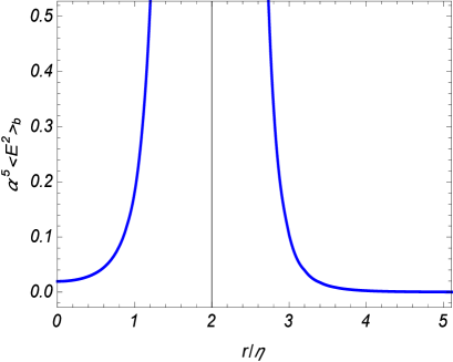
Figure 1: Shell-induced contribution in the VEV of the squared electric field versus the proper distance from the shell axis for the $D=4$ model. For the corresponding value of the shell radius we have taken $a/\eta=2$.

4 VEV of the energy-momentum tensor

Another important local characteristic of the vacuum state is the VEV of the energy-momentum tensor. This VEV is evaluated by using the mode-sum formula

$$\langle T_{\mu}^{\nu}\rangle=\frac{1}{16\pi}\delta_{\mu}^{\nu}g^{\rho l}g^{\sigma m}\sum_{\beta}F_{(\beta)\rho\sigma}F_{(\beta)lm}^{\ast}-\frac{1}{4\pi}g^{\nu\kappa}g^{\rho\sigma}\sum_{\beta}F_{(\beta)\mu\rho}F_{(\beta)\kappa\sigma}^{\ast},$$ (4.1)

where $F_{(\beta)\mu\rho}=\partial_{\mu}A_{(\beta)\rho}-\partial_{\rho}A_{(\beta)\mu}$ is the field strength corresponding to the mode functions (2.5) and (2.6). By using the expressions for the mode functions, the mode-sums for the diagonal components of the VEV are presented in the form (no summation over $i$)

$$\langle T_{i}^{i}\rangle = \frac{2B_{D}\eta^{D+2}}{\alpha^{D+1}a^{2}}\sideset{}{{}^{\prime}}{\sum}_{m=0}^{\infty}\int_{0}^{\infty}dkk^{D-3}\sum\limits_{\lambda=0,1}\sum_{n=1}^{\infty}\gamma_{m,n}^{(\lambda)}$$ (4.2)

$$\times T_{m}(\gamma_{m,n}^{(\lambda)})\sum_{l=0,1}t_{\lambda l}^{(i)}[k,\gamma_{m,n}^{(\lambda)}/a,J_{m}(\gamma r)]L_{D/2-1-l}(\omega_{m,n}^{(\lambda)}\eta),$$

where

$$B_{D}=\frac{2^{2-D}}{\pi^{D/2+1}\Gamma(D/2-1)}.$$ (4.3)

Here we have used the notations

$$t_{\lambda l}^{(i)}[k,\gamma,f(y)]=(a_{\lambda l}^{(i)}k^{2}+b_{\lambda l}^{(i)}\gamma^{2})Z_{m}^{(i)}[f(y)]+(\left(D-3\right)c_{\lambda l}^{(i)}k^{2}+d_{\lambda l}^{(i)}\gamma^{2})f^{2}(y),$$ (4.4)

and

$$Z_{m}^{(i)}[f(y)] = f^{\prime 2}(y)+m^{2}f^{2}(y)/y^{2},\;i=0,3,\ldots,D,$$

$$Z_{m}^{(i)}[f(y)] = f^{\prime 2}(y)-m^{2}f^{2}(y)/y^{2},\;i=1,2.$$ (4.5)

For the energy density the coefficients in (4.4) are given by the expressions

$$a_{\lambda l}^{(0)} = \left(\begin{array}[]{cc}1&1\\ 1&1\end{array}\right),\;b_{\lambda l}^{(0)}=\left(\begin{array}[]{cc}D-2&0\\ 0&1\end{array}\right),$$ (4.10)

$$c_{\lambda l}^{(0)} = \left(\begin{array}[]{cc}1&1\\ 0&0\end{array}\right),\;d_{\lambda l}^{(0)}=\left(\begin{array}[]{cc}0&D-2\\ 1&0\end{array}\right),$$ (4.15)

where the rows and columns are numbered by $\lambda=0,1$ and $l=0,1$, respectively. For the coefficients in the radial and azimuthal components one has

$$a_{\lambda l}^{(1)}=\left(\begin{array}[]{cc}-1&1\\ 1&-1\end{array}\right),\;c_{\lambda l}^{(1)}=\left(\begin{array}[]{cc}1&-1\\ 0&0\end{array}\right),$$ (4.16)

and $a_{\lambda l}^{(2)}=-a_{\lambda l}^{(1)}$, $b_{\lambda l}^{(2)}=-b_{\lambda l}^{(1)}=b_{\lambda l}^{(0)}$, $c_{\lambda l}^{(2)}=c_{\lambda l}^{(1)}$, $d_{\lambda l}^{(1)}=d_{\lambda l}^{(2)}=-d_{\lambda l}^{(0)}$. For the axial components, $i=3,\ldots,D$, we get

$$a_{\lambda l}^{(i)} = \frac{1}{D-2}\left(\begin{array}[]{cc}D-4&2-D\\ D-4&2-D\end{array}\right),\;b_{\lambda l}^{(i)}=\left(\begin{array}[]{cc}D-4&0\\ 0&-1\end{array}\right),$$ (4.21)

$$c_{\lambda l}^{(i)} = \frac{1}{D-2}\left(\begin{array}[]{cc}D-6&4-D\\ 0&0\end{array}\right),\;d_{\lambda l}^{(i)}=\left(\begin{array}[]{cc}0&4-D\\ 1&0\end{array}\right).$$ (4.26)

In addition to the diagonal component, the VEV of the energy-momentum tensor has a nonzero off-diagonal component

$$\langle T_{0}^{1}\rangle = \frac{2^{3-D}i\eta^{D+2}}{\pi^{D}\alpha^{D+1}a^{3}}\sideset{}{{}^{\prime}}{\sum}_{m=0}^{\infty}\int d\mathbf{k}\sum_{n=1}^{\infty}\sum_{\lambda=0,1}(-1)^{\lambda}N_{\lambda}T_{m}(\gamma_{m,n}^{(\lambda)})\omega_{m,n}^{(\lambda)}\gamma_{m,n}^{(\lambda)2}$$ (4.27)

$$\times K_{D/2-2}(\omega_{m,n}^{(\lambda)}\eta e^{-\frac{i\pi}{2}})K_{D/2-1}(\omega_{m,n}^{(\lambda)}\eta e^{\frac{i\pi}{2}})J_{m}(\gamma_{m,n}^{(\lambda)}r/a)J_{m}^{\prime}(\gamma_{m,n}^{(\lambda)}r/a).$$

where $N_{0}=D-2$, $N_{1}=1$. This component describes energy flux along the radial direction (along the direction normal to the boundary).

After the application of the summation formula (3.6), with the function

$$f(x)=xL_{D/2-1-l}(\eta\sqrt{x^{2}/a^{2}+k^{2}})t_{\lambda l}^{(i)}[k,x/a,J_{m}(xr/a)],$$ (4.28)

to the series over $n$ in (4.2), the VEV of the energy-momentum tensor is presented in the form

$$\langle T_{\mu}^{\nu}\rangle=\langle T_{\mu}^{\nu}\rangle_{\mathrm{dS}}+\langle T_{\mu}^{\nu}\rangle_{\mathrm{b}},$$ (4.29)

where $\langle T_{\mu}^{\nu}\rangle_{\mathrm{dS}}$ is the corresponding VEV in the boundary-free dS spacetime and the contribution $\langle T_{\mu}^{\nu}\rangle_{b}$ is induced by the presence of the cylindrical shell. The boundary-free contribution corresponds to the first integral in the right-hand side of the formula (3.6) and the boundary-induced contribution comes from the second integral. For points outside the cylindrical shell the boundary-induced contribution in (4.29) is finite and the renormalization is reduced to the one for the boundary-free part. From the maximal symmetry of the Bunch-Davies vacuum state it follows that the latter does not depend on the spacetime point and has the form $\langle T_{\mu}^{\nu}\rangle_{\mathrm{dS}}=\mathrm{const}\cdot\delta_{\mu}^{\nu}$.

With the help of the transformations similar to those we have used for the VEV of the field squared, for the boundary-induced parts in the diagonal components we get (no summation over $i$)

$$\langle T_{i}^{i}\rangle_{\mathrm{b}} = \frac{B_{D}}{\alpha^{D+1}}\sideset{}{{}^{\prime}}{\sum}_{m=0}^{\infty}\sum\limits_{\lambda=0,1}\int_{0}^{\infty}dx\,x^{D+1}\dfrac{K_{m}^{\left(\lambda\right)}\left(ax/\eta\right)}{I_{m}^{\left(\lambda\right)}\left(ax/\eta\right)}\int_{0}^{1}ds\,s$$ (4.30)

$$\times\left(1-s^{2}\right)^{D/2-2}\sum_{l=0,1}P_{\lambda l}^{(i)}[s,I_{m}(xr/\eta)]f_{D/2-1-l}(xs),$$

where we have defined the functions

$$P_{\lambda l}^{(i)}[s,f(y)]=(A_{\lambda l}^{(i)}+B_{\lambda l}^{(i)}s^{2})Z_{m}^{(i)}[f(y)]+(C_{\lambda l}^{(i)}+\left(D-3\right)D_{\lambda l}^{(i)}s^{2})f^{2}(y),$$ (4.31)

with $Z_{m}^{(i)}[f(y)]$ given by (4.5). For the energy density the coefficients in (4.31) are given by the expressions

$$A_{\lambda l}^{(0)}=C_{\lambda l}^{(0)}=\left(\begin{array}[]{cc}3-D&1\\ 1&0\end{array}\right),\;B_{\lambda l}^{(0)}=-\left(\begin{array}[]{cc}1&1\\ 1&1\end{array}\right),\;D_{\lambda l}^{(0)}=\left(\begin{array}[]{cc}1&1\\ 0&0\end{array}\right).\;$$ (4.32)

For the radial and azimuthal stresses one has

$$A_{\lambda l}^{(i)} = \left(-1\right)^{i}C_{\lambda l}^{(i)}=-\left(-1\right)^{i}\left(\begin{array}[]{cc}D-3&1\\ 1&0\end{array}\right),$$ (4.35)

$$B_{\lambda l}^{(i)} = \left(-1\right)^{i}\left(\begin{array}[]{cc}-1&1\\ 1&-1\end{array}\right),\;D_{\lambda l}^{(i)}=\left(\begin{array}[]{cc}1&-1\\ 0&0\end{array}\right),\;$$ (4.40)

with $i=1,2$. And finally, for the axial stresses ($i=3,\ldots,D$) we get:

$$A_{\lambda l}^{(i)} = \frac{1}{D-2}\left(\begin{array}[]{cc}(D-4)\left(3-D\right)&2-D\\ D-4&0\end{array}\right),\;B_{\lambda l}^{(i)}=\frac{1}{D-2}\left(\begin{array}[]{cc}4-D&D-2\\ 4-D&D-2\end{array}\right),$$ (4.45)

$$C_{\lambda l}^{(i)} = \frac{1}{D-2}\left(\begin{array}[]{cc}\left(3-D\right)\left(D-6\right)&4-D\\ D-2&0\end{array}\right),\;D_{\lambda l}^{(i)}=\frac{1}{D-2}\left(\begin{array}[]{cc}D-6&4-D\\ 0&0\end{array}\right).\;$$ (4.50)

Note that, unlike to the case of the Minkowski bulk (see below), for the dS bulk the axial stresses do not coincide with the energy density.

For the off-diagonal component (4.27), the contribution of the first integral in (3.6) to the VEV vanishes. This directly follows from the relations $\sum_{m=0}^{\prime\infty}J_{m}(x)J_{m}^{\prime}(x)=(1/2)\partial_{x}\sum_{m=0}^{\prime\infty}J_{m}^{2}(x)$ and $\sum_{m=0}^{\prime\infty}J_{m}^{2}(x)=1/2$. The nonzero part is induced by the presence of the shell and is given by the expression

$$\langle T_{0}^{1}\rangle_{\mathrm{b}} = -\frac{2B_{D}}{\alpha^{D+1}}\sideset{}{{}^{\prime}}{\sum}_{m=0}^{\infty}\int_{0}^{\infty}dx\,x^{D+1}\left[(D-2)\frac{K_{m}(xa/\eta)}{I_{m}(xa/\eta)}-\frac{K_{m}^{\prime}(xa/\eta)}{I_{m}^{\prime}(xa/\eta)}\right]I_{m}(xr/\eta)I_{m}^{\prime}(xr/\eta)$$ (4.51)

$$\times\int_{0}^{1}ds\,s^{2}\left(1-s^{2}\right)^{D/2-2}\left[K_{D/2-1}\left(y\right)I_{2-D/2}\left(y\right)-K_{D/2-2}\left(y\right)I_{D/2-1}\left(y\right)\right]_{y=xs}.$$

In the special case $D=3$ the off-diagonal component vanishes. For other values of $D$, for which the representation (4.51) is valid both the functions in the square brackets are positive and, hence, $\langle T_{0}^{1}\rangle_{\mathrm{b}}<0$ for $0<r<a$. On the axis, the energy flux vanishes, $\langle T_{0}^{1}\rangle_{\mathrm{b},r=0}=0$. Similar to the case of the field squared, the boundary-induced VEVs (4.30) and (4.51) depend on $\eta$, $a$, $r$ in the form of the ratios $a/\eta$ and $r/\eta$.

With the expressions (4.30) and (4.51), we can see that the boundary-induced contributions obey the covariant continuity equation $\nabla_{\nu}\langle T_{\mu}^{\nu}\rangle_{b}=0$. For the geometry at hand, this equation is reduced to the following relations between the VEVs:

$$\left(\partial_{\eta}-\frac{D+1}{\eta}\right)\langle T_{0}^{0}\rangle_{\mathrm{b}} = \left(\partial_{r}+\frac{1}{r}\right)\langle T_{0}^{1}\rangle_{\mathrm{b}}-\frac{1}{\eta}\langle T_{k}^{k}\rangle_{\mathrm{b}},$$

$$\left(\partial_{\eta}-\frac{D+1}{\eta}\right)\langle T_{0}^{1}\rangle_{\mathrm{b}} = \frac{1}{r}\langle T_{2}^{2}\rangle_{\mathrm{b}}-\left(\partial_{r}+\frac{1}{r}\right)\langle T_{1}^{1}\rangle_{\mathrm{b}}.$$ (4.52)

Let us denote by $\mathcal{E}_{\mathrm{b},r\leqslant r_{0}}$ the shell-induced contribution in the vacuum energy in the region $r\leqslant r_{0}<a$, per unit coordinate lengths along the directions $z^{3},\ldots,z^{D}$:

$$\mathcal{E}_{\mathrm{b},r\leqslant r_{0}}=2\pi\left(\alpha/\eta\right)^{D}\int_{0}^{r_{0}}dr\,r\langle T_{0}^{0}\rangle_{\mathrm{b}}.$$ (4.53)

By taking into account the first equation in (4.52), the corresponding derivative with respect to the synchronous time coordinate $t$ is expressed as (see also [11])

$$\partial_{t}\mathcal{E}_{\mathrm{b},r\leqslant r_{0}}=\frac{2\pi}{\alpha}\left(\alpha/\eta\right)^{D}\int_{0}^{r_{0}}dr\,r\sum_{l=1}^{D}\langle T_{l}^{l}\rangle_{\mathrm{b}}-2\pi r_{0}\left(\alpha/\eta\right)^{D-1}\langle T_{0}^{1}\rangle_{\mathrm{b},r=r_{0}}.$$ (4.54)

This relation shows that $\langle T_{0}^{1}\rangle_{b}$ is the energy flux per unit proper surface area. The quantity $-\langle T_{l}^{l}\rangle_{b}$ is the shell-induced contribution to the vacuum pressure along the $l$-th direction and the first term in the right-hand side of (4.54) is the work done by the surrounding on the selected volume. The last term in (4.54) is the energy flux through the surface $r=r_{0}$. Inside the shell one has $\langle T_{0}^{1}\rangle_{\mathrm{b}}<0$ and the flux is directed from the shell to the axis $r=0$.

Let us discuss special cases of the general expressions for the VEVs of the energy-momentum tensor components. First we consider the Minkowskian limit, corresponding to $\alpha\rightarrow\infty$. Introducing in (4.30) a new integration variable $y=x/\eta$, we see that the argument of the functions $f_{\nu}(u)$ is large and we can use the asymptotic expression $f_{\nu}(u)\approx 1/u$. After the integration over $s$, to the leading order we get $\langle T_{i}^{i}\rangle_{b}\approx\langle T_{i}^{i}\rangle_{b}^{(\mathrm{M})}$, where for the VEVs on the Minkowski bulk one has (no summation over $i$)

$$\langle T_{i}^{i}\rangle_{\mathrm{b}}^{(\mathrm{M})}=\frac{2(4\pi)^{-(D+1)/2}}{\Gamma((D+1)/2)}\sideset{}{{}^{\prime}}{\sum}_{m=0}^{\infty}\sum\limits_{\lambda=0,1}\int_{0}^{\infty}dxx^{D}\dfrac{K_{m}^{\left(\lambda\right)}\left(ax\right)}{I_{m}^{\left(\lambda\right)}\left(ax\right)}\left\{A_{\lambda}^{(i)}Z_{m}^{(i)}[I_{m}(rx)]+B_{\lambda}^{(i)}I_{m}^{2}(rx)\right\},$$ (4.55)

with the coefficients

$$A_{0}^{(0)} = \left(2-D\right)(D-3),\;A_{1}^{(0)}=D-3,$$

$$B_{0}^{(0)} = (2-D)\left(D-5\right),\;B_{1}^{(0)}=D-1,$$

$$A_{\lambda}^{(l)} = \left(-1\right)^{l}B_{\lambda}^{(l)},\;B_{0}^{(l)}=(2-D)\left(D-1\right),\;B_{1}^{(l)}=1-D,$$ (4.56)

for $l=1,2$. For the stresses along the directions $i=3,\ldots,D$ we have $\langle T_{i}^{i}\rangle_{b}^{(\mathrm{M})}=\langle T_{0}^{0}\rangle_{b}^{(\mathrm{M})}$. In the special case $D=3$, from (4.55) we obtain the results previously derived in [21]. As is seen, for the Minkowski bulk the axial stresses are equal to the energy density. This result could be directly obtained on the base of the invariance of the problem with respect to the Lorentz boosts along the directions of the axis $x^{i}$, $i=3,\ldots,D$. The off-diagonal component vanishes in the Minkowskian limit. For the leading term in the corresponding asymptotic expansion from (4.51) we find

$$\langle T_{0}^{1}\rangle_{\mathrm{b}}\approx\frac{3-D}{\alpha}\frac{2^{1-D}\pi^{-(D+1)/2}}{\Gamma((D-1)/2)}\sideset{}{{}^{\prime}}{\sum}_{m=0}^{\infty}\int_{0}^{\infty}dx\,x^{D-1}\left[(D-2)\frac{K_{m}(ax)}{I_{m}(ax)}-\frac{K_{m}^{\prime}(ax)}{I_{m}^{\prime}(ax)}\right]I_{m}(xr)I_{m}^{\prime}(xr).$$ (4.57)

In the special case $D=3$ the off-diagonal component of the vacuum energy-momentum tensor vanishes, $\langle T_{0}^{1}\rangle_{\mathrm{b}}=0$, and the diagonal components are connected to the corresponding quantities for a cylindrical shell in the Minkowski bulk by the relation (no summation over $i$)

$$\langle T_{i}^{i}\rangle_{\mathrm{b}}=(\eta/\alpha)^{4}\langle T_{i}^{i}\rangle_{\mathrm{b}}^{(\mathrm{M})}.$$ (4.58)

In this special case $A_{\lambda}^{(i)}=0$ for $i=0,3$, and $B_{0}^{(i)}=B_{1}^{(i)}$ for all $i$. Note that the Casimir self-stress for an infinite perfectly conducting cylindrical shell in background of 4-dimensional Minkowski spacetime has been evaluated in [22] on the base of a Green’s function technique. The corresponding Casimir energy was investigated by using the zeta function technique in [23] and the mode-by-mode summation method in [24]. The geometry of a cylindrical shell coaxial with a cosmic string was considered in [17, 25].

Near the cylindrical shell, the asymptotic expressions for the components of the energy-momentum tensor are found in the way similar to that for the VEV of the electric field squared, by using the uniform asymptotic expansions for the modified Bessel functions. The leading terms are given by the expressions (no summation over $i$)

$$\langle T_{i}^{i}\rangle_{\mathrm{b}}\approx-\frac{\left(D-1\right)(D-3)\Gamma((D+1)/2)}{2(4\pi)^{(D+1)/2}[\alpha\left(a-r\right)/\eta]^{D+1}},$$ (4.59)

for $i=0,2,\ldots,D$, and

$$\langle T_{0}^{1}\rangle_{\mathrm{b}}\approx\frac{a-r}{\eta}\langle T_{0}^{0}\rangle_{b},\;\langle T_{1}^{1}\rangle_{\mathrm{b}}\approx\frac{a-r}{Da}\langle T_{0}^{0}\rangle_{b}.$$ (4.60)

The leading terms for the diagonal components coincide with those for a cylindrical shell in Minkowski bulk with the distance from the shell replaced by the proper distance $\alpha\left(a-r\right)/\eta$. In the special case $D=3$ the leading terms vanish. The latter feature is related to the conformal invariance of the electromagnetic field in $D=3$.

In the special case $D=4$, the integrals over $s$ in (4.30) are evaluated in appendix B. The expression for the diagonal components takes the form (no summation over $i$)

$$\langle T_{i}^{i}\rangle_{\mathrm{b}} = \frac{\alpha^{-5}}{4\pi^{3}}\sideset{}{{}^{\prime}}{\sum}_{m=0}^{\infty}\sum\limits_{\lambda=0,1}\int_{0}^{\infty}dxx^{5}\dfrac{K_{m}^{\left(\lambda\right)}\left(ax/\eta\right)}{I_{m}^{\left(\lambda\right)}\left(ax/\eta\right)}$$ (4.61)

$$\times\sum_{l=0,1}\left\{(A_{\lambda l}^{(i)}\mathcal{I}_{1,1-l}(x)+B_{\lambda l}^{(i)}\mathcal{I}_{3,1-l}(x))Z_{m}^{(i)}[I_{m}(xr/\eta)]\right.$$

$$\left.+(C_{\lambda l}^{(i)}\mathcal{I}_{1,1-l}(x)+D_{\lambda l}^{(i)}\mathcal{I}_{3,1-l}(x))I_{m}^{2}(xr/\eta)\right\},$$

where the coefficients are given by (4.32), (4.40) and (4.50) with $D=4$. In the expression (4.51) for the energy flux, with $D=4$, the integral over $s$ is evaluated by using the formulas (B.3) and (B.4). This leads to the following result:

$$\langle T_{0}^{1}\rangle_{\mathrm{b}} = -\frac{\alpha^{-5}}{2\pi^{3}}\sideset{}{{}^{\prime}}{\sum}_{m=0}^{\infty}\int_{0}^{\infty}dx\,x^{4}\left[2\frac{K_{m}(ax/\eta)}{I_{m}(ax/\eta)}-\frac{K_{m}^{\prime}(ax/\eta)}{I_{m}^{\prime}(ax/\eta)}\right]$$ (4.62)

$$\times I_{m}(xr/\eta)I_{m}^{\prime}(xr/\eta)I_{1}\left(x\right)K_{1}\left(x\right).$$

In figure 2 we have plotted the boundary-induced contribution in the energy density and the energy flux as functions of the proper distance from the shell axis, measured in units of the dS curvature scale $\alpha$. For the corresponding value of the shell radius we have taken $a/\eta=2$. As is seen, in the interior region the energy density is negative near the shell and positive near the axis of the shell. The energy flux is negative inside the shell. This means that the energy flux is directed from the shell. The corresponding energy density in the Minkowski bulk is negative everywhere.

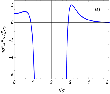
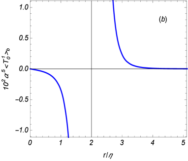
Figure 2: Shell-induced contribution in the VEV of the energy density (panel (a)) and the energy flux (panel (b)) as functions of the ratio $r/\eta$ in the $D=4$ model. The graphs are plotted for $a/\eta=2$.

5 Exterior region

In the region outside the shell, $r>a$, the radial functions $C_{m}(x)$ in (2.5) and (2.6) are linear combinations of the Bessel and Neumann functions. The relative coefficients in the linear combinations are determined from the boundary condition (2.3) on the cylindrical surface $r=a$. In this way we can see that

$$C_{m}(\gamma r)=g_{m}^{(\lambda)}(\gamma a,\gamma r)=J_{m}(\gamma r)Y_{m}^{(\lambda)}(\gamma a)-Y_{m}(\gamma r)J_{m}^{(\lambda)}(\gamma a),$$ (5.1)

for the modes $\lambda=0,1$. Now, in the normalization condition (2.11) the integration over the radial coordinate goes over the region $a\leqslant r<\infty$ and in the right-hand side the delta symbol for the quantum number $\gamma$ is understood as the Dirac delta function $\delta(\gamma-\gamma^{\prime})$. As the normalization integral diverges for $\gamma^{\prime}=\gamma$, the main contribution to the integral comes from large values of $r$. By making use of the asymptotic formulas for the Bessel and Neumann functions with large arguments, for the normalization coefficients in (2.5) and (2.6) one gets

$$\left|c_{\beta}\right|^{2}=\frac{[J_{m}^{(\lambda)2}(\gamma a)+Y_{m}^{(\lambda)2}(\gamma a)]^{-1}}{4\left(2\pi\alpha\right)^{D-3}\gamma}.$$ (5.2)

Similar to the case of the interior region, we consider the VEVs of the field squared and energy-momentum tensor separately.

5.1 VEV of the field squared

For the VEV of the electric field squared, by using the mode-sum formula (3.1), one finds

$$\langle E^{2}\rangle = \frac{2^{5}A_{D}\eta^{D+2}}{\alpha^{D+1}}\ \sideset{}{{}^{\prime}}{\sum}_{m=0}^{\infty}\int_{0}^{\infty}dkk^{D-3}\int_{0}^{\infty}d\gamma\,$$ (5.3)

$$\times\gamma^{3}\sum\limits_{\lambda=0,1}\frac{G_{m}^{(\lambda)}[k,g_{m}^{(\lambda)}(\gamma a,\gamma r)]}{J_{m}^{(\lambda)2}(\gamma a)+Y_{m}^{(\lambda)2}(\gamma a)}L_{D/2-2}(\omega\eta),$$

with the same notations as in (3.2). With the help of the identity

$$\frac{G_{m}^{(\lambda)}[k,g_{m}^{(\lambda)}(\gamma a,\gamma r)]}{J_{m}^{(\lambda)2}(\gamma a)+Y_{m}^{(\lambda)2}(\gamma a)}=G_{m}^{(\lambda)}[J_{m}(\gamma r)]-\frac{1}{2}\sum\limits_{j=0,1}\frac{J_{m}^{\left(\lambda\right)}\left(\gamma a\right)}{H_{m}^{\left(j\right)\left(\lambda\right)}\left(\gamma a\right)}G_{m}^{(\lambda)}[k,H_{m}^{\left(j\right)}(\gamma r)],$$ (5.4)

the VEV is presented in the decomposed form (3.11) where the shell-induced contribution is given by the expression

$$\langle E^{2}\rangle_{\mathrm{b}} = -\frac{2^{4}A_{D}\eta^{D+2}}{\alpha^{D+1}}\sideset{}{{}^{\prime}}{\sum}_{m=0}^{\infty}\int_{0}^{\infty}dkk^{D-3}\ \sum\limits_{j=0,1}$$ (5.5)

$$\times\sum\limits_{\lambda=0,1}\int_{0}^{\infty}d\gamma\gamma^{3}\frac{J_{m}^{\left(\lambda\right)}\left(\gamma a\right)}{H_{m}^{\left(j\right)\left(\lambda\right)}\left(\gamma a\right)}L_{D/2-2}(\omega\eta).$$

For the further transformation, in (5.5), we rotate the contour of integration in the complex plane $\gamma$ by the angle $\pi/2$ for the term with $j=1$ and by the angle $-\pi/2$ for $j=2$. Introducing the modified Bessel functions, the expression (5.5) takes the form

$$\langle E^{2}\rangle_{\mathrm{b}} = \frac{2^{5}A_{D}}{\alpha^{D+1}}\sideset{}{{}^{\prime}}{\sum}_{m=0}^{\infty}\sum\limits_{\lambda=0,1}\int_{0}^{\infty}dx\,x^{D+1}\dfrac{I_{m}^{\left(\lambda\right)}\left(ax/\eta\right)}{K_{m}^{\left(\lambda\right)}\left(ax/\eta\right)}$$ (5.6)

$$\times\int_{0}^{1}dss\left(1-s^{2}\right)^{D/2-2}G_{m}^{\left(\lambda\right)}\left[s,K_{m}\left(xr/\eta\right)\right]f_{D/2-2}\left(xs\right),$$

where the functions $G_{m}^{(\lambda)}\left[s,f(x)\right]$ are defined by the formulae (3.15). Comparing this result with (3.14), we see that the expressions for the interior and exterior regions are related by the interchange $I_{m}\rightleftarrows K_{m}$. In particular, the result in the Minkowskian limit is obtained from (3.16) by the same replacements. In the special case $D=3$ the electromagnetic field is conformally invariant and we have the relation (3.18). Similar to the case of the interior region, the shell-induced contribution (5.5) in the VEV of the electric field squared is positive. For points near the shell, the leading term in the asymptotic expansion over the distance from the boundary is obtained from (3.20) by the replacement $a-r\rightarrow r-a$.

At large proper distances from the shell compared with the dS curvature radius, we have $r/\eta\gg 1$. Introducing in (5.5) a new integration variable $y=xr/\eta$ and assuming that $r\gg a$, we use the expansions of the functions $I_{m}^{\left(\lambda\right)}\left(ya/r\right)/K_{m}^{\left(\lambda\right)}\left(ya/r\right)$ and $f_{D/2-2}\left(ys\eta/r\right)$ for small values of the arguments. The leading contribution comes from the term with $\lambda=0$ and $m=0$. For even $D>4$ one gets

$$\langle E^{2}\rangle_{\mathrm{b}}\approx\frac{4\left(4D^{2}-3D-4\right)\Gamma^{3}(D/2+1)}{\pi^{D/2}D(D-4)\Gamma(D+2)(\alpha r/\eta)^{D+2}}\frac{\alpha}{\ln(r/a)}.$$ (5.7)

In the case $D=4$ the leading term is given by

$$\langle E^{2}\rangle_{\mathrm{b}}\approx\frac{16\pi^{-2}\alpha(\alpha r/\eta)^{-6}}{5\ln(r/a)\ln(r/\eta)}.$$ (5.8)

For $D=3$ and $D=5$ we find

$$\langle E^{2}\rangle_{\mathrm{b}} \approx \frac{2(\alpha r/\eta)^{-4}}{3\pi\ln(r/a)},\;D=3,$$

$$\langle E^{2}\rangle_{\mathrm{b}} \approx \frac{7(\alpha r/\eta)^{-6}}{10\pi^{2}\ln(r/a)},\;D=5.$$ (5.9)

At large distances, the total VEV is dominated by the boundary-free part $\langle E^{2}\rangle_{\mathrm{dS}}$. For a cylindrical shell in the Minkowski bulk, at large distances, $r\gg a$, one has the following asymptotic behavior:

$$\left\langle E^{2}\right\rangle_{\mathrm{b}}^{(\mathrm{M})}\approx\frac{\left(D-2\right)\left(3D-1\right)}{\pi^{(D-1)/2}r^{D+1}\ln(r/a)}\frac{\Gamma^{3}((D+1)/2)}{\left(D-1\right)\Gamma(D+1)},$$ (5.10)

for all values $D\geqslant 3$. Note that for $D=3,5$ the leading term (5.10) is obtained from (5.9) by the replacement of the proper distance from the axis, $\alpha r/\eta\rightarrow r$.

For the special case $D=4$, the shell-induced contribution in the VEV of the squared electric field, for the exterior region, is presented in figure 1 as a function of the ratio $r/\eta$. Similar to the region inside the shell, the corresponding Casimir-Polder force is directed toward the shell.

5.2 Energy-momentum tensor

Now let us consider the VEV of the energy-momentum tensor outside the cylindrical shell. By using the mode-sum formula (4.1) with the exterior modes, for the VEV of the diagonal components we get the following representation (no summation over $i$)

$$\langle T_{i}^{i}\rangle = \frac{B_{D}\eta^{D+2}}{\alpha^{D+1}}\sideset{}{{}^{\prime}}{\sum}_{m=0}^{\infty}\int_{0}^{\infty}dkk^{D-3}\sum\limits_{\lambda=0,1}\int_{0}^{\infty}d\gamma\gamma$$ (5.11)

$$\times\sum_{l=1,2}\frac{t_{\lambda l}^{(i)}[k,\gamma,g_{m}^{(\lambda)}(\gamma a,\gamma r)]}{J_{m}^{(\lambda)2}(\gamma a)+Y_{m}^{(\lambda)2}(\gamma a)}L_{D/2-1-l}(\omega\eta),$$

with the notation (4.4). The expression for the off-diagonal component has the form

$$\langle T_{0}^{1}\rangle = \frac{2iB_{D}\eta^{D+2}}{\alpha^{D+1}}\sideset{}{{}^{\prime}}{\sum}_{m=0}^{\infty}\int_{0}^{\infty}dkk^{D-3}\int_{0}^{\infty}d\gamma\gamma\sum_{\lambda=0,1}(-1)^{\lambda}N_{\lambda}\omega\gamma^{2}$$ (5.12)

$$\times K_{D/2-2}(\omega\eta e^{-\frac{i\pi}{2}})K_{D/2-1}(\omega\eta e^{\frac{i\pi}{2}})\frac{g_{m}^{(\lambda)}(\gamma a,\gamma r)g_{m}^{(\lambda)\prime}(\gamma a,\gamma r)}{J_{m}^{(\lambda)2}(\gamma a)+Y_{m}^{(\lambda)2}(\gamma a)},$$

where $g_{m}^{(\lambda)\prime}(x,y)=\partial_{y}g_{m}^{(\lambda)}(x,y)$.

Further transformation of the VEVs is similar to that we have used for the field squared. In the case of the diagonal components we employ the relation

$$\frac{t_{\lambda l}^{(i)}[k,\gamma,g_{m}^{(\lambda)}(\gamma a,\gamma r)]}{J_{m}^{(\lambda)2}(\gamma a)+Y_{m}^{(\lambda)2}(\gamma a)}=t_{\lambda l}^{(i)}[k,\gamma,J_{m}(\gamma r)]-\frac{1}{2}\sum\limits_{j=1,2}\frac{J_{m}^{\left(\lambda\right)}\left(\gamma a\right)}{H_{m}^{\left(j\right)\left(\lambda\right)}\left(\gamma a\right)}t_{\lambda l}^{(i)}[k,\gamma,H_{m}^{\left(j\right)}(\gamma r)],$$ (5.13)

The part with the first term in the right-hand side coincides with the VEV in the boundary-free dS spacetime. In the part corresponding to the last term in (5.13) we rotate the integration contours by the angle $\pi/2$ for the term with $j=1$ and by the angle $-\pi/2$ for $j=2$. In this way for the boundary-induced contributions in the VEVs of the diagonal components we find (no summation over $i$)

$$\langle T_{i}^{i}\rangle_{\mathrm{b}} = \frac{B_{D}}{\alpha^{D+1}}\sideset{}{{}^{\prime}}{\sum}_{m=0}^{\infty}\sum\limits_{\lambda=0,1}\int_{0}^{\infty}dxx^{D+1}\dfrac{I_{m}^{\left(\lambda\right)}\left(ax/\eta\right)}{K_{m}^{\left(\lambda\right)}\left(ax/\eta\right)}\int_{0}^{1}ds\,s$$ (5.14)

$$\times\left(1-s^{2}\right)^{D/2-2}\sum_{l=0,1}P_{\lambda l}^{(i)}[s,K_{m}(xr/\eta)]f_{D/2-1-l}(xs).$$

In a similar way, the expression for the VEV of the off-diagonal component is presented as

$$\langle T_{0}^{1}\rangle_{\mathrm{b}} = -\frac{2B_{D}}{\alpha^{D+1}}\sideset{}{{}^{\prime}}{\sum}_{m=0}^{\infty}\int_{0}^{\infty}dx\,x^{D+1}\left[(D-2)\frac{I_{m}(xa/\eta)}{K_{m}(xa/\eta)}-\frac{I_{m}^{\prime}(xa/\eta)}{K_{m}^{\prime}(xa/\eta)}\right]K_{m}(xr/\eta)K_{m}^{\prime}(xr/\eta)$$ (5.15)

$$\times\int_{0}^{1}ds\,s^{2}\left(1-s^{2}\right)^{D/2-2}\left[K_{D/2-1}\left(y\right)I_{2-D/2}\left(y\right)-K_{D/2-2}\left(y\right)I_{D/2-1}\left(y\right)\right]_{y=xs}.$$

For $D\geqslant 4$, in the range of validity of this representation one has $\langle T_{0}^{1}\rangle_{\mathrm{b}}>0$. The corresponding energy flux is directed from the cylindrical shell to the infinity. Again, we can see that the shell-induced contributions obey the relations (4.52).

The VEVs in the Minkowskian limit, $\alpha\rightarrow\infty$, are obtained in the way similar to that for the interior region. In this limit the energy flux vanishes and the corresponding expressions for the diagonal components are obtained from (4.55) by the replacements $I_{m}\rightleftarrows K_{m}$. In the special case $D=3$, the VEVs in the dS and Minkowski bulks are connected by the conformal relation (4.58).

For points near the shell, the leading terms in the asymptotic expansions over the distance from the boundary for the components $\langle T_{i}^{i}\rangle_{\mathrm{b}}$ with $i\neq 1$ are given by (4.59) with the replacement $a-r\rightarrow r-a$. For the normal stress and the energy flux we have the relations (4.60). Hence, near the shell and for $D>3$, the boundary-induced contribution in the energy density has the same sign in the exterior and interior regions, whereas the normal stress and the energy flux have opposite signs.

Let us consider the asymptotics of the boundary-induced contributions at large distances from the shell. Introducing in (5.14) and (5.15) a new integration variable $y=xr$, we see that for $r\gg a,\eta$ the arguments of the functions $I_{m}^{\left(\lambda\right)}$, $K_{m}^{\left(\lambda\right)}$ and $f_{D/2-1-l}$ are small. By using the corresponding asymptotic expressions one can show that the dominant contribution comes from the term $m=0$ and $\lambda=0$. For even values of $D>4$, to the leading order one gets the following expressions (no summation over $i$)

$$\langle T_{i}^{i}\rangle_{\mathrm{b}} \approx \frac{2^{D-2}\Gamma^{2}(D/2+1)\Gamma^{2}(D/2)}{(D-2)\left(D-4\right)\Gamma(D+2)}\frac{\alpha B_{D}C_{D}^{(i)}}{(\alpha r/\eta)^{D+2}\ln(r/a)},$$

$$\langle T_{0}^{1}\rangle_{\mathrm{b}} \approx \frac{2^{D-4}D\Gamma^{4}(D/2)B_{D}}{\Gamma(D)(\alpha r/\eta)^{D+1}\ln(r/a)},$$ (5.16)

with the coefficients

$$C_{D}^{(0)} = D(D-1)\left(6-D\right)-6,$$

$$C_{D}^{(1)} = D\left(D-6\right)+2,$$

$$C_{D}^{(2)} = D^{2}\left(3-D\right)-2,$$

$$C_{D}^{(l)} = D^{2}\left(6-D\right)-8D-6,$$ (5.17)

$l=3,\ldots,D$. The corresponding energy density is positive. by taking into account that near the shell the energy density is negative for $D\geqslant 4$, we conclude that at some intermediate value of the radial coordinate the boundary-induced contribution in the energy density vanishes. The asymptotic (5.16) for the energy flux is valid in the case $D=4$ as well. For $D=4$, the leading term in the expansion of the diagonal components is given by (no summation over $i$)

$$\langle T_{i}^{i}\rangle_{\mathrm{b}}\approx\frac{\alpha\ln(r/\eta)C_{4}^{(i)}}{20\pi^{3}(\alpha r/\eta)^{6}\ln(r/a)},$$ (5.18)

where $C_{4}^{(0)}=-C_{4}^{(2)}=3$, and $C_{4}^{(i)}=-1$ for$\;i=1,3,4$. For the Minkowski bulk, the large distance asymptotic is given by (no summation over $i$)

$$\langle T_{i}^{i}\rangle_{\mathrm{b}}^{(\mathrm{M})}\approx\frac{\pi^{-(D+1)/2}\left(2-D\right)\Gamma^{3}((D+1)/2)}{4r^{D+1}\ln(r/a)\left(D-1\right)\Gamma(D+1)}C_{(\mathrm{M})}^{(i)},$$ (5.19)

where

$$C_{(\mathrm{M})}^{(0)} = D^{2}-4D+1,\;i=0,3,\ldots,D,$$

$$C_{(\mathrm{M})}^{(1)} = 1-D,\;C_{(\mathrm{M})}^{(2)}=D(D-1).$$ (5.20)

The corresponding energy density is positive for $D=3$ and negative for $D\geqslant 4$.

The shell-induced contribution to the energy density and the energy flux in the exterior region are plotted in figure 2 for the $D=4$ model. The large distance asymptotic is given by (5.18) and the energy density is positive. For points near the shell we have the asymptotic behavior (4.59), with the replacement $a-r\rightarrow r-a$, and the energy density is negative. Note that for the $D=4$ Minkowski bulk the corresponding energy density is negative everywhere. For the $D=3$ model, the energy density is positive in the exterior region and negative in the interior region.

In the discussion above we have considered the boundary condition (2.3) that generalizes the condition at the surface of a conductor for arbitrary number of spatial dimensions. Another type of boundary conditions for a gauge field is used in bag models of hadrons and in flux tube models of confinement in quantum chromodynamics (see, for instance, [26]). This boundary condition has the form

$$n^{\mu}F_{\mu\nu}=0,$$ (5.21)

on the boundary of a volume inside of which the gluons are confined. In flux tube models the gauge field is confined inside a cylinder. The corresponding Casimir densities inside and outside a cylindrical shell are investigated in a way similar to that we have described above. The mode functions still have the form (2.5) and (2.6). Imposing the boundary condition (5.21), we can see that, in the interior region, eigenvalues for $\gamma$ are roots of the equation (2.10) for the mode $\sigma=1$ and the roots of (2.9) for $\sigma=2,\ldots,D-1$. The final expressions for the VEVs are obtained from those given above by the replacement

$$\dfrac{K_{m}^{\left(\lambda\right)}\left(xa/\eta\right)}{I_{m}^{\left(\lambda\right)}\left(xa/\eta\right)}\rightarrow\dfrac{K_{m}^{\left(1-\lambda\right)}\left(xa/\eta\right)}{I_{m}^{\left(1-\lambda\right)}\left(xa/\eta\right)},$$ (5.22)

in both the interior and exterior regions. In particular, the VEV of the squared electric field is negative in these regions.

6 Conclusion

In the investigations of the Casimir effect the cylindrically symmetric boundaries are among the most popular geometries. In the present paper we have investigated the local Casimir densities for the electromagnetic field inside and outside a cylindrical shell in background of $(D+1)$-dimensional dS spacetime. On the shell, the field tensor obeys the boundary condition (2.3). In the special case $D=3$ this corresponds to the perfect conductor boundary condition. The procedure, we employed for the evaluation of the VEVs bilinear in the field, is based on the mode-sum formula (2.14). In this procedure the complete set of cylindrical mode functions for the electromagnetic field, obeying the boundary condition, is required. In the problem under consideration one has a single mode of the TE type and $D-2$ modes of the TM type. For the Bunch-Davies vacuum state the corresponding vector potentials are given by the expressions (2.5) and (2.6) with the radial functions (2.8) and (5.1) for the exterior and interior regions, respectively.

We have investigated the combined effects of a cylindrical boundary and background gravitational field on the VEVs of the electric field squared and of the energy-momentum tensor. In the interior region the eigenvalues of the quantum number $\gamma$ are expressed in terms of the zeros of the Bessel function $J_{m}(x)$ for the TM modes and in terms of the zeros of the derivative $J_{m}^{\prime}(x)$ in the case of the TE mode. For the summation of the series over these zeros we have used the generalized Abel-Plana summation formula (3.6). This allowed us to extract from the VEVs the parts corresponding to the boundary-free dS spacetime and to present the shell-induced contributions in terms of strongly convergent integrals, for points away from the boundary. With this separation, the renormalization of the VEVs is reduced to the one for the boundary-free geometry. As a result, inside the shell, the VEVs are decomposed as (3.11) and (4.29) with the shell-induced parts given by (3.14) for the electric field squared and by (4.30) for the diagonal components of the energy-momentum tensor. A similar decomposition is provided for the exterior region. The expressions for the shell-induced parts in this region differ from the ones inside the shell by the replacements $I_{m}\rightleftarrows K_{m}$ of the modified Bessel functions (see (5.6) and (5.14)). For both the interior and exterior regions the shell-induced contributions to the VEV of the electric field squared are positive. In addition to the diagonal components, the VEV of the energy-momentum tensor has nonzero off-diagonal component $\langle T_{0}^{1}\rangle$. It corresponds to the energy flux along the radial direction and is given by the expressions (4.51) and (5.15) for the exterior and interior regions. The off-diagonal component is negative inside the shell and positive in the exterior region. This means that the energy flux is directed from the shell in both the regions. On the axis of the shell the flux vanishes.

We have considered various special cases of general formulas. In the limit $\alpha\rightarrow\infty$, the VEVs inside and outside a cylindrical shell in the background of $(D+1)$-dimensional Minkowski spacetime are obtained. The corresponding expressions generalize the results previously known for $D=3$ to an arbitrary number of spatial dimensions. Note that for $D=3$ the electromagnetic field is conformally invariant and the shell-induced VEVs in the dS bulk are obtained from those in Minkowski spacetime by the standard conformal transformation. For points near the cylindrical boundary the contribution of small wavelengths dominates in the shell-induced VEVs. The leading terms in the corresponding asymptotic expansions for the field squared and diagonal components of the energy-momentum tensor coincide with those for a cylindrical shell in the Minkowski bulk with the distance from the shell replaced by the proper distance in dS bulk. The leading term in the energy flux is given by the relation (4.60). The effects of the background gravitational field on the shell-induced VEVs are essential at distances from the boundary larger than the curvature radius of the dS spacetime. In particular, for the numerical example considered by us in the case $D=4$, at large distances the shell-induced contribution to the vacuum energy density is negative for the Minkowski bulk and positive for dS background. Near the shell, the energy density is negative in both these cases. As a consequence, for the dS bulk it vanishes for some intermediate value of the radial coordinate.

Another boundary condition, used for the confinement of gauge fields in bag models of hadrons and in flux tube models of QCD, is the one given by (5.21). The corresponding expressions for the VEVs of the field squared and energy-momentum tensor are obtained from those for generalized perfect conductor boundary condition by the replacement (5.22). In this case, the boundary-induced contribution on the VEV of the squared electric field is neagtive in both the interior and exterior regions.

Appendix A Cylindrical modes in Minkowski spacetime

In this section we consider the cylindrical modes for the electromagnetic field in $(D+1)$-dimensional Minkowski spacetime. For the electromagnetic field one has $D-1$ polarization states specified by $\sigma=1,2,\ldots,D-1$. The vector potential for the polarization $\sigma$ will be denoted by $A_{\sigma\mu}$, $\mu=0,1,\ldots,D$. We will impose the gauge condition $\nabla_{(\mathrm{M})\mu}A_{\sigma}^{\mu}=0$, where $\nabla_{(\mathrm{M})\mu}$ is the covariant derivative operator associated with the Minkowskian metric tensor $g_{(\mathrm{M})\mu\nu}=\mathrm{diag}(1,-1,-r^{2},-1,\ldots,-1)$. From the field equation $\nabla_{(\mathrm{M})\mu}F^{\mu\nu}=0$ one gets

$$\left(\Delta-\partial_{0}^{2}\right)A_{\sigma\mu}=0,$$ (A.1)

for $\mu=0,3,\ldots,D$, and

$$\left(\partial_{0}^{2}-\Delta\right)A_{\sigma 1}+\frac{A_{\sigma 1}}{r^{2}}+\frac{2}{r^{3}}\partial_{2}A_{\sigma 2} = 0,$$

$$\partial_{0}^{2}A_{\sigma 2}-\Delta A_{\sigma 2}+\frac{2}{r}\partial_{1}A_{\sigma 2}-\frac{2}{r}\partial_{2}A_{\sigma 1} = 0,$$ (A.2)

for the radial and azimuthal components. Here

$$\Delta=\frac{1}{r}\partial_{1}\left(r\partial_{1}\right)+\frac{1}{r^{2}}\partial_{2}^{2}+\sum_{l=3}^{D}\partial_{l}^{2}.$$ (A.3)

For the polarization $\sigma=1$ we take

$$A_{\sigma\mu}=(0,-r^{-1}\partial_{2},r\partial_{1},0,\ldots,0)\psi_{\sigma},\;\sigma=1.$$ (A.4)

It can be easily checked that this function obeys the gauge condition. The field equations (A.2) are satisfied if the function $\psi_{\sigma}$ obeys the equation

$$\left(\Delta-\partial_{0}^{2}\right)\psi_{\sigma}=0.$$ (A.5)

For the polarizations $\sigma=2,\ldots,D-1$ we present the vector potential in the form

$$A_{\sigma\mu}=\epsilon_{\sigma\mu}\psi_{\sigma},\;\sigma=2,\ldots,D-1,$$ (A.6)

with scalar functions $\psi_{\sigma}$ and $\epsilon_{\sigma 1}=\epsilon_{\sigma 2}=0$. From the field equations (A.1) it follows that the functions $\psi_{\sigma}$ obey the wave equation (A.5). The gauge condition is reduced to

$$g_{(\mathrm{M})}^{\mu\nu}\epsilon_{\sigma\mu}\partial_{\nu}\psi_{\sigma}=0.$$ (A.7)

The solutions for the scalar functions $\psi_{\sigma}$, $\sigma=1,2,\ldots,D-1$, have the form

$$\psi_{\sigma}=C_{m}(\gamma r)e^{i(m\phi+\mathbf{k}\cdot\mathbf{z}-\omega t)},$$ (A.8)

where $C_{m}(x)$ is a cylinder function of the order $m=0,\pm 1,\pm 2,\ldots$, $\mathbf{k}\cdot\mathbf{z}=\sum_{l=3}^{D}k_{l}z^{l}$, and $\omega$ is given by (2.7). We will normalize the polarization vectors in accordance with the relation

$$g_{(\mathrm{M})}^{\mu\nu}\epsilon_{\sigma\mu}\epsilon_{\sigma^{\prime}\nu}=-\frac{\gamma^{2}}{\omega^{2}}\delta_{\sigma\sigma^{\prime}}.$$ (A.9)

From the gauge condition one has $\epsilon_{\sigma 0}=-\mathbf{k}\cdot\mathbf{\epsilon}_{\sigma}/\omega$, where $\mathbf{k}\cdot\mathbf{\epsilon}_{\sigma}=\sum_{l=3}^{D}k_{l}\epsilon_{\sigma l}$. Combining with (A.9) the following relations are obtained:

$$\sum_{l,n=3}^{D}\left(\omega^{2}\delta_{nl}-k_{l}k_{n}\right)\epsilon_{\sigma l}\epsilon_{\sigma^{\prime}n}=\gamma^{2}\delta_{\sigma\sigma^{\prime}},$$ (A.10)

and

$$\sum_{\sigma=2}^{D-1}\epsilon_{\sigma l}\epsilon_{\sigma n}=\omega^{-2}(k_{l}k_{n}+\gamma^{2}\delta_{ln}),$$ (A.11)

for $l,n=3,\ldots,D$.

An alternative form for the cylindrical modes (A.6) with the polarizations $\sigma=2,\ldots,D-1$ is obtained by making the gauge transformation

$$A_{\sigma\mu}^{\prime}=A_{\sigma\mu}+\partial_{\mu}f_{\sigma},$$ (A.12)

with the function

$$f_{\sigma}=i\omega^{-2}\mathbf{k}\cdot\mathbf{\epsilon}_{\sigma}\psi_{\sigma}.$$ (A.13)

In the new gauge the scalar potential vanishes, $A_{\sigma 0}^{\prime}=0$, and one has

$$A_{\sigma\mu}^{\prime}=\left(0,\left(\epsilon_{\sigma l}+i\omega^{-2}\mathbf{k}\cdot\mathbf{\epsilon}_{\sigma}\partial_{l}\right)\psi_{\sigma}\right),\;l=1,\ldots,D.$$ (A.14)

Hence, for $(D+1)$-dimensional Minkowski spacetime the cylindrical modes for the electromagnetic field in the gauge $A_{\sigma 0}=0$, $\partial_{l}(rA^{l})=0$ are given by (A.4) and (A.14), where for the scalar function $\psi_{\sigma}$ one has the expression (A.8). The radial function $C_{m}(\gamma r)$ is a linear combination of the Bessel and Neumann functions. The relative coefficient in this linear combination depends on the specific problem. For example, inside a cylindrical shell one has $C_{m}(\gamma r)\sim J_{m}(\gamma r)$. In the special case $D=3$, the modes (A.4) and (A.14) are reduced to the well known TE and TM modes in cylindrical waveguides (see, for instance, [27]). In the $(D+1)$-dimensional case we have a single mode of the TE type and $D-2$ modes of the TM type. The corresponding boundary conditions are discussed in section 2.

Appendix B Evaluation of the integrals in the model $D=4$

In this section we evaluate the integrals of the form (3.22) appearing in the expressions for the VEVs in the special case $D=4$. First of all, by using the integration formula from [28] we can see that

$$\mathcal{I}_{1,0}(x) = \frac{1}{2}\left[f_{0}(x)+f_{1}(x)\right],$$

$$\mathcal{I}_{1,1}(x) = \mathcal{I}_{1,0}(x)-\frac{2}{x}I_{1}(x)K_{0}(x).$$ (B.1)

Our starting point in the evaluation of the remaining integrals is the formula (see, for instance, [28])

$$\int_{0}^{1}ds\,sI_{0}\left(xs\right)K_{0}\left(ys\right)=-\frac{xI_{1}\left(x\right)K_{0}\left(y\right)+bI_{0}\left(x\right)K_{1}\left(y\right)-1}{y^{2}-x^{2}}.$$ (B.2)

Applying the operator $-\lim_{y\rightarrow x}\partial_{y}$ on the left and right hand sides of this formula we find

$$\int_{0}^{1}ds\,s^{2}I_{0}\left(xs\right)K_{1}\left(xs\right)=\frac{f_{1}\left(x\right)+1}{4x}.$$ (B.3)

Next, combining with the relation $I_{0}\left(x\right)K_{1}\left(x\right)=1/x-I_{1}\left(x\right)K_{0}\left(x\right)$ one gets

$$\int_{0}^{1}dss^{2}I_{1}\left(xs\right)K_{0}\left(xs\right)=\frac{1-f_{1}\left(x\right)}{4x}.\,$$ (B.4)

For the evaluation of the integral $\mathcal{I}_{3,1}(x)$ we apply the operator $-2\lim_{y\rightarrow x}\partial_{x}\partial_{y}$ on the left- and right-hand sides of (B.2). This gives

$$\mathcal{I}_{3,1}(x)=\frac{2}{3x^{2}}\left[1-2xI_{1}\left(x\right)K_{0}\left(x\right)\right]+\frac{1}{6}\left[f_{0}\left(x\right)+\left(1-4/x^{2}\right)f_{1}\left(x\right)\right].$$ (B.5)

Integrating by parts the integral $\int_{0}^{1}ds\,s^{3}I_{0}^{\prime}\left(xs\right)K_{0}^{\prime}\left(xs\right)$ we can see that

$$\mathcal{I}_{3,0}(x)=\mathcal{I}_{3,1}(x)-\frac{2}{x}I_{0}\left(x\right)\,K_{1}\left(x\right)+\frac{4}{x}\int_{0}^{1}dss^{2}I_{0}\left(sx\right)K_{1}\left(sx\right).$$ (B.6)

By taking into account the relations (B.3) and (B.5) we obtain

$$\mathcal{I}_{3,0}(x)=\frac{1}{3x^{2}}\left[2xI_{1}\left(x\right)K_{0}\left(x\right)-1\right]+\frac{1}{6}\left[f_{0}\left(x\right)+\left(1+2/x^{2}\right)f_{1}\left(x\right)\right]\,.$$ (B.7)

References

- [1] G. Plunien, B. Müller, W. Greiner, Phys. Rep. 134, 87 (1986); V.M. Mostepanenko, N.N. Trunov, The Casimir Effect and Its Applications (Oxford University Press, Oxford, 1997); K.A. Milton, The Casimir Effect: Physical Manifestation of Zero–Point Energy (World Scientific, Singapore, 2002); M. Bordag, G.L. Klimchitskaya, U. Mohideen, V.M. Mostepanenko, Advances in the Casimir Effect (Oxford University Press, Oxford, 2009); Casimir Physics, edited by D. Dalvit, P. Milonni, D. Roberts, F. da Rosa, Lecture Notes in Physics Vol. 834 (Springer-Verlag, Berlin, 2011).
- [2] A.D. Linde, Particle Physics and Inflationary Cosmology (Harwood Academic Publishers, Chur, Switzerland 1990); D.H. Lyth, A. Riotto, Phys. Rep. 314, 1 (1999); B.A. Bassett, S. Tsujikawa, D. Wands, Rev. Mod. Phys. 78, 537 (2007).
- [3] J. Martin, C. Ringeval, V. Vennin, arXiv:1303.3787; A. Linde, arXiv:1402.0526.
- [4] A.G. Riess, et al., Astron. J., 116, 1009 (1998); S. Perlmutter, et al., Astrophys. J. 517, 565 (1999); A.G. Riess et al., Astrophys. J. 659, 98 (2007); D.N. Spergel et al., Astrophys. J. Suppl. Ser. 170, 377 (2007); E. Komatsu et al., Astrophys. J. Suppl. Ser. 180, 330 (2009); P.A.R. Ade et al., A&A 571, A16 (2014).
- [5] J.A. Frieman, M.S. Turner, D. Huterer, Ann. Rev. Astron. Astrophys. 46, 385 (2008); D.H. Weinberg et al., Phys. Rep. 530, 87 (2013).
- [6] N.D. Birrell, P.C.W. Davies, Quantum Fields in Curved Space (Cambridge University Press, Cambridge, 1982).
- [7] M.R. Setare, R. Mansouri, Classical Quantum Gravity 18, 2331 (2001).
- [8] A.A. Saharian, T.A. Vardanyan, Classical Quantum Gravity 26, 195004 (2009); E. Elizalde, A.A. Saharian, T.A. Vardanyan, Phys. Rev. D 81, 124003 (2010); A.A. Saharian, Int. J. Mod. Phys. A 26, 3833 (2011); P. Burda, JETP Lett. 93, 632 (2011).
- [9] K.A. Milton, A.A. Saharian, Phys. Rev. D 85, 064005 (2012).
- [10] S. Bellucci, A.A. Saharian, A.H. Yeranyan, Phys. Rev. D 89, 105006 (2014).
- [11] A.A. Saharian, V.F. Manukyan, Classical Quantum Gravity 32, 025009 (2015).
- [12] A.A. Saharian, A.S. Kotanjyan, H.A. Nersisyan, Phys. Lett. B 728, 141 (2014); A.S. Kotanjyan, A.A. Saharian, H.A. Nersisyan, Phys. Scr. 90, 065304 (2015).
- [13] B. Allen, T. Jacobson, Commun. Math. Phys. 103, 669 (1986); N.C. Tsamis, R.P. Woodard, J. Math. Phys. 48, 052306 (2007); T. Garidi, J.P. Gazeau, S. Rouhani, M.V. Takook, J. Math. Phys. 49, 032501 (2008); A. Youssef, Phys. Rev. Lett. 107, 021101 (2011); M.B. Fröb, A. Higuchi, J. Math. Phys. 55, 062301 (2014).
- [14] S. Bellucci, A.A. Saharian, Phys. Rev. D 88, 064034 (2013).
- [15] T.S. Bunch, P.C.W. Davies, Proc. R. Soc. London, Ser. A 360, 117 (1978).
- [16] A.A. Saharian, The Generalized Abel-Plana Formula with Applications to Bessel Functions and Casimir Effect (Yerevan State University Publishing House, Yerevan, 2008); arXiv:0708.1187.
- [17] E.R. Bezerra de Mello, V.B. Bezerra, A.A. Saharian, Phys. Lett. B 645, 245 (2007)
- [18] V.B. Bezerra, E.R. Bezerra de Mello, G.L. Klimchitskaya, V.M. Mostepanenko, A.A. Saharian, Eur. Phys. J. C 71, 1614 (2011); A.A. Sahariana, A.S. Kotanjyan, Eur. Phys. J. C 71, 1765 (2011).
- [19] T.G. Philbin, C. Xiong, U. Leonhardt, Ann. Phys. 325, 579 (2010); K.A. Milton, Phys. Rev. D 84, 065028 (2011); F.D. Mazzitelli, J.P. Nery, A. Satz, Phys. Rev. D 84, 125008 (2011); N. Bartolo, R. Passante, Phys. Rev. A 86, 012122 (2012); W.M.R. Simpson, S.A.R. Horsley, U. Leonhardt, Phys. Rev. A 87, 043806 (2013); K.A. Milton, S.A. Fulling, P. Parashar, P. Kalauni, T. Murphy, arXiv:1602.00916.
- [20] Handbook of Mathematical Functions, edited by M. Abramowitz, I.A. Stegun (Dover, New York, 1972).
- [21] A.A. Saharian, Izv. AN Arm. SSR. Fizika 23, 130 (1988) [Sov. J. Contemp. Phys. 23, 14 (1988)].
- [22] L.L. De Raad Jr., K.A. Milton, Ann. Phys. 136, 229 (1981); P. Candelas, Ann. Phys. (N.Y.) 143, 241 (1982).
- [23] P. Gosdzinsky, A. Romeo, Phys. Lett. B 441, 265 (1998); G. Lambiase, V.V. Nesterenko, M. Bordag, J. Math. Phys. 40, 6254 (1999).
- [24] K.A. Milton, A.V. Nesterenko, V.V. Nesterenko, Phys. Rev. D 59, 105009 (1999).
- [25] I. Brevik, T. Toverud, Class. Quantum Gravity 12, 1229 (1995); V.V. Nesterenko, I.G. Pirozhenko, Class. Quantum Grav. 28, 175020 (2011).
- [26] P. Candelas, Ann. Phys. 167, 257 (1986); P.M. Fishbane, S.G. Gasiorowich, P. Kauss, Phys. Rev. D 37, 2623 (1988); B.M. Barbashov, V.V. Nesterenko, Introduction to the Relativistic String Theory (World Scientific, Singapore, 1990).
- [27] J.D. Jackson, Classical Electrodynamics (John Wiley & Sons, 1999).
- [28] A.P. Prudnikov, Yu.A. Brychkov, O.I. Marichev, Integrals and Series (Gordon and Breach, New York, 1986), Vol. II.