Non-iterative Type 4 and 5 Nonuniform FFT Methods in the One-Dimensional Case

Abstract

The so-called non-uniform FFT (NFFT) is a family of algorithms for efficiently computing the Fourier transform of finite-length signals, whenever the time or frequency grid is nonuniformly spaced. Following the usual classification, there exist five NFFT types. Types 1 and 2 make it possible to pass from the time to the frequency domain with nonuniform input and output grids respectively. Type 3 allows for both input and output nonuniform grids. Finally, types 4 and 5 are the inverses of types 1 and 2 and are expensive computationally, given that they involve iterative methods. In this paper, we solve this last drawback in the one-dimensional case by presenting non-iterative type 4 and 5 NFFT methods that just involve three NFFTs of types 1 or 2 plus some additional FFTs. The methods are based on exploiting the structure of the Lagrange interpolation formula. The paper includes several numerical examples in which the proposed methods are compared with the Gaussian elimination (GE) and conjugate gradient (CG) methods, both in terms of round-off error and computational burden.

I Introduction

As is well known, the FFT computes the spectrum of a finite-length discrete signal with complexity ${O}(P\log P)$, where $P$ is the signal’s length. However, the FFT requires regular grids in both the time (or spatial) and frequency domains. This constraint is a shortcoming in various applications in which the sampling or evaluation grid is nonuniform. The so-called nonuniform FFT (NFFT) is a family of algorithms for performing the same transform as the FFT but with irregular input or output grids. The NFFT has been developed during the last decades for various applications [1, 2, 3]. There exist several surveys and tutorials on this topic [4, 5, 6, 7].

Following the classification in [8], there are five basic types of NFFT. The first three types have the same complexity order as the FFT and are non-iterative, while types 4 and 5 require an iterative procedure like the conjugate gradient (CG) method, [9, Sec. 11.3]. Type 1 performs the same operation as the FFT but with input samples taken nonuniformly, while type 2 is similar to the inverse FFT but with nonuniform output instants (or positions). Type 3 is a combination of types 1 and 2 and can be viewed as a method to compute the spectrum of a nonuniform delta train at nonuniform frequencies. Finally, types 4 and 5 are the inverses of types 1 and 2 respectively, and are computed iteratively, usually through the CG method, thus being significantly more expensive computationally than the first three types. Concretely, each iteration of the CG method for either type 4 or 5 has the same complexity order as the FFT, but the number of iterations is large.

The purpose of this paper is to present two non-iterative methods for types 4 and 5 in the one-dimensional case, which exploit the properties of the Lagrange interpolation formula. They have the same complexity order as the FFT, ${O}(P\log P)$, and are far less complex than the existing CG implementations. The extension of the proposed methods to multiple dimensions seems difficult, given that there is no general Lagrange formula in several variables [10].

The paper has been organized as follows. In the next section, we shortly recall the five NFFT types, and introduce the Lagrange interpolation formula. Then, we present the proposed NFFT methods in Secs. III and IV. These methods depend on two parameters, the attenuation and oversampling factors, which are analyzed in Sec. V. Finally, Sec. VI contains a numerical assessment of the methods’ round-off error and complexity.

I-A Notation

In the rest of the paper, we will use the following notation:

• Definitions will be introduced using the symbol “$\equiv$”.

• “${O}(\cdot)$” will be the big-O notation.

• $P$, $Q$, and $R$ will denote positive integers.

• The notation $\{\cdot\}_{p}^{P}$ will represent the vector formed by evaluating the expression inside curly braces for $p=0,\,,\ldots,\,P-1$. Thus, for a function ${f}(x)$, $\{{f}(p)\}_{p}^{P}$ will be the vector $[{f}(0),\,{f}(1),\ldots,\,{f}(P-1)]$.

• The operators “$\mathrm{DFT}$” and “$\mathrm{IDFT}$” will respectively denote the DFT and IDFT of a vector. Thus, given a sequence $v_{q}$, $\mathrm{DFT}\{v_{q}\}_{q}^{P}$ is the $P$-length vector whose element at position $p+1$ is

  $$\sum_{q=0}^{P-1}v_{q}{e}^{-j2\pi pq/P}.$$ (1)

• “$\odot$” will represent the element-by-element product of two vectors,

  $$\{v_{p}\}_{p}^{P}\odot\{w_{p}\}_{p}^{P}=\{v_{p}w_{p}\}_{p}^{P}.$$ (2)

• The operator “$\mathrm{Coef}$” will extract the coefficient vector of a given trigonometric polynomial,

  $$\mathrm{Coef}\sum_{p=0}^{P-1}F_{p}{e}^{j2\pi pt}=\{F_{p}\}_{p}^{P}.$$ (3)

• “$\|\cdot\|$” will refer to the quadratic norm,

  $$\big{\|}\{v_{p}\}_{p}^{P}\big{\|}=\sqrt{\sum_{p=0}^{P-1}|v_{p}|^{2}.}$$ (4)

• $\delta_{p}$ will be Kronecker’s delta: $\delta_{0}=1$ and $\delta_{p}=0$ if $p\neq 0$.

• The arrow “$\rightarrow$” will denote a replacement in a given expression.

II NFFT types and Lagrange interpolation formula

The NFFT methods perform the same operations as the FFT or IFFT but allow for nonuniform sampling or evaluation grids. Basically, there exist five NFFT types, that depend on which grid is nonuniform. Following the classification in [8], the type-1 NFFT transforms a nonuniform into a uniform grid, and can be viewed as a method to sample regularly the spectrum of a nonuniform delta train like

$${\alpha}(t)\equiv\sum_{p=1}^{Q}a_{p}{\delta}(t-t_{p}),$$ (5)

where $\{a_{p+1}\}_{p}^{Q}$ and $\{t_{p+1}\}_{p}^{Q}$ are a complex and real vector respectively, with ${0\leq t_{p}<1}$. More precisely, if ${A}(f)$ denotes the spectrum of ${\alpha}(t)$,

$${A}(f)\equiv\sum_{p=1}^{Q}a_{p}{e}^{-j2\pi ft_{p}},$$ (6)

the type-1 NFFT computes $\{{A}(p)\}_{p}^{P}$ from $\{t_{p+1}\}_{p}^{Q}$ and $\{a_{p+1}\}_{p}^{Q}$ with complexity ${O}(P\log P+Q)$. Typically, it involves one gridding operation and one FFT, both with oversampling factor two. Fundamentally, the gridding operation consists of replacing the deltas in (5) with band-limited discrete pulses.

One of the basic applications of the type-1 NFFT is to evaluate nonuniform convolutions of the form

$$\begin{array}[]{r@{\,}l}\displaystyle{\gamma}(t)&\displaystyle\equiv\sum_{p=1}^{Q}a_{p}{\lambda}(t-t_{p})\end{array}$$ (7)

in a regular grid $\{q/P\}_{q}^{P}$, where ${\lambda}(t)$ is a trigonometric polynomial

$${\lambda}(t)\equiv\sum_{p=0}^{R-1}\Lambda_{p}{e}^{j2\pi pt},$$ (8)

and $R$ is an integer multiple of $P$, ($R\equiv\eta P$ with integer $\eta\geq 1$). To see the relation between ${\gamma}(t)$ and the type-1 NFFT, note that ${\gamma}(t)$ is the convolution of ${\lambda}(t)$ with the delta train in the type-1 NFFT in (5),

$${\gamma}(t)={\lambda}(t)*\sum_{p=1}^{Q}a_{p}{\delta}(t-t_{p})={\lambda}(t)*{\alpha}(t),$$ (9)

Thus, we have that ${\gamma}(t)$ is the polynomial

$${\gamma}(t)\equiv\sum_{p=0}^{R-1}\Lambda_{p}{A}(p){e}^{j2\pi pt},$$ (10)

in which $\{{A}(p)\}_{p}^{R}$ can be obtained by means of one type-1 NFFT with $P\rightarrow R$. So, we have from (10) that $\{{\gamma}(q/P)\}_{q}^{P}$ is the output of one inverse DFT,

$$\{{\gamma}(q/P)\}_{q}^{P}=P\,\mathrm{IDFT}\Big{\{}\sum_{r=0}^{\eta-1}\Lambda_{Pr+p}B_{Pr+p}\Big{\}}_{p}^{P}.$$ (11)

The type-1 NFFT is a basic tool in spectral estimation from nonuniform samples [11] and, additionally, has various application fields like synthetic aperture radar (SAR) imaging [1], graphics processing [2], and magnetic resonance imaging (MRI) [12].

The type-2 NFFT is complementary to the type-1 NFFT in the sense that it converts a uniform into a nonuniform grid. Specifically, given a trigonometric polynomial of the form

$${s}(t)\equiv\sum_{p=0}^{P-1}S_{p}{e}^{j2\pi pt},$$ (12)

where $\{S_{p}\}_{p}^{P}$ is a complex vector, the type-2 NFFT computes ${s}(t)$ at $Q$ arbitrary instants $\{t_{p+1}\}_{p}^{Q}$ with complexity ${O}(P\log P+Q)$. Usually, it involves one weighting of the vector $\{S_{p}\}_{p}^{P}$, followed by one inverse FFT, and one final interpolation operation. This last operation consists of a short summation extended to the samples close to the interpolation instants $t_{p+1}$, and all the processing is performed with oversampling factor two. As (12) shows, its basic use is signal interpolation from spectral samples. It has applications in antenna design [13], computational electromagnetics [14], array processing [15], among other fields.

The type-3 NFFT is a combination of the previous two types and is a nonuniform to nonuniform transformation. In short, given the instants $\{t_{p+1}\}_{p}^{Q}$ and coefficients $\{a_{p+1}\}_{p}^{Q}$ in (5), the type-3 NFFT computes $\{{A}(f_{r+1})\}_{r}^{R}$ for a given set of frequencies $\{f_{r+1}\}_{r}^{R}$ with complexity ${O}(P\log P+Q+R)$. It is applied in heat flow computation and MRI [16].

Finally, types 4 and 5 are the inverses of types 1 and 2 respectively, assuming ${P=Q}$, and are usually computed iteratively by means of the conjugate gradient (CG) method. Specifically, from (6) the type-4 NFFT inverts the linear system

$${A}(p)=\sum_{q=1}^{P}a_{q}{e}^{-j2\pi pt_{q}},\;p=1,\,\ldots,\,P,$$ (13)

where the unknowns are $\{a_{q+1}\}_{q}^{P}$. The existing CG method for this NFFT type locates the solution of (13) iteratively and in each iteration requires a discrete convolution with complexity ${O}(P\log P)$. The number of iterations required is usually large. From (12), the type-5 NFFT inverts the system

$${s}(t_{q})=\sum_{p=0}^{P-1}S_{p}{e}^{j2\pi pt_{q}},\;q=0,\,1,\ldots,\,P-1,$$ (14)

and the existing CG method’s performance is similar to that for type 4. One basic use of this NFFT type is to re-sample a signal to a regular grid [17]. Types 4 and 5 appear in computational electromagnetics [3], MRI [12], and spectral estimation [11], among other fields.

The purpose of this paper is to present two non-iterative methods for the type-4 and type-5 NFFTs in the one-dimensional case, which are significantly less expensive computationally than the state-of-the-art methods. They are based on the properties of the Lagrange formula

$${s}(t)=\sum_{p=1}^{P}{s}(t_{p})\frac{{L}({e}^{j2\pi t})}{{L}^{\prime}({e}^{j2\pi t_{p}})({e}^{j2\pi t}-{e}^{j2\pi t_{p}})},$$ (15)

where ${L}({e}^{j2\pi t})$ is the kernel

$${L}({e}^{j2\pi t})\equiv\prod_{p=1}^{P}{e}^{j2\pi t}-{e}^{j2\pi t_{p}}.$$ (16)

Fundamentally, they consist of writing (15) in terms of nonuniform convolutions and interpolation operations, which can be efficiently computed through type 1 and 2 NFFTs.

III Computation of the type-5 NFFT

Figure 1: Flow diagram of type-5 NFFT method.

In this section, we derive the proposed method for the type-5 NFFT, and in the next section the corresponding method for the type 4. We follow this order for simplicity, given that the latter is a simple corollary of the former. Since the derivations in this section are quite detailed, they have been split into separate sub-sections and in each of them one of the transitions in Fig. 1 is proved, starting with the last one and proceeding backward. Note that the inputs in that diagram (framed vectors) are the type-5 NFFT inputs, and the final output is the required vector of coefficients $\{S_{p}\}_{p}^{P}$.

Basically, the proposed type-5 NFFT method can be regarded as a procedure to evaluate the Lagrange formula in (15) simultaneously at all the instants in a regular grid $\{q/P+ja\}_{p}^{P}$, where $ja$ is an imaginary shift, ${a>0}$. This simultaneous evaluation is performed through convolutions like (7), type-2 NFFTs, DFTs, and other simpler operations. In the next sub-section, we start by relating the type-5 NFFT output $\{S_{p}\}_{p}^{P}$ with the sequence $\{{s}(q/P+ja)\}_{q}^{P}$, which is then computed in the sub-sections that follow.

III-A Coefficients $S_{p}$ from samples ${s}(q/P+ja)$

The final output $\{S_{p}\}_{p}^{P}$ can be computed from the sequence ${\{{s}(q/P+ja)\}_{q}^{P}}$ through one DFT, where $ja$ is a fixed imaginary shift, $a>0$. This is so because ${s}(t+ja)$ is just the output of passing ${s}(t)$ through an invertible filter, as the following equation reveals

$${s}(t+ja)=\sum_{p=0}^{P-1}S_{p}{e}^{-2\pi pa}{e}^{j2\pi pt}.$$ (17)

The coefficients $S_{p}$ are given by

$$\{S_{p}\}_{p}^{P}=\frac{1}{P}\{{e}^{2\pi pa}\}_{p}^{P}\odot\mathrm{DFT}\{{s}(q/P+ja)\}_{q}^{P},$$ (18)

and the problem comes down to computing ${\{{s}(q/P+ja)\}_{q}^{P}}$. As will be shown in the sequel, the shift $ja$ is key in the method, given that it eliminates the singularities in two convolution kernels.

III-B Sequence ${s}(q/P+ja)$ from Lagrange formula factors

In order to compute ${\{{s}(q/P+ja)\}_{q}^{P}}$, let us start by writing the Lagrange formula in (15) for $t=q/P+ja$ in the following way,

$${s}(q/P+ja)={L}({e}^{j2\pi(q/P+ja)})\\ \cdot\sum_{p=1}^{P}\frac{{s}(t_{p})}{{L}^{\prime}({e}^{j2\pi t_{p}})({e}^{j2\pi(q/P+ja)}-{e}^{j2\pi t_{p}})}.$$ (19)

Note that this is the product of two terms and none of them has any poles or zeros for real $t$ due to the shift $ja$. Thus, it is possible to compute $\{{s}(q/P+ja)\}_{q}^{P}$ by multiplying element-wise the sequences

$$\{{L}({e}^{j2\pi(q/P+ja)})\}_{q}^{P}$$ (20)

and

$$\Big{\{}\sum_{p=1}^{P}\frac{{s}(t_{p})}{{L}^{\prime}({e}^{j2\pi t_{p}})({e}^{j2\pi(q/P+ja)}-{e}^{j2\pi t_{p}})}\Big{\}}_{q}^{P}.$$ (21)

In the next sub-section, we show how to compute (20). Then, in Sec. III-E we address the computation of the samples $\{{L}^{\prime}({e}^{j2\pi t_{p}})\}_{p}^{P}$ appearing in (21), and in sub-section III-F the computation of the whole sequence (21).

III-C Kernel samples ${L}({e}^{j2\pi(q/P+ja)})$ from a nonuniform convolution.

Let us analyze the kernel ${L}({e}^{j2\pi(t+ja)})$ in order to compute (20). From (16), we have that the logarithm of ${L}({e}^{j2\pi(t+ja)})$ is the following:

$$\begin{array}[]{l}\displaystyle\log{L}({e}^{j2\pi(t+ja)})=\displaystyle\sum_{p=1}^{P}\log({e}^{j2\pi(t+ja)}-{e}^{j2\pi t_{p}})\\ {}\hskip 14.22636pt=\displaystyle jP\pi+j2\pi\sum_{p=1}^{P}t_{p}+\sum_{p=1}^{P}\log(1-{e}^{j2\pi(t-t_{p}+ja)}).\end{array}$$ (22)

Let ${v}(t)$ denote the last summation

$${v}(t)\equiv\sum_{p=1}^{P}\log(1-{e}^{j2\pi(t-t_{p}+ja)}).$$ (23)

From the last two equations, we have that the kernel samples can be computed from the sequence $\{{v}(q/P)\}_{q}^{P}$ through the equation

$${L}({e}^{j2\pi(q/P+ja)})=\exp\Big{(}jP\pi+j2\pi\sum_{p=1}^{P}t_{p}+{v}(q/P)\Big{)}.$$ (24)

III-D Computation of ${v}(q/P)$.

Let us analyze the definition of ${v}(t)$ in (23) in order to compute $\{{v}(q/P)\}_{q}^{P}$. The summation in that definition can be written as the convolution of a delta train with the kernel $\log(1-{e}^{j2\pi(t+ja)})$,

$${v}(t) =\log(1-{e}^{j2\pi(t+ja)})*\sum_{p=1}^{P}{\delta}(t-t_{p})$$

$$=\log(1-{e}^{j2\pi(t+ja)})*{z}(t),$$ (25)

where

$${z}(t)\equiv\sum_{p=1}^{P}{\delta}(t-t_{p}).$$ (26)

Besides, the coefficients of $\log(1-{e}^{j2\pi(t+ja)})$ decay with exponential trend as its Fourier series reveals,

$$\log(1-{e}^{j2\pi(t+ja)})=-\sum_{p=1}^{\infty}\frac{1}{p}{e}^{-2\pi pa}{e}^{j2\pi pt}.$$ (27)

Therefore, in (25) we may replace $\log(1-{e}^{j2\pi(t+ja)})$ with this last series, but truncated at an index ensuring a negligible approximation error. Specifically, we have the approximation

$${v}(t)\approx{g}(t)*{z}(t),$$ (28)

where

$${g}(t)\equiv-\sum_{p=1}^{R-1}\frac{1}{p}{e}^{-2\pi pa}{e}^{j2\pi pt}$$ (29)

and $R$ is the index of the first neglected coefficient. For simplicity, we take $R$ equal to an integer multiple of $P$, $R=\eta P$, (integer $\eta\geq 1$). (28) is a nonuniform convolution of the form in (7). Thus, we may compute $\{{v}(q/P)\}_{q}^{P}$ using the procedure already described for (7) with ${\lambda}(t)\rightarrow{g}(t)$, $a_{p}\rightarrow 1$, and $R\rightarrow\eta P$.

III-E Derivative samples ${L}^{\prime}({e}^{j2\pi t_{p}})$ from kernel samples ${L}($ ${e}^{j2\pi(q/P+ja)})$

Let $\{L_{p}\}_{p}^{P+1}$ denote the set of coefficients of ${L}({e}^{j2\pi t})$ and note the following straight-forward equations

$$\mathrm{Coef}\,{L}^{\prime}({e}^{j2\pi t})=\{(p+1)L_{p+1}\}_{p}^{P}$$ (30)

$$\mathrm{Coef}\,{L}({e}^{j2\pi(t+ja)})=\{{e}^{-2\pi pa}L_{p}\}_{p}^{P+1}.$$ (31)

The last equation implies that the DFT of $\{{L}({e}^{j2\pi(q/P+ja)})\}_{q}^{P}$ gives the coefficients $\{L_{p}\}_{p}^{P}$ with a weighting. More precisely, we have to take the DFT of $\{{L}({e}^{j2\pi(q/P+ja)})\}_{q}^{P}$, remove the aliasing at $p=0$, and compensate the factor ${e}^{-2\pi pa}$ in (31). The result is the following equation

$$\{L_{p}\}_{p}^{P}=\frac{1}{P}\Big{(}\mathrm{DFT}\{{L}({e}^{j2\pi(q/P+ja)})\}_{q}^{P}-P{e}^{-2\pi Pa}\{{\delta}_{p}\}_{p}^{P}\Big{)}\\ \odot\{{e}^{2\pi pa}\}_{p}^{P}.$$ (32)

Once the coefficients $\{L_{p}\}_{p}^{P}$ are known, and noting that $L_{P}=1$, we may obtain $\{{L}^{\prime}({e}^{j2\pi t_{p}})\}_{p}^{P}$ by applying a type-2 NFFT to $\{(p+1)L_{p+1}\}_{p}^{P}$, due to (30).

III-F Summation in (21) assuming known samples ${L}^{\prime}({e}^{j2\pi t_{p}})$

In order to compute the summation in (21), let us first define the kernel

$${h}(t)\equiv\frac{1}{{e}^{j2\pi t}-1},$$ (33)

and re-write the summation in that equation in the following way

$$\sum_{p=1}^{P}\frac{{s}(t_{p})}{{L}^{\prime}({e}^{j2\pi t_{p}}){e}^{j2\pi t_{p}}}{h}(q/P-t_{p}+ja)$$ (34)

$${}\hfill={h}(t+ja)*\sum_{p=1}^{P}\frac{{s}(t_{p})}{{L}^{\prime}({e}^{j2\pi t_{p}}){e}^{j2\pi t_{p}}}{\delta}(q/P-t_{p}).$$ (35)

Note that this expression resembles that in Sec. III-D, Eq. (25), for the computation of the samples $\{{v}(q/P)\}_{q}^{P}$. In it, we have the convolution of a signal ${h}(t+ja)$ with a nonuniform delta train. Besides, ${h}(t+ja)$ has infinite bandwidth, as can be readily seen in its Fourier series

$${h}(t+ja)=-\sum_{r=0}^{\infty}{e}^{-2\pi ra}{e}^{j2\pi rt},$$ (36)

and the delta train coefficients are known, given that $\{{L}^{\prime}({e}^{j2\pi t_{p}})\}_{p}^{P}$ has been pre-computed in Sec. III-E. However, (34) is a simpler case because ${h}(t+ja)$ can be replaced by a band-limited kernel, and this allows us to employ a type-1 NFFT without any truncation. To see this point, let us insert a term ${h}(q-Pt_{p}+Pja)$ in the summand in (34) and operate as follows:

$$\begin{array}[]{l}\displaystyle\frac{{s}(t_{p})}{{L}^{\prime}({e}^{j2\pi t_{p}}){e}^{j2\pi t_{p}}}{h}(q/P-t_{p}+ja){}\\ {}\hfill\displaystyle=\frac{{s}(t_{p}){h}(q-Pt_{p}+Pja)}{{L}^{\prime}({e}^{j2\pi t_{p}}){e}^{j2\pi t_{p}}}\cdot\frac{{h}(q/P-t_{p}+ja)}{{h}(q-Pt_{p}+Pja)}.\\ \end{array}$$ (37)

Note that in the first fraction we may simplify

$${h}(q-Pt_{p}+Pja)={h}(-Pt_{p}+Pja),$$ (38)

and the second fraction is equal to ${h}_{1}(q/P-t_{p})$, where ${h}_{1}(t)$ is a new band-limited pulse, defined by

$$\begin{array}[]{r@{\,}l}\displaystyle{h}_{1}(t)&\equiv\displaystyle\frac{{h}(t+ja)}{{h}(P(t+ja))}=\frac{{e}^{j2\pi P(t+ja)}-1}{{e}^{j2\pi(t+ja)}-1}\\ &\displaystyle=\sum_{p=0}^{P-1}{e}^{-2\pi pa}{e}^{j2\pi pt}.\end{array}$$ (39)

So, we have the following formula for the vector in (21)

$$\begin{array}[]{l}\displaystyle\Big{\{}\sum_{p=1}^{P}\frac{{s}(t_{p})}{{L}^{\prime}({e}^{j2\pi t_{p}})({e}^{j2\pi(q/P+ja)}-{e}^{j2\pi t_{p}})}\Big{\}}_{q}^{P}\\ \displaystyle=\Big{\{}\sum_{p=1}^{P}\frac{{s}(t_{p}){h}(-Pt_{p}+Pja)}{{L}^{\prime}({e}^{j2\pi t_{p}}){e}^{j2\pi t_{p}}}{h}_{1}(q/P-t_{p})\Big{\}}_{q}^{P}.\end{array}$$ (40)

This is a non-uniform convolution that can be computed through a type-1 NFFT, if we identify in (7)

$$\begin{array}[]{rll}\displaystyle R&\displaystyle\rightarrow&P\\ \displaystyle a_{p}&\displaystyle\rightarrow&\displaystyle\frac{{s}(t_{p}){h}(-Pt_{p}+Pja)}{{L}^{\prime}({e}^{j2\pi t_{p}}){e}^{j2\pi t_{p}}}\\ \displaystyle{\lambda}(t)&\displaystyle\rightarrow&\displaystyle{h}_{1}(t).\end{array}$$ (41)

Figure 2: Flow diagram of type-4 NFFT method.

IV Computation of the type-4 NFFT

In the type-4 NFFT, we set $Q=P$ in (5) and (6) and the objective is to compute $\{a_{q+1}\}_{q}^{P}$ given $\{A(p)\}_{p}^{P}$. In order to derive the type-4 NFFT method, note first that there is a convolution similar to (7) in the derivation of the type-5 NFFT, specifically, in the computation of the sequence

$$\Big{\{}\displaystyle\sum_{p=1}^{P}\frac{{s}(t_{p}){h}(-Pt_{p}+Pja)}{{L}^{\prime}({e}^{j2\pi t_{p}}){e}^{j2\pi t_{p}}}{h}_{1}(q/P-t_{p})\Big{\}}_{q}^{P};$$ (42)

(see Fig. 1). Let us relate this sequence with the known spectral samples $\{A(p)\}_{p}^{P}$. For this, consider the unique signal ${s}(t)$ of the form in (12) such that

$$\{{s}(t_{p+1})\}_{p}^{P}=\Big{\{}\frac{a_{p+1}{L}^{\prime}({e}^{j2\pi t_{p+1}}){e}^{j2\pi t_{p+1}}}{{h}(-Pt_{p+1}+Pja)}\Big{\}}_{p}^{P},$$ (43)

where $\{a_{p+1}\}_{p}^{P}$ is the unknown sequence. For this signal, (42) takes the form

$$\Big{\{}\displaystyle\sum_{p=1}^{P}a_{p}{h}_{1}(q/P-t_{p})\Big{\}}_{q}^{P}.$$ (44)

Let us apply the DFT to this sequence. Recalling (39), we have

$$\mathrm{DFT}\Big{\{}\displaystyle\sum_{p=1}^{P}a_{p}{h}_{1}(q/P-t_{p})\Big{\}}_{q}^{P}\\ =\sum_{p=1}^{P}a_{p}\mathrm{DFT}\{{h}_{1}(q/P-t_{p})\}_{q}^{P}\\ =\sum_{p=1}^{P}a_{p}\{P{e}^{-2\pi ra}{e}^{-j2\pi t_{p}r}\}_{r}^{P}\\ =P\Big{\{}{e}^{-2\pi ra}\sum_{p=1}^{P}a_{p}{e}^{-j2\pi t_{p}r}\Big{\}}_{r}^{P}=P\{{e}^{-2\pi ra}{A}(r)\}_{r}^{P}\\ =P\{{e}^{-2\pi ra}\}_{r}^{P}\odot\{{A}(r)\}_{r}^{P}.$$ (45)

Thus, applying the IDFT, we have

$$\Big{\{}\displaystyle\sum_{p=1}^{P}a_{p}{h}_{1}(q/P-t_{p})\Big{\}}_{q}^{P}\\ =P\,\mathrm{IDFT}\Big{(}\{{e}^{-2\pi ra}\}_{r}^{P}\odot\{{A}(r)\}_{r}^{P}\Big{)}.$$ (46)

Using this equation, we may first compute (44) from $\{{A}(r)\}_{r}^{P}$ without actually knowing $\{a_{p+1}\}_{p}^{P}$. Then, we may follow the diagram in Fig. 1, successively computing $\{{s}(q/P+ja)\}_{q}^{P}$ and $\{S_{p}\}_{p}^{P}$. Once $\{S_{p}\}_{p}^{P}$ is available, we may compute $\{{s}(t_{p+1})\}_{p}^{P}$ through a type-2 NFFT. And finally, we may obtain $\{a_{p+1}\}_{p}^{P}$ by inverting (43),

$$\{a_{p+1}\}_{p}^{P}=\Big{\{}\frac{{s}(t_{p+1}){h}(-Pt_{p+1}+Pja)}{{L}^{\prime}({e}^{j2\pi t_{p+1}}){e}^{j2\pi t_{p+1}}}\Big{\}}_{p}^{P}.$$ (47)

Fig 2 shows the flow diagram of this type-4 NFFT method.

V Selection of $a$ and $\eta$ and refined methods

The methods in the previous two sections deliver the type 4 and 5 NFFTs with an accuracy only limited by the truncation of (27), assuming infinite working precision. However, for finite precision an incorrect selection of the damping factor $a$ and oversampling factor $\eta$ may completely spoil the final result. We can see this point by analyzing the computation of $\{{v}(q/P)\}_{q}^{P}$ in Sec. III-D. On the one hand, the truncation of (27) requires a negligible ratio between the first and last summand of (29). Thus, if $\mu$ denotes this last ratio, defined by

$$\mu\equiv\frac{{e}^{-2\pi(\eta P-1)a}}{\eta P-1},$$ (48)

then $a$ and $\eta$ should selected to ensure $\mu$ is close to the working precision. So, we may see from (48) that, in rough terms, the product $aP\eta$ must be sufficiently large, and this can be achieved by either increasing $a$ or $\eta$. However, an increase in $a$ produces a strong attenuation in the computation of the coefficients $\{L_{p}\}_{p}^{P}$ in (32) due to the vector $\{{e}^{2\pi pa}\}_{p}^{P}$. And an increase in $\eta$ seems suitable for truncating (27) while reducing the damping effect in (32), but there is a corresponding increase in the computational burden, because the computation of $\{{v}(q/P)\}_{q}^{P}$ involves a type-1 NFFT of size $\eta P$.

A simple way to overcome this situation consists of selecting $a$ and $\mu$ that produce an inaccurate result, and then applying the method twice, first to the input sequences $\{t_{p+1}\}_{p}^{P}$, $\{a_{p+1}\}_{p}^{P}$, and then to $\{t_{p+1}\}_{p}^{P}$ and the residual error, which can be computed through a type-1 or type-2 NFFT. More precisely, suppose we require to compute the type-4 NFFT, but the method available produces an error $\{\Phi_{0,p}\}_{p}^{P}$,

$$\{t_{p+1}\}_{p}^{P},\,\{a_{p+1}\}_{p}^{P}\overset{\text{type-4 method}}{\xrightarrow{\hskip 56.9055pt}}\{{A}(p)+\Phi_{0,p}\}_{p}^{P}.$$ (49)

Also, suppose that the accuracy of this method is $\epsilon<1$ in the sense that

$$\big{\|}\{\Phi_{0,p}\}_{p}^{P}\big{\|}<\epsilon\,\big{\|}\{{A}(p)\}_{p}^{P}\big{\|}$$ (50)

for any possible input sequence $\{a_{p+1}\}_{p}^{P}$. Then, we may obtain a more accurate approximation of $\{{A}(p)\}_{p}^{P}$ in the following steps:

1. Compute the type-1 NFFT of the right-hand side of (49),

   $$\{t_{p+1}\}_{p}^{P},\;\{{A}(p)+\Phi_{0,p}\}_{p}^{P}\overset{\text{type-1 NFFT}}{\xrightarrow{\hskip 42.67912pt}}\{a_{p+1}+\phi_{0,p+1}\}_{p}^{P},$$

   where $\{\phi_{0,p+1}\}_{p}^{P}$ is the type-1 NFFT of $\{t_{p+1}\}_{p}^{P}$ and $\{\Phi_{0,p}\}_{p}^{P}$.

2. Subtract $\{a_{p+1}\}_{p}^{P}$ to the last output to obtain $\{\phi_{0,p+1}\}_{p}^{P}$.

3. Apply the type-4 method to $\{\phi_{0,p+1}\}_{p}^{P}$,

   $$\{\phi_{0,p+1}\}_{p}^{P}\overset{\text{type-4 method}}{\xrightarrow{\hskip 56.9055pt}}\{\Phi_{0,p}+\Phi_{1,p}\}_{p}^{P}$$

   where $\{\Phi_{1,p}\}_{p}^{P}$ is a new residual error. Now we have

   $$\big{\|}\{\Phi_{1,p}\}_{p}^{P}\big{\|}<\epsilon^{2}\,\big{\|}\{{A}(p)\}_{p}^{P}\|.$$ (51)

4. Subtract the last sequence from the output of (50). The result is $\{{A}(p)-\Phi_{1,p}\}_{p}^{P}$ and we have doubled the accuracy due to (51).

A similar refinement can be applied to the type-5 NFFT.

VI Numerical examples

In this section, we evaluate the proposed NFFT methods in terms of round-off error and computational burden. We only present results for the type-4 NFFT, though they also represent the corresponding performance of the type-5 NFFT. Actually, the figures that follow and those for the type-5 NFFT are identical and, therefore, it is redundant to repeat them in the present paper. This identical performance is due to the relation between the linear systems in (13) and (14. As can be readily inferred from these last equations, the linear system solved by the types 4 and 5 NFFT form a dual pair, i.e, if we take the Hermitian of the type-4 linear system matrix we obtain the corresponding type-5 matrix. A consequence of this duality is that methods like Gaussian elimination and conjugate gradient have identical round-off error performance and computational burden for both types. And this is also true for the NFFT methods proposed in this paper. As can be easily deduced from Figs. 1 and 2, the type-4 and type-5 evaluation procedures are the same except for a small modification that involves no change in either the round-off error performance or computational burden.

We have evaluated the performance of the type-4 (and type-5) NFFT method in the following setup:

• Monte Carlo trials. The figures have been generated from just 10 Monte Carlo trial, given that the large values of $P$ produce low-variance round-off error estimates. In these trials, the sampling instants $\{t_{p+1}\}_{p}^{P}$ where obtained by shifting the elements of a regular grid with spacing $1/P$. These shifts were independent and had uniform distribution in the interval $[0,0.6/P]$. The amplitudes $\{a_{p+1}\}_{p}^{P}$ were independent complex Gaussian samples of zero mean and variance one.

• Numerical methods. We have used the following methods:

  • GE: Computation based on inverting the associated linear system through Gaussian elimination, [9, Ch. 3].

  • CG: The same inversion but using the conjugate gradient method [18, p. 73].

  • NFFT: Method proposed in this paper in Sec. IV.

  • R-NFFT: Previous method with refinement (Sec. V).

• Computational burden. We have measured the computational burden in floating-point operations (flops), following the counts in Fig. 3 for basic operations.

• Round-off error measure. Given a true vector $\{{A}(p)\}_{p}^{P}$ and an interpolated vector $\{\tilde{A}_{p}\}_{p}^{P}$, the error measure has been

  $$\frac{\|\{{A}(p)-\tilde{A}_{p}\}_{p}^{P}\|}{\|\{{A}(p)\}_{p}^{P}\|}.$$

  Operation	Flops
  Real sum	1
  Complex sum	2
  Real multiplication	1
  Complex multiplication	6
  Complex exponential	7
  Size-$N$ FFT, IFFT	$5N\log_{2}N$

  Figure 3: Flop counts for basic operations.

Figure 4: Round-off error versus attenuation factor ($\mu$) for several oversampling factors ($\eta$) for the type-4 NFFT method.

Fig. 4 shows the round-off error of the NFFT method versus the attenuation $\mu$ in (48) for several oversampling factors $\eta$ and $P=1024$. This figure also includes the round-off error of the GE and CG methods as benchmarks. Note that with $\eta=1$, the achievable round-off error is around $-130$ dB, which is a value significantly larger that the GE, CG benchmarks. However, this error decreases with $\eta$. With $\eta=6$ it is around -220 dB and can be reduced by increasing $\eta$ to a value only 10 dB above the previous benchmarks.

Figure 5: Computational burden of type-4 NFFT method, measured in floating point operations (flops), versus oversampling factor $\eta$. 5

As Fig. 5 shows, this decrease is obtained at the expense of a higher computational burden but, by far, the type-4 NFFT is the cheapest computationally. Actually, its computational burden is more than factor 10 smaller that the CG method’s complexity for $\eta=6$.

Figure 6: Round-off error versus attenuation factor ($\mu$) for two oversampling factors ($\eta$) for the iterated type-4 NFFT method.

Fig 6 shows the round-off error of the type-4 R-NFFT method versus the attenuation factor $\mu$ for $\eta=1$, 2. Note that without any oversampling ($\eta=1$), we may select an attenuation $\mu$ for which its round-off error is similar to that of the GE or CG methods. Fig. (7) shows the same round-off error but versus $P$ for $\eta=1$. For each abscissa in this figure, $\mu$ has been selected to minimize the round-off error. We can see that the type-4 R-NFFT method reaches the GE, CG benchmark for typical $P$ values.

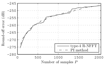
Figure 7: Round-off error versus number of samples $P$ for the type-4 R-NFFT method.

Finally, Fig. 8 shows the flop count of four methods: CG, GE, type-4 NFFT with $\eta=6$, and type-4 R-NFFT with $\eta=1$. Note that the last two methods roughly have the same flop count but, as shown in Fig. 4, the NFFT method is slightly above the GE, CG benchmark, while the R-NFFT method reaches it (Fig. 7).

Figure 8: Flop counts of four methods: GE, CG, type-4 NFFT with $\eta=6$, and type-4 R-NFFT with $\eta=1$.

VII Conclusions

We have presented non-iterative methods for the type 4 and 5 NFFTs in the one-dimensional case, which are significantly less expensive computationally that the state-of-the-art methods like the Conjugate Gradient. The methods are based on expressing the Lagrange formula in terms of nonuniform convolutions that can be efficiently evaluated using the type 1 and 2 NFFTs. The paper contains several numerical examples in which the proposed methods are compared with the Gaussian elimination (GE) and conjugate gradient (CG) methods in terms of round-off error and computational burden.

References

- [1] F. Andersson, R. Moses, and F. Natterer, “Fast Fourier methods for synthetic aperture radar imaging,” IEEE Transactions on Aerospace and Electronic Systems, vol. 48, no. 1, pp. 215–229, Jan 2012.
- [2] Susanne Kunis and Stefan Kunis, “The nonequispaced FFT on graphics processing units,” PAMM, vol. 12, no. 1, pp. 7–10, 2012.
- [3] L. Zhou, Z.H. Fan, L. Mo, R.S. Chen, and D.X. Wang, “A fast inverse NUFFT algorithm for computational electromagnetics,” in IEEE Antennas and Propagation Society International Symposium, July 2005, vol. 4B, pp. 160–163.
- [4] Jens Keiner, Stefan Kunis, and Daniel Potts, “Using NFFT 3—a software library for various nonequispaced fast Fourier transforms,” ACM Transactions on Mathematical Software, vol. 36, no. 4, pp. 1–30, aug 2009.
- [5] D. Potts, Schnelle Fourier-Transformationen für nichtäquidistante Daten und Anwendungen, Ph.D. thesis, Lübeck University, 2003.
- [6] John J Benedetto, Wavelets: mathematics and applications, vol. 13, chapter 12, CRC press, 1993.
- [7] A. J. W. Duijndam and M. A. Schonewille, “Nonuniform Fast Fourier Transform,” Geophysics, vol. 64, no. 2, pp. 539–551, 1999.
- [8] Alok Dutt and Vladimir Rokhlin, “Fast fourier transforms for nonequispaced data,” SIAM Journal on Scientific computing, vol. 14, no. 6, pp. 1368–1393, 1993.
- [9] Gene H. Golub and Charles F. Van Loan, Matrix Computations, The Johns Hopkins University Press, fourth edition, 2013.
- [10] Mariano Gasca and Thomas Sauer, “Polynomial interpolation in several variables,” Advances in Computational Mathematics, vol. 12, no. 4, pp. 377–410, 2001.
- [11] Prabhu Babu and Petre Stoica, “Spectral analysis of nonuniformly sampled data–a review,” Digital Signal Processing, vol. 20, no. 2, pp. 359–378, 2010.
- [12] Jeffrey A. Fessler and Bradley P. Sutton, “Nonuniform fast Fourier transform using mini-max interpolation,” IEEE Transactions on Signal Processing, vol. 51, pp. 560–574, Feb. 2003.
- [13] Amedeo Capozzoli, Claudio Curcio, Angelo Liseno, and Annalisa Riccardi, “Selecting parameters of type-3 NUFFTs to control accuracy in MoM methods,” in Antennas and Propagation (EuCAP), 2014 8th European Conference on. IEEE, 2014, pp. 1157–1161.
- [14] Q.H. Liu and N. Nguyen, “An accurate algorithm for nonuniform fast fourier transforms (NUFFT’s),” IEEE Microwave and Guided Wave Letters, vol. 8, no. 1, pp. 18–20, Jan 1998.
- [15] J. Selva, “An efficient Newton-type method for the computation of ML estimators in a Uniform Linear Array,” IEEE Transactions on Signal Processing, vol. 53, no. 6, pp. 2036–2045, June 2005.
- [16] June-Yub Lee and Leslie Greengard, “The type 3 nonuniform FFT and its applications,” Journal of Computational Physics, vol. 206, no. 1, pp. 1–5, 2005.
- [17] J. Selva, “FFT interpolation from nonuniform samples lying in a regular grid,” Signal Processing, IEEE Transactions on, vol. 63, no. 11, pp. 2826–2834, June 2015.
- [18] S. Kunis, Nonequispaced FFT, generalisation and inversion, Ph.D. thesis, Technisch-Naturwissenschaftlichen Fakultät, Universität zu Lübeck, 2006.