The monodromy representations of local systems associated with Lauricella’s $F_{D}$

Abstract.

We give the monodromy representations of local systems of twisted homology groups associated with Lauricella’s system $\mathcal{F}_{D}(a,b,c)$ of hypergeometric differential equations under mild conditions on parameters. Our representation is effective even in some cases when the system $\mathcal{F}_{D}(a,b,c)$ is reducible. We characterize invariant subspaces under our monodromy representations by the kernel or image of a natural map from a finite twisted homology group to locally finite one.

1. Introduction

There are several generalizations of the hypergeometric equation. Lauricella’s system $\mathcal{F}_{D}(a,b,c)$ of hypergeometric differential equations is regarded as the simplest system with multi-variables. It is regular singular and its rank is one more than the number of variables. Its singular locus $S$ is given in (2.3) and the fundamental group of its complement can be interpreted by the pure braid group. The monodromy representation of $\mathcal{F}_{D}(a,b,c)$ is studied by several authors under the non-integral condition on parameters:

(1.1) $$\alpha=(\alpha_{0},\alpha_{1},\dots,\alpha_{m},\alpha_{m+1},\alpha_{m+2})=(-c+\sum_{i=1}^{m}b_{i},-b_{1},\dots,-b_{m},c-a,a)\in(\mathbb{C}-\mathbb{Z})^{m+3},$$

where $m$ is the number of variables and the entries satisfy

(1.2) $$\sum_{i=0}^{m+2}\alpha_{i}=0;$$

cf. [DM], [IKSY], [OT], [M2], [T] and the references therein. As one of them, it is shown in [M2, Theorem 5.1] that circuit transformations are represented by the intersection form between twisted homology groups associated with the integral representation (2.1) of Euler type. The results in [M2] are based on a fact that the trivial vector bundle $\bigcup_{x\in U_{x}}H_{1}(T_{x},\mathcal{L}_{x}^{\alpha})$ is isomorphic to the local solution space to $\mathcal{F}_{D}(a,b,c)$ on $U_{x}$, where $x\in X=(\mathbb{P}^{1})^{m}-S$, $U_{x}(\subset X)$ is a simply connected small neighborhood of $x$, and $H_{1}(T_{x},\mathcal{L}_{x}^{\alpha})$ is the twisted homology group (refer to (3.1) for its definition).

In this paper, we generalize [M2, Theorem 5.1] by relaxing the condition (1.1) to

(1.3) $$(\alpha_{0},\alpha_{1},\dots,\alpha_{m},\alpha_{m+1},\alpha_{m+2})\notin\mathbb{Z}^{m+3}.$$

Note that there are at least two entries $\alpha_{i_{m+1}},\alpha_{i_{m+2}}\notin\mathbb{Z}$ by (1.2). Under this condition, we study the monodromy representations $\mathcal{M}^{\alpha}$ and $\mathcal{N}^{-\alpha}$ of local systems $\mathcal{H}_{1}^{lf}(\mathcal{L}^{\alpha})$ and $\mathcal{H}_{1}(\mathcal{L}^{-\alpha})$ with fibers $H_{1}^{lf}(T_{x},\mathcal{L}_{x}^{\alpha})$ and $H_{1}(T_{x},\mathcal{L}_{x}^{-\alpha})$, respectively, where $H_{1}^{lf}(T_{x},\mathcal{L}_{x}^{\alpha})$ is the locally finite twisted homology group and $H_{1}(T_{x},\mathcal{L}_{x}^{-\alpha})$ is given by the sign change $\alpha\mapsto-\alpha$ for $H_{1}(T_{x},\mathcal{L}_{x}^{\alpha})$. There is a natural linear map $\jmath_{h}^{\alpha}$ from $H_{1}(T_{x},\mathcal{L}_{x}^{\alpha})$ to $H_{1}^{lf}(T_{x},\mathcal{L}_{x}^{\alpha})$. It is known that this map is isomorphic under the condition (1.1). However, if there is an entry $\alpha_{i}$ of $\alpha$ such that $\alpha_{i}\in\mathbb{Z}$, then both of the kernel and the image of $\jmath_{h}^{\alpha}$ are proper subspaces. Thus it turns out that the monodromy representations $\mathcal{M}^{\alpha}$ and $\mathcal{N}^{-\alpha}$ of $\mathcal{H}_{1}^{lf}(\mathcal{L}^{\alpha})$ and $\mathcal{H}_{1}(\mathcal{L}^{-\alpha})$ are reducible in this case. In spite of this situation, the intersection form $\langle\;,\;\rangle$ between $H_{1}^{lf}(T_{x},\mathcal{L}_{x}^{\alpha})$ and $H_{1}(T_{x},\mathcal{L}_{x}^{-\alpha})$ is well-defined and perfect. We express circuit transformations as complex reflections with respect to the intersection form $\langle\;,\;\rangle$ in Theorem 5.4. We give their representation matrices with respect to bases of $H_{1}^{lf}(T_{x},\mathcal{L}_{x}^{\alpha})$ and $H_{1}(T_{x},\mathcal{L}_{x}^{-\alpha})$ in Corollary 6.1. We also give examples of representation matrices in the case of $m=3$, $\alpha_{0},\alpha_{1}\in\mathbb{Z}$ and $\alpha_{2}+\alpha_{3}\in\mathbb{Z}$ in §7.

We can define period matrices $\varPi_{c}^{lf}(\alpha,x)$ and $\varPi(\alpha,x)$ by the natural pairing between $H_{1}^{lf}(T_{x},\mathcal{L}_{x}^{\alpha})$ and $H^{1}_{c}(T_{x},\mathcal{L}_{x}^{\alpha})$, and that between $H_{1}(T_{x},\mathcal{L}_{x}^{\alpha})$ and $H^{1}(T_{x},\mathcal{L}_{x}^{\alpha})$, respectively, where $H^{1}(T_{x},\mathcal{L}_{x}^{\alpha})$ and $H^{1}_{c}(T_{x},\mathcal{L}_{x}^{\alpha})$ are the twisted cohomology group and that with compact support (refer to (8.1) for their definitions). Under the condition (1.1), each column vector of $\varPi_{c}^{lf}(\alpha,x)$ and $\varPi(\alpha,x)$ is a fundamental system of solutions to $\mathcal{F}_{D}(a^{\prime},b^{\prime},c^{\prime})$ for some $(a^{\prime},b^{\prime},c^{\prime})$, of which difference from $(a,b,c)$ is an integral vector. Under the condition (1.3), $\mathcal{M}^{\alpha}$ and $\mathcal{N}^{\alpha}$ can be regarded as the monodromy representations of $\varPi_{c}^{lf}(\alpha,x)$ and $\varPi(\alpha,x)$, though they do not always include a fundamental system of solutions to $\mathcal{F}_{D}(a,b,c)$. In general, the stalk of $\mathcal{H}_{1}^{lf}(\mathcal{L}^{\alpha})$ at $x$ cannot be regarded as the local solution space to $\mathcal{F}_{D}(a,b,c)$ around $x$ under only the condition (1.3). To identify these spaces, we suppose the condition

(1.4) $$\alpha_{i_{m}},\alpha_{i_{m+1}},\alpha_{i_{m+2}}\notin\mathbb{Z},\ \quad\alpha_{i_{m+1}}+\alpha_{i_{m+2}}\neq 0,$$

and the non negative-integral condition (8.3). Under these conditions, the monodromy representation $\mathcal{M}^{\alpha}$ can be regarded as that of $\mathcal{F}_{D}(a,b,c)$. Similarly, under the conditions (1.4) and (8.5), the monodromy representation $\mathcal{N}^{-\alpha}$ can be regarded as that of $\mathcal{F}_{D}(-a,-b,-c)$.

2. Lauricella’s system $F_{D}$

Lauricella’s hypergeometric series $F_{D}(a,b,c;x)$ is defined by

$$F_{D}(a,b,c;x)=\sum_{n\in\mathbb{N}^{m}}\frac{(a,\sum_{i=1}^{m}n_{i})\prod_{i=1}^{m}(b_{i},n_{i})}{(c,\sum_{i=1}^{m}n_{i})\prod_{i=1}^{m}(1,n_{i})}\prod_{i=1}^{m}x_{i}^{n_{i}},$$

where $x_{1},\dots,x_{m}$ are complex variables with $|x_{i}|<1$ $(1\leq i\leq m)$, $a$, $b=(b_{1},\dots,b_{m})$ and $c$ are complex parameters, $c\notin-\mathbb{N}=\{0,-1,-2,\dots\}$, and $(b_{i},n_{i})=b_{i}(b_{i}+1)\cdots(b_{i}+n_{i}-1)$. It admits an Euler type integral representation:

(2.1) $$F_{D}(a,b,c;x)=\frac{\mathit{\Gamma}(c)}{\mathit{\Gamma}(a)\mathit{\Gamma}(c\!-\!a)}\int_{1}^{\infty}u(t,x)\frac{dt}{t\!-\!1},\quad u(t,x)=t^{\sum_{i}b_{i}-c}(t\!-\!1)^{c-a}\prod_{i=1}^{m}(t\!-\!x_{i})^{-b_{i}},$$

where the parameters $a$ and $c$ satisfy $\mathrm{Re}(c)>\mathrm{Re}(a)>0$.

The differential operators

$$x_{i}(1-x_{i})\partial_{i}^{2}+(1-x_{i})\sum\limits_{1\leq j\leq m}^{j\neq i}x_{j}\partial_{i}\partial_{j}+[c-(a+b_{i}+1)x_{i}]\partial_{i}-b_{i}\sum\limits_{1\leq j\leq m}^{j\neq i}x_{j}\partial_{j}-ab_{i},$$

(2.2) $$(1\leq i\leq m)$$

$$(x_{i}-x_{j})\partial_{i}\partial_{j}-b_{j}\partial_{i}+b_{i}\partial_{j},\hskip 85.35826pt(1\leq i<j\leq m)$$

annihilate the series $F_{D}(a,b,c;x)$, where $\partial_{i}=\dfrac{\partial}{\partial x_{i}}$. Lauricella’s system $\mathcal{F}_{D}(a,b,c)$ is defined by the ideal generated by these operators in the Weyl algebra $\mathbb{C}[x_{1},\dots,x_{m}]\langle\partial_{1},\dots,\partial_{m}\rangle$. Though the series $F_{D}(a,b,c;x)$ is not defined when $c\in-\mathbb{N}=\{0,-1,-2,\dots\}$, the system $\mathcal{F}_{D}(a,b,c)$ is valid even in this case. It is a regular holonomic system of rank $m+1$ with singular locus

(2.3) $$S=\big{\{}x\in\mathbb{C}^{m}\Big{|}\prod_{i=1}^{m}[x_{i}(1-x_{i})]\prod_{1\leq i<j\leq m}(x_{i}-x_{j})=0\big{\}}\cup(\cup_{i=1}^{\infty}\{x_{i}=\infty\})\subset(\mathbb{P}^{1})^{m}.$$

We set

$$X=(\mathbb{P}^{1})^{m}-S=\big{\{}(x_{1},\dots,x_{m})\in\mathbb{C}^{m}\mid\prod_{0\leq i<j\leq m+1}(x_{j}-x_{i})\neq 0\big{\}},$$

where $x_{0}=0$ and $x_{m+1}=1$. We introduce a notation

$$\tilde{x}=(x_{0},x_{1},\dots,x_{m},x_{m+1},x_{m+2})=(0,x_{1},\dots,x_{m},1,\infty)=(0,x,1,\infty)$$

for $x\in X$. Let $\mathrm{Sol}_{x}(a,b,c)$ be the vector space of solutions to $\mathcal{F}_{D}(a,b,c)$ on a small simply connected neighborhood $U(\subset X)$ of $x$. It is called the local solution space to $\mathcal{F}_{D}(a,b,c)$ around $x$, and it is $(m+1)$-dimensional. If the improper integral

(2.4) $$\int_{x_{i}}^{x_{j}}u(t,x)\frac{dt}{t\!-\!1}\quad(0\leq i<j\leq m+2)$$

converges, then it gives an element of $\mathrm{Sol}_{x}(a,b,c)$.

We set

$$\mathfrak{X}=\Big{\{}(x,t)\in\mathbb{C}^{m}\times\mathbb{C}\;\Big{|}\;x\in X,\ \prod_{i=0}^{m+1}(t-x_{i})\neq 0\big{\}},$$

and

$$T_{x}=\Big{\{}t\in\mathbb{C}\;\Big{|}\prod_{i=0}^{m+1}(t-x_{i})\neq 0\Big{\}}=\mathbb{C}-\{0,x_{1},\dots,x_{m},1\}$$

for any fixed $x\in X$. Note that $T_{x}$ is the preimage of $x$ under the projection

$$\mathrm{pr}:\mathfrak{X}\ni(x,t)\mapsto x\in X.$$

3. Twisted homology groups

In this section, we prepare facts about twisted homology groups associated with the Euler type integral (2.1) for our study.

Throughout this paper, we assume the conditions (1.2) and (1.3) on $\alpha$. We put

$$\lambda=(\lambda_{0},\lambda_{1},\dots,\lambda_{m},\lambda_{m+1},\lambda_{m+2}),\qquad\lambda_{i}=\exp(2\pi\sqrt{-1}\alpha_{i})\quad(0\leq i\leq m+2).$$

Note that $\prod_{i=0}^{m+2}\lambda_{i}=1$. By regarding $\lambda_{i}$ as indeterminants, we have the rational function field $\mathbb{C}(\lambda)=\mathbb{C}(\lambda_{0},\lambda_{1},\dots,\lambda_{m},\lambda_{m+1})$. Let $\mathcal{L}^{\alpha}$ be a locally constant sheaf on $\mathfrak{X}$ defined by a multi-valued function

$$u(t,x)=\prod_{i=0}^{m+1}(t-x_{i})^{\alpha_{i}}=t^{\alpha_{0}}(t-x_{1})^{\alpha_{1}}\cdots(t-x_{m})^{\alpha_{m}}(t-1)^{\alpha_{m+1}},$$

and $\mathcal{L}_{x}^{\alpha}$ be that on $T_{x}$ defined by its restriction $u_{x}=u_{x}(t)$ to $T_{x}$. For a fixed $x\in X$, we define a vector space

$$\mathcal{C}_{k}(u_{x})=\Big{\{}\sum_{\nu}w_{\nu}\cdot(\tau_{\nu},u_{x}|_{\tau_{\nu}})\mid w_{\nu}\in\mathbb{C}(\lambda)\Big{\}}$$

over $\mathbb{C}(\lambda)$, where the sum is finite, $\tau_{\nu}$ is a $k$-chain in $T_{x}$ and $u_{x}|_{\tau_{\nu}}$ is a branch of $u_{x}$ on $\tau_{\nu}$. We define a twisted homology group as a quotient space

(3.1) $$H_{1}(T_{x},\mathcal{L}_{x}^{\alpha})=\ker(\partial_{u}:\mathcal{C}_{1}(u_{x})\to\mathcal{C}_{2}(u_{x}))/\partial_{u}(\mathcal{C}_{0}(u_{x})),$$

where $\partial_{u}$ is a boundary operator defined by

$$\partial_{u}(\tau_{\nu},u_{x}|_{\tau_{\nu}})=(\partial\tau_{\nu},(u_{x}|_{\tau_{\nu}})|_{\partial\tau_{\nu}}).$$

Similarly we have a locally finite twisted homology group

(3.2) $$H_{1}^{lf}(T_{x},\mathcal{L}_{x}^{\alpha})=\ker(\partial_{u}:\mathcal{C}^{lf}_{1}(u_{x})\to\mathcal{C}^{lf}_{2}(u_{x}))/\partial_{u}(\mathcal{C}^{lf}_{0}(u_{x})),$$

where $\mathcal{C}^{lf}_{k}(u_{x})$ is defined by extending finite sums to locally finite sums for $\mathcal{C}_{k}(u_{x})$.

The dimensions of $H_{1}^{lf}(T_{x},\mathcal{L}_{x}^{\alpha})$ and $H_{1}(T_{x},\mathcal{L}_{x}^{\alpha})$ are equal to $-\chi(T_{x})$ by [C, Theorem 1], where $\chi(T_{x})$ is the Euler number of $T_{x}$. Thus we have the following.

Fact 3.1.

$$\dim H_{1}(T_{x},\mathcal{L}_{x}^{\alpha})=\dim H_{1}^{lf}(T_{x},\mathcal{L}_{x}^{\alpha})=m+1.$$

We have a natural map

(3.3) $$\jmath_{h}^{\alpha}:H_{1}(T_{x},\mathcal{L}_{x}^{\alpha})\to H_{1}^{lf}(T_{x},\mathcal{L}_{x}^{\alpha})$$

by regarding a finite sum as a locally finite sum. This map is isomorphic under the condition (1.1) and its inverse $\mathrm{reg}$ is called the regularization. However, under our assumption (1.3), it does not hold in general.

Lemma 3.2.

If there exists a parameter $\alpha_{i}\in\mathbb{Z}$ then the map $\jmath_{h}^{\alpha}$ is not isomorphic. Even in this case, we have an isomorphism

$$\mathrm{reg}:\mathrm{Im}(\jmath_{h}^{\alpha})\to H_{1}(T_{x},\mathcal{L}_{x}^{\alpha})/\ker(\jmath_{h}^{\alpha}).$$

Proof..

Suppose that $\alpha_{i}$ is an integer. Let $\odot_{i}$ be an annulus

$$\{t\in T_{x}\mid 0<|t-x_{i}|\leq\varepsilon\},$$

and $\circlearrowleft_{i}$ be its boundary, where $\varepsilon$ is a small positive real number. For the case $i=m+2$, they are regarded as

$$\odot_{m+2}=\{t\in T_{x}\mid|t|\geq 1/\varepsilon\},\quad\circlearrowleft_{m+2}=\{t\in T_{x}\mid|t|=1/\varepsilon\}.$$

Since $u_{x}(t)$ is single-valued on $\odot_{i}$, we can regard $(\odot_{i},u_{x}(t)|_{\odot_{i}})$ as an element of $\mathcal{C}^{lf}_{2}(u_{x})$. Thus its image $(\circlearrowleft_{i},u_{x}(t)|_{\circlearrowleft_{i}})$ under $\partial_{u}$ is $0$ as an element of $H_{1}^{lf}(T_{x},\mathcal{L}_{x}^{\alpha})$. However, we cannot regard $(\odot_{i},u_{x}(t)|_{\odot_{i}})$ as an element of $\mathcal{C}_{2}(u_{x})$, since $\odot_{i}$ does not admit an expression as a finite union of $2$-simplexes. In fact, we will show that $(\circlearrowleft_{i},u_{x}(t)|_{\circlearrowleft_{i}})$ is not $0$ as an element of $H_{1}(T_{x},\mathcal{L}_{x}^{\alpha})$ in Proposition 3.4. It is elementary that $H_{1}(T_{x},\mathcal{L}_{x}^{\alpha})/\ker(\jmath_{h}^{\alpha})$ is isomorphic to $\mathrm{Im}(\jmath_{h}^{\alpha})$. $\square$

We give bases of $H_{1}^{lf}(T_{x},\mathcal{L}_{x}^{\alpha})$ and $H_{1}(T_{x},\mathcal{L}_{x}^{-\alpha})$. Put

(3.4) $$r=\#\{0\leq i\leq m+2\mid\alpha_{i}\in\mathbb{Z}\},$$

and suppose that

(3.5) $$\alpha_{i_{0}},\alpha_{i_{1}},\dots,\alpha_{i_{r-1}}\in\mathbb{Z},\quad\alpha_{i_{r}},\dots,\alpha_{i_{m+1}},\alpha_{i_{m+2}}\notin\mathbb{Z},$$

and the corresponding points $x_{i}$ $(i=0,\dots,m+2)$ are aligned

(3.6) $$x_{i_{0}}<x_{i_{1}}<\cdots<x_{i_{m}}<x_{i_{m+1}}<x_{i_{m+2}},$$

where

$$\left\{\begin{array}[]{cccc}i_{m+2}=m+2,&x_{i_{m+2}}=\infty&\textrm{if}&\alpha_{m+2}\notin\mathbb{Z},\\ i_{0}=m+2,&x_{i_{0}}=-\infty&\textrm{if}&\alpha_{m+2}\in\mathbb{Z}.\\ \end{array}\right.$$

Let $\imath$ be an element of the symmetric group $\mathfrak{S}_{m+3}$ satisfying

(3.7) $$\imath(i_{0})=0,\ \imath(i_{1})=1,\ \dots,\ \imath(i_{m})=m,\ \imath(i_{m+1})=m+1,\ \imath(i_{m+2})=m+2.$$

Then it satisfies $\imath^{-1}(p)=i_{p}$ for $0\leq p\leq m+2$. We fix these $x_{1},\dots,x_{m}$. Suppose that the circle

$$\circlearrowleft_{i}=\{t\in T_{x}\mid|t-x_{i}|=\varepsilon\}\quad(0\leq i\leq m+1),$$

is positively oriented with terminal $\hat{x}_{i}=x_{i}+\sqrt{-1}\varepsilon$ for $0\leq i\leq m+1$, see Figure 1, and

$$\circlearrowleft_{m+2}=\{t\in T_{x}\mid|t|=1/\varepsilon\}$$

is negatively oriented with terminal $\hat{x}_{m+2}=\sqrt{-1}/\varepsilon$.

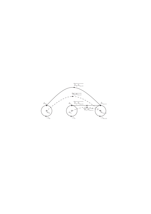
Figure 1. Twisted cycles

We define twisted cycles by

(3.8) $$\ell_{k}^{\alpha} =(\overleftarrow{\;x_{i_{k}}{x_{i_{m+1}}}},u_{x})\in H_{1}^{lf}(T_{x},\mathcal{L}_{x}^{\alpha}),$$

(3.9) $$\gamma_{k}^{-\alpha} =(\lambda^{-1}_{i_{k}}-1)(\overleftarrow{\;{\hat{x}_{i_{k}}}{\hat{x}_{i_{m+1}}}},u^{-1}_{x})-(\circlearrowleft_{i_{k}},u^{-1}_{x})+\frac{\lambda^{-1}_{i_{k}}-1}{\lambda^{-1}_{i_{m+1}}-1}(\circlearrowleft_{i_{m+1}},u^{-1}_{x})\in H_{1}(T_{x},\mathcal{L}_{x}^{-\alpha}),$$

for $0\leq k\leq m$, where we take and fix a branch $u_{x}$ of $u_{x}(t)$ on the upper half space $\mathbb{H}\subset T_{x}$, and $\overleftarrow{\;x_{i_{k}}{x_{i_{m+1}}}}$ and $\overleftarrow{\;{\hat{x}_{i_{k}}}{\hat{x}_{i_{m+1}}}}$ are an oriented arc in $\mathbb{H}$ from $x_{i_{m+1}}$ to $x_{i_{k}}$ and that from $\hat{x}_{i_{m+1}}$ to $\hat{x}_{i_{k}}$, respectively, see Figure 1. Note that they are well-defined under the assumption (3.5) and that

$$\gamma_{k}^{-\alpha}=(\circlearrowleft_{i_{k}},u^{-1}_{x})\quad(0\leq k\leq r-1)$$

by $1-\lambda^{-1}_{i_{k}}=0$ for $0\leq k\leq r-1$.

Definition 3.3 ([AK],[Y]).

The intersection form between $H_{1}^{lf}(T_{x},\mathcal{L}_{x}^{\alpha})$ and $H_{1}(T_{x},\mathcal{L}_{x}^{-\alpha})$ is defined by

(3.10) $$\langle\ell^{\alpha},\gamma^{-\alpha}\rangle=\sum_{\mu,\nu}\sum_{t^{\sigma}_{\tau}\in\sigma_{\mu}\cap\tau_{\nu}}(z_{\mu}\cdot w_{\nu})\cdot[\sigma_{\mu},\tau_{\nu}]_{t^{\mu}_{\nu}}\cdot(u_{x}(t^{\mu}_{\nu})|_{\sigma_{\mu}}\cdot u_{x}^{-1}(t^{\mu}_{\nu})|_{\tau_{\nu}})\in\mathbb{C}(\lambda),$$

where

$$\ell^{\alpha}=\sum_{\mu}z_{\mu}\cdot(\sigma_{\mu},u_{x}|_{\sigma_{\mu}})\in H_{1}^{lf}(T_{x},\mathcal{L}_{x}^{\alpha}),\quad\gamma^{-\alpha}=\sum_{\nu}w_{\nu}\cdot(\tau_{\nu},u_{x}^{-1}|_{\tau_{\nu}})\in H_{1}(T_{x},\mathcal{L}_{x}^{-\alpha}),$$

the formal sum for $\mu$ is locally finite, the formal sum for $\nu$ is finite, and $1$-chains $\sigma_{\mu}$ and $\tau_{\nu}$ intersect transversally at most one point $t^{\mu}_{\nu}$ with the topological intersection number $[\sigma_{\mu},\tau_{\nu}]_{t^{\mu}_{\nu}}=\pm 1$.

Proposition 3.4.

Under the condition (1.3), the intersection form $\langle\;,\;\rangle$ is perfect, and the twisted cycles $\ell_{0}^{\alpha},\ell_{1}^{\alpha},\dots,\ell_{m}^{\alpha}$ and $\gamma_{0}^{-\alpha},\gamma_{1}^{-\alpha},\dots,\gamma_{m}^{-\alpha}$ are bases of $H_{1}^{lf}(T_{x},\mathcal{L}_{x}^{\alpha})$ and $H_{1}(T_{x},\mathcal{L}_{x}^{-\alpha})$, respectively.

Proof..

We compute the intersection matrix $H=\big{(}\langle\ell_{k}^{\alpha},\gamma_{k^{\prime}}^{-\alpha}\rangle\big{)}_{0\leq k,k^{\prime}\leq m}$. The locally finite chain $\overleftarrow{\;x_{i_{0}}x_{i_{m+1}}}$ and finite chains consisting of $\gamma_{0}^{-\alpha}$ intersect at two points $t_{0}^{0}$ and $t_{m+1}^{0}$ on $\circlearrowleft_{i_{0}}$ and on $\circlearrowleft_{i_{m}}$, respectively. The topological intersection numbers are

$$[\overleftarrow{\;x_{i_{0}}x_{i_{m+1}}},\circlearrowleft_{i_{0}}]_{t_{0}^{0}}=-1,\quad[\overleftarrow{\;x_{i_{0}}x_{i_{m+1}}},\circlearrowleft_{i_{m+1}}]_{t_{m+1}^{0}}=1,$$

and the products of branches of $u_{x}(t)$ and $1/u_{x}(t)$ at $t_{0}^{0}$ and $t_{m+1}^{0}$ are

$$u_{x}(t_{0}^{0})\cdot\frac{1}{u_{x}(t_{0}^{0})}=\lambda_{i_{0}}^{-1},\quad u_{x}(t_{m+1}^{0})\cdot\frac{1}{u_{x}(t_{m+1}^{0})}=1.$$

By considering coefficients, we have

$$\langle\ell_{0}^{\alpha},\gamma_{0}^{-\alpha}\rangle=\lambda_{i_{0}}^{-1}+\frac{\lambda_{i_{0}}^{-1}-1}{\lambda_{i_{m+1}}^{-1}-1}=\frac{\lambda_{i_{0}}\lambda_{i_{m+1}}-1}{\lambda_{i_{0}}(\lambda_{i_{m+1}}-1)}=1+\frac{\lambda_{i_{0}}-1}{\lambda_{i_{0}}(\lambda_{i_{m+1}}-1)}.$$

Similarly, we have

$$\langle\ell_{0}^{\alpha},\gamma_{k}^{-\alpha}\rangle=\frac{\lambda_{i_{k}}-1}{\lambda_{i_{k}}(\lambda_{i_{m+1}}-1)},\quad\langle\ell_{k}^{\alpha},\gamma_{0}^{-\alpha}\rangle=\frac{(\lambda_{i_{0}}-1)\lambda_{i_{m+1}}}{\lambda_{i_{0}}(\lambda_{i_{m+1}}-1)}$$

for $1\leq k\leq m$. Hence we have

(3.11) $$H=I_{m+1}+\frac{1}{\lambda_{i_{m+1}}-1}\begin{pmatrix}1&1&\cdots&1\\ \lambda_{i_{m+1}}&1&\cdots&1\\ \vdots&\ddots&\ddots&\vdots\\ \lambda_{i_{m+1}}&\cdots&\lambda_{i_{m+1}}&1\end{pmatrix}\mathrm{diag}\big{(}\overbrace{0,\dots,0}^{r},\frac{\lambda_{i_{r}}-1}{\lambda_{i_{r}}},\dots,\frac{\lambda_{i_{m}}-1}{\lambda_{i_{m}}}\big{)},$$

where $I_{m+1}$ is the unit matrix of size $m+1$, and $\mathrm{diag}(z_{0},\dots,z_{m})$ denotes the diagonal matrix with diagonal entries $z_{0},\dots,z_{m}$. Since its determinant is

$$\frac{1-\lambda_{i_{m+2}}}{1-\lambda_{i_{m+1}}^{-1}}\neq 0,$$

$\ell_{0}^{\alpha},\dots,\ell_{m}^{\alpha}$ and $\gamma_{0}^{-\alpha},\dots,\gamma_{m}^{-\alpha}$ are bases of $H_{1}^{lf}(T_{x},\mathcal{L}_{x}^{\alpha})$ and $H_{1}(T_{x},\mathcal{L}_{x}^{-\alpha})$, and the intersection form is perfect. $\square$

Remark 3.5.

We extend the notations in (3.8) and (3.9) to $k=m+1,m+2$. It is obvious that $\ell^{\alpha}_{m+1}=0$, $\gamma^{-\alpha}_{m+1}=0$. Since

$$\langle\ell^{\alpha}_{m+2},\gamma^{-\alpha}_{k}\rangle=\frac{\lambda_{i_{k}}^{-1}-1}{\lambda_{i_{m+1}}^{-1}-1}\cdot\lambda_{i_{m+1}}^{-1},\quad\langle\ell^{\alpha}_{k},\gamma^{-\alpha}_{m+1}\rangle=\frac{\lambda_{i_{m+2}}^{-1}-1}{\lambda_{i_{m+1}}^{-1}-1},$$

the cycles $\ell^{\alpha}_{m+2}$ and $\gamma^{-\alpha}_{m+2}$ are expressed as linear combinations

$$\ell^{\alpha}_{m+2}=\mathbf{e}_{m+2}\cdot\begin{pmatrix}\ell^{\alpha}_{0}\\ \ell^{\alpha}_{1}\\ \vdots\\ \ell^{\alpha}_{m}\end{pmatrix},\quad\gamma^{-\alpha}_{m+2}=\big{(}\gamma^{-\alpha}_{0},\gamma^{-\alpha}_{1},\dots,\gamma^{-\alpha}_{m}\big{)}\cdot\mathbf{e}_{m+2}^{*},$$

(3.12) $$\mathbf{e}_{m+2}=\frac{-\lambda_{i_{m+2}}}{\lambda_{i_{m+2}}-1}\Big{(}(\lambda_{i_{0}}-1),\lambda_{i_{0}}(\lambda_{i_{1}}-1),\cdots,\lambda_{i_{0}}\lambda_{i_{1}}\cdots\lambda_{i_{m-1}}(\lambda_{i_{m}}-1)\Big{)},$$

(3.17) $$\mathbf{e}_{m+2}^{*}=\left(\begin{array}[]{r}\lambda_{i_{0}}\lambda_{i_{1}}\cdots\lambda_{i_{m}}\\ \lambda_{i_{1}}\cdots\lambda_{i_{m}}\\ \vdots\\ \lambda_{i_{m}}\end{array}\right).$$

Their intersection number is

$$\langle\ell^{\alpha}_{m+2},\gamma^{-\alpha}_{m+2}\rangle=\frac{\lambda_{i_{m+1}}\lambda_{i_{m+2}}-1}{(\lambda_{i_{m+1}}-1)\lambda_{i_{m+2}}}=1+\frac{\lambda_{i_{m+2}}-1}{(\lambda_{i_{m+1}}-1)\lambda_{i_{m+2}}}.$$

4. Local systems

We take a base point $\dot{x}\in X$ so that

$$(\dot{x}_{0},\dot{x}_{1},\dots,\dot{x}_{m},\dot{x}_{m+1},\dot{x}_{m+2})=(0,\dot{x}_{1},\dots,\dot{x}_{m},1,\infty)$$

are aligned as in (3.6) for a fixed parameter $\alpha$ satisfying (3.5). We set

$$\mathbb{C}_{p}(\dot{x})=\{(\dot{x}_{1},\dots,\dot{x}_{p-1},x_{p},\dot{x}_{p+1},\dots,\dot{x}_{m})\mid x_{p}\in\mathbb{C}\}\quad(1\leq p\leq m),$$

which are lines in $\mathbb{C}^{m}$ passing through $\dot{x}$. For distinct indexes $1\leq p\leq m$ and $0\leq q\leq m+1$, let $\rho_{pq}$ be a loop in $X\cap\mathbb{C}_{p}(\dot{x})$ starting from $x_{p}=\dot{x}_{p}$, approaching to $\dot{x}_{q}$ via the upper half space in $\mathbb{C}_{p}(\dot{x})$, turning $\dot{x}_{q}$ once positively, and tracing back to $\dot{x}_{p}$.

Fact 4.1.

The fundamental group $\pi_{1}(X,\dot{x})$ is generated by the loops $\rho_{pq}$, where $0\leq p<q\leq m+1$, $(p,q)\neq(0,m+1)$, and $\rho_{0p}$ is regarded as the loop $\rho_{p0}$ in $X\cap\mathbb{C}_{p}(\dot{x})$.

By the local triviality of the spaces $H_{1}^{lf}(T_{x},\mathcal{L}_{x}^{\alpha})$, $H_{1}(T_{x},\mathcal{L}_{x}^{\alpha})$, $H_{1}(T_{x},\mathcal{L}_{x}^{-\alpha})$, $H_{1}^{lf}(T_{x},\mathcal{L}_{x}^{-\alpha})$, we have the local systems

$$\mathcal{H}_{1}^{lf}(\mathcal{L}^{\alpha})=\bigcup_{x\in X}H_{1}^{lf}(T_{x},\mathcal{L}_{x}^{\alpha}),\quad\mathcal{H}_{1}(\mathcal{L}^{\alpha})=\bigcup_{x\in X}H_{1}(T_{x},\mathcal{L}_{x}^{\alpha}),$$

$$\mathcal{H}_{1}(\mathcal{L}^{-\alpha})=\bigcup_{x\in X}H_{1}(T_{x},\mathcal{L}_{x}^{-\alpha}),\quad\mathcal{H}_{1}^{lf}(\mathcal{L}^{-\alpha})=\bigcup_{x\in X}H_{1}^{lf}(T_{x},\mathcal{L}_{x}^{-\alpha}),$$

over $X$.

Proposition 4.2.

1. The natural map $\jmath_{h}^{\alpha}:H_{1}(T_{x},\mathcal{L}_{x}^{\alpha})\to H_{1}^{lf}(T_{x},\mathcal{L}_{x}^{\alpha})$ commutes with horizontal deformations in $\mathcal{H}_{1}^{lf}(\mathcal{L}^{\alpha})$.

2. The intersection form $\langle\;,\;\rangle$ between $H_{1}^{lf}(T_{x},\mathcal{L}_{x}^{\alpha})$ and $H_{1}(T_{x},\mathcal{L}_{x}^{-\alpha})$ is stable under horizontal deformations in $\mathcal{H}_{1}^{lf}(\mathcal{L}^{\alpha})$ and $\mathcal{H}_{1}(\mathcal{L}^{-\alpha})$.

Proof..

(1) It is obvious by the definition of $\jmath_{h}^{\alpha}$.

(2) Note that the intersection matrix $H$ in (3.11) is independent of $x\in X$. $\square$

5. Monodromy representations

Let $U$ be a small simply connected neighborhood of $\dot{x}$ contained in $X$. We set four trivial vector bundles

$$\begin{array}[]{ll}V^{lf}(\mathcal{L}^{\alpha})=\bigcup\limits_{x\in U}H_{1}^{lf}(T_{x},\mathcal{L}_{x}^{\alpha})\subset\mathcal{H}_{1}^{lf}(\mathcal{L}^{\alpha}),&V(\mathcal{L}^{\alpha})=\bigcup\limits_{x\in U}H_{1}(T_{x},\mathcal{L}_{x}^{\alpha})\subset\mathcal{H}_{1}(\mathcal{L}^{\alpha}),\\ V(\mathcal{L}^{-\alpha})=\bigcup\limits_{x\in U}H_{1}(T_{x},\mathcal{L}_{x}^{-\alpha})\subset\mathcal{H}_{1}(\mathcal{L}^{-\alpha}),&V^{lf}(\mathcal{L}^{-\alpha})=\bigcup\limits_{x\in U}H_{1}^{lf}(T_{x},\mathcal{L}_{x}^{-\alpha})\subset\mathcal{H}_{1}^{lf}(\mathcal{L}^{-\alpha}).\end{array}$$

We identify sections of $V^{lf}(\mathcal{L}^{\alpha})$, $V(\mathcal{L}^{\alpha})$, $V(\mathcal{L}^{-\alpha})$ and $V^{lf}(\mathcal{L}^{-\alpha})$ with elements of $H_{1}^{lf}(T_{x},\mathcal{L}_{x}^{\alpha})$, $H_{1}(T_{x},\mathcal{L}_{x}^{\alpha})$, $H_{1}(T_{x},\mathcal{L}_{x}^{-\alpha})$ and $H_{1}^{lf}(T_{x},\mathcal{L}_{x}^{-\alpha})$ for a fixed element $x\in U$.

A loop $\rho$ with terminal $\dot{x}$ in $X$ induces $\mathbb{C}$-linear isomorphisms

$$\mathcal{M}^{\alpha}_{\rho} :V^{lf}(\mathcal{L}^{\alpha})\ni\ell^{\alpha}\mapsto\rho_{*}\ell^{\alpha}\in V^{lf}(\mathcal{L}^{\alpha}),$$

$$\mathcal{N}^{\alpha}_{\rho} :V(\mathcal{L}^{\alpha})\ni\gamma^{\alpha}\mapsto\rho_{*}\gamma^{\alpha}\in V(\mathcal{L}^{\alpha}),$$

$$\mathcal{N}^{-\alpha}_{\rho} :V(\mathcal{L}^{-\alpha})\ni\gamma^{-\alpha}\mapsto\rho_{*}\gamma^{-\alpha}\in V(\mathcal{L}^{-\alpha}),$$

$$\mathcal{M}^{-\alpha}_{\rho} :V^{lf}(\mathcal{L}^{-\alpha})\ni\ell^{-\alpha}\mapsto\rho_{*}\ell^{-\alpha}\in V^{lf}(\mathcal{L}^{-\alpha}),$$

where $\ell^{\alpha}\in H_{1}^{lf}(T_{x},\mathcal{L}_{x}^{\alpha})$, $\gamma^{\alpha}\in H_{1}(T_{x},\mathcal{L}_{x}^{\alpha})$, $\gamma^{-\alpha}\in H_{1}(T_{x},\mathcal{L}_{x}^{-\alpha})$ and $\ell^{-\alpha}\in H_{1}^{lf}(T_{x},\mathcal{L}_{x}^{-\alpha})$ are regarded as sections of $V^{lf}(\mathcal{L}^{\alpha})$, $V(\mathcal{L}^{\alpha})$, $V(\mathcal{L}^{-\alpha})$ and $V^{lf}(\mathcal{L}^{-\alpha})$, and $\rho_{*}\ell^{\alpha}$, $\rho_{*}\gamma^{\alpha}$ $\rho_{*}\gamma^{-\alpha}$, $\rho_{*}\ell^{-\alpha}$ are their continuations along the loop $\rho$. They are called circuit transformations along $\rho$. The map $\rho\mapsto\mathcal{M}^{\alpha}_{\rho}$ induces a homomorphism

$$\mathcal{M}^{\alpha}:\pi_{1}(X,\dot{x})\ni\rho\mapsto\mathcal{M}^{\alpha}_{\rho}\in GL(V^{lf}(\mathcal{L}^{\alpha})),$$

which is called the monodromy representation. Similarly, we have the monodromy representations

$$\mathcal{N}^{\alpha} :\pi_{1}(X,\dot{x})\to GL(V(\mathcal{L}^{\alpha})),$$

$$\mathcal{N}^{-\alpha} :\pi_{1}(X,\dot{x})\to GL(V(\mathcal{L}^{-\alpha})),$$

$$\mathcal{M}^{-\alpha} :\pi_{1}(X,\dot{x})\to GL(V^{lf}(\mathcal{L}^{-\alpha})).$$

Proposition 5.1.

Suppose that the condition (1.3). If there exists a parameter $\alpha_{i}\in\mathbb{Z}$ then the monodromy representations $\mathcal{M}^{\alpha}$, $\mathcal{N}^{\alpha}$, $\mathcal{N}^{-\alpha}$ and $\mathcal{M}^{-\alpha}$ are reducible. Their proper invariant subspaces are $\mathrm{im}(\jmath_{h}^{\alpha})$, $\ker(\jmath_{h}^{\alpha})$, $\ker(\jmath_{h}^{-\alpha})$ and $\mathrm{im}(\jmath_{h}^{-\alpha})$, respectively, where the natural map $\jmath_{h}^{\alpha}$ is given in (3.3).

Proof..

By Lemma 3.2, the image $\mathrm{im}(\jmath_{h}^{\alpha})$ and the kernel $\ker(\jmath_{h}^{\alpha})$ of $\jmath_{h}^{\alpha}$ are proper subspaces. By Proposition 4.2 (1), they are invariant under any circuit transformations. Hence $\mathcal{M}^{\alpha}$ and $\mathcal{N}^{\alpha}$ are reducible. For the reducibility of $\mathcal{N}^{-\alpha}$ and $\mathcal{M}^{-\alpha}$, use the sign change $\alpha\mapsto-\alpha$. $\square$

Since $\mathcal{M}^{-\alpha}$ and $\mathcal{N}^{\alpha}$ are obtained from the sign change $\alpha\mapsto-\alpha$ for $\mathcal{M}^{\alpha}$ and $\mathcal{N}^{-\alpha}$, we mainly treat $\mathcal{M}^{\alpha}$ and $\mathcal{N}^{-\alpha}$.

Proposition 5.2.

1. The intersection form is invariant under the monodromy representations, that is

   $$\langle\mathcal{M}_{\rho}^{\alpha}(\ell^{\alpha}),\mathcal{N}_{\rho}^{-\alpha}(\gamma^{-\alpha})\rangle=\langle\ell^{\alpha},\gamma^{-\alpha}\rangle,$$

   where $\rho$ is a loop in $X$ with terminal $\dot{x}$, and $\ell^{\alpha}$ and $\gamma^{-\alpha}$ are sections in $V^{lf}(\mathcal{L}^{\alpha})$ and $V(\mathcal{L}^{-\alpha})$.

2. If $\beta$ is an eigenvalue of $\mathcal{M}_{\rho}^{\alpha}$, then $\beta^{-1}$ is an eigenvalue of $\mathcal{N}_{\rho}^{-\alpha}$.

3. Let $\ell^{\alpha}$ be a $\beta$-eigenvector of $\mathcal{M}_{\rho}^{\alpha}$, and $\gamma^{-\alpha}$ be a $\beta^{\prime}$-eigenvector of $\mathcal{N}_{\rho}^{-\alpha}$. If $\beta\beta^{\prime}\neq 1$ then $\langle\ell^{\alpha},\gamma^{-\alpha}\rangle=0$. If $\langle\ell^{\alpha},\gamma^{-\alpha}\rangle\neq 0$ then $\beta\beta^{\prime}=1$.

Proof..

(1) This property is a natural consequence from Proposition 4.2 (2).

(2) Since $\mathcal{M}_{\rho}^{\alpha}$ is invertible, $\beta$ is different from $0$. Let $\ell^{\alpha}$ be a $\beta$-eigenvector of $\mathcal{M}_{\rho}^{\alpha}$ and let $\ell_{\rho,0}^{\alpha}(=\ell^{\alpha}),\ell_{\rho,1}^{\alpha},\dots,\ell_{\rho,m}^{\alpha}$ be a basis of $V^{lf}(\mathcal{L}^{\alpha})$. Then there exists the dual basis $\gamma_{\rho,0}^{-\alpha},\gamma_{\rho,1}^{-\alpha},\dots,\gamma_{\rho,m}^{-\alpha}$ of $V(\mathcal{L}^{-\alpha})$ with respect to the intersection form by Proposition 3.4. Let $M_{\rho}^{\alpha}$ be the representation matrix of $\mathcal{M}_{\rho}^{-\alpha}$ with respect to $\;{}^{t}(\ell_{\rho,0}^{-\alpha},\ell_{\rho,1}^{-\alpha},\dots,\ell_{\rho,m}^{-\alpha})$ and let $N_{\rho}^{-\alpha}$ be that of $\mathcal{N}_{\rho}^{-\alpha}$ with respect to $(\gamma_{\rho,0}^{-\alpha},\gamma_{\rho,1}^{-\alpha},\dots,\gamma_{\rho,m}^{-\alpha})$. By (1), we have $M_{\rho}^{\alpha}N_{\rho}^{-\alpha}=I_{m+1}$. Hence $\beta^{-1}$ is an eigenvalue of $\mathcal{N}_{\rho}^{-\alpha}$ and $\gamma_{\rho,0}^{-\alpha}$ is $\beta^{-1}$-eigenvector of $\mathcal{N}_{\rho}^{-\alpha}$.

(3) Since

$$\langle\ell^{\alpha},\gamma^{-\alpha}\rangle=\langle\mathcal{M}_{\rho}^{\alpha}(\ell^{\alpha}),\mathcal{N}_{\rho}^{-\alpha}(\gamma^{-\alpha})\rangle=\beta\beta^{\prime}\langle\ell^{\alpha},\gamma^{-\alpha}\rangle,$$

we have $(1-\beta\beta^{\prime})\langle\ell^{\alpha},\gamma^{-\alpha}\rangle=0$. $\square$

To characterize the monodromy representations $\mathcal{M}^{\alpha}$ and $\mathcal{N}^{-\alpha}$, it is sufficient to express the circuit transformations

$$\mathcal{M}^{\alpha}_{pq}=\mathcal{M}^{\alpha}_{\rho_{pq}},\quad\mathcal{N}^{-\alpha}_{pq}=\mathcal{N}^{-\alpha}_{\rho_{pq}}\quad(0\leq p<q\leq m+1,\ (p,q)\neq(0,m+1))$$

by Fact 4.1.

Under the condition (1.1), $\mathcal{N}^{-\alpha}_{pq}$ is obtained from the sign change $\alpha\mapsto-\alpha$ for $\mathcal{M}^{\alpha}_{pq}$, since the map $\jmath_{h}^{\alpha}$ is isomorphic. Moreover, the circuit transform $\mathcal{M}^{\alpha}_{pq}$ is expressed by the intersection form $\langle\ ,\ \rangle$ as follows.

Fact 5.3 ([M2, Theorem 5.1]).

Under the assumption (1.1), $\mathcal{M}^{\alpha}_{pq}$ is expressed as

$$\mathcal{M}^{\alpha}_{pq}:\ell^{\alpha}\mapsto\ell^{\alpha}-(\lambda_{p}-1)(\lambda_{q}-1)\langle\ell^{\alpha},\mathrm{reg}(\ell_{\imath(p)\imath(q)}^{-\alpha})\rangle\ell_{\imath(p)\imath(q)}^{\alpha},$$

where $\imath\in\mathfrak{S}_{m+3}$ is given in (3.7),

$$\ell_{\imath(p)\imath(q)}^{\alpha}=\ell_{\imath(q)}^{\alpha}-\ell_{\imath(p)}^{\alpha},\quad\ell_{\imath(p)\imath(q)}^{-\alpha}=\ell_{\imath(q)}^{-\alpha}-\ell_{\imath(p)}^{-\alpha},$$

$\ell^{\alpha}_{i}$ $(0\leq i\leq m+2)$ are defined in (3.8) and Remark 3.5, $\ell_{i}^{-\alpha}$ is obtained from the sign change $\alpha\mapsto-\alpha$ for $\ell_{i}^{\alpha}$, and $\mathrm{reg}$ is the inverse of $\jmath_{h}^{-\alpha}:H_{1}(T_{x},\mathcal{L}_{x}^{-\alpha})\to H_{1}^{lf}(T_{x},\mathcal{L}_{x}^{-\alpha})$.

We can modify this fact so that it is valid under the condition (1.3).

Theorem 5.4.

Suppose that the condition (1.3) and the indexes $p$ and $q$ satisfy $0\leq p<q\leq m+1,$ $(p,q)\neq(0,m+1)$. The circuit transformations $\mathcal{M}^{\alpha}_{pq}$ and $\mathcal{N}^{-\alpha}_{pq}$ are expressed as

(5.1) $$\mathcal{M}^{\alpha}_{pq}:\hskip 8.53581pt\ell^{\alpha} \mapsto\ell^{\alpha}-\lambda_{p}\lambda_{q}\langle\ell^{\alpha},\gamma_{\imath(p)\imath(q)}^{-\alpha}\rangle\ell_{\imath(p)\imath(q)}^{\alpha},$$

(5.2) $$\mathcal{N}^{-\alpha}_{pq}:\gamma^{-\alpha} \mapsto\gamma^{-\alpha}+\langle\ell_{\imath(p)\imath(q)}^{\alpha},\gamma^{-\alpha}\rangle\gamma_{\imath(p)\imath(q)}^{-\alpha},$$

where $\imath\in\mathfrak{S}_{m+3}$ is given in (3.7),

$$\ell_{\imath(p)\imath(q)}^{\alpha}=\ell_{\imath(q)}^{\alpha}-\ell_{\imath(p)}^{\alpha},\quad\gamma_{\imath(p)\imath(q)}^{-\alpha}=(\lambda_{p}^{-1}-1)\gamma_{\imath(q)}^{-\alpha}-(\lambda_{q}^{-1}-1)\gamma_{\imath(p)}^{-\alpha},$$

$\ell^{\alpha}_{i}$ and $\gamma_{i}^{-\alpha}$ $(0\leq i\leq m+2)$ are defined in (3.8), (3.9) and Remark 3.5.

Remark 5.5.

We set

$$(\gamma_{\imath(p)\imath(q)}^{-\alpha})^{\perp} =\{\ell^{\alpha}\in H_{1}^{lf}(T_{x},\mathcal{L}_{x}^{\alpha})\mid\langle\ell^{\alpha},\gamma_{\imath(p)\imath(q)}^{-\alpha}\rangle=0\},$$

$$(\ell_{\imath(p)\imath(q)}^{\alpha})^{\perp} =\{\gamma^{-\alpha}\in H_{1}(T_{x},\mathcal{L}_{x}^{-\alpha})\mid\langle\ell_{\imath(p)\imath(q)}^{\alpha},\gamma^{-\alpha}\rangle=0\}.$$

It is easy to see that these spaces belong to the $1$-eigenspace of the expressions (5.1) and (5.2), respectively, and that their dimensions are more then or equal to $m$. If $\gamma_{\imath(p)\imath(q)}^{-\alpha}$ (resp. $\ell_{\imath(p)\imath(q)}^{\alpha}$) is the zero element, then $(\gamma_{\imath(p)\imath(q)}^{-\alpha})^{\perp}$ (resp. $(\ell_{\imath(p)\imath(q)}^{\alpha})^{\perp}$) is $(m+1)$-dimensional and (5.1) (resp. (5.2)) becomes the identity. If $\gamma_{\imath(p)\imath(q)}^{-\alpha}$ (resp. $\ell_{\imath(p)\imath(q)}^{\alpha}$) is different from the zero element then $(\gamma_{\imath(p)\imath(q)}^{-\alpha})^{\perp}$ (resp. $(\ell_{\imath(p)\imath(q)}^{\alpha})^{\perp}$) is $m$-dimensional, since the intersection form $\langle\ ,\ \rangle$ is perfect. In this case, (5.1) (resp. (5.2) ) is characterized by the space $(\gamma_{\imath(p)\imath(q)}^{-\alpha})^{\perp}$ (resp. $(\ell_{\imath(p)\imath(q)}^{\alpha})^{\perp}$) and the image of an element in its complement. In particular, if $\alpha_{p}+\alpha_{q}\notin\mathbb{Z}$ then we have

(5.3) $$\langle\ell_{\imath(p)\imath(q)}^{\alpha},\gamma_{\imath(p)\imath(q)}^{-\alpha}\rangle=\frac{1-\lambda_{p}\lambda_{q}}{\lambda_{p}\lambda_{q}}\neq 0,$$

which implies that neither $\ell_{\imath(p)\imath(q)}^{\alpha}$ nor $\gamma_{\imath(p)\imath(q)}^{-\alpha}$ is the zero element. Moreover, we can rewrite (5.1) and (5.2) into complex reflections with respect to the intersection form $\langle\ ,\ \rangle$:

$$\ell^{\alpha} \mapsto\ell^{\alpha}-(1-\lambda_{p}\lambda_{q})\frac{\langle\ell^{\alpha},\gamma_{\imath(p)\imath(q)}^{-\alpha}\rangle}{\langle\ell_{\imath(p)\imath(q)}^{\alpha},\gamma_{\imath(p)\imath(q)}^{-\alpha}\rangle}\ell_{\imath(p)\imath(q)}^{\alpha},$$

$$\gamma^{-\alpha} \mapsto\gamma^{-\alpha}-(1-\lambda_{p}^{-1}\lambda_{q}^{-1})\frac{\langle\ell_{\imath(p)\imath(q)}^{\alpha},\gamma^{-\alpha}\rangle}{\langle\ell_{\imath(p)\imath(q)}^{\alpha},\gamma_{\imath(p)\imath(q)}^{-\alpha}\rangle}\gamma_{\imath(p)\imath(q)}^{-\alpha}.$$

Note that $\ell_{\imath(p)\imath(q)}^{\alpha}(\notin(\gamma_{\imath(p)\imath(q)}^{-\alpha})^{\perp})$ is a $\lambda_{p}\lambda_{q}$-eigenvector of (5.1), and that $\gamma_{\imath(p)\imath(q)}^{-\alpha}(\notin(\ell_{\imath(p)\imath(q)}^{\alpha})^{\perp})$ is a $\lambda_{p}^{-1}\lambda_{q}^{-1}$-eigenvector of (5.2).

Proof of Theorem 5.4.

By tracing deformations of some cycles along $\rho_{pq}$, we study eigenspaces of $\mathcal{M}^{\alpha}_{pq}$ and $\mathcal{N}^{-\alpha}_{pq}$. By Proposition 5.2 (2), it is sufficient to consider either $\mathcal{M}^{\alpha}_{pq}$ or $\mathcal{N}^{-\alpha}_{pq}$. We can show that

(5.4) $$\mathcal{M}^{\alpha}_{pq}(\ell_{\imath(p)\imath(q)}^{\alpha})=(\lambda_{p}\lambda_{q})\cdot\ell_{\imath(p)\imath(q)}^{\alpha}$$

by using the proof of [M2, Lemma 5.1], which is valid under the condition (1.3). If $\ell_{\imath(p)\imath(q)}^{\alpha}$ does not degenerate then it becomes a $\lambda_{p}\lambda_{q}$-eigenvector of $\mathcal{M}^{\alpha}_{pq}$.

We consider $m$ elements $\breve{\ell}_{\infty,j}^{\alpha}\in H_{1}^{lf}(T_{x},\mathcal{L}_{x}^{\alpha})$ given by oriented arcs $\breve{\ell}_{\infty,j}$ in the lower half space from $x_{m+2}=\infty$ to $x_{i_{j}}$ $(i_{j}\neq p,q,m+2)$ and branches of $u_{x}$ on them. Here note that $p$ and $q$ are different from $m+2$ by our setting of $\rho_{pq}$. Since these arcs are not involved the deformation along the loop $\rho_{pq}$, if they do not degenerate then they become $1$-eigenvectors of $\mathcal{M}^{\alpha}_{pq}$. It is easy to see that they belong to $(\gamma_{\imath(p)\imath(q)}^{-\alpha})^{\perp}$. Let $E_{pq}^{\alpha}(1)$ be the subspace of $H_{1}^{lf}(T_{x},\mathcal{L}_{x}^{\alpha})$ spanned by them. We claim that

$$\dim E_{pq}^{\alpha}(1)\geq m-1$$

under the condition (1.3). In fact, we have at least $(m-1)$ elements $\breve{\ell}_{\infty,j}^{\alpha}$ $(j\neq\imath(p),\imath(q),m+1,\imath(m+2))$. (If $\imath(p)=m+1$ or $\imath(q)=m+1$ then we have $m$ elements.) Note that the arc $\breve{\ell}_{\infty,j}$ intersects only one oriented circle $\circlearrowleft_{i_{j}}$ among chains defining $\gamma_{k}^{-\alpha}$ $(k\in\{0,1,\dots,m,m+2\}-\{\imath(m+2)\})$. Thus the intersection matrix

$$H_{m-1}^{\prime}=\big{(}\langle\breve{\ell}_{\infty,j}^{\alpha},\gamma_{k}^{-\alpha}\rangle\big{)}_{j,k}\quad(j,k\in\{0,1,\dots,m,m+2\}-\{\imath(p),\imath(q),\imath(m+2)\})$$

becomes a diagonal matrix of size $(m-1)$ with non-zero diagonal entries, which means that they are linearly independent.

To investigate the detailed structure of these eigenspaces, we need the following case studies on parameters.

Case 1: $\alpha_{p},\alpha_{q},\alpha_{p}+\alpha_{q}\notin\mathbb{Z}$.
We may assume that $\imath(p)\neq m+1$ since either $\imath(p)\neq m+1$ or $\imath(q)\neq m+1$ holds. We extend the intersection matrix $H^{\prime}_{m-1}$ to $H^{\prime}_{m}$ by adding the $\breve{\ell}_{\infty,m+1}^{\alpha}$ and $\gamma_{\imath(p)}^{-\alpha}$. We can choose a branch of $u_{x}$ on $\breve{\ell}_{\infty,m+1}$ so that

$$\langle\breve{\ell}_{\infty,m+1}^{\alpha},\gamma_{\imath(p)}^{-\alpha}\rangle=-\frac{\lambda_{p}^{-1}-1}{\lambda_{i_{m+1}}^{-1}-1}\neq 0.$$

Since

$$\langle\breve{\ell}_{\infty,j}^{\alpha},\gamma_{\imath(p)}^{-\alpha}\rangle=0$$

for $j\in\{0,1,\dots,m,m+2\}-\{\imath(p),\imath(q),\imath(m+2)\}$, $H^{\prime}_{m}$ is lower triangle and $\det(H_{m})\neq 0$. Thus we have $\dim E_{pq}^{\alpha}(1)=m$. By Remark 5.5, $\mathcal{M}^{\alpha}_{pq}$ admits the expression (5.1).

Case 2: $\alpha_{p}\notin\mathbb{Z}$, $\alpha_{q}\in\mathbb{Z}$ or $\alpha_{p}\in\mathbb{Z}$, $\alpha_{q}\notin\mathbb{Z}$.
We show the former. Since $\alpha_{p}+\alpha_{q}\notin\mathbb{Z}$, ${\ell}_{\imath(p)\imath(q)}^{\alpha}$ is an eigenvector $\mathcal{M}^{\alpha}_{pq}$ of eigenvalue $\lambda_{p}\lambda_{q}\neq 1$. If $p\neq i_{m+1}$ then we can show that the space $H_{1}^{lf}(T_{x},\mathcal{L}_{x}^{\alpha})$ is spanned by $E_{pq}^{\alpha}(1)$ and the eigenvector ${\ell}^{\alpha}_{\imath(p)\imath(q)}$ by the same way as in Case 1. If $p=i_{m+1}$ then the intersection matrix

$$\big{(}\langle\breve{\ell}_{\infty,j}^{\alpha},\gamma_{k}^{-\alpha}\rangle\big{)}_{j,k}\quad(j,k\in\{0,1,\dots,m,m+2\}-\{\imath(q),\imath(m+2)\})$$

becomes a diagonal matrix of size $m$ with non-zero diagonal entries, which implies that $\dim E_{pq}^{\alpha}(1)=m$. Thus $\mathcal{M}^{\alpha}_{pq}$ admits the expression (5.1).

Case 3: $\alpha_{p},\alpha_{q}\notin\mathbb{Z}$, $\alpha_{p}+\alpha_{q}\in\mathbb{Z}$, $r<m$.
Since $r<m$, there exists $0\leq k\leq m$ such that $\alpha_{i_{k}}\not\in\mathbb{Z}.$ We can reconstruct bases of $H_{1}^{lf}(T_{x},\mathcal{L}_{x}^{\alpha})$ and $H_{1}(T_{x},\mathcal{L}_{x}^{-\alpha})$ so that we choose the index $i_{m+1}$ satisfying $i_{m+1}\neq p,q$. We can show that $\dim E_{pq}^{\alpha}(1)=m$ by the same way as in Case 1. In this case, ${\ell}^{\alpha}_{\imath(p)\imath(q)}$ satisfies

$$\mathcal{M}^{\alpha}_{pq}({\ell}^{\alpha}_{\imath(p)\imath(q)})={\ell}^{\alpha}_{\imath(p)\imath(q)},\quad\langle\ell_{\imath(p)\imath(q)}^{\alpha},\gamma_{\imath(p)\imath(q)}^{-\alpha}\rangle=0$$

by $\lambda_{p}\lambda_{q}=1$, (5.3) and (5.4). Since $i_{m+1}\neq\imath(p),\imath(q)$, we have

$$\langle\ell_{\imath(p)\imath(q)}^{\alpha},\gamma_{\imath(p)}^{-\alpha}\rangle=-\frac{1}{\lambda_{p}}\neq 0,\quad\langle\ell^{\alpha}_{\imath(p)},\gamma_{\imath(p)\imath(q)}^{-\alpha}\rangle=\frac{\lambda_{q}-1}{\lambda_{q}}\neq 0.$$

Then neither $\ell_{\imath(p)\imath(q)}^{\alpha}$ nor $\gamma_{\imath(p)\imath(q)}^{-\alpha}$ is the zero element. Thus $\ell_{\imath(p)\imath(q)}^{\alpha}$ is a $1$-eigenvector of $\mathcal{M}^{\alpha}_{pq}$ and $(\gamma_{\imath(p)\imath(q)}^{-\alpha})^{\perp}$ is $m$-dimensional, and we have

$$0\neq\ell_{\imath(p)\imath(q)}^{\alpha}\in E_{pq}^{\alpha}(1)=(\gamma_{\imath(p)\imath(q)}^{-\alpha})^{\perp}\subsetneqq H_{1}^{lf}(T_{x},\mathcal{L}_{x}^{\alpha}).$$

Since the space spanned by eigenvectors of $\mathcal{M}^{\alpha}_{pq}$ is $m$-dimensional, $\mathcal{M}^{\alpha}_{pq}$ is not diagonalizable. To characterize $\mathcal{M}^{\alpha}_{pq}$, we have only to know the image of an element $\ell^{\alpha}$ satisfying $\langle\ell^{\alpha},\gamma_{\imath(p)\imath(q)}^{-\alpha}\rangle\neq 0$, since this $\ell^{\alpha}$ does not belong to $(\gamma_{\imath(p)\imath(q)}^{-\alpha})^{\perp}$ which coincides with the $1$-eigenspace of $\mathcal{M}^{\alpha}_{pq}$. By using the evaluated value of $\langle\ell^{\alpha}_{\imath(p)},\gamma_{\imath(p)\imath(q)}^{-\alpha}\rangle$, we obtain the image of $\ell^{\alpha}=\ell_{\imath(p)}^{\alpha}$ under the expression (5.1) as

$$\ell^{\alpha}_{\imath(p)}-\lambda_{p}(\lambda_{q}-1)\ell^{\alpha}_{\imath(p)\imath(q)}.$$

On the other hand, it is easy to see that the continuation of $\ell^{\alpha}_{\imath(p)}$ along $\rho_{pq}$ is added $\lambda_{p}(1-\lambda_{q})\ell^{\alpha}_{\imath(p)\imath(q)}$ to it. Hence $\mathcal{M}^{\alpha}_{pq}$ admits the expression (5.1).

Case 4: $\alpha_{p},\alpha_{q}\notin\mathbb{Z}$, $\alpha_{p}+\alpha_{q}\in\mathbb{Z}$, $r=m$.
In this case, we have $\{p,q\}=\{i_{m+1},i_{m+2}\}$, $x_{i_{0}}=-\infty$, and $\gamma_{k}^{-\alpha}=(\circlearrowleft_{i_{k}},u^{-1}_{x})$ $(k=0,1,\dots,m)$. It is obvious that $\gamma_{k}^{-\alpha}$ are invariant under the deformation along $\rho_{pq}$. Thus not only $\mathcal{N}^{-\alpha}_{pq}$ but also $\mathcal{M}^{\alpha}_{pq}$ is the identity. On the other hand, $\ell_{\imath(p)\imath(q)}^{\alpha}$ is homologous to the zero element, since $\langle\ell_{\imath(p)\imath(q)}^{\alpha},\gamma_{k}^{-\alpha}\rangle=0$ for $k=0,1,\dots,m$. Hence each of the expressions (5.1) and (5.2) is the identity. In this case, $E_{pq}^{\alpha}(1)$ is $m$-dimensional by the argument in Case 2 for $p=i_{m+1}$.

Case 5: $\alpha_{p},\alpha_{q}\in\mathbb{Z}$.
Since (5.4), $\lambda_{p}\lambda_{q}=1$ and $\langle\ell_{\imath(p)\imath(q)}^{\alpha},\gamma_{\imath(q)}^{-\alpha}\rangle\neq 0$, $\ell_{\imath(p)\imath(q)}^{\alpha}$ is a $1$-eigenvector of $\mathcal{M}^{\alpha}_{pq}$. In this case, $\imath(p),\imath(q)<r<m+1$ and we may not extend the intersection matrix $H^{\prime}_{m-1}$ to $H^{\prime}_{m}$ by adding the $\breve{\ell}_{\infty,m+1}^{\alpha}$ and $\gamma_{\imath(p)}^{-\alpha}$ or $\gamma_{\imath(q)}^{-\alpha}$ as in Case 1, since

$$\langle\breve{\ell}_{\infty,m+1}^{\alpha},\gamma_{\imath(p)}^{-\alpha}\rangle=\langle\breve{\ell}_{\infty,m+1}^{\alpha},\gamma_{\imath(q)}^{-\alpha}\rangle=0.$$

However, we have another $1$-eigenvector of $\mathcal{M}^{\alpha}_{pq}$ not in $E_{pq}^{\alpha}(1)$. As seen in Case 3, the continuation of $\ell^{\alpha}_{\imath(p)}$ along $\rho_{pq}$ is $\ell^{\alpha}_{\imath(p)}+\lambda_{p}(1-\lambda_{q})\ell^{\alpha}_{\imath(p)\imath(q)}$. Since $\lambda_{q}=1$ and $\langle\ell_{\imath(p)}^{\alpha},\gamma_{\imath(p)}^{-\alpha}\rangle\neq 0$, $\ell^{\alpha}_{\imath(p)}$ is a $1$-eigenvector of $\mathcal{M}^{\alpha}_{pq}$. Hence the $1$-eigenspace of $\mathcal{M}^{\alpha}_{pq}$ is spanned by $E_{pq}^{\alpha}(1)$, $\ell^{\alpha}_{\imath(p)}$ and $\ell^{\alpha}_{\imath(q)}=\ell_{\imath(p)\imath(q)}^{\alpha}+\ell^{\alpha}_{\imath(p)}$. Since it coincides with $H_{1}^{lf}(T_{x},\mathcal{L}_{x}^{\alpha})$, $\mathcal{M}^{\alpha}_{pq}$ is the identity. On the other hand, each of the expressions (5.1) and (5.2) reduces to the identity, since $\gamma_{\imath(p)\imath(q)}^{-\alpha}$ degenerates to the zero element in this case by its definition. $\square$

6. Circuit Matrices

Let $M_{pq}^{\alpha}$ and $N_{pq}^{-\alpha}$ be the representation matrix of $\mathcal{M}^{\alpha}_{pq}$ with respect to the basis $\;{}^{t}(\ell_{0}^{\alpha},\ell_{1}^{\alpha},\dots,\ell_{m}^{\alpha})$ of $V^{lf}(\mathcal{L}^{\alpha})$ and that of $\mathcal{N}^{-\alpha}_{pq}$ with respect to $(\gamma_{0}^{-\alpha},\gamma_{1}^{-\alpha},\dots,\gamma_{m}^{-\alpha})$ of $V(\mathcal{L}^{-\alpha})$. That is, the bases $\;{}^{t}(\ell_{0}^{\alpha},\ell_{1}^{\alpha},\dots,\ell_{m}^{\alpha})$ and $(\gamma_{0}^{-\alpha},\gamma_{1}^{-\alpha},\dots,\gamma_{m}^{-\alpha})$ are transformed into

$$M_{pq}^{\alpha}\;{}^{t}(\ell_{0}^{\alpha},\ell_{1}^{\alpha},\dots,\ell_{m}^{\alpha}),\quad(\gamma_{0}^{-\alpha},\gamma_{1}^{-\alpha},\dots,\gamma_{m}^{-\alpha})N_{pq}^{-\alpha}$$

by the continuation along $\rho_{pq}$. We give their explicit forms.

Corollary 6.1.

We have

(6.1) $$M_{pq}^{\alpha} =I_{m+1}-\lambda_{p}\lambda_{q}H\mathbf{w}^{-\alpha}_{\imath(p)\imath(q)}\mathbf{v}^{\alpha}_{\imath(p)\imath(q)},$$

(6.2) $$N_{pq}^{-\alpha} =I_{m+1}+\mathbf{w}^{-\alpha}_{\imath(p)\imath(q)}\mathbf{v}^{\alpha}_{\imath(p)\imath(q)}H,$$

where $H$ is the intersection matrix given in (3.11), the row vector $\mathbf{v}^{\alpha}_{\imath(p)\imath(q)}$ and the column vector $\mathbf{w}^{-\alpha}_{\imath(p)\imath(q)}$ are expressed as linear combinations

$$\mathbf{v}^{\alpha}_{\imath(p)\imath(q)}=\mathbf{e}_{\imath(q)}-\mathbf{e}_{\imath(p)},\quad\quad\mathbf{w}^{-\alpha}_{\imath(p)\imath(q)}=(\lambda_{p}^{-1}-1)\mathbf{e}^{*}_{\imath(q)}-(\lambda_{q}^{-1}-1)\mathbf{e}^{*}_{\imath(p)}.$$

Here $\mathbf{e}_{k}$ $(k=0,1,\dots,m)$ are the unit row vectors

$$\mathbf{e}_{0}=(1,0,\dots,0),\ \mathbf{e}_{1}=(0,1,0,\dots,0),\ \dots,\ \mathbf{e}_{m}=(0,\dots,0,1)$$

of size $m+1$, $\mathbf{e}_{m+1}=(0,0,\dots,0)$ and $\mathbf{e}_{m+2}$ is given in (3.12), $\mathbf{e}_{k}^{*}=\;^{t}\mathbf{e}_{k}$ for $k=0,1,\dots,m,m+1$, and $\mathbf{e}_{m+2}^{*}$ is given in (3.17). They satisfy

(6.3) $$M_{pq}^{\alpha}\;H\;N_{pq}^{-\alpha}=H.$$

Proof..

The spaces $V^{lf}(\mathcal{L}^{\alpha})$ and $V(\mathcal{L}^{-\alpha})$ are identified with $\mathbb{C}^{m+1}$ by

$$V^{lf}(\mathcal{L}^{\alpha})\ni\ell^{\alpha}=(v_{0},v_{1},\dots,v_{m})\!\;^{t}(\ell_{0}^{\alpha},\ell_{1}^{\alpha},\dots,\ell_{m}^{\alpha}) \!\leftrightarrow\!\mathbf{v}^{\alpha}\!=\!(v_{0},v_{1},\dots,v_{m})\in\mathbb{C}^{m+1},$$

$$V(\mathcal{L}^{-\alpha})\!\ni\!\gamma^{-\alpha}\!=\!(\gamma_{0}^{-\alpha},\gamma_{1}^{-\alpha},\dots,\gamma_{m}^{-\alpha})\!\;^{t}(w_{0},w_{1},\dots,w_{m}) \!\leftrightarrow\!\mathbf{w}^{-\alpha}\!=\!\;^{t}(w_{0},w_{1},\dots,w_{m})\in\mathbb{C}^{m+1}.$$

We have

$$\begin{array}[]{cc}\ell^{\alpha}_{\imath(p)\imath(q)}=\mathbf{v}^{\alpha}_{\imath(p)\imath(q)}\;{}^{t}(\ell_{0}^{\alpha},\ell_{1}^{\alpha},\dots,\ell_{m}^{\alpha}),&\gamma^{-\alpha}_{\imath(p)\imath(q)}=(\gamma_{0}^{-\alpha},\gamma_{1}^{-\alpha},\dots,\gamma_{m}^{-\alpha})\;\mathbf{w}^{-\alpha}_{\imath(p)\imath(q)},\\[8.53581pt] \langle\ell^{\alpha},\gamma^{-\alpha}_{\imath(p)\imath(q)}\rangle=\mathbf{v}^{\alpha}H\mathbf{w}^{-\alpha}_{\imath(p)\imath(q)},&\langle\ell_{\imath(p)\imath(q)}^{\alpha},\gamma^{-\alpha}\rangle=\mathbf{v}^{\alpha}_{\imath(p)\imath(q)}H\mathbf{w}^{-\alpha},\end{array}$$

which imply that

$$\mathcal{M}^{\alpha}_{pq}(\ell^{\alpha})\! =\!\ell^{\alpha}\!-\!\lambda_{p}\lambda_{q}\langle\ell^{\alpha},\gamma^{-\alpha}_{\imath(p)\imath(q)}\rangle\ell_{\imath(p)\imath(q)}^{\alpha}\!=\!(\mathbf{v}^{\alpha}\!-\!\lambda_{p}\lambda_{q}\mathbf{v}^{\alpha}H\mathbf{w}^{-\alpha}_{\imath(p)\imath(q)}\mathbf{v}^{\alpha}_{\imath(p)\imath(q)})\;^{t}(\ell_{0}^{\alpha},\ell_{1}^{\alpha},\dots,\ell_{m}^{\alpha}),$$

$$\mathcal{N}^{-\alpha}_{pq}(\gamma^{-\alpha})\! =\!\gamma^{-\alpha}\!+\!\langle\ell_{\imath(p)\imath(q)}^{\alpha},\gamma^{-\alpha}\rangle\gamma^{-\alpha}_{\imath(p)\imath(q)}=(\gamma_{0}^{-\alpha},\gamma_{1}^{-\alpha},\dots,\gamma_{m}^{-\alpha})(\mathbf{w}^{-\alpha}\!+\!\mathbf{w}_{\imath(p)\imath(q)}^{-\alpha}\mathbf{v}^{\alpha}_{\imath(p)\imath(q)}H\mathbf{w}^{-\alpha}).$$

Since

$$\mathcal{M}^{\alpha}_{pq}(\ell^{\alpha})=\mathbf{v}^{\alpha}M^{\alpha}_{pq}\;{}^{t}(\ell_{0}^{\alpha},\ell_{1}^{\alpha},\dots,\ell_{m}^{\alpha}),\quad\mathcal{N}^{-\alpha}_{pq}(\gamma^{-\alpha})=(\gamma_{0}^{-\alpha},\gamma_{1}^{-\alpha},\dots,\gamma_{m}^{-\alpha})N^{-\alpha}_{pq}\mathbf{w}^{-\alpha},$$

the expressions (6.1) and (6.2) are obtained. The equality (6.3) is a consequence from Proposition 5.2 (1). We can also show it by a direct computation using $\langle\ell_{\imath(p)\imath(q)}^{\alpha},\gamma_{\imath(p)\imath(q)}^{-\alpha}\rangle=\mathbf{v}^{\alpha}_{\imath(p)\imath(q)}H\mathbf{w}^{-\alpha}_{\imath(p)\imath(q)}$ and (5.3). $\square$

7. Examples

We give examples of circuit matrices. We set $m=3$, $r=2$, $\alpha_{0},\alpha_{1}\in\mathbb{Z}$, $\alpha_{2}\dots,\alpha_{5}\notin\mathbb{Z}$, $\alpha_{2}+\alpha_{3}\in\mathbb{Z}$, and $\imath$ is the identical permutation. The circuit matrices $M_{pq}^{\alpha}$ and $N_{pq}^{-\alpha}$ are given as follows:

$$M_{01}^{\alpha}=\left[\begin{array}[]{cccc}1&0&0&0\\ \vskip 6.0pt plus 2.0pt minus 2.0pt\cr 0&1&0&0\\ \vskip 6.0pt plus 2.0pt minus 2.0pt\cr 0&0&1&0\\ \vskip 6.0pt plus 2.0pt minus 2.0pt\cr 0&0&0&1\end{array}\right],\quad N_{01}^{-\alpha}=\left[\begin{array}[]{cccc}1&0&0&0\\ \vskip 6.0pt plus 2.0pt minus 2.0pt\cr 0&1&0&0\\ \vskip 6.0pt plus 2.0pt minus 2.0pt\cr 0&0&1&0\\ \vskip 6.0pt plus 2.0pt minus 2.0pt\cr 0&0&0&1\end{array}\right],$$

$$M_{02}^{\alpha}=\left[\begin{array}[]{cccc}\lambda_{2}&0&1-\lambda_{2}&0\\ \vskip 6.0pt plus 2.0pt minus 2.0pt\cr 0&1&0&0\\ \vskip 6.0pt plus 2.0pt minus 2.0pt\cr 0&0&1&0\\ \vskip 6.0pt plus 2.0pt minus 2.0pt\cr 0&0&0&1\end{array}\right],\quad N_{02}^{-\alpha}=\left[\begin{array}[]{cccc}\lambda_{2}^{-1}&0&{\frac{\lambda_{2}-1}{\lambda_{2}}}&0\\ \vskip 6.0pt plus 2.0pt minus 2.0pt\cr 0&1&0&0\\ \vskip 6.0pt plus 2.0pt minus 2.0pt\cr 0&0&1&0\\ \vskip 6.0pt plus 2.0pt minus 2.0pt\cr 0&0&0&1\end{array}\right],$$

$$M_{03}^{\alpha}=\left[\begin{array}[]{cccc}\lambda_{3}&0&0&1-\lambda_{3}\\ \vskip 6.0pt plus 2.0pt minus 2.0pt\cr 0&1&0&0\\ \vskip 6.0pt plus 2.0pt minus 2.0pt\cr 0&0&1&0\\ \vskip 6.0pt plus 2.0pt minus 2.0pt\cr 0&0&0&1\end{array}\right],\quad N_{03}^{-\alpha}=\left[\begin{array}[]{cccc}\lambda_{3}^{-1}&0&{\frac{\left(\lambda_{2}-1\right)\left(\lambda_{3}-1\right)}{\lambda_{2}\lambda_{3}}}&{\frac{\lambda_{3}-1}{\lambda_{3}}}\\ \vskip 6.0pt plus 2.0pt minus 2.0pt\cr 0&1&0&0\\ \vskip 6.0pt plus 2.0pt minus 2.0pt\cr 0&0&1&0\\ \vskip 6.0pt plus 2.0pt minus 2.0pt\cr 0&0&0&1\end{array}\right],$$

$$M_{12}^{\alpha}=\left[\begin{array}[]{cccc}1&0&0&0\\ \vskip 6.0pt plus 2.0pt minus 2.0pt\cr 0&\lambda_{2}&1-\lambda_{2}&0\\ \vskip 6.0pt plus 2.0pt minus 2.0pt\cr 0&0&1&0\\ \vskip 6.0pt plus 2.0pt minus 2.0pt\cr 0&0&0&1\end{array}\right],\quad N_{12}^{-\alpha}=\left[\begin{array}[]{cccc}1&0&0&0\\ \vskip 6.0pt plus 2.0pt minus 2.0pt\cr 0&\lambda_{2}^{-1}&{\frac{\lambda_{2}-1}{\lambda_{2}}}&0\\ \vskip 6.0pt plus 2.0pt minus 2.0pt\cr 0&0&1&0\\ \vskip 6.0pt plus 2.0pt minus 2.0pt\cr 0&0&0&1\end{array}\right],$$

$$M_{13}^{\alpha}=\left[\begin{array}[]{cccc}1&0&0&0\\ \vskip 6.0pt plus 2.0pt minus 2.0pt\cr 0&\lambda_{3}&0&1-\lambda_{3}\\ \vskip 6.0pt plus 2.0pt minus 2.0pt\cr 0&0&1&0\\ \vskip 6.0pt plus 2.0pt minus 2.0pt\cr 0&0&0&1\end{array}\right],\quad N_{13}^{-\alpha}=\left[\begin{array}[]{cccc}1&0&0&0\\ \vskip 6.0pt plus 2.0pt minus 2.0pt\cr 0&\lambda_{3}^{-1}&{\frac{\left(\lambda_{2}-1\right)\left(\lambda_{3}-1\right)}{\lambda_{2}\lambda_{3}}}&{\frac{\lambda_{3}-1}{\lambda_{3}}}\\ \vskip 6.0pt plus 2.0pt minus 2.0pt\cr 0&0&1&0\\ \vskip 6.0pt plus 2.0pt minus 2.0pt\cr 0&0&0&1\end{array}\right],$$

$$M_{14}^{\alpha}=\left[\begin{array}[]{cccc}1&0&0&0\\ \vskip 6.0pt plus 2.0pt minus 2.0pt\cr 0&\lambda_{4}&0&0\\ \vskip 6.0pt plus 2.0pt minus 2.0pt\cr 0&0&1&0\\ \vskip 6.0pt plus 2.0pt minus 2.0pt\cr 0&0&0&1\end{array}\right],\quad N_{14}^{-\alpha}=\left[\begin{array}[]{cccc}1&0&0&0\\ \vskip 6.0pt plus 2.0pt minus 2.0pt\cr 0&\lambda_{4}^{-1}&{\frac{1-\lambda_{2}}{\lambda_{2}\lambda_{4}}}&{\frac{1-\lambda_{3}}{\lambda_{3}\lambda_{4}}}\\ \vskip 6.0pt plus 2.0pt minus 2.0pt\cr 0&0&1&0\\ \vskip 6.0pt plus 2.0pt minus 2.0pt\cr 0&0&0&1\end{array}\right],$$

$$M_{23}^{\alpha}=\left[\begin{array}[]{cccc}1&0&0&0\\ \vskip 6.0pt plus 2.0pt minus 2.0pt\cr 0&1&0&0\\ \vskip 6.0pt plus 2.0pt minus 2.0pt\cr 0&0&2-\lambda_{2}&\lambda_{2}-1\\ \vskip 6.0pt plus 2.0pt minus 2.0pt\cr 0&0&1-\lambda_{2}&\lambda_{2}\end{array}\right],\quad N_{23}^{-\alpha}=\left[\begin{array}[]{cccc}1&0&0&0\\ \vskip 6.0pt plus 2.0pt minus 2.0pt\cr 0&1&0&0\\ \vskip 6.0pt plus 2.0pt minus 2.0pt\cr 0&0&{\frac{2\lambda_{2}-1}{\lambda_{2}}}&1-\lambda_{2}\\ \vskip 6.0pt plus 2.0pt minus 2.0pt\cr 0&0&{\frac{\lambda_{2}-1}{\lambda_{2}^{2}}}&\lambda_{2}^{-1}\end{array}\right],$$

$$M_{24}^{\alpha}=\left[\begin{array}[]{cccc}1&0&\lambda_{2}-1&0\\ \vskip 6.0pt plus 2.0pt minus 2.0pt\cr 0&1&\lambda_{2}-1&0\\ \vskip 6.0pt plus 2.0pt minus 2.0pt\cr 0&0&\lambda_{2}\lambda_{4}&0\\ \vskip 6.0pt plus 2.0pt minus 2.0pt\cr 0&0&\lambda_{4}\left(\lambda_{2}-1\right)&1\end{array}\right],\quad N_{24}^{-\alpha}=\left[\begin{array}[]{cccc}1&0&0&0\\ \vskip 6.0pt plus 2.0pt minus 2.0pt\cr 0&1&0&0\\ \vskip 6.0pt plus 2.0pt minus 2.0pt\cr 0&0&{\frac{1}{\lambda_{2}\lambda_{4}}}&{\frac{1-\lambda_{3}}{\lambda_{3}\lambda_{4}}}\\ \vskip 6.0pt plus 2.0pt minus 2.0pt\cr 0&0&0&1\end{array}\right],$$

$$M_{34}^{\alpha}=\left[\begin{array}[]{cccc}1&0&0&\lambda_{3}-1\\ \vskip 6.0pt plus 2.0pt minus 2.0pt\cr 0&1&0&\lambda_{3}-1\\ \vskip 6.0pt plus 2.0pt minus 2.0pt\cr 0&0&1&\lambda_{3}-1\\ \vskip 6.0pt plus 2.0pt minus 2.0pt\cr 0&0&0&\lambda_{3}\lambda_{4}\end{array}\right],\quad N_{34}^{-\alpha}=\left[\begin{array}[]{cccc}1&0&0&0\\ \vskip 6.0pt plus 2.0pt minus 2.0pt\cr 0&1&0&0\\ \vskip 6.0pt plus 2.0pt minus 2.0pt\cr 0&0&1&0\\ \vskip 6.0pt plus 2.0pt minus 2.0pt\cr 0&0&{\frac{1-\lambda_{2}}{\lambda_{2}}}&{\frac{1}{\lambda_{3}\lambda_{4}}}\end{array}\right].$$

8. Identification of $V^{lf}(\mathcal{L}^{\alpha})$ and $\mathrm{Sol}_{x}(a,b,c)$

We define a holomorphic $1$-from $\omega$ on $T_{x}$ by

$$\omega=d\log u_{x}(t)=\sum_{i=0}^{m+1}\frac{\alpha_{i}}{t-x_{i}}dt.$$

A twisted cohomology group and that with compact support are defined by

(8.1) $$\begin{array}[]{rcl}H^{1}(T_{x},\mathcal{L}_{x}^{\alpha})\!&\!=\!&\!\ker(\nabla_{\omega}:\mathcal{E}^{1}(T_{x})\to\mathcal{E}^{2}(T_{x}))/\nabla_{\omega}(\mathcal{E}^{0}(T_{x})),\\[5.69054pt] H^{1}_{c}(T_{x},\mathcal{L}_{x}^{\alpha})\!&\!=\!&\!\ker(\nabla_{\omega}:\mathcal{E}_{c}^{1}(T_{x})\to\mathcal{E}_{c}^{2}(T_{x}))/\nabla_{\omega}(\mathcal{E}_{c}^{0}(T_{x})),\end{array}$$

respectively, where $\mathcal{E}^{k}(T_{x})$ and $\mathcal{E}_{c}^{k}(T_{x})$ are the vector space of smooth $k$-forms on $T_{x}$ and that with compact support, and $\nabla_{\omega}$ is a twisted exterior derivative $d+\omega\wedge$. There is the natural map $\jmath^{\alpha}_{c}:H^{1}_{c}(T_{x},\mathcal{L}_{x}^{\alpha})\to H^{1}(T_{x},\mathcal{L}_{x}^{\alpha})$ by the inclusion $\mathcal{E}_{c}^{k}(T_{x})\hookrightarrow\mathcal{E}^{k}(T_{x})$. We can regard $H^{1}_{c}(T_{x},\mathcal{L}_{x}^{\alpha})$ and $H^{1}(T_{x},\mathcal{L}_{x}^{\alpha})$ as the dual spaces of $H_{1}^{lf}(T_{x},\mathcal{L}_{x}^{\alpha})$ and $H_{1}(T_{x},\mathcal{L}_{x}^{\alpha})$ via the pairings

$$\langle\ell^{\alpha},\psi_{c}\rangle=\sum_{\mu}\int_{\sigma_{\mu}}u(t,x)\psi_{c},\quad\langle\gamma^{\alpha},\psi\rangle=\sum_{\nu}\int_{\tau_{\nu}}u(t,x)\psi,$$

where $\ell^{\alpha}=\sum_{\mu}(\sigma_{\mu},u_{x})\in H_{1}^{lf}(T_{x},\mathcal{L}_{x}^{\alpha})$, $\psi_{c}\in H^{1}_{c}(T_{x},\mathcal{L}_{x}^{\alpha})$ and $\gamma^{\alpha}=\sum_{\nu}(\tau_{\nu},u_{x})\in H_{1}(T_{x},\mathcal{L}_{x}^{\alpha})$, $\psi\in H^{1}(T_{x},\mathcal{L}_{x}^{\alpha})$. Period matrices $\varPi_{c}^{lf}(\alpha,x)$ and $\varPi(\alpha,x)$ are defined by the pairings of bases of $H_{1}^{lf}(T_{x},\mathcal{L}_{x}^{\alpha})$ and $H^{1}_{c}(T_{x},\mathcal{L}_{x}^{\alpha})$, and those of $H_{1}(T_{x},\mathcal{L}_{x}^{\alpha})$ and $H^{1}(T_{x},\mathcal{L}_{x}^{\alpha})$, respectively. Under the condition (1.1), we can construct $\varPi_{c}^{lf}(\alpha,x)$ and $\varPi(\alpha,x)$ so that each column vector of them is a fundamental system of solutions to $\mathcal{F}_{D}(a^{\prime},b^{\prime},c^{\prime})$ for some $(a^{\prime},b^{\prime},c^{\prime})$, of which difference from $(a,b,c)$ is an integral vector. On the other hand, under the condition (1.3), it happens that $\varPi_{c}^{lf}(\alpha,x)$ and $\varPi(\alpha,x)$ do not include a fundamental system of solutions to $\mathcal{F}_{D}(a,b,c)$. For $\varPi^{lf}_{c}(\alpha,x)$, there is a case when the form $dt/(t-1)$ in (2.4) does not belong to the image of the natural map $\jmath^{\alpha}_{c}$. For $\varPi(\alpha,x)$, if $\alpha_{k}\in\mathbb{Z}$ and $u_{x}(t)dt/(t-1)$ is single valued holomorphic around $t=x_{i}$, then

$$\langle\gamma^{\alpha}_{\imath(k)},dt/(t-1)\rangle=\int_{\circlearrowleft_{k}}u_{x}(t)\frac{dt}{t-1}=0.$$

In spite of this situation, $\mathcal{M}^{\alpha}$ and $\mathcal{N}^{\alpha}$ can be regarded as the monodromy representations of $\varPi_{c}^{lf}(\alpha,x)$ and $\varPi(\alpha,x)$, respectively, since the pairing between $H_{1}^{lf}(T_{x},\mathcal{L}_{x}^{\alpha})$ and $H^{1}_{c}(T_{x},\mathcal{L}_{x}^{\alpha})$ and that between $H_{1}(T_{x},\mathcal{L}_{x}^{\alpha})$ and $H^{1}(T_{x},\mathcal{L}_{x}^{\alpha})$ are perfect, and the bases of $H^{1}_{c}(T_{x},\mathcal{L}_{x}^{\alpha})$ and $H^{1}(T_{x},\mathcal{L}_{x}^{\alpha})$ can be extended to global frames of vector bundles over $X$ with fibers $H^{1}_{c}(T_{x},\mathcal{L}_{x}^{\alpha})$ and $H^{1}(T_{x},\mathcal{L}_{x}^{\alpha})$.

In general, the stalk of $\mathcal{H}_{1}^{lf}(\mathcal{L}^{\alpha})$ at $x$ cannot be regarded as the local solution space to $\mathcal{F}_{D}(a,b,c)$ around $x$ under only the condition (1.3). Hence we need additional conditions to regard $\mathcal{M}^{\alpha}$ as the monodromy representation of $\mathcal{F}_{D}(a,b,c)$. Hereafter, we assume that there exist at least three non-integral parameters $\alpha_{i_{m}}$, $\alpha_{i_{m+1}}$ and $\alpha_{i_{m+2}}$ in $\alpha$. If $\alpha_{i_{m}}+\alpha_{i_{m+1}}=\alpha_{i_{m}}+\alpha_{i_{m+2}}=\alpha_{i_{m+1}}+\alpha_{i_{m+2}}=0$ then $\alpha_{i_{m}}=\alpha_{i_{m+1}}=\alpha_{i_{m+2}}=0$. Thus we have the condition (1.4) in this case. We shift $\alpha$ to

(8.2) $$\hat{\alpha}=\alpha+\tilde{\mathbf{e}}_{i_{m+1}}+\tilde{\mathbf{e}}_{i_{m+2}}-\tilde{\mathbf{e}}_{m+1}-\tilde{\mathbf{e}}_{m+2},$$

where $\tilde{\mathbf{e}}_{0}=(1,0,\dots,0)$, $\tilde{\mathbf{e}}_{1}=(0,1,0,\dots,0)$, …, $\tilde{\mathbf{e}}_{m+2}=(0,\dots,0,1)$ are the unit row vectors of size $m+3$. Note that the condition (1.2) is also satisfied by $\hat{\alpha}$. We have $\hat{u}(t,x)$, $\hat{\omega}$, $H_{1}^{lf}(T_{x},\mathcal{L}_{x}^{\pm\hat{\alpha}})$, $H_{1}(T_{x},\mathcal{L}_{x}^{\pm\hat{\alpha}})$, $H^{1}_{c}(T_{x},\mathcal{L}_{x}^{\pm\hat{\alpha}})$ and $H^{1}(T_{x},\mathcal{L}_{x}^{\pm\hat{\alpha}})$ for the shifted $\hat{\alpha}$.

Proposition 8.1.

Suppose that (1.4) and none of $\hat{\alpha}_{0},\dots,\hat{\alpha}_{m+2}$ is a negative integer:

(8.3) $$\hat{\alpha}_{i}\notin\{-1,-2,-3,\dots\}\quad(0\leq i\leq m+2).$$

The form

$$\varphi=\frac{dt}{t-x_{i_{m+1}}}-\frac{dt}{t-x_{i_{m+2}}}$$

represents a non-zero element in both spaces $H^{1}_{c}(T_{x},\mathcal{L}_{x}^{\hat{\alpha}})$ and $H^{1}(T_{x},\mathcal{L}_{x}^{-\hat{\alpha}})$.

Proof..

Under the assumption of this proposition, we can transform $\varphi$ into a cohomologous element $\varphi_{c}$ in $\mathcal{E}_{c}^{1}(T_{x})$ by following [M1, §4]. The intersection form $\langle\;,\rangle$ between $H^{1}_{c}(T_{x},\mathcal{L}_{x}^{\hat{\alpha}})$ and $H^{1}(T_{x},\mathcal{L}_{x}^{-\hat{\alpha}})$ is defined as

$$\langle\xi_{c},\eta\rangle=\int_{T_{x}}\xi_{c}\wedge\eta,\quad\xi_{c}\in H^{1}_{c}(T_{x},\mathcal{L}_{x}^{\hat{\alpha}}),\ \eta\in H^{1}(T_{x},\mathcal{L}_{x}^{-\hat{\alpha}}).$$

By using [M1, Theorem 2.1], we have the intersection number

$$\langle\varphi_{c},\varphi\rangle=2\pi\sqrt{-1}\frac{\hat{\alpha}_{i_{m+1}}+\hat{\alpha}_{i_{m+2}}}{\hat{\alpha}_{i_{m+1}}\hat{\alpha}_{i_{m+2}}},$$

which does not vanish. $\square$

Remark 8.2.

The condition $(\ref{eq:our-condition})$ is essential. When $\alpha_{0}=\dots=\alpha_{m}=0$ and $\alpha_{m+2}=-\alpha_{m+1}\in\mathbb{C}-\mathbb{Z}$, we have $\hat{\alpha}=\alpha$ and $\omega=\alpha_{m+1}\dfrac{dt}{t-1}$. Since $\nabla_{-\omega}(1)=-\alpha_{m+1}\varphi$, and $\varphi$ is the zero element of $H^{1}(T_{x},\mathcal{L}_{x}^{-\alpha})$.

Theorem 8.3.

Under the conditions (1.4) and (8.3), the local solution space $\mathrm{Sol}_{x}(a,b,c)$ to $\mathcal{F}_{D}(a,b,c)$ around $x$ is identified with the stalk of $\mathcal{H}_{1}^{lf}(\mathcal{L}^{\alpha})$ over $x$.

Proof..

Note that

$$u(t,x)\frac{dt}{t-x_{m+1}}=\hat{u}(t,x)\frac{\varphi}{x_{i_{m+1}}-x_{i_{m+2}}}.$$

Since $\varphi$ is cohomologous to $\varphi_{c}\in H^{1}_{c}(T_{x},\mathcal{L}_{x}^{\hat{\alpha}})$ by Proposition 8.1, if the improper integral

$$\int_{x_{i_{m+1}}}^{x_{i_{k}}}\hat{u}(t,x)\varphi$$

converges, then it coincides with the pairing $\langle\ell_{k}^{\hat{\alpha}},\varphi_{c}\rangle$, which belongs to $\mathrm{Sol}_{x}(a,b,c)$. We claim that $\langle\ell_{k}^{\hat{\alpha}},\varphi_{c}\rangle$ ($k=0,1,\dots,m$) span $\mathrm{Sol}_{x}(a,b,c)$. Since $\ell_{k}^{\hat{\alpha}}$’s are linearly independent, we have to show the kernel of the map

$$(\varphi_{c})^{*}:V^{lf}(\mathcal{L}^{\hat{\alpha}})\ni\ell^{\hat{\alpha}}\mapsto\langle\ell^{\hat{\alpha}},\varphi_{c}\rangle\in\mathrm{Sol}_{x}(a,b,c)$$

is zero. Since $\langle\ell_{k}^{\hat{\alpha}},\varphi_{c}\rangle$ is a non-zero solution to $\mathcal{F}_{D}(a,b,c)$ around $\dot{x}$, $\langle\ell_{k}^{\hat{\alpha}},\varphi_{c}\rangle$ and

$$\partial_{i}\langle\ell_{k}^{\hat{\alpha}},\varphi_{c}\rangle=\langle\ell_{k}^{\hat{\alpha}},(\partial_{i}-\frac{\alpha_{i}}{t-x_{i}})\cdot\varphi_{c}\rangle\quad(1\leq i\leq m)$$

are linearly independent. Hence $H^{1}_{c}(T_{x},\mathcal{L}_{x}^{\hat{\alpha}})$ is spanned by

$$\varphi_{c},\quad\psi_{i}=(\partial_{i}-\frac{\alpha_{i}}{t-x_{i}})\cdot\varphi_{c}\quad\quad(1\leq i\leq m).$$

If $\ker(\varphi_{c})^{*}\neq 0$, then there is a non trivial relations among $\langle\ell_{k}^{\hat{\alpha}},\varphi_{c}\rangle$’s. Then the period matrix $\langle\ell_{k}^{\hat{\alpha}},\psi_{j}\rangle$ for bases $\ell_{0}^{\hat{\alpha}},\ell_{1}^{\hat{\alpha}},\dots,\ell_{m}^{\hat{\alpha}}$ of $H_{1}^{lf}(T_{x},\mathcal{L}_{x}^{\hat{\alpha}})$ and $\psi_{0}=\varphi_{c},\psi_{1},\dots,\psi_{m}$ of $H^{1}_{c}(T_{x},\mathcal{L}_{x}^{\hat{\alpha}})$ degenerates, since the linear relation is preserved under the action of the Weyl algebra. This contradicts to the perfectness of the pairing between $H_{1}^{lf}(T_{x},\mathcal{L}_{x}^{\hat{\alpha}})$ and $H^{1}_{c}(T_{x},\mathcal{L}_{x}^{\hat{\alpha}})$. $\square$

Corollary 8.4.

Under the conditions (1.4) and (8.3), the circuit transformation of $\mathrm{Sol}_{\dot{x}}(a,b,c)$ along the loop $\rho_{pq}$ coincides with $\mathcal{M}^{\alpha}_{pq}$ in (5.1). Its circuit matrix with respect to the basis

$$\;{}^{t}\big{(}\langle\ell_{0}^{\hat{\alpha}},\varphi_{c}\rangle,\langle\ell_{1}^{\hat{\alpha}},\varphi_{c}\rangle,\dots,\langle\ell_{m}^{\hat{\alpha}},\varphi_{c}\rangle\big{)}$$

coincides with $M^{\alpha}_{pq}$ in (6.1).

Proof..

Since $\lambda_{i}=\exp(2\pi\sqrt{-1}\alpha_{i})=\exp(2\pi\sqrt{-1}\hat{\alpha}_{i})$, there is a natural isomorphism between $H_{1}^{lf}(T_{x},\mathcal{L}_{x}^{\alpha})$ and $H_{1}^{lf}(T_{x},\mathcal{L}_{x}^{\hat{\alpha}})$ given by the parameter shift $\alpha\to\hat{\alpha}$. Theorem 8.3 yields this corollary. $\square$

We shift $\alpha$ to

(8.4) $$\check{\alpha}=\alpha-\tilde{\mathbf{e}}_{i_{m+1}}-\tilde{\mathbf{e}}_{i_{m+2}}+\tilde{\mathbf{e}}_{m+1}+\tilde{\mathbf{e}}_{m+2}.$$

We have $\check{u}(t,x)$, $\check{\omega}$, $H_{1}^{lf}(T_{x},\mathcal{L}_{x}^{\pm\check{\alpha}})$, $H_{1}(T_{x},\mathcal{L}_{x}^{\pm\check{\alpha}})$, $H^{1}_{c}(T_{x},\mathcal{L}_{x}^{\pm\check{\alpha}})$ and $H^{1}(T_{x},\mathcal{L}_{x}^{\pm\check{\alpha}})$ for the shifted $\check{\alpha}$.

Corollary 8.5.

Under the conditions (1.4) and

(8.5) $$\check{\alpha}_{i}\notin\{0,-1,-2,-3,\dots\}\quad(0\leq i\leq m+2),$$

the circuit transformation of $\mathrm{Sol}_{\dot{x}}(-a,-b,-c)$ along the loop $\rho_{pq}$ coincides with $\mathcal{N}^{-\alpha}_{pq}$ in (5.2). Its circuit matrix with respect to the basis

$$\;{}^{t}\big{(}\langle\gamma_{0}^{-\check{\alpha}},\varphi\rangle,\langle\gamma_{1}^{-\check{\alpha}},\varphi\rangle,\dots,\langle\gamma_{m}^{-\check{\alpha}},\varphi\rangle\big{)}$$

coincides with $\;{}^{t}N^{-\alpha}_{pq}$ in (6.2).

Proof..

Since the condition (8.3) is satisfied under (8.5), $\varphi$ represents a non-zero element of $H_{1}(T_{x},\mathcal{L}_{x}^{-\check{\alpha}})$. Since

$$\frac{1}{u(t,x)}\cdot\frac{dt}{t-1}=\frac{1}{\check{u}(t,x)}\cdot\frac{\varphi}{x_{i_{m+1}}-x_{i_{m+2}}},\quad$$

$\langle\gamma^{-\check{\alpha}}_{k},\varphi\rangle$ $(k=0,1,\dots,m)$ belong to $\mathrm{Sol}_{\dot{x}}(-a,-b,-c)$ and they do not vanish identically under (8.5). By using the same argument as in Proof of Theorem 8.3, we can show that they span $\mathrm{Sol}_{\dot{x}}(-a,-b,-c)$. By the identification of $V(\mathcal{L}^{-\check{\alpha}})$ and $\mathrm{Sol}_{\dot{x}}(-a,-b,-c)$ together with a natural isomorphism between $H_{1}(T_{x},\mathcal{L}_{x}^{-\alpha})$ and $H_{1}(T_{x},\mathcal{L}_{x}^{-\check{\alpha}})$, we have this corollary. $\square$

References

- [AK] Aomoto K. and Kita M. translated by Iohara K., Theory of Hypergeometric Functions , Springer Monographs in Mathematics, Springer Verlag, Now York, 2011.
- [C] Cho K., A generalization of Kita and Noumi’s vanishing theorems of cohomology groups of local system, Nagoya Math. J., 147 (1997), 63–69.
- [DM] Deligne P. and Mostow G.D., Monodromy of hypergeometric functions and nonlattice integral monodromy, I.H.E.S. Publ. Math., 63 (1986), 5–89.
- [IKSY] Iwasaki K., Kimura H., Shimomura S and Yoshida M., From Gauss to Painlevé, -A modern theory of special functions-, Aspects of Mathematics, E16. Friedr. Vieweg & Sohn, Braunschweig, 1991.
- [M1] Matsumoto K., Intersection numbers for logarithmic k-forms, Osaka J. Math., 35 (1998), 873–893.
- [M2] by same author, Monodromy and Pfaffian of Lauricella’s in terms of the intersection forms of twisted (co)homology groups, Kyushu J. Math., 67 (2013), 367–387.
- [OT] Orlik P. and Terao H., Arrangements and hypergeometric integrals, Second edition. MSJ Memoirs, 9, Mathematical Society of Japan, Tokyo, 2007.
- [T] Terada T., Fonctions hypergéométriques et fonctions automorphes I, II, J. Math. Soc. Japan , 35 (1983), 451–475; 37 (1985), 173–185.
- [Y] by same author, Hypergeometric functions, my love, -Modular interpretations of configuration spaces-, Aspects of Mathematics E32., Vieweg & Sohn, Braunschweig, 1997