Symplectic embeddings of four-dimensional ellipsoids into integral polydiscs

Abstract.

In previous work, the second author and Müller determined the function $c(a)$ giving the smallest dilate of the polydisc $P(1,1)$ into which the ellipsoid $E(1,a)$ symplectically embeds. We determine the function of two variables $c_{b}(a)$ giving the smallest dilate of the polydisc $P(1,b)$ into which the ellipsoid $E(1,a)$ symplectically embeds for all integers $b\geqslant 2$.

It is known that for fixed $b$, if $a$ is sufficiently large then all obstructions to the embedding problem vanish except for the volume obstruction. We find that there is another kind of change of structure that appears as one instead increases $b$: the number-theoretic “infinite Pell stairs” from the $b=1$ case almost completely disappears (only two steps remain), but in an appropriately rescaled limit, the function $c_{b}(a)$ converges as $b$ tends to infinity to a completely regular infinite staircase with steps all of the same height and width.

1. Introduction and result

1.1. Introduction

Since Gromov’s classic paper  [16], it has been known that symplectic embedding problems are intimately related to many phenomena in symplectic geometry, Hamiltonian dynamics, and other fields. The smallest interesting dimension is four, and all our results are in this dimension. So consider the standard four-dimensional symplectic vector space $(\mathbbm{R}^{4},\omega)$, where $\omega=dx_{1}\wedge dy_{1}+dx_{2}\wedge dy_{2}$. Open subsets in $\mathbbm{R}^{4}$ are endowed with the same symplectic form. Given two such sets $U$ and $V$, a symplectic embedding of $U$ into $V$ is a smooth embedding $\varphi\colon U\to V$ that preserves the symplectic form: $\varphi^{*}\omega=\omega$. We write $U\;{\stackrel{{\scriptstyle s}}{{\hookrightarrow}}}\;V$ if there exists a symplectic embedding $U\to V$. Deciding whether $U\;{\stackrel{{\scriptstyle s}}{{\hookrightarrow}}}\;V$ is very hard in general. One thus looks at simple sets, such as the open ball $B^{4}(a)$ of radius $\sqrt{a}$, or polydiscs $P(a,b)=B^{2}(a)\times B^{2}(b)\subset\mathbbm{R}^{2}(x_{1},y_{1})\times\mathbbm{R}^{2}(x_{2},y_{2})$, or ellipsoids

$$E(a,b)\,:=\,\left\{\frac{x_{1}^{2}+y_{1}^{2}}{a}+\frac{x_{2}^{2}+y_{2}^{2}}{b}<1\right\}.$$

In four dimensions, Gromov’s Nonsqueezing Theorem states that $B^{4}(a)\;{\stackrel{{\scriptstyle s}}{{\hookrightarrow}}}\;B^{2}(b)\times\mathbbm{R}^{2}(x_{2},y_{2})$ only if $a\leqslant b$. In other words, one cannot do better than the identity mapping. After this rough rigidity result, the “fine structure of symplectic rigidity” was investigated by looking at other embedding problems. The first important results were on the “packing problem”, where $U$ is a disjoint union of balls, see [16, 28, 2, 3]. Further understanding on the fine structure came with the study of embeddings of ellipsoids [30, 31, 25, 29, 15, 19, 27, 9]. Note that $E(a,b)\;{\stackrel{{\scriptstyle s}}{{\hookrightarrow}}}\;V$ if and only if $E(1,\frac{b}{a})\;{\stackrel{{\scriptstyle s}}{{\hookrightarrow}}}\;\frac{1}{\sqrt{a}}V$. We can thus take $E(1,a)$ with $a\geqslant 1$ as $U$. Encode the embedding problems $E(1,a)\;{\stackrel{{\scriptstyle s}}{{\hookrightarrow}}}\;B^{4}(b)$ and $E(1,a)\;{\stackrel{{\scriptstyle s}}{{\hookrightarrow}}}\;P(b,b)=:C^{4}(b)$ in the functions

$$c_{B}(a) := \inf\bigl{\{}\lambda>0\mid E(1,a)\;{\stackrel{{\scriptstyle s}}{{\hookrightarrow}}}\;B^{4}(\lambda)\bigr{\}},$$

$$c_{C}(a) := \inf\bigl{\{}\lambda>0\mid E(1,a)\;{\stackrel{{\scriptstyle s}}{{\hookrightarrow}}}\;C^{4}(\lambda)\bigr{\}}.$$

Since symplectic embeddings are volume preserving, $c_{B}(a)\geqslant\sqrt{a}$ and $c_{C}(a)\geqslant\sqrt{\frac{a}{2}}$. The functions $c_{B}(a)$ and $c_{C}(a)$ were computed in [29] and [15]:

The function $c_{B}(a)$ has three parts: On $[1,\tau^{4}]$, with $\tau=\frac{1+\sqrt{5}}{2}$ the golden ratio, $c_{B}$ is given by the “Fibonacci stairs”, namely an infinite stairs each of whose steps is made of a segment on a line going through the origin and a horizontal segment, with foot-points on the volume constraint $\sqrt{a}$, and both the foot-points and the edge determined by Fibonacci numbers. Then there is one step over $[\tau^{4},7\frac{1}{9}]$, whose left part over $[\tau^{4},7]$ is affine but non-linear: $c_{B}(a)=\frac{a+1}{3}$. Finally, for $a\geqslant 7\frac{1}{9}$ the graph of $c_{B}(a)$ is given by eight strictly disjoint steps made of two affine segments, and $c_{B}(a)=\sqrt{a}$ for $a\geqslant 8\frac{1}{36}$.

The function $c_{C}(a)$ has a similar structure: On $[1,\sigma^{2}]$, with $\sigma=1+\sqrt{2}$ the silver ratio, $c_{C}$ is given by the “Pell stairs”, namely an infinite stairs each of whose steps is made of a segment on a line going through the origin and a horizontal segment, with foot-points on the volume constraint $\sqrt{\frac{a}{2}}$, and both the foot-points and the edge determined by Pell numbers. Then there is one step over $[\sigma^{2},6\frac{1}{8}]$, whose left part over $[\sigma^{2},6]$ is affine but non-linear: $c_{C}(a)=\frac{a+1}{4}$. Finally, for $a\geqslant 6\frac{1}{8}$ the graph of $c_{C}(a)$ is given by six strictly disjoint steps made of two affine segments, and $c_{C}(a)=\sqrt{\frac{a}{2}}$ for $a\geqslant 7\frac{1}{32}$.

1.2. Result

We are interested in understanding what happens with the rich structure of the functions $c_{B}$ and $c_{C}$ if we take as targets “longer” sets. To this end, we look at the embedding problems $E(1,a)\;{\stackrel{{\scriptstyle s}}{{\hookrightarrow}}}\;P(b,c)$ for $c=kb$ with $k\geqslant 2$ an integer, that we encode in the functions

(1.1) $$c_{b}(a) := \inf\bigl{\{}\lambda>0\mid E(1,a)\;{\stackrel{{\scriptstyle s}}{{\hookrightarrow}}}\;P(\lambda,\lambda b)\bigr{\}},\quad b\in\mathbbm{N}_{\geqslant 2}.$$

Note that $c_{1}=c_{C}$. The volume constraint is now $c_{b}(a)\geqslant\sqrt{\frac{a}{2b}}$. To formulate our result, we define for $b\in\mathbbm{N}_{\geqslant 2}$ and for $k\in\left\{0,1,2,\dots,\lfloor\sqrt{2b}\rfloor\right\}$ the numbers

$$u_{b}(k)\,:=\,\frac{(2b+k)^{2}}{2b}\,=\,2b+2k+\frac{k^{2}}{2b},\qquad v_{b}(k)\,:=\,2b\left(\frac{2b+2k+1}{2b+k}\right)^{2}$$

and

$$\alpha_{b}\,:=\,\frac{1}{b}\left(b^{2}+2b+\sqrt{\left(b^{2}+2b\right)^{2}-1}\right),\qquad\beta_{b}\,:=\,2b+4+\frac{1}{2b(b+1)^{2}}.$$

Note that $u_{b}(k)\leqslant 2b+2k+1\leqslant v_{b}(k)$ with strict inequalities for $k^{2}<2b$ and equalities for $k^{2}=2b$, and that

$$2b+2k\,<\,u_{b}(k)\,\leqslant\,v_{b}(k)\,<\,2b+2k+2\quad\mbox{ for }\,k\geqslant 1.$$

Further, $v_{b}(1)<\alpha_{b}<2b+4<\beta_{b}<u_{b}(2)$. The intervals $I_{b}(k):=[u_{b}(k),v_{b}(k)]$ thus have positive length except for $k^{2}=2b$, and the intervals

$$I_{b}(0),\;I_{b}(1),\;[\alpha_{b},\beta_{b}],\;I_{b}(2),\;\dots,\;I_{b}({\lfloor\sqrt{2b}\rfloor})$$

are in the right order and are disjoint except that $I_{b}(0)$ touches $I_{b}(1)$.

Theorem 1.1.

For every integer $b\geqslant 2$ the function $c_{b}(a)$ describing the symplectic embedding problem $E(1,a)\;{\stackrel{{\scriptstyle s}}{{\hookrightarrow}}}\;P(\lambda,\lambda b)$ is given by the volume constraint $c_{b}(a)=\sqrt{\frac{a}{2b}}$ except for the following $\big{\lceil}\sqrt{2b}\,\big{\rceil}+2$ intervals:

• $c_{b}(a)=1$ if $a\in[1,2b]$.

• For $k\in\bigl{\{}0,1,2,\dots,\lfloor\sqrt{2b}\rfloor\bigr{\}}$ and on the interval $I_{b}(k)$,

  $$c_{b}(a)\,=\,\left\{\begin{array}[]{cl}\frac{a}{2b+k}&\mbox{if }\;a\in[u_{b}(k),2b+2k+1],\\[1.99997pt] \frac{2b+2k+1}{2b+k}&\mbox{if }\;a\in[2b+2k+1,v_{b}(k)].\end{array}\right.$$

• On the interval $[\alpha_{b},\beta_{b}]$,

  $$c_{b}(a)\,=\,\left\{\begin{array}[]{cl}\frac{ba+1}{2b(b+1)}&\mbox{if }\;a\in[\alpha_{b},2b+4],\\[1.99997pt] 1+\frac{2b+1}{2b(b+1)}&\mbox{if }\;a\in[2b+4,\beta_{b}].\end{array}\right.$$

Remarks 1.2.

1. Theorem 1.1 also solves the problem $E(1,a)\;{\stackrel{{\scriptstyle s}}{{\hookrightarrow}}}\;E(\lambda,\lambda 2b)$ for integers $b\geqslant 2$, since for every integer $b$,

(1.2) $$E(1,a)\;{\stackrel{{\scriptstyle s}}{{\hookrightarrow}}}\;P(\lambda,\lambda b)\quad\Longleftrightarrow\quad E(1,a)\;{\stackrel{{\scriptstyle s}}{{\hookrightarrow}}}\;E(\lambda,\lambda 2b).$$

This has been shown in [15, Cor. 1.6] for $b=1$ by using that ECH-capacities provide a complete set of invariants for the embedding problem $E(1,a)\;{\stackrel{{\scriptstyle s}}{{\hookrightarrow}}}\;P(b,c)$, and this proof generalizes to all $b\in\mathbbm{N}$. In § 4.1 we shall prove (1.2) by using the “reduction method” (Method 2 of § 2.2).

2. One can replace the infimum in definition (1.1) by the minimum. This follows from the previous remark and from the fact that $E(1,a)\;{\stackrel{{\scriptstyle s}}{{\hookrightarrow}}}\;E(\lambda,\lambda 2b)$ also for $\lambda=c_{b}(a)$, see [25, Cor. 1.6] and also [11, Cor. 1.6] for a generalization. Altogether, we see that

$$E(1,a)\;{\stackrel{{\scriptstyle s}}{{\hookrightarrow}}}\;P(\lambda,\lambda b)\quad\Longleftrightarrow\quad E(1,a)\;{\stackrel{{\scriptstyle s}}{{\hookrightarrow}}}\;E(\lambda,\lambda 2b)\quad\Longleftrightarrow\quad\lambda\geqslant c_{b}(a).$$

Geometric description of the result. We proceed with describing the functions $c_{b}(a)$ given in Theorem 1.1 more geometrically. The left part of the steps described in part (ii) of the theorem lie on a line passing through the origin, while the left part of the step described in part (iii) lies on a line crossing the $y$-axis at $\frac{1}{2b(b+1)}$. We call the steps in (ii) the “linear steps”, and the step in (iii) the “affine step”.

Figure 1.1. The graph of $c_{b}(a)$ on $[1,v_{b}(1)]$

The graph of $c_{b}(a)$ on $[1,v_{b}(1)]$ is given by

$$c_{b}(a)\,=\,\left\{\begin{array}[]{cl}1&\mbox{if }\;a\in[1,2b],\\ \frac{a}{2b}&\mbox{if }\;a\in[2b,2b+1],\\ \frac{2b+1}{2b}&\mbox{if }\;a\in\bigl{[}2b+1,2b+2+\frac{1}{2b}\bigr{]},\\ \frac{a}{2b+1}&\mbox{if }\;a\in\bigl{[}2b+2+\frac{1}{2b},2b+3\bigr{]},\\ \frac{2b+3}{2b+1}&\mbox{if }\;a\in\bigl{[}2b+3,2b+4-\frac{4}{(2b+1)^{2}}\bigr{]},\end{array}\right.$$

see Figure 1.1.

Figure 1.2. The affine step

This part of the graph touches the volume constraint only in three points. Then follows a “volume interval”, and then the affine step described in part (iii) and Figure 1.2. For $b=2$ there are no further obstructions (Figure 1.3), but for $b\geqslant 3$ there are $\big{\lceil}\sqrt{2b}\,\big{\rceil}-2$ more linear steps, that are strictly disjoint and made of a linear and a horizontal segment (Figures 1.4 and 1.5).

Figure 1.3. The graph of $c_{2}(a)$

Figure 1.4. One of the $\big{\lceil}\sqrt{2b}\big{\rceil}$ linear steps

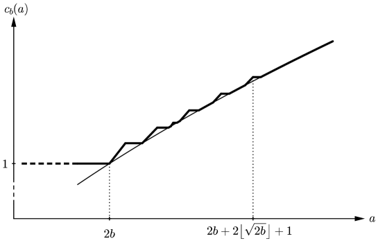
Figure 1.5. The graph of $c_{9}(a)$

The length of the affine step is $\beta_{b}-\alpha_{b}<\beta_{b}-v_{b}(1)=\frac{1}{2b(b+1)^{2}}+\frac{4}{(2b+1)^{2}}$, and hence this step becomes very small for $b$ large. The length of the $k$’th linear step is

$$\ell_{b}(k)\,:=\,v_{b}(k)-u_{b}(k)\,=\,(2b-k^{2})\,\frac{8b^{2}+k^{2}+(2+8k)b}{2b(2b+k)^{2}}.$$

For fixed $b$, the function $\ell_{b}(k)$ is strictly decreasing, with $\ell_{b}(\sqrt{2b})=0$. For fixed $k$, however, $\lim_{b\to\infty}\ell_{b}(k)=2$. More precisely, $\ell_{b}(0)$ is strictly decreasing to $2$, and $\ell_{b}(k)$ is strictly increasing to $2$ for every $k\geqslant 1$. Since the edge of the $k$’th step is at $2b+2k+1$, we see that for $b\to\infty$, an arbitrarily large (but fixed) part of the graph of $c_{b}(a)$ consists of linear steps of length almost $2$, that almost form a connected staircase (Figure 1.6).

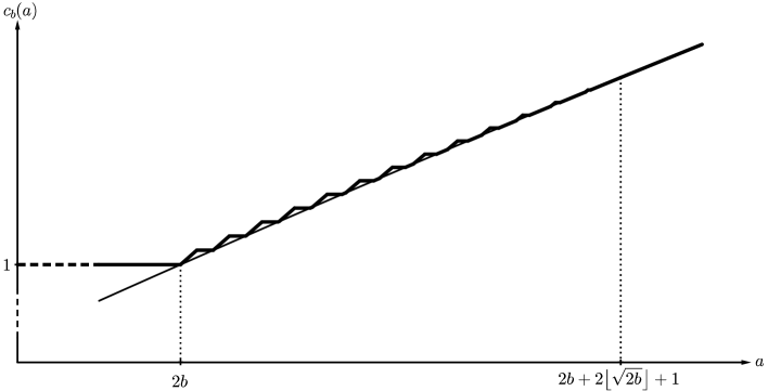
Figure 1.6. The graph of $c_{85}(a)$

We reformulate this behaviour of $c_{b}(a)$ for large $b$ in terms of a rescaled limit function: Consider the rescaled functions

$$\hat{c}_{b}(a)\,=\,2b\,c_{b}(a+2b)-2b,\qquad a\geqslant 0,$$

that are obtained from $c_{b}(a)$ by first forgetting about the horizontal line $c_{b}(a)=1$ over $[1,2b]$ that comes from the Nonsqueezing Theorem, then vertically rescaling by $2b$, and finally translating the graph by the vector $(-2b,-2b)$. Further, consider the function $c_{\infty}\colon[0,\infty)\to\mathbbm{R}$ drawn in Figure 1.7; its graph consists of infinitely many steps of width $2$ and slope $1$ that are based at the line $\frac{a}{2}$. Then

(1.3) $$\lim_{b\to\infty}\hat{c}_{b}(a)\,=\,c_{\infty}(a),\qquad a\in[0,\infty),$$

uniformly on bounded sets. Indeed, applying the same rescaling to $\sqrt{\frac{a}{2b}}$ yields $2b\sqrt{\frac{a+2b}{2b}}-2b$, which is $\frac{a}{2}+O(\frac{a^{2}}{2b})$ for $b\geqslant a$. One can also check that $\hat{c}_{b}(a)$ is increasing to $c_{\infty}(a)$ for all $a$.

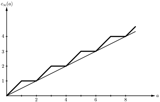
Figure 1.7. The graph of the rescaled limit function $c_{\infty}(a)$

1.3. Interpretation

Recall from the introduction that the graph of $c_{C}(a)$ has three parts: Fist the infinite Pell stairs, then one affine step, and then six more steps.

If we take $b=1$ in the above description of $c_{b}(a)$ on $[1,v_{b}(1)]$, we exactly obtain $c_{C}(a)$ on $[1,v_{1}(1)]=[1,\frac{50}{9}]$. Further, if we take $b=1$ in the description (iii) of the affine step of $c_{b}(a)$, we exactly obtain the affine step of $c_{C}(a)$ over $[\sigma^{2},6\frac{1}{8}]$. Hence $c_{b}(a)$ generalizes $c_{C}(a)$ on the first two steps and on the affine step. This is not a coincidence. Indeed, the two exceptional classes giving rise to the first two steps of the Pell stairs are the first two in the sequence (1.4) of exceptional classes $E_{n}$ giving rise to all the linear steps of $c_{b}(a)$, and the exceptional class giving rise to the affine step of $c_{C}(a)$ is the first in a sequence of exceptional classes $F_{b}$ giving rise to the affine step in $c_{b}(a)$; see § 3.

On the other hand, the remaining infinitely many steps of the Pell stairs have no counterpart for $b\geqslant 2$. Similarly, the linear steps described in (ii) of Theorem 1.1 are more regular than the affine steps on the right part of $c_{C}(a)$, none of which consists of a linear and a horizontal segment. We thus see that the first two steps and the affine step of $c_{C}(a)=c_{1}(a)$ are stable under the deformations of $b$ we consider, while the other steps are not.

By Theorem 1.1, $c_{b}(a)$ equals the volume constraint $\sqrt{\frac{a}{2b}}$ for $a\geqslant v_{b}(\lfloor\sqrt{2b}\rfloor)=2b+O(\sqrt{b})$, that is, there are no packing obstructions for the embedding problem $E(1,a)\;{\stackrel{{\scriptstyle s}}{{\hookrightarrow}}}\;P(\lambda,\lambda b)$ for $a$ sufficiently large. This is not a surprise. Indeed, this phenomenon was already observed for the embedding problems $E(1,a)\;{\stackrel{{\scriptstyle s}}{{\hookrightarrow}}}\;B^{4}(b)$ and $E(1,a)\;{\stackrel{{\scriptstyle s}}{{\hookrightarrow}}}\;C^{4}(b)$, and it fits well with previous results: It is known for many closed connected symplectic manifolds $(M,\omega)$ that there is a number $N(M,\omega)$ such that $(M,\omega)$ admits a full symplectic packing by $k$ equal balls for every $k\geqslant N(M,\omega)$ (“packing stability”, see [2, 3, 5, 6, 7, 8]). Similarly, an explicit construction implies that for any connected symplectic manifold $(M,\omega)$ of finite volume, the proportion of the volume that can be filled by a dilate of the ellipsoid $E(1,\dots,1,a)$ tends to $1$ as $a\to\infty$, see [31, § 6]: The packing obstruction tends to zero as the domain is more and more elongated.

Theorem 1 exhibits a different phenomenon: If in the problem $E(1,a)\;{\stackrel{{\scriptstyle s}}{{\hookrightarrow}}}\;P(\lambda,\lambda b)$ the target is elongated ($b\to\infty$), then the regular Pell stairs in the graph of $c_{1}(a)$ first almost disappears (only two linear steps and the affine step remain), but then for large $b$ the graph of $c_{b}(a)$ reorganizes to a staircase that asymptotically is infinite and completely regular.

1.4. Stabilization and connection with symplectic folding

Let $a,b\geqslant 1$ be real numbers. Following [13] we consider for each $N\geqslant 3$ the stabilized problem

$$c_{b}^{N}(a)\,:=\,\inf\bigl{\{}\lambda>0\mid E(1,a)\times\mathbbm{C}^{N-2}\,\;{\stackrel{{\scriptstyle s}}{{\hookrightarrow}}}\;\,P(\lambda,\lambda b)\times\mathbbm{C}^{N-2}\bigr{\}}.$$

Then $c_{b}^{N}(a)\leqslant c_{b}(a)$.

Lemma 1.3.

For every $N\geqslant 3$ and all real numbers $a,b\geqslant 1$,

$$c_{b}^{N}(a)\,\leqslant\,f_{b}(a)\,:=\,\frac{2a}{a+2b-1}.$$

Proof.

Set $\mu=\frac{a(2b-1)}{a+2b-1}$ and $\lambda=2(1-\frac{\mu}{a})$. Then $\mu+\frac{\lambda}{2}=b\lambda$. Since $b\geqslant 1$ we have $\mu\geqslant\frac{\lambda}{2}$. Note that $\frac{\lambda}{2}=1-\frac{\mu}{a}$ is the area of a $z_{2}$-disc in $E(a,1)$ over a point $z_{1}$ on the boundary of the disc $D(\mu)$ of area $\mu$. Applying Hind’s folding construction in [17, § 2] with $\mu$ (instead of $\frac{S}{S+1}$) we obtain for every $\varepsilon>0$ a symplectic embedding

$$E(1,a)\times\mathbbm{C}\,\;{\stackrel{{\scriptstyle s}}{{\hookrightarrow}}}\;\,P(\mu+\tfrac{\lambda}{2}+\varepsilon,2\,\tfrac{\lambda}{2}+\varepsilon)\times\mathbbm{C}.$$

Now recall that $\mu+\frac{\lambda}{2}=b\lambda$ and note that $\lambda=f_{b}(a)$. $\Box$

In view of the above proof, we call the graph of $f_{b}(a)$ the folding curve. Now note that

$$f_{b}(2b+2k+1)\,=\,\frac{2b+2k+1}{2b+k},\qquad k\geqslant 0.$$

For $b\in\mathbbm{N}$ this is also the value of $c_{b}$ at the edge points of the $k$th linear step. In other words, the linear steps oscillate between the volume constraint $\sqrt{\frac{a}{2b}}$ and the folding curve, see Figures 1.4 and 1.8.

Conjecture 1.4.

The edge points of the linear steps are stable, in the sense that at these points we have $c_{b}^{N}=c_{b}$ for all $N\geqslant 3$.

This conjecture is based on the main result of [13], where it is shown that the edge points of the Fibonacci stairs for the problem $E(a,1)\;{\stackrel{{\scriptstyle s}}{{\hookrightarrow}}}\;B^{4}(\lambda)$ are stable. It is likely that one can prove it by a similar method as in [13], see also the discussion at the end of the next section. A proof of Conjecture 1.4 is not the concern of the present work, but a positive answer would imply that the folding construction in the proof of Lemma 1.3 is sharp at the edge points of the linear steps.

Figure 1.8. The volume constraint, $c_{b}(a)$, and the folding curve, for $b=5$

Recall that $c_{b}(a)=1$ for $a\in[1,2b]$. As we shall see in Proposition 3.5 (ii), $c_{b}(a)=\sqrt{\frac{a}{2b}}$ for all $a\geqslant(\sqrt{2b}+1)^{2}$ and all real $b\geqslant 2$. Now notice that $f_{b}(a)\geqslant\sqrt{\frac{a}{2b}}$ if and only if $a\in\bigl{[}(\sqrt{2b}-1)^{2},(\sqrt{2b}+1)^{2}\bigr{]}$. It follows that

$$c_{b}^{N}(a)\,<\,c_{b}(a)\quad\mbox{ if }\,a\notin\bigl{[}2b-1,(\sqrt{2b}+1)^{2}\bigr{]}$$

for all $b\geqslant 2$ and $N\geqslant 3$.

We finally notice that under the rescaling yielding the limit function $c_{\infty}(a)$, we have $\hat{f}_{b}(a)=2b\,f_{b}(a+2b)-2b=\frac{2b(a+1)}{a+4b-1}$, and so

$$f_{\infty}(a)\,:=\,\lim_{b\to\infty}\hat{f}_{b}(a)\,=\,\frac{a+1}{2}.$$

This means that also the limit function $c_{\infty}$ oscillates, between the limit function $\frac{a}{2}$ of the volume constraint $\sqrt{\frac{a}{2b}}$ and the limit function $\frac{a+1}{2}$ of the folding curve.

1.5. Method

In principle, there are two methods to prove Theorem 1.1: The first method (Method 1 in § 2.2, that was used in [29, 15]) is to find the strongest obstruction for the embedding problem $E(1,a)\;{\stackrel{{\scriptstyle s}}{{\hookrightarrow}}}\;P(\lambda,\lambda b)$ coming from exceptional classes (i.e., homology classes in a certain multiple blow-up of $\operatorname{\mathbbm{C}P}^{2}$ represented by embedded $J$-holomorphic $-1$ spheres). The second method (Method 2 in § 2.2, that was first used in [8]) is a cohomological version of the first method: One associates to a hypothetical embedding $E(1,a)\;{\stackrel{{\scriptstyle s}}{{\hookrightarrow}}}\;P(\lambda,\lambda b)$ a cohomology class, and checks whether this class transforms to a “reduced vector” under Cremona transforms. While the first method is sufficient for solving the problems $E(1,a)\;{\stackrel{{\scriptstyle s}}{{\hookrightarrow}}}\;B^{4}(\lambda)$ and $E(1,a)\;{\stackrel{{\scriptstyle s}}{{\hookrightarrow}}}\;C^{4}(\lambda)$, see [29, 15], it does not lead to a proof of the entire Theorem 1.1, because the known upper bound for the number of obstructive exceptional classes tends to infinity with $b$. On the other hand, Method 2 does yield a proof of Theorem 1.1, as will become clear from our proof. We shall not follow such a puristic approach, however, but an opportunistic one, that uses both methods: Given $b$, we first write down a finite set of exceptional classes that yield embedding obstructions, namely $E_{0}=(1,0;1)$ and

(1.4) $$E_{n} := \left(n,1;1^{\times(2n+1)}\right),\quad n=b,\dots,b+\lfloor\sqrt{2b}\rfloor,$$

$$F_{b} := \left(b(b+1),b+1;b+1,b^{\times(2b+3)}\right),$$

(see § 2.2 for the notation), and then use Method 2 to show that the obstruction $f_{b}(a)$ given by these classes is complete. In other words, we use Method 1 to show $c_{b}(a)\geqslant f_{b}(a)$ and Method 2 to show $c_{b}(a)\leqslant f_{b}(a)$ (with the exception that for $a$ large and for $b=2$ and $a\in[8\frac{1}{36},9]$ we use Method 1 to show that $c_{b}(a)$ equals the volume constraint $\sqrt{\frac{a}{2b}}$).

This hybrid approach yields the shortest proof of Theorem 1.1 we know. Further, knowing a set of exceptional classes that provide all embedding obstructions is interesting for at least two reasons: First, the holomorphic spheres underlying these classes provide a geometric explanation of the graphs of the functions $c_{b}(a)$. Second, one should be able to use these holomorphic spheres to prove Conjecture 1.4; it is probably the case that one can find the needed obstructions by stretching these spheres and then “stabilizing” as in [13, 18].

1.6. Outlook

Our ultimate goal is to see the continuous film of graphs $c_{b}(a)$ for $b\geqslant 1$ real. It would be particularly interesting to understand this film for $b\in[1,2]$, or just for $b\in[1,1+{\varepsilon}]$ for some ${\varepsilon}>0$, namely to understand how the Pell stairs disappear. In [4], ECH-capacities are used to compute $c_{b}(a)$ for $b=\frac{13}{2}$ and to get an idea of this film. In accordance with Theorem 1.1, Conjecture 6.3 in [4] and further investigations we make the

Conjecture 1.5.

For any real $b\geqslant 2$ the function $c_{b}(a)$ is given by the maximum of the volume constraint $\sqrt{\frac{a}{2b}}$ and the obstructions coming from the exceptional classes $E_{n}$ and $F_{n}$ in (1.4).

The obstructions given by the exceptional classes $E_{n}$ and $F_{n}$ are readily computed, see § 3.3: While the classes $E_{n}$ again give rise to a finite staircase with linear steps, the classes $F_{n}$ give an obstruction only for $b\in(n-\frac{n}{(n+1)^{2}},n+\frac{1}{n+2})$. While our proof of Theorem 1.1 should extend to a proof of Conjecture 1.5, the analysis is more involved, since fractional parts arise, that are harder to estimate.

Our only definite result for $b$ real is that for every real $b\geqslant 2$ we have $c_{b}(a)=\sqrt{\frac{a}{2b}}$ for all $a\geqslant(\sqrt{2b}+1)^{2}$, see Proposition 3.5 (ii).

Acknowledgment. We cordially thank Dusa McDuff, who already in 2010 suggested to us to use the reduction method for analyzing the embedding problem $E(1,a)\;{\stackrel{{\scriptstyle s}}{{\hookrightarrow}}}\;C^{4}(\lambda)$.

2. Methods of proof

In this section we describe the methods we will use in the proof of Theorem 1.1. For more details we refer to the surveys [12, 20, 32] and the given references.

2.1. Translation to a ball packing problem

Fix $b\geqslant 1$. Since the function $c_{b}(a)$ is continuous in $a$, it suffices to compute $c_{b}(a)$ for $a\geqslant 1$ rational. The weight expansion $\boldsymbol{w}(a)$ of such an $a$ is the finite decreasing sequence

$$\boldsymbol{w}(a) := \bigl{(}\underbrace{1,\dots,1}_{\ell_{0}},\,\underbrace{w_{1},\dots,w_{1}}_{\ell_{1}},\,\dots,\,\underbrace{w_{N},\dots,w_{N}}_{\ell_{N}}\bigr{)}$$

$$\equiv \bigl{(}1^{\times\ell_{0}},\,w_{1}^{\times\ell_{1}},\,\dots,\,w_{N}^{\times\ell_{N}}\bigr{)}$$

such that $w_{1}=a-\ell_{0}<1$, $w_{2}=1-\ell_{1}w_{1}<w_{1}$, and so on. For example, $a=25/9$ has weight expansion $\boldsymbol{w}(a)=(1,1,\frac{7}{9},\frac{2}{9},\frac{2}{9},\frac{2}{9},\frac{1}{9},\frac{1}{9})\equiv(1^{\times 2},\frac{7}{9},\frac{2}{9}\,\!^{\times 3},\frac{1}{9}\,\!^{\times 2})$.

Write $B(\boldsymbol{w}(a))$ for the disjoint union of balls $B(1)\coprod\dots\coprod B(w_{N})$ whose weights are those appearing in $\boldsymbol{w}(a)$, with multiplicities. Based on [25] it was shown in [15, Prop. 1.4] that $E(1,a)\;{\stackrel{{\scriptstyle s}}{{\hookrightarrow}}}\;P(\lambda,\lambda b)$ if and only if

(2.2) $$B(\boldsymbol{w}(a))\coprod B(\lambda)\coprod B(\lambda b)\,\;{\stackrel{{\scriptstyle s}}{{\hookrightarrow}}}\;\,B(\lambda(b+1)),$$

cf. the moment map picture on the left of Figure 2.2.

2.2. Three translations to a combinatorial problem

In order to reformulate problem (2.2), we look at the general ball packing problem

(2.3) $$\coprod_{i=1}^{n}B(a_{i})\;{\stackrel{{\scriptstyle s}}{{\hookrightarrow}}}\;B(\mu).$$

We shall describe three combinatorial solutions of (2.3).

Denote by $X_{n}$ the $n$-fold complex blow-up of $\operatorname{\mathbbm{C}P}^{2}$, endowed by the orientation induced by the complex structure. Its homology group $H_{2}(X_{n};\mathbbm{Z})$ has the canonical basis $\{L,E_{1},\dots,E_{n}\}$, where $L=[\operatorname{\mathbbm{C}P}^{1}]$ and the $E_{i}$ are the classes of the exceptional divisors. The Poincaré duals of these classes are denoted $\ell,e_{1},\dots,e_{n}$. Let $K:=-3L+\sum_{i=1}^{n}E_{i}$ be the Poincaré dual of $-c_{1}(X_{n})$, and consider the $K$-symplectic cone ${\mathcal{C}}_{K}(X_{n})\subset H^{2}(X_{n};\mathbbm{R})$, namely the set of cohomology classes that can be represented by symplectic forms $\omega$ on $X_{n}$ that are compatible with the orientation of $X_{n}$ and have first Chern class $c_{1}(\omega)=c_{1}(X_{n})=\operatorname{PD}(-K)$. Denote by $\overline{{\mathcal{C}}_{K}}(X_{n})$ its closure in $H^{2}(X_{n};\mathbbm{R})$.

McDuff–Polterovich [28] proved that an embedding (2.3) exists if and only if

$$\mu\ell-\sum_{i=1}^{n}a_{i}e_{i}\,\in\,\overline{{\mathcal{C}}_{K}}(X_{n}).$$

We thus need to describe $\overline{{\mathcal{C}}_{K}}(X_{n})$. For this consider the set ${\mathcal{E}}_{K}(X_{n})\subset H_{2}(X_{n};\mathbbm{Z})$ of classes $E$ with $-K\cdot E=c_{1}(E)=1$, $E\cdot E=-1$ that can be represented by smoothly embedded spheres. Li–Liu [23] characterized $\overline{{\mathcal{C}}_{K}}(X_{n})$ as

(2.4) $$\overline{{\mathcal{C}}_{K}}(X_{n})\,=\,\left\{\alpha\in H^{2}(X_{n};\mathbbm{R})\mid\alpha^{2}\geqslant 0\mbox{ and }\alpha(E)\geqslant 0\mbox{ for all }E\in{\mathcal{E}}_{K}(X_{n})\right\}.$$

We thus need to describe ${\mathcal{E}}_{K}(X_{n})$. For this define for $n\geqslant 3$ the Cremona transform $\operatorname{Cr}\colon\mathbbm{R}^{1+n}\to\mathbbm{R}^{1+n}$ as the linear map taking $(x_{0};\,x_{1},\dots,x_{n})$ to

(2.5) $$\left(2x_{0}-x_{1}-x_{2}-x_{3};\,x_{0}-x_{2}-x_{3},\,x_{0}-x_{1}-x_{3},\,x_{0}-x_{1}-x_{2},\,x_{4},\,\dots,\,x_{n}\right).$$

A vector $(x_{0};\,x_{1},\dots,x_{n})$ is ordered if $x_{1}\geqslant\dots\geqslant x_{n}$. The standard Cremona move takes an ordered vector $(x_{0};\boldsymbol{x})$ to the vector obtained by ordering $\operatorname{Cr}(x_{0};\boldsymbol{x})$. More generally, a Cremona move is a Cremona transform followed by any permutation of the components of $\boldsymbol{x}$.

For later use we recall the geometric origin of $\operatorname{Cr}$ and of Cremona moves. For any non-zero vector $u$ in an inner-product space, the map $r_{u}(x)=x-2\,\frac{\langle u,x\rangle}{\langle u,u\rangle}\,u$ is the reflection about $u$, and hence an involution. Similarly, for a class $A\in H_{2}(X_{n};\mathbbm{R})$ with $A\cdot A\neq 0$ the map $r_{A}(B)=B-2\,\frac{A\cdot B}{A\cdot A}\,A$ is an involution of $H_{2}(X_{n};\mathbbm{R})$. For $|A\cdot A|\in\{1,2\}$, this map is also an automorphism of $H_{2}(X_{n};\mathbbm{Z})$. Now take the classes $A_{0}=L-E_{1}-E_{2}-E_{3}$ and $A_{ij}=E_{i}-E_{j}$ for $1\leqslant i<j\leqslant n$. Their self-intersection number is $-2$, and so for these classes,

(2.6) $$r_{A}(B)\,=\,B+(A\cdot B)\,A.$$

With respect to the basis $\{L,E_{1},\dots,E_{n}\}$ we have that $r_{A_{0}}$ is given by (2.5), that is, $r_{A_{0}}=\operatorname{Cr}\colon\mathbbm{Z}^{1+n}\to\mathbbm{Z}^{1+n}$ takes the integral vector $(d;\boldsymbol{m})=(d;m_{1},\dots,m_{n})$ to

(2.7) $$\left(2d-m_{1}-m_{2}-m_{3};\,d-m_{2}-m_{3},\,d-m_{1}-m_{3},\,d-m_{1}-m_{2},\,m_{4},\,\dots,\,m_{n}\right),$$

and $r_{A_{ij}}$ is the transposition $\tau_{ij}$ interchanging the $i$th and $j$th coordinate. These involutions of $H_{2}(X_{n};\mathbbm{Z})$ are induced by orientation preserving diffeomorphisms of $X_{n}$. This is clear for $\tau_{ij}$ (lift to $X_{n}$ an isotopy of $\operatorname{\mathbbm{C}P}^{2}$ interchanging holomorphically small discs around the $i$th and $j$th blow-up points), and it holds for all classes $A_{0},A_{ij}$ because each of them can be represented by a smoothly embedded sphere $S$, and the smooth version of the Dehn–Seidel twist along $S$, [33], is a diffeomorphism inducing (2.6), in view of the Picard–Lefschetz formula [1, p. 26]. Since the maps $\operatorname{Cr}$ and $\tau_{ij}$ preserve both the intersection product on $H_{2}(X_{n};\mathbbm{Z})$ and the class $K$, they preserve the set ${\mathcal{E}}_{K}(X_{n})$.

Based on [22, 23] it was shown in [29, Prop. 1.2.12] that a homology class $E=dL-\sum_{i=1}^{n}m_{i}E_{i}$ belongs to ${\mathcal{E}}_{K}(X_{n})$ if and only if the vector $(d;\boldsymbol{m})=(d;m_{1},\dots,m_{n})$ is equal to $(0;\,-1,0,\dots,0)$ up to a permutation of the $m_{i}$, or if $(d;\boldsymbol{m})\in\mathbbm{N}\cup(\mathbbm{N}\cup\{0\})^{n}$ satisfies the Diophantine system

(2.8) $$\sum_{i=1}^{n}m_{i}=3d-1,\qquad\sum_{i=1}^{n}m_{i}^{2}=d^{2}+1$$

and reduces to $(0;\,-1,0,\dots,0)$ under repeated standard Cremona moves. Summarizing, we find

Method 1 (Obstructive classes) An embedding (2.3) exists if and only if $\sum_{i=1}^{n}a_{i}^{2}\leqslant\mu^{2}$ and $\sum_{i=1}^{n}a_{i}\,m_{i}\leqslant\mu d$ for all vectors $(d;\boldsymbol{m})$ of non-negative integers satisfying (2.8) and reducing to $(0;-1,\,0,\,\dots,\,0)$ under repeated standard Cremona moves.

Remark 2.1.

It is shown in [25] (see also [20]) that (2.3) is also equivalent to $\sum_{i=1}^{n}a_{i}\,m_{i}\leqslant\mu d$ for all vectors $(d;\boldsymbol{m})$ of non-negative integers satisfying the Diophantine system (2.8). It follows that if we use exceptional classes only to give lower bounds for $c_{b}(a)$ (as we do in this paper), then we do not need to show that these classes reduce to $(0;\,-1,0,\dots,0)$ under repeated standard Cremona moves. We shall nevertheless perform these reductions, since they are readily done (see § 3.2) and since we wish to know explicit exceptional classes responsible for the embedding obstructions beyond the volume constraint.

In view of (2.2) we find that $E(1,a)\;{\stackrel{{\scriptstyle s}}{{\hookrightarrow}}}\;P(\lambda,\lambda b)$ if and only if $\lambda\geqslant\sqrt{\frac{a}{2b}}$ and

(2.9) $$\lambda(b+1)\,\geqslant\,\lambda\left(bm_{1}+m_{2}\right)+m_{3}\,w_{1}+\dots+m_{k+2}\,w_{k}$$

for all vectors $(d;\boldsymbol{m})$ of non-negative integers satisfying (2.8) with $n=k+2$ and reducing to $(0;-1,\,0,\,\dots,\,0)$ under repeated standard Cremona moves.

Condition (2.9) is not handy, since $\lambda$ appears on both sides. We thus better work directly in $P(\lambda,\lambda b)$ or in its compactification $S^{2}\times S^{2}$ endowed with the product symplectic form of the same volume. Let $Y_{k+1}$ be the complex blow-up of $S^{2}\times S^{2}$ in $k+1$ points. Then the classes $S_{1}=[S^{2}\times{\rm pt}]$, $S_{2}=[{\rm pt}\times S^{2}]$ and the classes $F_{1},\dots,F_{k+1}$ of the exceptional divisors form a basis of $H_{2}(Y_{k+1})$. As one can guess from the picture on the right of Figure 2.2, there exists a diffeomorphism $\psi\colon Y_{k+1}\to X_{k+2}$ such that the induced map $\psi_{*}\colon H_{2}(Y_{k+1})\to H_{2}(X_{k+2})$ is given by

$$S_{1} \mapsto L-E_{1},$$

$$S_{2} \mapsto L\phantom{-E_{1}}-E_{2},$$

$$F_{1} \mapsto L-E_{1}-E_{2},$$

$$F_{i} \mapsto \phantom{L-E_{1}-E_{2}}-E_{i+1},\quad i\geqslant 2.$$

If we write $(d,e;m_{1},\dots,m_{k+1})$ for $dS_{1}+eS_{2}-m_{1}F_{1}-\dots-m_{k+1}F_{k+1}$, we thus have

(2.10) $$\psi_{*}(d,e;\boldsymbol{m})\,=\,\left(d+e-m_{1};d-m_{1},e-m_{1},m_{2},\dots,m_{k+1}\right).$$

Given $\boldsymbol{u}\in\mathbbm{R}^{n_{1}},\boldsymbol{v}\in\mathbbm{R}^{n_{2}}$ we write $\langle\boldsymbol{u},\boldsymbol{v}\rangle=\sum_{i=1}^{\max(n_{1},n_{2})}u_{i}\,v_{i}$. In the basis $S_{1},S_{2},F_{1},\dots,F_{k+1}$, we can reformulate Method 1 as

Method 1’ (Obstructive classes) An embedding $E(1,a)\;{\stackrel{{\scriptstyle s}}{{\hookrightarrow}}}\;P(\lambda,\lambda b)$ exists if and only if $\lambda\geqslant\sqrt{\frac{a}{2b}}$ and

(2.11) $$\lambda\,\geqslant\,\frac{\langle\boldsymbol{m},\boldsymbol{w}(a)\rangle}{d+be}\,=:\,\mu_{b}(d,e;\boldsymbol{m})(a)$$

for all vectors $(d,e;\boldsymbol{m})$ of non-negative integers that satisfy the Diophantine system

(2.12) $$\sum m_{i}=2(d+e)-1,\qquad\sum m_{i}^{2}=2de+1$$

and for which $\psi_{*}(d,e;\boldsymbol{m})$ reduces to $(0;\,-1,0,\dots,0)$ under repeated standard Cremona moves.

For the detailed translation of Method 1 to Method 1’ we refer to the proof of Proposition 3.9 in [15]. As we shall see in Section 3, the obstructions to embeddings $E(1,a)\;{\stackrel{{\scriptstyle s}}{{\hookrightarrow}}}\;P(\lambda,\lambda b)$ beyond the volume (that is, the steps in the graphs $c_{b}(a)$) are all given by the following two series of exceptional classes $(d,e,\boldsymbol{m})$:

(2.13) $$E_{n} := \left(n,1;1^{\times(2n+1)}\right),$$

$$F_{n} := \left(n(n+1),n+1;n+1,n^{\times(2n+3)}\right).$$

In Method 1, the Cremona moves acted on integral homology classes $(d;\boldsymbol{m})$. The second method applies Cremona moves to real cohomology classes $\alpha$, and verifies by a finite algorithm whether $\alpha\in\overline{{\mathcal{C}}_{K}}(X_{n})$.

For convenience, we write $(\mu;a_{1},\dots,a_{n})$ instead of $\mu\ell-\sum_{i=1}^{n}a_{i}e_{i}$. Recall that the Cremona transform $\operatorname{Cr}$ on $H_{2}(X_{n};\mathbbm{Z})$ is induced by an orientation preserving diffeomorphism $\varphi$ of $X_{n}$. Since $\operatorname{Cr}=\varphi_{*}$ is an involution, the map $\varphi^{*}$ induced on cohomology $H^{2}(X_{n};\mathbbm{R})$ is also given by formula (2.5), with respect to the Poincaré dual basis $\{\ell,e_{1},\dots,e_{n}\}$, that is, $\varphi^{*}=\operatorname{Cr}\colon\mathbbm{R}^{1+n}\to\mathbbm{R}^{1+n}$ takes the vector $(\mu;a_{1},\dots,a_{n})$ to

(2.14) $$\left(2\mu-a_{1}-a_{2}-a_{3};\,\mu-a_{2}-a_{3},\,\mu-a_{1}-a_{3},\,\mu-a_{1}-a_{2},\,a_{4},\,\dots,\,a_{n}\right).$$

Call an ordered vector $(\mu;a_{1},\dots,a_{n})$ reduced if $\mu\geqslant a_{1}+a_{2}+a_{3}$. Using the characterisation (2.4) and building on [22, 23], Buse–Pinsonnault [8, §2.3] and Karshon–Kessler [21, §6.3] designed the following algorithm to decide whether an embedding (2.3) exists.

Method 2 (Reduction at a point) Let $\alpha=(\mu;a_{1},\dots,a_{n})$ be an ordered vector with $\mu\geqslant 0$ and $\alpha^{2}\geqslant 0$. The sequence obtained from applying to $\alpha$ standard Cremona moves contains a reduced vector. Let $(\hat{\mu};\,\hat{a}_{1},\dots,\hat{a}_{n})$ be the first reduced vector in this sequence. Then $\alpha\in\overline{{\mathcal{C}}_{K}}(X_{n})$ if and only if $\hat{a}_{1},\dots,\hat{a}_{n}\geqslant 0$.

We shall only need the if-part of this equivalence. In fact, we shall use a version thereof that will permit us to avoid finding the reordering after each Cremona transform:

Proposition 2.2.

Let $\alpha=(\mu;a_{1},\dots,a_{n})$ be a vector with $\mu\geqslant 0$ and $\alpha^{2}\geqslant 0$, and assume that there is a sequence $\alpha=\alpha_{0},\alpha_{1},\dots,\alpha_{m}$ of vectors such that $\alpha_{j+1}$ is obtained from $\alpha_{j}$ by a Cremona move. If $\alpha_{m}=(\hat{\mu};\,\hat{a}_{1},\dots,\hat{a}_{n})$ is reduced and $\hat{a}_{1},\dots,\hat{a}_{n}\geqslant 0$, then $\alpha\in\overline{{\mathcal{C}}_{K}}(X_{n})$.

Proof.

According to Proposition 4.9 (3) in [23], a reduced vector with non-negative coefficients belongs to $\overline{{\mathcal{C}}_{K}}(X_{n})$. Hence $\alpha_{m}\in\overline{{\mathcal{C}}_{K}}(X_{n})$. By assumption, $\alpha_{m}=(\pi\circ\operatorname{Cr})(\alpha_{m-1})$, where $\pi$ is a coordinate-permutation of $\mathbbm{R}^{n}$. Write $\pi$ as a product $\tau_{s}\circ\dots\circ\tau_{1}$ of transpositions. Since $\operatorname{Cr}$ and $\tau_{i}$ are involutions,

$$\alpha_{m-1}\,=\,\left(\operatorname{Cr}\circ\tau_{1}\circ\dots\circ\tau_{s}\right)(\alpha_{m}).$$

Recall that $\operatorname{Cr}$ and $\tau_{i}$ preserve the set ${\mathcal{E}}_{K}(X_{n})$. In view of (2.4), these maps also preserve $\overline{{\mathcal{C}}_{K}}(X_{n})$. Thus $\alpha_{m-1}\in\overline{{\mathcal{C}}_{K}}(X_{n})$. Iterating this argument yields $\alpha=\alpha_{0}\in\overline{{\mathcal{C}}_{K}}(X_{n})$. $\Box$

It turns out that for transforming a (reducible) vector to a reduced vector by Cremona moves, it is best to reorder every vector in the process. In our reduction schemes in Sections 5–8 we will usually do this, but not always, to avoid distinguishing even more cases. The point of Proposition 2.2 is that even when we do restore the order of a vector, we do not need to prove this, except for the head of the last vector: All we need to make sure is that we eventually arrive at a vector $(\hat{\mu};\hat{a}_{1},\hat{a}_{2},\hat{a}_{3},\hat{a}_{4},\dots)$ that is reduced and has $\hat{a}_{j}\geqslant 0$ for all $j$, i.e., is such that

$$\min\{\hat{a}_{1},\hat{a}_{2},\hat{a}_{3}\}\geqslant\max\{\hat{a}_{4},\dots,\hat{a}_{n}\},\quad\hat{\mu}\geqslant\hat{a}_{1}+\hat{a}_{2}+\hat{a}_{3},\quad\hat{a}_{j}\geqslant 0\mbox{ for all~{}$j$.}$$

On the other hand, we will always immediately check in each step that the new coefficients are non-negative, since otherwise we may easily forget checking a coefficient at the end.

Recall that an embedding $E(1,a)\;{\stackrel{{\scriptstyle s}}{{\hookrightarrow}}}\;P(\lambda,\lambda b)$ exists if and only if an embedding (2.2) exists. Together with Proposition 2.2 we find the following recipe.

Proposition 2.3.

An embedding $E(1,a)\;{\stackrel{{\scriptstyle s}}{{\hookrightarrow}}}\;P(\lambda,\lambda b)$ exists if there exists a finite sequence of Cremona moves that transforms the vector (4.1) to an ordered vector with non-negative entries and defect $\delta\geqslant 0$.

In our applications of this proposition we will have $\lambda\in(1,2)$. The first Cremona transform thus maps

$$\bigl{(}(b+1)\lambda;\,b\lambda,\,\lambda,\,1^{\times\lfloor a\rfloor},\,w_{1}^{\times\ell_{1}},\,\dots\bigr{)}$$

with $\delta=-1$ to the vector

$$\bigl{(}(b+1)\lambda-1;\,b\lambda-1,\,\lambda-1,\,0,\,1^{\times(\lfloor a\rfloor-1)},\,w_{1}^{\times\ell_{1}},\dots\bigr{)}$$

which reorders to

$$\bigl{(}(b+1)\lambda-1;\,b\lambda-1,\,1^{\times(\lfloor a\rfloor-1)}\parallel\lambda-1,\,w_{1}^{\times\ell_{1}},\dots\bigr{)}.$$

The action of this Cremona move on the balls

$$B(\boldsymbol{w}(a))\coprod B(\lambda)\coprod B(b\lambda)\,\;{\stackrel{{\scriptstyle s}}{{\hookrightarrow}}}\;\,B((b+1)\lambda)$$

with $B(\boldsymbol{w}(a))\;{\stackrel{{\scriptstyle s}}{{\hookrightarrow}}}\;P(\lambda,b\lambda)$ is illustrated in Figure 2.2.

Notation 2.4.

Above, the symbol $\parallel$ indicates that the terms before $\parallel$ are ordered, while the terms after $\parallel$ are possibly not ordered, and that all terms before $\parallel$ are not less than the terms after $\parallel$.

Method 3 (ECH capacities) In [19], Hutchings used his embedded contact homology to associate with every bounded starlike domain $U\subset\mathbbm{R}^{4}$ a sequence of symplectic capacities $c_{1}(U)\leqslant c_{2}(U)\leqslant\dots$. For an ellipsoid $E(a,b)$, this sequence is given by arranging the numbers of the form $ma+nb$ with $m,n\geqslant 0$ in nondecreasing order, with multiplicities. For instance,

$$\bigl{(}c_{k}(E(1,1))\bigr{)}=\bigl{(}1,1,2,2,2,3,3,3,3,4,\dots\bigr{)}.$$

McDuff showed in [27] that ECH-capacities provide a complete set of invariants for the embedding problem $E(a,b)\;{\stackrel{{\scriptstyle s}}{{\hookrightarrow}}}\;E(c,d)$:

$$E(a,b)\;{\stackrel{{\scriptstyle s}}{{\hookrightarrow}}}\;E(c,d)\quad\Longleftrightarrow\;c_{k}(E(a,b))\leqslant c_{k}(E(c,d))\;\mbox{ for all }k\geqslant 1.$$

Since the embedding problems $E(1,a)\;{\stackrel{{\scriptstyle s}}{{\hookrightarrow}}}\;E(\lambda,\lambda 2b)$ and $E(1,a)\;{\stackrel{{\scriptstyle s}}{{\hookrightarrow}}}\;P(\lambda,\lambda b)$ are equivalent, it follows that

(2.15) $$c_{b}(a)\,=\,\sup_{k\geqslant 1}\left\{\frac{c_{k}(E(1,a))}{c_{k}(E(1,2b))}\right\}.$$

It is not clear, though, how to derive from this description of $c_{b}(a)$ the graphs given in Theorem 1.1.

We say that an exceptional class $E=(d,e;\boldsymbol{m})\in{\mathcal{E}}_{K}(X_{n})$ is $b$-obstructive if there is some $a\geqslant 1$ such that the obstruction function (2.11) is larger than the volume constraint,

$$\mu_{b}(d,e;\boldsymbol{m})(a)\,>\,\sqrt{\frac{a}{2b}}.$$

According to Method 1, it suffices to find all $b$-obstructive classes: The graph of $c_{b}(a)$ is given as the supremum of the constraints of the $b$-obstructive classes and of the volume constraint. Since exceptional classes are represented by holomorphic spheres, this method gives insight into the nature of the obstruction to a full embedding. It is also useful for guessing the graph of $c_{b}(a)$, by first guessing a relevant set of $b$-obstructive classes (see Section 3). On the other hand, it is sometimes hard to find all $b$-obstructive classes for a point $a$. Method 2 is very efficient at a given point $a$, at least if one has an idea what $c_{b}(a)$ should be. However, the reduction scheme often depends rather subtly on the point $a$, see Sections 5–8. The reduction method is thus quite “local in $a$”. While it is usually impossible to compute $c_{b}(a)$ by Method 3 (see however [4, 14]), this method is very useful for guessing the graph of $c_{b}(a)$, since using (2.15) and a computer one gets good lower bounds for $c_{b}(a)$.

Accordingly, we have found Theorem 1.1 as follows. We first found the exceptional classes $E_{n}$, $F_{n}$ in (2.13), then used ECH-capacities to convince ourselves that there are no further constraints besides the volume, and then proved this by the reduction method. This seems to be a convenient procedure for solving symplectic embedding problems for which ECH-capacities are known to form a complete set of invariants, such as those studied in [11].

3. Applications of Method 1

Fix a real number $b\geqslant 1$. As in (2.11) we associate with every solution $(d,e;\boldsymbol{m})$ of the Diophantine system (2.12) the obstruction function

(3.1) $$\mu_{b}(d,e;\boldsymbol{m})(a)\,=\,\frac{\langle\boldsymbol{m},\boldsymbol{w}(a)\rangle}{d+be}$$

where as before $\boldsymbol{w}(a)$ is the weight expansion of $a\geqslant 1$. Further, define the error vector ${\varepsilon}:={\varepsilon}(a)$ by

$$\boldsymbol{m}\,=\,\frac{d+be}{\sqrt{2ba}}\,\boldsymbol{w}(a)+{\varepsilon}.$$

(Here, we add zeros to $\boldsymbol{m}$ or $\boldsymbol{w}(a)$ if they do not have the same length.)

3.1. Recollections

The following proposition generalizes Lemma 4.8 in [15].

Proposition 3.1.

Fix a real number $b\geqslant 1$. Given a non-negative solution $(d,e;\boldsymbol{m})$ of (2.12) and $a\geqslant 1$, we have

• $\mu_{b}(d,e;\boldsymbol{m})(a)\,\leq\,\frac{\sqrt{2de+1}\sqrt{a}}{d+be}$;

• $\mu_{b}(d,e;\boldsymbol{m})(a)>\sqrt{\frac{a}{2b}}\;\;\Longleftrightarrow\;\;\langle{\varepsilon},\boldsymbol{w}(a)\rangle>0$;

• If $\mu_{b}(d,e;\boldsymbol{m})(a)>\sqrt{\frac{a}{2b}}$, then $d=be+h$ with $|h|<\sqrt{2b}$, and $\langle{\varepsilon},{\varepsilon}\rangle=\sum{\varepsilon}_{i}^{2}<1-\frac{h^{2}}{2b}$.

Proof.

By the Cauchy–Schwarz inequality and since $\sum w_{i}^{2}=a$,

$$(d+be)\,\mu_{b}(d,e;\boldsymbol{m})(a)\,=\,\langle\boldsymbol{m},\boldsymbol{w}(a)\rangle\,\leq\,\|\boldsymbol{m}\|\|\boldsymbol{w}(a)\|\,=\,\sqrt{2de+1}\sqrt{a},$$

proving (i). Assertion (ii) is immediate. To prove (iii), we compute

$$2(be+h)e+1\,=\,2de+1\,=\,\langle\boldsymbol{m},\boldsymbol{m}\rangle = \bigg{\langle}\frac{2be+h}{\sqrt{2ba}}\,\boldsymbol{w}(a)+{\varepsilon},\frac{2be+h}{\sqrt{2ba}}\,\boldsymbol{w}(a)+{\varepsilon}\bigg{\rangle}$$

$$= \frac{(2be+h)^{2}}{2ba}\,a+2\,\frac{2be+h}{\sqrt{2ba}}\langle\boldsymbol{w}(a),{\varepsilon}\rangle+\langle{\varepsilon},{\varepsilon}\rangle.$$

The first of the three summands is $2be^{2}+2eh+\frac{h^{2}}{2b}$, and so

$$1\,=\,\frac{h^{2}}{2b}+2\frac{2be+h}{\sqrt{2ba}}\langle\boldsymbol{w}(a),{\varepsilon}\rangle+\langle{\varepsilon},{\varepsilon}\rangle.$$

Hence, if $\mu_{b}(d,e;\boldsymbol{m})(a)>\sqrt{\frac{a}{2b}}$, then, by (ii), $\langle\boldsymbol{w}(a),{\varepsilon}\rangle>0$, whence $0\leqslant\langle{\varepsilon},{\varepsilon}\rangle<1-\frac{h^{2}}{2b}$. This also shows that $|h|<\sqrt{2b}$. $\Box$

3.2. Two sequences of exceptional classes, and their constraints

In our analysis of the functions $c_{b}(a)$, two sequences of exceptional homology classes will play a role. For each $n\in\mathbbm{N}$ we define the classes

$$E_{n} := \left(n,1;1^{\times(2n+1)}\right),$$

$$F_{n} := \left(n(n+1),n+1;n+1,n^{\times(2n+3)}\right).$$

Notice that $E_{n}$ is a perfect class at $a=2n+1$, in the sense that $\boldsymbol{m}$ is a multiple of $\boldsymbol{w}(a)$. Similarly, $F_{n}$ is nearly perfect at $a=2n+4$. While the constraints of the classes $E_{b},E_{b+1},\dots,E_{b+\lfloor\sqrt{2b}\rfloor}$ will give the $\lceil\sqrt{2b}\rceil$ linear steps in the graph of $c_{b}(a)$ centred at $2b+2k+1$, the constraint of $F_{b}$ will give the affine step of $c_{b}(a)$ centred at $2b+4$.

Lemma 3.2.

The classes $E_{n}$ and $F_{n}$ satisfy the Diophantine system (2.12), and their image under $\psi_{*}$ reduces to $(0;\,-1,0,\dots,0)$ under repeated standard Cremona moves.

Proof.

One readily checks that the classes $E_{n}$ and $F_{n}$ satisfy the Diophantine system (2.12).

For the sequel it is useful to rewrite the Cremona transform $\operatorname{Cr}$ as follows: Define the defect of a vector $(d;\boldsymbol{m})=(d;m_{1},\dots,m_{k})$ by $\delta:=d-m_{1}-m_{2}-m_{3}$. Then (2.7) can be written as

$$\operatorname{Cr}(d;\boldsymbol{m})\,=\,\left(d+\delta;\,m_{1}+\delta,\,m_{2}+\delta,\,m_{3}+\delta,\,m_{4},\,\dots,\,m_{k}\right).$$

The isomorphism $\psi_{*}$ from (2.10) maps $E_{n}=(n,1;1^{\times(2n+1)})$ to the class $(n;n-1,1^{\times 2n})$, which under one standard Cremona move is mapped to $(n-1;n-2,1^{\times 2(n-1)})$, and hence under $n$ such moves to $(0;-1)$. Next, $\psi_{*}$ maps $F_{1}$ to the class $(2;1^{\times 5})$, which reduces to $(0;-1)$ under two standard Cremona moves, Further, for $n\geqslant 2$,

$$\psi_{*}(F_{n})\,=\,\left(n^{2}+n;n^{2}-1,n^{\times(2n+3)}\right).$$

Under $n$ standard Cremona moves with $\delta=-n+1$ this vector reduces to

$$\left(2n;n^{\times 3},n-1,1^{\times 2n}\right).$$

Applying one more standard Cremona move with $\delta=-n$ yields the vector $(n;n-1,1^{\times 2n})$, which reduces in $n$ steps to $(0;-1)$, as we have seen above. $\Box$

We next compute the constraints given by the classes $E_{n}$ and $F_{n}$. In view of definition (3.1) and the definition of these classes,

$$\mu_{b}(E_{b+k})(a)\,=\,\frac{\langle 1^{\times(2b+2k+1)},\boldsymbol{w}(a)\rangle}{2b+k}\quad\mbox{ and }\quad\mu_{b}(F_{b})(a)\,=\,\frac{\langle\bigl{(}b+1,b^{\times(2b+3)}\bigr{)},\boldsymbol{w}(a)\rangle}{2b(b+1)}.$$

From this we readily find

Lemma 3.3.

Fix an integer $b\geqslant 2$.

• For $k\in\bigl{\{}0,1,2,\dots,\lfloor\sqrt{2b}\rfloor\bigr{\}}$,

  $$\mu_{b}(E_{b+k})(a)\,=\,\left\{\begin{array}[]{cl}\frac{a}{2b+k}&\mbox{if }\;a\in[2b+2k,2b+2k+1],\\[1.99997pt] \frac{2b+2k+1}{2b+k}&\mbox{if }\;a\geqslant 2b+2k+1.\end{array}\right.$$

• $$\mu_{b}(F_{b})(a)\,=\,\left\{\begin{array}[]{cl}\frac{ba+1}{2b(b+1)}&\mbox{if }\;a\in[2b+3,2b+4],\\[1.99997pt] 1+\frac{2b+1}{2b(b+1)}&\mbox{if }\;a\geqslant 2b+4.\end{array}\right.$$

We in particular see that the class $E_{b+k}$ gives rise to the linear step over $I_{b}(k)$ and $F_{b}$ gives rise to the affine step over $[\alpha_{b},\beta_{b}]$.

3.3. The constraints of $E_{n},F_{n}$ for real $b\geqslant 2$

In this paragraph we compute the obstructions to the problem $E(1,a)\to P(\lambda,\lambda b)$ given by the exceptional classes $E_{n}$ and $F_{n}$ for all real $b\geqslant 2$. This is not used in the proof of Theorem 1.1, but supports Conjecture 1.5.

Let $b\geqslant 2$ be a real number. Recall that for $a\geqslant 1$ every exceptional class $E=(d,e;\boldsymbol{m})$ yields the constraint

$$\mu_{b}(E)(a)\,=\,\frac{\langle\boldsymbol{m},\boldsymbol{w}(a)\rangle}{d+be}.$$

For $E_{0}=(1,0;1)$ we have

(3.2) $$\mu_{b}(E_{0})(a)\,=\,1,$$

and for $E_{n}=(n,1;1^{\times(2n+1)})$ with $n\geqslant 1$ we have

$$\mu_{b}(E_{n})(a)\,=\,\left\{\begin{array}[]{cl}\frac{a}{n+b}&\mbox{if }\;a\in[2n,2n+1],\\[1.99997pt] \frac{2n+1}{n+b}&\mbox{if }\;a\geqslant 2n+1.\end{array}\right.$$

The class $E_{n}$ is $b$-obstructive on $[2n,\infty)$ only if $\frac{2n+1}{n+b}>\sqrt{\frac{2n+1}{2b}}$, and in view of (3.2) we can also assume that $\frac{2n+1}{n+b}>1$, or, $n>b-1$. The relevant values of $n$ are thus

$$n\,\in\,\bigl{\{}\lfloor b\rfloor,\dots,\lfloor b+\sqrt{2b}\rfloor\bigr{\}}$$

where $\lfloor b\rfloor$ is the largest integer not greater than $b$. The constraint $1$ of $E_{0}$ meets the first linear step, given by $E_{\lfloor b\rfloor}$, at $a=b+\lfloor b\rfloor$, and is thus strictly above $\sqrt{\frac{a}{2b}}$ if $b\notin\mathbbm{N}$. For $n\geqslant\lfloor b\rfloor$ the step of $E_{n}$ meets the step of $E_{n+1}$ at $a=\frac{(2n+1)(n+b+1)}{n+b}$, which is $\geqslant\sqrt{\frac{a}{2b}}$ if and only if $b-n\geqslant(b-n)^{2}$. The step of $E_{\lfloor b\rfloor}$ thus meets the one of $E_{\lfloor b\rfloor+1}$ above the volume constraint, with equality if and only if $b\in\mathbbm{N}$, and all other linear steps are strictly disjoint.

Next, let ${\mathbf{b}}$ be the “integer closest to $b$”, namely $b={\mathbf{b}}+\varepsilon$ with $\varepsilon\in(-\frac{1}{2},\frac{1}{2}]$. Then

$$\mu_{b}(F_{\mathbf{b}})(a)\,=\,\left\{\begin{array}[]{cl}\frac{{\mathbf{b}}a+1}{({\mathbf{b}}+b)({\mathbf{b}}+1)}&\mbox{if }\;a\in[2{\mathbf{b}}+3,2{\mathbf{b}}+4],\\[3.00003pt] \frac{2{\mathbf{b}}^{2}+4{\mathbf{b}}+1}{({\mathbf{b}}+b)({\mathbf{b}}+1)}&\mbox{if }\;a\geqslant 2{\mathbf{b}}+4.\end{array}\right.$$

But notice that this constraint is stronger than $\sqrt{\frac{a}{2b}}$ only if

$$\mu_{b}(F_{\mathbf{b}})(2{\mathbf{b}}+4)\,=\,\frac{2{\mathbf{b}}^{2}+4{\mathbf{b}}+1}{(2{\mathbf{b}}+\varepsilon)({\mathbf{b}}+1)}\,>\,\sqrt{\frac{{\mathbf{b}}+2}{{\mathbf{b}}+\varepsilon}}$$

or, equivalently, $\varepsilon\in\bigl{(}-\frac{{\mathbf{b}}}{({\mathbf{b}}+1)^{2}},\frac{1}{{\mathbf{b}}+2}\bigr{)}$. One readily checks that the affine step defined by $\mu_{b}(F_{\mathbf{b}})$ is strictly disjoint from the two neighbouring linear steps given by $E_{{\mathbf{b}}+1}$ and $E_{{\mathbf{b}}+2}$.

For $a\geqslant 1$ and $b\geqslant 2$ let $d_{b}(a)$ be the maximum of the volume constraint $\sqrt{\frac{a}{2b}}$ and the obstructions $\mu_{b}(E_{n})(a)$ and $\mu_{b}(F_{{\mathbf{b}}})$ discussed above. Then $d_{b}(a)\geqslant c_{b}(a)$ of course, and Conjecture 1.5 claims that $d_{b}(a)=c_{b}(a)$ for all real $b\geqslant 2$.

3.4. The value of $c_{b}$ at $2b+2+\frac{1}{2b}$

Set $a_{b}:=2b+2+\frac{1}{2b}$. We will show in § 4.2 by the reduction method that $c_{b}(a_{b})=\frac{2b+1}{2b}$. (Notice that this value equals the volume constraint $\sqrt{\frac{a_{b}}{2b}}$.) Here we show this by using positivity of intersection with the class

$$G_{b}\,:=\,\left(b(2b+1),2b+1;(2b)^{\times(2b+2)},1^{\times(2b+1)}\right),\quad b\in\mathbbm{N}.$$

The $\boldsymbol{m}$ of $G_{b}$ is obtained from $2b\,\boldsymbol{w}(a_{b})$ by adding one $1$, whence $G_{b}$ is nearly perfect at $a_{b}$. One readily checks that $G_{b}$ satisfies the Diophantine system (2.12) and that its image under $\psi_{*}$ reduces to $(0;\,-1,0,\dots,0)$ under repeated standard Cremona moves. Hence $G_{b}$ is an exceptional class. Its obstruction at $a_{b}$ is

$$\mu_{b}(G_{b})(2b+2+\tfrac{1}{2b})\,=\,\frac{2b(2b+2)+1}{2b(2b+1)}\,=\,\frac{2b+1}{2b}.$$

Write $G_{b}=\bigl{(}b(2b+1),2b+1;\boldsymbol{m}_{b},1\bigr{)}$ with $\boldsymbol{m}_{b}:=\bigl{(}(2b)^{\times(2b+2)},1^{\times 2b}\bigr{)}=2b\,\boldsymbol{w}(a_{b})$. Recall that exceptional classes are represented by embedded $J$-holomorphic spheres, whence by positivity of intersection $E\cdot E^{\prime}\geqslant 0$ for any two different exceptional classes $E\neq E^{\prime}$. Applying this to $G_{b}$ and any different exceptional class $(d,e;\boldsymbol{m})$, we obtain

$$(be+d)(2b+1)\,=\,b(2b+1)e+(2b+1)d\,\geqslant\,\langle\boldsymbol{m},(\boldsymbol{m}_{b},1)\rangle\,\geqslant\,\langle\boldsymbol{m},\boldsymbol{m}_{b}\rangle\,=\,2b\langle\boldsymbol{m},\boldsymbol{w}(a_{b})\rangle.$$

Hence

$$\mu_{b}(d,e;\boldsymbol{m})(a_{b})\,=\,\frac{\langle\boldsymbol{m},\boldsymbol{w}(a_{b})\rangle}{be+d}\,\leq\,\frac{2b+1}{2b},$$

as we wished to show. $\Box$

Remarks 3.4.

(i) The classes $E_{1}$, $E_{2}$ also give rise to the first two steps of $c_{C}(a)=c_{1}(a)$, and the class $F_{1}$ gives rise to the affine step of $c_{C}(a)$, see [15]. This is the “holomorphic reason” why the first two steps of the Pell stairs and the affine step of $c_{C}(a)$ survive to all functions $c_{b}(a)$, $b\geqslant 2$. On the other hand, none of the classes $E_{n}$ with $n\geqslant 3$ and $F_{n}$ with $n\geqslant 2$ is obstructive for the problem $E(1,a)\;{\stackrel{{\scriptstyle s}}{{\hookrightarrow}}}\;C^{4}(\lambda)$, and none of the classes giving rise to the other steps of the Pell stairs, nor any of the classes giving rise to the six exceptional steps of $c_{C}(a)$ gives an obstruction for the problems $E(1,a)\;{\stackrel{{\scriptstyle s}}{{\hookrightarrow}}}\;P(\lambda,\lambda b)$ with $b\geqslant 2$.

Similarly, $G_{1}$ is the first of the sequence of exceptional classes $E(\alpha_{n})$ in [15] that imply via positivity of intersection that at the foot points of the Pell stairs there is no embedding obstruction beyond the volume constraint.

(ii) We do not know all all $b$-obstructive classes. However, using positivity of intersection and the analogues of Lemmata 3.8 and 3.11 we checked that $\mu_{b}(E)(2b+2k+1)<\frac{2b+2k+1}{2b+k}$ for any exceptional class $E\neq E_{b+k}$, and that $\mu_{b}(E)(2b+4)\leqslant\sqrt{\frac{2b+4}{2b}}$ for any exceptional class $E\neq F_{b}$, that is, $F_{b}$ is the only $b$-obstructive class at $2b+4$. For $F_{2}$ this is carried out in Lemma 3.10.

3.5. $c_{b}(a)$ for $a$ large

For $b\in\mathbbm{N}_{\geqslant 2}$ we abbreviate

$$v_{b}^{+}\,:=\,v_{b}(\lfloor\sqrt{2b}\rfloor)\,=\,2b\left(\frac{2b+2\lfloor\sqrt{2b}\rfloor+1}{2b+\lfloor\sqrt{2b}\rfloor}\right)^{2}.$$

Assertion (ii) of the following proposition improves Theorem 1.1 of [4].

Proposition 3.5.

(i) For every $b\in\mathbbm{N}_{\geqslant 2}$,

$$c_{b}(a)\,=\,\left\{\begin{array}[]{cl}\frac{2b+2\lfloor\sqrt{2b}\rfloor+1}{2b+\lfloor\sqrt{2b}\rfloor}&\mbox{if }\;a\in\bigl{[}2b+2\lfloor\sqrt{2b}\rfloor+1,v_{b}^{+}\bigr{]},\\[1.99997pt] \sqrt{\frac{a}{2b}}&\mbox{if }\;a\geqslant v_{b}^{+}.\end{array}\right.$$

(ii) For every real $b\geqslant 2$ we have $c_{b}(a)=\sqrt{\frac{a}{2b}}$ for all $a\geqslant(\sqrt{2b}+1)^{2}$.

Notice that the length of the interval $\bigl{[}2b+2\lfloor\sqrt{2b}\rfloor+1,v_{b}^{+}\bigr{]}$ in (i) is

$$\frac{\bigl{(}2b+2\lfloor\sqrt{2b}\rfloor+1\bigr{)}\bigl{(}2b-\lfloor\sqrt{2b}\rfloor^{2}\bigl{)}}{(2b+\lfloor\sqrt{2b}\rfloor)^{2}}$$

and hence positive if and only if $\lfloor\sqrt{2b}\rfloor<\sqrt{2b}$, i.e., $2b$ is not a perfect square.

Proof.

Assume that $(d,e;\boldsymbol{m})$ is a non-negative solution of (2.12). If $e=0$, then $(d,e;\boldsymbol{m})=(1,0;1)$, and so $\mu_{b}(d,e;\boldsymbol{m})(a)=1$ is smaller than the values of $c_{b}(a)$ claimed in (i) and (ii). We can thus assume that $e\geqslant 1$.

Suppose that $\mu_{b}(d,e;\boldsymbol{m})(a)>\sqrt{\frac{a}{2b}}$ for some $a\geqslant 1$. Then, by Proposition 3.1 (iii), $d<be+\sqrt{2b}$. We estimate

(3.3) $$\mu_{b}(d,e;\boldsymbol{m})(a)\,=\,\frac{\langle\boldsymbol{m},\boldsymbol{w}(a)\rangle}{be+d}\,\leq\,\frac{\sum m_{i}}{be+d}\,=\,\frac{2(d+e)-1}{be+d}\,=:\,f_{b,e}(d).$$

The function $d\mapsto f_{b,e}(d)$ is increasing. We can thus further estimate

(3.4) $$\mu_{b}(d,e;\boldsymbol{m})(a)\,\leqslant\,f_{b,e}(be+\sqrt{2b})\,=\,\frac{2\bigl{(}be+\sqrt{2b}+e\bigr{)}-1}{2be+\sqrt{2b}}\,=:\,L(b,e).$$

Claim 1. $\frac{\partial}{\partial e}L(b,e)\leqslant 0$.

Proof.

We compute

$$\frac{\partial}{\partial e}L(b,e)\,=\,\frac{2(b+1)\bigl{(}2be+\sqrt{2b}\bigr{)}-2b\bigl{(}2(be+\sqrt{2b}+e)-1\bigr{)}}{(2be+\sqrt{2b})^{2}},$$

which is $\leqslant 0$ if and only if the nominator is $\leqslant 0$. Expanding the nominator, we see that this holds if and only if $b+\sqrt{2b}\leqslant b\sqrt{2b}$, which holds true because $b\geqslant 2$. $\Box$

Proof of (ii): Assume that $(d,e;\boldsymbol{m})$ is an exceptional class with $e\geqslant 1$ and $\mu_{b}(d,e;\boldsymbol{m})(a)>\sqrt{\frac{a}{2b}}$ for some $a\geqslant(\sqrt{2b}+1)^{2}$. By (3.4) and Claim 1,

$$\mu_{b}(d,e;\boldsymbol{m})(a)\,\leqslant\,L(b,e)\,\leqslant\ L(b,1)\,=\,\frac{\sqrt{2b}+1}{\sqrt{2b}}\,\leqslant\,\sqrt{\frac{a}{2b}},$$

a contradiction.

Proof of (i): Assume from now on that $b\in\mathbbm{N}_{\geqslant 2}$. If $e=1$, then (2.12) becomes

$$\sum m_{i}\,=\,\sum m_{i}^{2}\,=\,2d+1$$

and so $(d,e;\boldsymbol{m})$ is the exceptional class $E_{d}=(d,1;1^{\times(2d+1)})$. Recall that on $[2d,2d+2]$ the obstruction function $\mu_{b}(E_{d})(a)=\frac{\langle\boldsymbol{w}(a),1^{\times(2d+1)}\rangle}{b+d}$ gives a linear step with edge at $2d+1$. If $\lfloor\sqrt{2b}\rfloor<\sqrt{2b}$, then the largest $k$ for which $E_{b+k}$ yields a constraint strictly stronger than the volume is $k=\lfloor\sqrt{2b}\rfloor$, because $\frac{2b+2k+1}{2b+k}>\sqrt{\frac{2b+2k+1}{2b}}$ if and only if $2b>k^{2}$.

We are left with showing that for $e\geqslant 2$ we have $\mu_{b}(d,e;\boldsymbol{m})(a)\leqslant\sqrt{\frac{a}{2b}}$ for all solutions $(d,e;\boldsymbol{m})$ of (2.12) and all $a\geqslant v_{b}^{+}$. Assume first that $e\geqslant 3$. Then (3.4) and Claim 1 yield

$$\mu_{b}(d,e;\boldsymbol{m})(a)\,\leqslant\,L(b,e)\,\leqslant\,L(b,3).$$

Claim 2. $L(b,3)\leqslant\sqrt{\frac{a}{2b}}$ for all $b\in\mathbbm{N}_{\geqslant 2}$ and $a\geqslant v_{b}^{+}$.

Proof.

It suffices to prove the claim for $a=v_{b}^{+}$. We have

$$L(b,3)-1\,=\,\frac{\sqrt{2b}+5}{6b+\sqrt{2b}}\quad\mbox{ and }\quad\sqrt{\frac{v_{b}^{+}}{2b}}-1\,=\,\frac{\lfloor\sqrt{2b}\rfloor+1}{2b+\lfloor\sqrt{2b}\rfloor}.$$

For $b\in\{2,3,4\}$ the inequality $\frac{\lfloor\sqrt{2b}\rfloor+1}{2b+\lfloor\sqrt{2b}\rfloor}\geqslant\frac{\sqrt{2b}+5}{6b+\sqrt{2b}}$ is readily verified. For $b\geqslant 5$ we use that $x\mapsto\frac{x+1}{2b+x}$ is increasing, and estimate

$$\sqrt{\frac{v_{b}^{+}}{2b}}-L(b,3)\,\geqslant\,\frac{(\sqrt{2b}-1)+1}{2b+(\sqrt{2b}-1)}-\frac{\sqrt{2b}+5}{6b+\sqrt{2b}}.$$

The right hand side multiplied with the product of the denominators equals $f(b):=4b\sqrt{2b}-10\>\!b-4\sqrt{2b}+5$. Since $b\,f^{\prime}(b)=6b\sqrt{2b}-2\sqrt{2b}-10\>\!b\geqslant 0$ for $b\geqslant 2$ and since $f(5)>0$, the claim follows. $\Box$

Assume now that $e=2$. We first treat the case $b\geqslant 5$. In view of (3.4) it suffices to show that $L(b,2)\leqslant\sqrt{\frac{v_{b}^{+}}{2b}}$, or

$$\frac{\sqrt{2b}+3}{4b+\sqrt{2b}}\,\leqslant\,\frac{\lfloor\sqrt{2b}\rfloor+1}{2b+\lfloor\sqrt{2b}\rfloor}.$$

This inequality is readily verified for $b=5$. For $b\geqslant 6$ the stronger inequality

$$\frac{\sqrt{2b}+3}{4b+\sqrt{2b}}\,\leqslant\,\frac{(\sqrt{2b}-1)+1}{2b+(\sqrt{2b}-1)}$$

holds true. Indeed, this inequality is equivalent to $g(b):=2b\sqrt{2b}-6b-2\sqrt{2b}+3\geqslant 0$, which holds true since $b\,g^{\prime}(b)=3b\sqrt{2b}-\sqrt{2b}-6b\geqslant 0$ for $b\geqslant 6$ and $g(6)\geqslant 0$.

Assume now that $b\in\{2,3,4\}$. Then $\sqrt{\frac{v_{b}^{+}}{2b}}=1+\frac{3}{2b+2}$. Using (3.3) this time with $d\leqslant\lfloor be+\sqrt{2b}\rfloor$ we find

$$\mu_{b}(d,2;\boldsymbol{m})(a)\,\leqslant\,f_{b,2}(\lfloor 2b+\sqrt{2b}\rfloor)\,=\,\frac{2\lfloor 2b+\sqrt{2b}\rfloor+3}{2b+\lfloor 2b+\sqrt{2b}\rfloor}.$$

For $b\in\{2,3,4\}$ the right hand side is $\leqslant 1+\frac{3}{2b+2}$. Proposition 3.5 is proven. $\Box$

3.6. The interval $[8\frac{1}{36},9]$ for $b=2$

Proposition 3.6.

$c_{2}(a)=\frac{\sqrt{a}}{2}$ for $a\in[8\frac{1}{36},9]$.

Proof.

The arguments in this section are close to those in [29, § 5.3] and [15, § 7.3]. In fact, the last step of $c_{B}(a)$ and of $c_{2}(a)$ both end at $8\frac{1}{36}$ and are given by the class $F_{2}$. There are some differences, however, and so we give a complete exposition for the convenience of the reader.

Fix a rational number $a=\frac{p}{q}\in(8,9)$, with $\frac{p}{q}$ in reduced form, with weight expansion

(3.5) $$\bigl{(}1^{\times\ell_{0}},\,w_{1}^{\times\ell_{1}},\,\dots,\,w_{N}^{\times\ell_{N}}\bigr{)}.$$

Then $w_{N}=\frac{1}{q}$ and $\sum_{j=0}^{N}\ell_{j}w_{j}=a+1-\frac{1}{q}$ by Lemma 1.2.6 of [29]. Set $M:=\ell(a):=\sum_{j=0}^{N}\ell_{j}$ and $L=\sum_{j=1}^{N}\ell_{j}=\ell(a)-8$. Then $q\geqslant L$ by Sublemma 5.1.1 of [29].

For $b=2$ the error vector $\varepsilon$ of an exceptional class $(d,e;\boldsymbol{m})$ at $a$ is

(3.6) $$\boldsymbol{m}\,=\,\frac{d+2e}{2\sqrt{a}}\,\boldsymbol{w}(a)+\varepsilon.$$

Define the partial error sums

$$\sigma\,:=\,\sum_{i=\ell_{0}+1}^{M}\varepsilon_{i}^{2}\quad\mbox{and}\quad\sigma^{\prime}\,:=\,\sum_{i=\ell_{0}+1}^{M-\ell_{N}}\varepsilon_{i}^{2}\,\leqslant\,\sigma.$$

Recall from Proposition 3.1 (iii) that for an obstructive class $(d,e;\boldsymbol{m})$ we have $d=2e+h$ with $h\in\{-1,0,1\}$, and $\sigma<1$ if $h=0$ and $\sigma<\frac{3}{4}$ if $|h|=1$. For the function

$$y(a)\,:=\,a-3\sqrt{a}+1$$

we have $y(\tfrac{p}{q})>\frac{1}{q}$ for all $\tfrac{p}{q}\in(8,9)$. Write $\ell(\boldsymbol{m})$ for the number of positive entries in $\boldsymbol{m}$.

Lemma 3.7.

Let $(d,e;\boldsymbol{m})$ be an exceptional class such that there exists $a=\frac{p}{q}\in(8,9)$ with $\ell(a)=\ell(\boldsymbol{m})$ and $\mu_{2}(d,e;\boldsymbol{m})(a)>\tfrac{\sqrt{a}}{2}$. Set $v_{M}:=\frac{d+2e}{2q\sqrt{a}}$. Then

• $\left|\sum\varepsilon_{i}\right|\leqslant\sqrt{\sigma L}$.

• If $v_{M}<1$, then $\left|\sum\varepsilon_{i}\right|\leqslant\sqrt{\sigma^{\prime}L}$.

• If $v_{M}\leqslant\frac{1}{2}$, then $v_{M}>\frac{1}{3}$ and $\sigma^{\prime}\leqslant\frac{1}{2}$. If $v_{M}\leqslant\frac{2}{3}$, then $\sigma^{\prime}\leqslant\frac{7}{9}$.

• With $\delta:=y(a)-\frac{1}{q}$ we have

  $$4e+h\,\leqslant\,\tfrac{2\sqrt{a}}{\delta}\left(\sqrt{\sigma q}-(1-\tfrac{h}{2})\right)\,\leqslant\,\tfrac{2\sqrt{a}}{\delta}\left(\tfrac{\sigma}{\delta v_{M}}-(1-\tfrac{h}{2})\right).$$

  If $v_{M}<1$, then $\sigma$ can be replaced by $\sigma^{\prime}$.

Proof.

The proofs of (i), (ii) and (iii) are as for Lemma 5.1.2 in [29]. To prove (iv) we compute

$$-\sum_{i=1}^{M}\varepsilon_{i}\,=\,\tfrac{d+2e}{2\sqrt{a}}\sum_{j=0}^{N}\ell_{j}w_{j}-\sum_{i=1}^{M}m_{i} = \tfrac{d+2e}{2\sqrt{a}}\bigl{(}a+1-\tfrac{1}{q}\bigr{)}-(2d+2e-1)$$

$$= \tfrac{4e+h}{2\sqrt{a}}\bigl{(}a+1-\tfrac{1}{q}\bigr{)}-(6e+2h-1)$$

$$= \tfrac{4e+h}{2\sqrt{a}}\bigl{(}y(a)-\tfrac{1}{q}\bigr{)}+\bigl{(}1-\tfrac{h}{2}\bigr{)},$$

where we have used (3.6) and (2.12). Then, using $q\geqslant L$ and (i), we find

$$\sqrt{\sigma q}\,\geqslant\ \sqrt{\sigma L}\,\geqslant\,\tfrac{4e+h}{2\sqrt{a}}\>\!\bigl{(}y(a)-\tfrac{1}{q}\bigr{)}+(1-\tfrac{h}{2})\,=\,\tfrac{4e+h}{2\sqrt{a}}\>\!\delta+(1-\tfrac{h}{2})\,>\,\delta\>\!v_{M}\>\!q.$$

Thus $\sqrt{q}<\frac{\sqrt{\sigma}}{\delta\>\!v_{M}}$, and so

$$4e+h\,\leqslant\,\tfrac{2\sqrt{a}}{\delta}\bigl{(}\sqrt{\sigma q}-(1-\tfrac{h}{2})\bigr{)}\,<\,\tfrac{2\sqrt{a}}{\delta}\bigl{(}\tfrac{\sigma}{\delta\>\!v_{M}}-(1-\tfrac{h}{2})\bigr{)}.$$

If $v_{M}<1$, the same arguments go through when replacing $\sigma$ by $\sigma^{\prime}$. $\Box$

The following lemma is proven as in Lemma 2.1.7 in [29].

Lemma 3.8.

Assume that $(d,e;\boldsymbol{m})$ is an exceptional class such that $\mu_{2}(d,e;\boldsymbol{m})(a)>\frac{\sqrt{a}}{2}$ for some $a\in[8,9)$. Then

• The vector $(m_{1},\dots,m_{8})$ is of the form

  $$(m,\dots,m)\quad\text{or}\quad(m,\dots,m,m-1)\quad\text{or}\quad(m+1,m,\dots,m).$$

• If $m_{1}\neq m_{8}$, then $\sum_{i=1}^{8}{\varepsilon}_{i}^{2}\geqslant\frac{7}{8}$.

Lemma 3.9.

There is no exceptional class $(d,e;\boldsymbol{m})$ such that $\mu_{2}(d,e;\boldsymbol{m})(a)>\frac{\sqrt{a}}{2}$ for some $a\in(8,9)$ with $\ell(a)=\ell(\boldsymbol{m})$.

Proof.

Assume that $(d,e;\boldsymbol{m})$ is an exceptional class such that $\mu_{2}(d,e;\boldsymbol{m})(a)>\frac{\sqrt{a}}{2}$ for some $a\in(8,9)$ with $\ell(a)=\ell(\boldsymbol{m})$.

We first show that $m_{1}=\ldots=m_{8}$. Assume the contrary. By Lemma 3.8, $\langle\varepsilon,\varepsilon\rangle\geqslant\frac{7}{8}$ and $\sigma\leqslant\frac{1}{8}$. The inequality $\langle\varepsilon,\varepsilon\rangle\geqslant\frac{7}{8}$ and Proposition 3.1 (iii) show that $h=0$. Since $M>8$ and $\sigma\leqslant\frac{1}{8}$, we find $v_{M}\geqslant 1-\frac{1}{\sqrt{8}}>\frac{1}{2}$. Further, since $a\geqslant 8\frac{1}{q}$,

$$\delta\,=\,y(a)-\tfrac{1}{q}\,\geqslant\,y(8\tfrac{1}{q})-\tfrac{1}{q}\,=\,9-3\sqrt{8\tfrac{1}{q}}\,\geqslant\,9-3\sqrt{8\tfrac{1}{2}}\,\geqslant\,\tfrac{1}{4}.$$

Altogether, $\frac{\sigma}{\delta\>\!v_{M}}<1$, in contradiction with Lemma 3.7 (iv).

We are now going to show that $e$ must be small. For this we first notice that by Lemma 3.7 (iii),

$$\begin{array}[]{ll}\textrm{if }v_{M}\in\left[\frac{1}{3},\frac{1}{2}\right],&\textrm{then }\frac{\sigma^{\prime}}{v_{M}}\leqslant\frac{1/2}{1/3}=\frac{3}{2},\vphantom{{\displaystyle\frac{3}{2}}}\\ \textrm{if }v_{M}\in\left[\frac{1}{2},\frac{2}{3}\right],&\textrm{then }\frac{\sigma^{\prime}}{v_{M}}\leqslant\frac{7/9}{1/2}=\frac{14}{9},\vphantom{{\displaystyle\frac{3}{2}}}\\ \textrm{if }v_{M}\geqslant\frac{2}{3},&\textrm{then }\frac{\sigma}{v_{M}}\leqslant\frac{3}{2}.\vphantom{{\displaystyle\frac{3}{2}}}\end{array}$$

For fixed $q$ and $h$, the functions

$$F(a,q,h) := \tfrac{2\sqrt{a}}{\delta}\left(\sqrt{q}-(1-\tfrac{h}{2})\right),$$

$$G(a,q,h) := \tfrac{2\sqrt{a}}{\delta}\left(\tfrac{14}{9}\tfrac{1}{\delta}-(1-\tfrac{h}{2})\right)$$

are strictly decreasing for $a\in(8,9)$. Since $a\geqslant 8\frac{1}{q}$, we see from Lemma 3.7 (iv) that

$$4e+h\,\leqslant\,f(q,h),\,g(q,h),$$

where $f(q,h):=F(8\tfrac{1}{q},q,h)$ and $g(q,h):=G(8\tfrac{1}{q},q,h)$. Explicitly,

$$f(q,h) := \frac{2\sqrt{8\tfrac{1}{q}}}{\delta(q)}\left(\sqrt{q}-(1-\tfrac{h}{2})\right),$$

$$g(q,h) := \frac{2\sqrt{8\tfrac{1}{q}}}{\delta(q)}\left(\frac{14}{9}\frac{1}{\delta(q)}-(1-\tfrac{h}{2})\right),$$

where $\delta(q):=y(8\frac{1}{q})-\frac{1}{q}=9-3\sqrt{8\tfrac{1}{q}}$. We have $\frac{\partial f}{\partial q}(q,h)>0$ for $q\geqslant 3$ and $\frac{\partial g}{\partial q}(q,h)<0$ for all $q\geqslant 2$, and $f(q,h)<g(q,h)$ for $q\in\{2,3\}$. In fact, $f(q,h)=g(q,h)$ if and only if $\sqrt{q}=\frac{14}{9}\tfrac{1}{\delta(q)}$, which happens at $q\approx 11.1$. One readily checks that

$$f(11,-1),\,g(12,-1)<23,\quad f(11,0),\,g(12,0)<29,\quad f(11,1),\,g(12,1)<35.$$

It follows that

$$4e+h\leqslant 22,28,34\,\mbox{ for }h=-1,0,1,\mbox{respectively},$$

and so

(3.7) $$e\leqslant 5\,\mbox{ if }\,h=-1,\quad e\leqslant 7\,\mbox{ if }\,h=0,\quad e\leqslant 8\,\mbox{ if }\,h=1.$$

However, one readily checks that there are no solutions $(2e+h,e;\boldsymbol{m})$ of (2.12) satisfying (3.7) and $m_{1}=\ldots=m_{8}$. To illustrate the computation, we take $e=8$ and $h=1$. The Diophantine system then becomes

$$\sum_{i\geqslant 1}m_{i}=49,\quad\sum_{i\geqslant 1}m_{i}^{2}=273.$$

Since $m:=m_{1}=\ldots=m_{8}$, we must have $m\leqslant 5$. For $m=5$ we get

$$\sum_{i\geqslant 9}m_{i}=9,\quad\sum_{i\geqslant 9}m_{i}^{2}=73,$$

which has no solution for $m_{i}\leqslant 5$. Similarly there are no solutions for $m\in\{1,2,3,4\}$. $\Box$

Lemma 3.10.

The only exceptional class $(d,e;\boldsymbol{m})$ with $\mu_{2}(d,e;\boldsymbol{m})(8)>\frac{\sqrt{8}}{2}$ is $F_{2}=(6,3;3,2^{\times 7})$.

Proof.

Consider an exceptional class $(d,e;\boldsymbol{m})$ with $\mu_{2}(d,e;\boldsymbol{m})(8)>\frac{\sqrt{a}}{2}$. By Lemma 3.11 below, $\ell(\boldsymbol{m})\leqslant 8$. If $\ell(\boldsymbol{m})\leqslant 7$, Lemma 3.8 (i) shows that $\boldsymbol{m}=(1^{\times 7})$; but the only solution of (2.12) with this $\boldsymbol{m}$ is $(3,1;1^{\times 7})$, and $\mu_{2}(3,1;1^{\times 7})(8)=\frac{7}{5}<\frac{\sqrt{8}}{2}$. We can thus assume that $\ell(\boldsymbol{m})=8$. By Lemma 3.8, the vector $\boldsymbol{m}$ has the form

$$\boldsymbol{m}=\bigl{(}m^{\times 8}\bigr{)}\quad\text{ or }\quad\boldsymbol{m}=\bigl{(}m^{\times 7},m-1\bigr{)}\quad\text{ or }\quad\boldsymbol{m}=\bigl{(}m+1,m^{\times 7}\bigr{)}$$

for some $m\in\mathbbm{N}$.

If $\boldsymbol{m}=\bigl{(}m^{\times 8}\bigr{)}$, then the linear of the Diophantine equations yields $8m=2(d+e)-1$, which is impossible since $8m$ is even and $2(d+e)-1$ is odd.

In the two other cases, Proposition 3.1 (iii) and Lemma 3.8 (ii) show that $d=2e$.

If $\boldsymbol{m}=\bigl{(}m^{\times 7},m-1\bigr{)}$, the Diophantine system becomes

$$8m=6e,\quad 8m^{2}-2m=4e^{2}.$$

Inserting $e=\frac{4}{3}m$ into the second equation leads to $4m^{2}=9m$, which has no solution in $\mathbbm{N}$.

If $\boldsymbol{m}=\bigl{(}m+1,m^{\times 7}\bigr{)}$, the Diophantine system becomes

$$8m+2=6e,\quad 8m^{2}+2m=4e^{2}.$$

Inserting $e=\frac{1}{3}(4m+1)$ into the second equation leads to $4m^{2}-7m-2=0$, whose only integral solution is $m=2$. Hence $(d,e;\boldsymbol{m})=(6,3;3,2^{\times 7})=F_{2}$. $\Box$

The following lemma is a version of Lemma 2.1.3 in [29].

Lemma 3.11.

Let $(d,e;\boldsymbol{m})$ be an exceptional class, and suppose that $I$ is a maximal nonempty open interval such that $\frac{\sqrt{a}}{2}<\mu_{2}(d,e;\boldsymbol{m})(a)$ for all $a\in I$. Then there is a unique $a_{0}\in I$ such that $\ell(a_{0})=\ell(\boldsymbol{m})$. Moreover $\ell(a)\geqslant\ell(\boldsymbol{m})$ for all $a\in I$.

Here, the last assertion is proven as follows: If $\ell(a)<\ell(\boldsymbol{m})$, then $\sum_{i\leqslant\ell(a)}m_{i}^{2}<2de+1$, so that $\langle\boldsymbol{w}(a),\boldsymbol{m}\rangle\leqslant\|\boldsymbol{w}(a)\|\sqrt{2de}=\sqrt{a}\sqrt{2de}$. Hence

$$\mu_{2}(d,e;\boldsymbol{m})(a)\,\leq\,\frac{\sqrt{2de}\sqrt{a}}{d+2e}\,\leq\,\frac{\sqrt{a}}{2}.$$

End of the proof of Proposition 3.6: Suppose to the contrary that $\mu_{2}(d,e;\boldsymbol{m})(a)>\frac{\sqrt{a}}{2}$ for some $a\in[8\frac{1}{36},9)$. By Lemma 3.11 we may choose $a_{0}$ with $\ell(a_{0})=\ell(\boldsymbol{m})$ in the interval $I$ containing $a$ on which this inequality holds.

Assume that $a_{0}\leqslant 8$. Then $a_{0}\leqslant 8<a$, and so $8\in I$. Then Lemma 3.10 shows that $(d,e;\boldsymbol{m})=F_{2}$. But $F_{2}$ is not obstructive for $a\geqslant 8\frac{1}{36}$.

Hence $a_{0}>8$. We already know from Proposition 3.5 that $c_{2}(a)=\frac{\sqrt{a}}{2}$ for $a\geqslant 9$. Hence $a_{0}\in(8,9)$. Hence Lemma 3.9 applies, and yields the desired contradiction. $\Box$

4. First applications of the reduction method

In this section we first use the reduction method to prove the equivalence 1.2. We then use this method to prove that the obstructions given by the exceptional classes $E_{n}$ and $F_{n}$ are sharp at their edges, and then to compute $c_{b}(a)$ at end points of the first linear step.

As in § 3.2 we define the defect of a vector $(\mu;\boldsymbol{a})=(\mu;a_{1},\dots,a_{k})$ by $\delta:=\mu-a_{1}-a_{2}-a_{2}$. Then the Cremona transform (2.14) can be written as

$$\operatorname{Cr}(\mu;\boldsymbol{a})\,=\,\left(\mu+\delta;\,a_{1}+\delta,\,a_{2}+\delta,\,a_{3}+\delta,\,a_{4},\,\dots,\,a_{k}\right).$$

4.1. Proof of the equivalence 1.2

By continuity we can assume that $a$ is rational. Recall that $E(1,a)\;{\stackrel{{\scriptstyle s}}{{\hookrightarrow}}}\;P(\lambda,\lambda b)$ if and only if there exists an embedding (2.2). By the Nonsqueezing Theorem we must have $\lambda\geqslant 1$. Hence Method 2 formulated in § 2.2 shows that an embedding (2.2) exists if and only if $\lambda\geqslant\sqrt{\frac{a}{2b}}$ and if the first reduced vector in the orbit of

(4.1) $$\bigl{(}\lambda(b+1);\lambda b,\lambda,\boldsymbol{w}(a)\bigr{)}$$

under standard Cremona moves has no negative entries.

The weight decomposition of the ellipsoid $E((2b-1)\lambda,2b\lambda))$ is $\bigl{(}(2b-1)\lambda,\lambda^{\times(2b-1)}\bigr{)}$. The main result of [25] thus shows that $E(1,a)\;{\stackrel{{\scriptstyle s}}{{\hookrightarrow}}}\;E(\lambda,2b\lambda)$ if and only if

$$B(\boldsymbol{w}(a))\coprod B\bigl{(}(2b-1)\lambda\bigr{)}\coprod_{2b-1}B(\lambda)\,\;{\stackrel{{\scriptstyle s}}{{\hookrightarrow}}}\;\,B(2b\lambda).$$

Method 2 shows that such an embedding exists if and only if $\lambda\geqslant\sqrt{\frac{a}{2b}}$ and if the first reduced vector in the orbit of

(4.2) $$\bigl{(}2b\lambda;(2b-1)\lambda,\lambda^{\times(2b-1)},\boldsymbol{w}(a)\bigr{)}$$

under standard Cremona moves has no negative entries. Applying $b-1$ standard Cremona moves with defect $\delta=-\lambda$ to the vector (4.2) we reach the vector (4.1). $\Box$

In the rest of this paper we will show that besides for the volume constraint $\sqrt{\frac{a}{2b}}$ there are no other obstructions to the embedding problem $E(1,a)\;{\stackrel{{\scriptstyle s}}{{\hookrightarrow}}}\;P(\lambda,\lambda b)$ than those given by the exceptional classes $E_{n}$ and $F_{n}$. For this it suffices to show that if we take for $\lambda$ the value claimed for $c_{b}(a)$ in Theorem 1.1, then there exists an embedding $E(1,a)\;{\stackrel{{\scriptstyle s}}{{\hookrightarrow}}}\;P(\lambda,\lambda b)$. This problem, in turn, we solve by the recipe formulated in Proposition 2.3.

4.2. The value of $c_{b}(a)$ at $a=2b+2k+1$, and at $a=2b$ and $a=2b+2+\frac{1}{2b}$

Lemma 4.1.

$c_{b}(2b+2k+1)\leqslant\frac{2b+2k+1}{2b+k}$ for $k\in\bigl{\{}0,1,2,\dots,\lfloor\sqrt{2b}\rfloor\bigr{\}}$.

Proof.

Set $\lambda=\frac{2b+2k+1}{2b+k}=1+\frac{k+1}{2b+k}\in(1,2)$. Then one standard Cremona move with $\delta=-1$ takes the vector $\bigl{(}\lambda(b+1);\lambda b,\lambda,1^{\times(2b+2k+1)}\bigr{)}$ to

$$\bigl{(}\lambda(b+1)-1;\lambda b-1,1^{\times(2b+2k)},\lambda-1\bigr{)}.$$

Since $\lambda b-1+(b+k)(\lambda-2)=0$, applying $b+k$ Cremona moves with $\delta=\lambda-2$ to this vector yields the vector $(\lambda;(\lambda-1)^{\times(2b+2k+1)})$, which is reduced, since $\delta=3-2\lambda=\frac{2b-k-2}{2b+k}\geqslant 0$ for $k\leqslant\sqrt{2b}$ and $b\geqslant 2$. $\Box$

Lemma 4.2.

$c_{b}(2b)=1$ and $c_{b}(2b+2+\frac{1}{2b})=\frac{2b+1}{2b}$.

Proof.

In view of the volume constraint $c_{b}(a)\geqslant\sqrt{\frac{a}{2b}}$, it suffices to show the inequalities $c_{b}(2b)\leqslant 1$ and $c_{b}(2b+2+\frac{1}{2b})\leqslant\frac{2b+1}{2b}$.

Set $\lambda=1$. Then $b$ Cremona moves with $\delta=-1$ take the vector $\bigl{(}b+1;b,1^{\times(2b+1)}\bigr{)}$ to $(1;1)$, which is reduced.

Set $\lambda=\frac{2b+1}{2b}=1+\frac{1}{2b}$. Then one standard Cremona move with $\delta=-1$ takes the vector $\bigl{(}\lambda(b+1);\lambda b,\lambda,1^{\times(2b+2)},\left(\frac{1}{2b}\right)^{\times 2b}\bigr{)}$ to

$$\bigl{(}\lambda(b+1)-1;\lambda b-1,1^{\times(2b+1)},\left(\tfrac{1}{2b}\right)^{\times(2b+1)}\bigr{)}.$$

Since $\lambda b-1+b(\lambda-2)=0$, applying $b$ Cremona moves with $\delta=\lambda-2$ yields the vector $\bigl{(}\lambda;1,\left(\tfrac{1}{2b}\right)^{\times(4b+1)}\bigr{)}$. Applying $2b$ Cremona moves with $\delta=\frac{1}{2b}$ yields the vector $\bigl{(}\frac{1}{2b};\frac{1}{2b}\bigr{)}$, which is reduced. $\Box$

Corollary 4.3.

Theorem 1.1 holds for $a\in[1,2b+3]$.

Proof.

By Gromov’s Nonsqueezing Theorem, $E(1,1)\;{\stackrel{{\scriptstyle s}}{{\hookrightarrow}}}\;P(\lambda,\lambda b)$ implies $\lambda\geqslant 1$. (In our language this reads $\mu_{b}(E_{0})(1)=1$ for $E_{0}:=(1,0;1)$.) Since the function $c_{b}$ is monotone increasing, this and $c_{b}(2b)=1$ show that $c_{b}(a)=1$ for $a\in[1,2b]$.

The functions $c_{b}$ have the scaling property

$$\frac{c_{b}(\lambda a)}{\lambda a}\,\leqslant\,\frac{c_{b}(a)}{a}\quad\mbox{ for all }\,\lambda\,\geqslant 1,$$

see [29, Lemma 1.1.1] for the easy proof. Therefore,

Lemma 4.4.

If for two values $a_{0}<a_{1}$ the points $(a_{0},c_{b}(a_{0}))$ and $(a_{1},c_{b}(a_{1}))$ lie on a line through the origin, then the whole segment between these two points belongs to the graph of $c_{b}$, that is, $c_{b}$ is linear on $[a_{0},a_{1}]$.

Lemmata 3.3 (i), 4.1 and 4.2 thus show that the graph of $c_{b}$ on $[1,2b+3]$ is as in Figure 1.1. $\Box$

4.3. Organization of the proof of Theorem 1.1

We order the rest of the proof by increasing difficulty.

For $b\in\mathbbm{N}_{\geqslant 5}$ and $k=2,\dots,\lfloor\sqrt{2b}\rfloor-1$, the intervals $I_{b}(k)$ and $I_{b}(k+1)$ enclose the interval $[v_{b}(k),u_{b}(k+1)]$, that contains the point $2b+2k+2$. We first show that $c_{b}(a)=\sqrt{\frac{a}{2b}}$ on this interval. More precisely, we subdivide this interval into its left and right part

$$L_{b}(k):=[v_{b}(k),2b+2k+2],\qquad R_{b}(k):=[2b+2k+2,u_{b}(k+1)]$$

and show in Section 5 and Section 6 that $c_{b}(a)=\sqrt{\frac{a}{2b}}$ on $L_{b}(k)$ and $R_{b}(k)$, respectively. Theorem 1.1 then follows for all $a\geqslant 2b+5$. Indeed, together with Lemmata 3.3 (i) and 4.1, we now know that for $k\geqslant 2$ the edge point and the two end points of the linear steps lie on the graph of $c_{b}(a)$, and hence by Lemma 4.4 these linear steps belong to $c_{b}(a)$ entirely. Further, by Proposition 3.5 (i), Theorem 1.1 holds for $a\geqslant v_{b}(\lfloor\sqrt{2b}\rfloor)$.

We already know from Corollary 4.3 that Theorem 1.1 holds for $a\leqslant 2b+3$. We are thus left with the interval $[2b+3,2b+5]$. It suffices to treat the subinterval $[v_{b}(1),u_{b}(2)]$. Indeed, we then know that $c_{b}(2b+3)=c_{b}(v_{b}(1))$, whence the second linear step is established, and we already know that the third linear step, that begins at $u_{b}(2)$, belongs to $c_{b}(a)$. (Note that for $b=2$ there is no third linear step, but then $u_{b}(2)=2b+5=9$.) Recall that

$$v_{b}(1)\,<\,\alpha_{b}\,<\,2b+4\,<\,\beta_{b}\,<\,u_{b}(2).$$

We shall treat the interval $[v_{b}(1),2b+4]$ in Section 7. The case $b=2$ is then complete, since $c_{2}(8)=\frac{17}{12}=c_{2}(8\frac{1}{36})$ and in view of Proposition 3.6. The interval $[2b+4,u_{b}(2)]$ for $b\geqslant 3$ is treated in Section 8. Showing $c_{b}(a)=\sqrt{\frac{a}{2b}}$ on the intervals $[v_{b}(1),\alpha_{b}]$ and $[\beta_{b},u_{b}(2)]$ is the hardest part of the paper, since on these intervals the reduction algorithm is rather intricate. On the other hand, establishing the affine segment over $[\alpha_{b},2b+4]$ will be easier, and it turns out that the reduction method establishes the affine steps of $c_{B}(a)$ and  $c_{C}(a)$ much faster than the positivity of intersection argument used in [29] and [15].

Since the embedding functions $c_{b}(a)$ are continuous, it suffices to compute them on a dense set. In the rest of the paper we shall assume that $a\geqslant 1$ is rational. Hence $a$ has a finite weight expansion $\boldsymbol{w}(a)=\left(1^{\times\lfloor a\rfloor},\,w_{1}^{\times\ell_{1}},\,w_{2}^{\times\ell_{2}},\,\dots\right)$. Sometimes it will be convenient to assume also that $\ell_{1}\geqslant 1$ or $\ell_{2}\geqslant 1$ or $\ell_{3}\geqslant 2$, which holds for a dense set of rational $a$.

5. The intervals $L_{b}(k)=[v_{b}(k),2b+2k+2]$

Recall that

$$v_{b}(k)\,=\,2b\left(\frac{2b+2k+1}{2b+k}\right)^{2}.$$

Theorem 5.1.

Assume that $b\in\mathbbm{N}_{\geqslant 5}$ and that $k\in\bigl{\{}2,\dots,\lfloor\sqrt{2b}\rfloor-1\bigr{\}}$. Then $c_{b}(a)=\sqrt{\frac{a}{2b}}$  for $a\in L_{b}(k)$.

Proof.

The weight expansion at $a\in L_{b}(k)$ is

$$\boldsymbol{w}(a)\,=\,\left(1^{\times 2(b+k)+1},\,w_{1}^{\times\ell_{1}},\,w_{2}^{\times\ell_{2}},\,\dots\right).$$

Define the numbers $\lambda$ and $z_{1}$, $z_{2}$ by

$$\lambda = \sqrt{\frac{a}{2b}}\,=\,\sqrt{\frac{2(b+k)+1+w_{1}}{2b}}\,=:\,1+z_{1},$$

$$z_{2} := (2b+k)\lambda-(2b+2k+1)$$

$$= \sqrt{\frac{2(b+k)+1+w_{1}}{2b}}\,(2b+k)-(2b+2k+1).$$

Lemma 5.2.

(i) $2z_{1}\leqslant 1+z_{2}$.

(ii) $z_{2}\geqslant 0$ and $z_{2}\leqslant w_{1}$.

(iii) For $k\geqslant 3$ and $\ell_{1}=1$ we have $w_{2}+z_{2}-z_{1}\geqslant 0$.

Proof.

(i) We wish to show that

$$2b+2k\leqslant 2+(2b+k-2)\lambda.$$

We show that this inequality even holds if $w_{1}\leqslant 0$ in $\lambda$ is set zero, i.e., that

$$2b+2k\leqslant 2+\sqrt{\frac{2(b+k)+1}{2b}}\,(2b+k-2).$$

After solving for the root, squaring and multiplying with $2b(2b+k-2)^{2}$ we find that this inequality is equivalent to

$$4b^{2}+(2k+1)(k-2)^{2}+2b(k^{2}-2k-4)\geqslant 0$$

which holds true since $k\geqslant 2$ and $b\geqslant 2$.

(ii) Note that $z_{2}=0$ at the left boundary $v_{b}(k)$ of $L_{b}(k)$. Since $z_{2}$ is increasing on $L_{b}(k)$, we see that $z_{2}\geqslant 0$.

At $v_{b}(k)$ we have $w_{1}\geqslant 0=z_{2}$. In order to show that $z_{2}\leqslant w_{1}$ on $L_{b}(k)$, it thus suffices to check that the derivative of the function $f_{b,k}(w_{1})=w_{1}-z_{2}(b,k,w_{1})$ is non-negative, i.e.,

$$f^{\prime}_{b,k}(w_{1})\,=\,1-\frac{1}{2}\sqrt{\frac{2b}{2(b+k)+1+w_{1}}}\,\frac{2b+k}{2b}\,\geqslant\,0.$$

This holds if it holds for $w_{1}=0$, i.e., if

$$\frac{4b}{2b+k}\,\geqslant\,\sqrt{\frac{2b}{2b+2k+1}}.$$

This is equivalent to

$$8b(2b+2k+1)\,\geqslant\,4b^{2}+4bk+k^{2}$$

which hold true since $k^{2}\leqslant 2b$.

(iii) Fix $k\geqslant 3$ and $b\geqslant 2$. Define the function $f_{b,k}$ on $\left[v_{b}(k)-\lfloor v_{b}(k)\rfloor,1\right]$ by

(5.1) $$f_{b,k}(w_{1})\,:=\,w_{2}+z_{2}-z_{1}\,=\,-w_{1}+(2b+k-1)\lambda-(2b+2k)+1.$$

Then $f^{\prime}_{b,k}\leqslant 0$. Indeed, this is equivalent to

$$2b+k-1\,\leqslant\,2\sqrt{2b(2b+2k+1+w_{1})}$$

which follows from

$$2b+k\,\leqslant\,2\sqrt{2b(2b+2k+1)}.$$

It therefore suffices to show that $f_{b,k}(1)\geqslant 0$, i.e.,

$$\sqrt{\frac{b+k+1}{b}}\,\geqslant\,\frac{2b+2k}{2b+k-1}.$$

Squaring and multiplying by $b(2b+k-1)^{2}$ this becomes

$$(1+k)\bigl{(}(k-3)b+(k-1)^{2}\bigr{)}\,\geqslant\,0$$

which holds true since $k\geqslant 3$. $\Box$

In view of Proposition 2.3 we wish to transform the vector

$$\bigl{(}(b+1)\lambda,\,b\lambda,\,\lambda,\,\boldsymbol{w}(a)\bigr{)}$$

to a reduced vector by a finite sequence of Cremona moves. One Cremona move yields

$$\bigl{(}(b+1)\lambda-1;\,b\lambda-1,\,1^{\times 2(b+k)}\parallel z_{1},\,w_{1}^{\times\ell_{1}},\,w_{2}^{\times\ell_{2}},\,\dots\bigr{)},$$

Here and in the sequel we use the notation explained in Notation 2.4. Next, $b+k$ Cremona moves with $\delta=\lambda-2=z_{1}-1$ yield

(5.2) $$\bigl{(}\lambda+z_{2};\,z_{2},\,w_{1}^{\times\ell_{1}},\,z_{1}^{\times 2(b+k)+1},\,w_{2}^{\times\ell_{2}},\,\dots\bigr{)}$$

Assume that $z_{1}\geqslant w_{1}$. Since $z_{2}\leqslant w_{1}$, the vector (5.2) reorders to

(5.3) $$\bigl{(}\lambda+z_{2};\,z_{1}^{\times 2(b+k)+1},\,w_{1}^{\times\ell_{1}}\parallel z_{2},\,w_{2}^{\times\ell_{2}},\,\dots\bigr{)}.$$

Then $\delta=\lambda+z_{2}-3z_{1}=1+z_{2}-2z_{1}\geqslant 0$ by Lemma 5.2 (i). Since all entries of (5.3) are non-negative, this vector is reduced.

From now on we thus assume that $w_{1}\geqslant z_{1}$. Then the vector (5.2) becomes

(5.4) $$\bigl{(}\lambda+z_{2};\,w_{1}^{\times\ell_{1}}\parallel z_{1}^{\times 2(b+k)+1},\,z_{2},\,w_{2}^{\times\ell_{2}},\,\dots\bigr{)}.$$

If $\ell_{1}\geqslant 3$, then $\delta=1+z_{1}+z_{2}-3w_{1}\geqslant z_{1}+z_{2}\geqslant 0$. If $\ell_{1}=2$, then

$$\delta\,=\,1+z_{1}+z_{2}-2w_{1}-\left(z_{1}\mbox{ or }z_{2}\mbox{ or }w_{2}\right)\,\geqslant\,1-(2w_{1}+w_{2})\,\geqslant\,0.$$

So assume that $\ell_{1}=1$, that is, the vector (5.4) is

$$\bigl{(}\lambda+z_{2};\,w_{1}\parallel z_{1}^{\times 2(b+k)+1},\,z_{2},\,w_{2}^{\times\ell_{2}},\,\dots\bigr{)}$$

Case 1. $z_{1}\geqslant z_{2},w_{2}$. Then the vector at hand is

$$\bigl{(}\lambda+z_{2};\,w_{1},\,z_{1}^{\times 2(b+k)+1}\parallel z_{2},\,w_{2}^{\times\ell_{2}},\,\dots\bigr{)}$$

Hence $\delta=1+z_{1}+z_{2}-w_{1}-2z_{1}=w_{2}+z_{2}-z_{1}$. For $k\geqslant 3$ this number is non-negative by Lemma 5.2 (iii). Assume now that $k=2$ and that $\delta=w_{2}+z_{2}-z_{1}<0$. We reduce the above vector $b+2$ times by $\delta$ and get

$$\bigl{(}w_{2}+z_{1}+z_{2}+\ast;\,\ast=w_{1}+(b+2)(w_{2}+z_{2}-z_{1}),\,z_{1},\,(w_{2}+z_{2})^{\times(2b+4)}\parallel z_{2},\,w_{2}^{\times\ell_{2}},\,\dots\bigr{)}.$$

The order is right since by assumption $w_{2}+z_{2}\leqslant z_{1}$ and by the following lemma. For this vector, $\delta=0$.

Lemma 5.3.

$w_{1}+(b+2)(w_{2}+z_{2}-z_{1})\geqslant z_{1}$

Proof.

Define the function $f_{b}$ on $\left[v_{b}(2)-\lfloor v_{b}(2)\rfloor,1\right]$ by

(5.5) $$f_{b}(w_{1})\,:=\,w_{1}+(b+2)(w_{2}+z_{2}-z_{1})-z_{1}.$$

We compute

$$f_{b}(w_{1})\,=\,-(b+1)w_{1}+(2b^{2}+5b+1)\lambda-(2b^{2}+7b+5)$$

where $\lambda=\sqrt{\frac{2b+5+w_{1}}{2b}}$. We wish to show that $f_{b}(w_{1})\geqslant 0$. We estimate

$$f_{b}^{\prime}(w_{1})\,=\,-(b+1)+\frac{2b^{2}+5b+1}{2\sqrt{2b(2b+5+w_{1})}}\,\leqslant\,-(b+1)+\frac{2b^{2}+5b}{4b}\,\leqslant\,0.$$

Hence $f_{b}(w_{1})\geqslant f_{b}(1)=-(b+1)+(2b^{2}+5b+1)\sqrt{\frac{b+3}{b}}-(2b^{2}+7b+5)$. The right hand side is $\geqslant 0$ if and only if

$$\sqrt{\frac{b+3}{b}}\,\geqslant\,\frac{2(b^{2}+4b+3)}{2b^{2}+5b+1}.$$

Squaring and multiplying by $b(2b^{2}+5b+1)^{2}$ we find that this is equivalent to the inequality $(b+3)(b-1)^{2}\geqslant 0$, which holds true. $\Box$

Case 2. $z_{2}\geqslant z_{1},w_{2}$. Then $\delta=1+z_{1}-w_{1}-\left(z_{1}\mbox{ or }w_{2}\right)\geqslant 0$.

Case 3. $w_{2}\geqslant z_{1},z_{2}$. The vector at hand is

$$\bigl{(}\lambda+z_{2};\,w_{1},\,w_{2}^{\times\ell_{2}}\parallel z_{1}^{\times 2(b+k)+1},\,z_{2},\,w_{3}^{\times\ell_{3}},\,w_{4}^{\times\ell_{4}},\,\dots\bigr{)}$$

Subcase 3a: $\ell_{2}\geqslant 2$. Then $\delta=z_{1}+z_{2}-w_{2}$. Assume that $\delta<0$, i.e., $w_{2}>z_{1}+z_{2}$.

If $\ell_{2}=2m_{2}\geqslant 2$ is even, we reduce $m_{2}$ times by $\delta$ and get

$$\bigl{(}z_{1}+z_{2}+w_{2}+\ast;\,\ast=w_{1}+m_{2}(z_{1}+z_{2}-w_{2})\parallel$$

$$\quad(z_{1}+z_{2})^{\times m_{2}},\,z_{1}^{\times 2(b+k)+1},\,z_{2},\,w_{3}^{\times\ell_{3}},\,w_{4}^{\times\ell_{4}},\,\dots\bigr{)}.$$

Here, $\ast\geqslant z_{1}+z_{2}$ and $\ast\geqslant w_{3}=w_{1}-\ell_{2}w_{2}$ because $m_{2}w_{2}\leqslant\ell_{2}w_{2}\leqslant w_{1}$.

If $z_{1}+z_{2}\geqslant w_{3}$, then

$$\delta\,=\,w_{2}-\left(z_{1}+z_{2}\mbox{ or }z_{1}\mbox{ or }z_{2}\mbox{ or }w_{3}\right)\,\geqslant\,w_{2}-(z_{1}+z_{2})\,>\,0.$$

If $w_{3}\geqslant z_{1}+z_{2}$, then

$$\delta\,=\,z_{1}+z_{2}+w_{2}-w_{3}-\left(w_{3}\mbox{ if }\ell_{3}\geqslant 2,\,z_{1}+z_{2}\mbox{ or }w_{4}\mbox{ if }\ell_{3}=1\right).$$

In the first case, $\delta\geqslant 0$ since $w_{2}=\ell_{3}w_{3}+w_{4}\geqslant 2w_{3}$, and in the second case, $\delta=w_{2}-w_{3}\geqslant 0$ or $\delta=z_{1}+z_{2}\geqslant 0$.

If $\ell_{2}=2m_{2}+1\geqslant 3$ is odd, we again reduce $m_{2}$ times by $\delta$ and get

$$\bigl{(}z_{1}+z_{2}+w_{2}+\ast;\,\ast=w_{1}+m_{2}(z_{1}+z_{2}-w_{2}),\,w_{2}\parallel(z_{1}+z_{2})^{\times m_{2}},\,z_{1}^{\times 2(b+k)+1},\,z_{2},\,w_{3}^{\times\ell_{3}},\,w_{4}^{\times\ell_{4}},\,\dots\bigr{)}.$$

If $z_{1}+z_{2}\geqslant w_{3}$, then $\delta=0$. If $w_{3}>z_{1}+z_{2}$, then $\delta=z_{1}+z_{2}-w_{3}<0$. The vector at hand is

$$\bigl{(}z_{1}+z_{2}+w_{2}+\ast;\,\ast=w_{1}+m_{2}(z_{1}+z_{2}-w_{2}),\,w_{2},\,w_{3}^{\times\ell_{3}}\parallel(z_{1}+z_{2})^{\times m_{2}},\,w_{4}^{\times\ell_{4}},\,\dots\bigr{)},$$

and applying one more Cremona transform yields the vector

$$\bigl{(}z_{1}+z_{2}+w_{2}+\ast;\,\ast,\,w_{2}+z_{1}+z_{2}-w_{3},\,w_{3}^{\times\ell_{3}-1}\parallel(z_{1}+z_{2})^{\times m_{2}+1},\,w_{4}^{\times\ell_{4}},\,\dots\bigr{)}$$

where now $\ast=w_{1}+m_{2}(z_{1}+z_{2}-w_{2})+(z_{1}+z_{2}-w_{3})$. The ordering holds since if $\ell_{3}\geqslant 2$ then $w_{2}+z_{1}+z_{2}-w_{3}\geqslant w_{2}-w_{3}\geqslant w_{3}$, and if $\ell_{3}=1$ then $w_{2}+z_{1}+z_{2}-w_{3}=z_{1}+z_{2}+w_{4}$. Now $\delta=w_{3}-\left(w_{3}\mbox{ or }z_{1}+z_{2}\mbox{ or }w_{4}\right)\geqslant 0$.

Subcase 3b: $\ell_{2}=1$. Then $\delta=1+z_{1}+z_{2}-w_{1}-w_{2}-x=z_{1}+z_{2}-x$ with $x\in\{z_{1},z_{2},w_{3}\}$. If $x\in\{z_{1},z_{2}\}$ then $\delta\in\{z_{2},z_{1}\}\geqslant 0$. If $x=w_{3}$, then the vector at hand is

$$\bigl{(}\lambda+z_{2};\,w_{1},\,w_{2},\,w_{3}^{\times\ell_{3}}\parallel z_{1}^{\times 2(b+k)+1},\,z_{2},\,w_{4}^{\times\ell_{4}},\,\dots\bigr{)}$$

Notice that $w_{2}=1-w_{1}$ and $w_{3}=w_{1}-w_{2}$. We have $\delta=z_{1}+z_{2}-w_{3}$. If $w_{3}>z_{1}+z_{2}$, we apply one more Cremona transform and obtain

$$\bigl{(}z_{1}+z_{2}+w_{2}+\ast;\,\ast=z_{1}+z_{2}+w_{2},\,z_{1}+z_{2}+w_{2}-w_{3},\,w_{3}^{\times(\ell_{3}-1)}\parallel\\ z_{1}+z_{2},\,z_{1}^{\times 2(b+k)+1},\,z_{2},\,w_{4}^{\times\ell_{4}},\,\dots\bigr{)}$$

The ordering is right because if $\ell_{3}\geqslant 2$ then $w_{2}\geqslant 2w_{3}$, and if $\ell_{3}=1$ then $w_{2}-w_{3}=w_{4}$.

If $\ell_{3}\geqslant 2$ then $\delta=0$.

If $\ell_{3}=1$ then $\delta=w_{3}-(z_{1}+z_{2})>0$ or $\delta=w_{3}-w_{4}\geqslant 0$.

The proof of Theorem 5.1 is complete.

6. The intervals $R_{b}(k)=[2b+2k+2,u_{b}(k+1)]$

Theorem 6.1.

Assume that $b\in\mathbbm{N}_{\geqslant 5}$ and that $k\in\bigl{\{}2,\dots,\lfloor\sqrt{2b}\rfloor-1\bigr{\}}$. Then $c_{b}(a)=\sqrt{\frac{a}{2b}}$  for $a\in R_{b}(k)$.

Proof.

For notational convenience we shift the index $k$ by one, and prove that $c_{b}(a)=\sqrt{\frac{a}{2b}}$ for $a\in R_{b}(k-1)$ and $k\in\bigl{\{}3,\dots,\lfloor\sqrt{2b}\rfloor\bigr{\}}$.

We start with three inequalities that will be useful later on.

Lemma 6.2.

• For $k\geqslant 4$ we have $\frac{2b+2k}{2b}\,\geqslant\,\left(\frac{2b+2k-2}{2b+k-2}\right)^{2}$.

• $\sqrt{\frac{2b+2k}{2b}}\geqslant\frac{2b+2k}{2b+k}$.

• If $k^{2}\leqslant 2b$, then $\frac{2b+k}{2b}\leqslant\frac{2b+2k}{2b+k-1}$.

Proof.

(i) is equivalent to

$$\frac{(2b+2k)(2b+k-2)^{2}-2b(2b+2k-2)^{2}}{2b(2b+k-2)^{2}}\,\geqslant\,0$$

which holds true for $k\geqslant 4$ because the nominator of the left hand side can be written as $2k\bigl{(}b(k-4)+(k-2)^{2}\bigr{)}$.

(ii) follows from $(2b+k)^{2}-2b(2b+2k)=k^{2}$.

(iii) follows from

$$(2b+2k)(2b)-(2b+k-1)(2b+k)\,=\,2b+k-k^{2}$$

since $2b+k-k^{2}\geqslant k>0$ by assumption. ∎

Except possibly for the right end point, that we can neglect, the weight expansion at $a\in R_{b}(k-1)=[2b+2k,2b+2k+\frac{k^{2}}{2b}]$ is

$$\boldsymbol{w}(a)\,=\,\left(1^{\times 2b+2k},\,w_{1}^{\times\ell_{1}},\,w_{2}^{\times\ell_{2}},\,\dots\right).$$

Set $\lambda=\sqrt{\frac{a}{2b}}$. We wish to transform the vector

(6.1) $$\bigl{(}(b+1)\lambda,\,b\lambda,\,\lambda,\,\boldsymbol{w}(a)\bigr{)}$$

to a reduced vector by a sequence of Cremona moves. Define the numbers

$$z_{1} := \lambda-1,$$

$$y_{1} := (2b+k)\lambda-(2b+2k-1),$$

$$z_{2} := y_{1}-\lambda.$$

Then $z_{1},y_{1}\geqslant 0$, and $z_{2}\in[0,1]$. Indeed, as we have seen in Lemma 5.2 (ii), $z_{2}=0$ at the left end point of $L_{b}(k-1)$, and $z_{2}\leqslant 1$ since $\lambda\leqslant\frac{2b+k}{2b}$ and by Lemma 6.2 (iii).

Applying one Cremona move to (6.1) we obtain

$$\bigl{(}(b+1)\lambda-1;\,b\lambda-1,\,1^{\times 2b+2k-1}\parallel z_{1},\,w_{1}^{\times\ell_{1}},\,\ldots\bigr{)}.$$

Applying $b+k-1$ Cremona transforms with $\delta=\lambda-2$ and reordering we obtain

(6.2) $$\bigl{(}y_{1};\,1\parallel z_{1}^{\times 2b+2k-1},\,z_{2},\,w_{1}^{\times\ell_{1}},\,\ldots\bigr{)}.$$

6.1. The case $z_{1}\geqslant w_{1}$

Assume that $z_{1}\geqslant w_{1}$.

Assume first that $k\geqslant 4$, or that $k=3$ and $z_{2}\geqslant z_{1}$. If $z_{2}\geqslant z_{1}$, then the vector (6.2) reorders to

$$\bigl{(}y_{1};\,1,\,z_{2},\,z_{1}^{\times 2b+2k-1},\,w_{1}^{\times\ell_{1}},\,\ldots\bigr{)}.$$

This vector has defect $\delta=y_{1}-1-z_{2}-z_{1}=0$ and hence is reduced. If $z_{1}\geqslant z_{2}$, then the vector (6.2) reorders to the vector

(6.3) $$\bigl{(}y_{1};\,1,\,z_{1}^{\times 2b+2k-1}\parallel z_{2},\,w_{1}^{\times\ell_{1}},\,\ldots\bigr{)}$$

which for $k\geqslant 4$ is reduced, since then $\delta=y_{1}-1-2z_{1}=y_{1}-(2\lambda-1)\geqslant 0$ by Lemma 6.2 (i) and the fact that $\lambda\geqslant\sqrt{\frac{2b+2k}{2b}}$.

Assume now that $k=3$ and $z_{1}\geqslant z_{2}$. If $\hat{\delta}:=y_{1}-1-2z_{1}\geqslant 0$, the vector (6.3) is reduced. Otherwise, we apply $b+2$ Cremona moves to obtain

(6.4) $$\bigl{(}y_{1}+(b+2)\hat{\delta};\,1+(b+2)\hat{\delta},\,z_{1},\,z_{2}^{\times 2b+5}\parallel w_{1}^{\times\ell_{1}},\,\ldots\bigr{)}.$$

The ordering is right by the following claim, and the defect is $y_{1}-1-z_{1}-z_{2}=0$, whence this vector is reduced.

Claim.

Assume that $k=3$. Then

• $1+(b+2)\hat{\delta}\geqslant z_{1}$,

• If $z_{1}\geqslant w_{1}$, then $z_{2}\geqslant w_{1}$.

Proof.

Inequality (i) is equivalent to

$$(2b^{2}+5b+1)\lambda\,\geqslant\,(2b^{2}+8b+6).$$

It suffices to check this inequality for $\lambda=\sqrt{\frac{2b+6}{2b}}$, where it is equivalent to $3b^{2}+10b+3\geqslant 0$, which holds true for all $b\geqslant 1$.

For (ii), we know that $\lambda-1\geqslant w_{1}$, i.e.,

(6.5) $$a\,\leq\,\lambda+(2b+5).$$

Since $a=2b\lambda^{2}$, this is equivalent to

(6.6) $$\lambda\,\geqslant\,\frac{1+\sqrt{1+8b(2b+5)}}{4b}.$$

We wish to show that $z_{2}-2\geqslant w_{1}$, i.e., $a\leqslant 1+(2b+2)\lambda$. In view of (6.5), this will hold if $\lambda+(2b+5)\leqslant 1+(2b+2)\lambda$, i.e.,

(6.7) $$\frac{2b+4}{2b+1}\,\leq\,\lambda.$$

By (6.6), this would follow from

$$\frac{2b+4}{2b+1}\,\leq\,\frac{1+\sqrt{1+8b(2b+5)}}{4b}.$$

Isolating the root and squaring, this becomes the true inequality $\frac{72\>\!b}{(2b+1)^{2}}\geqslant 0$. ∎

6.2. The case $w_{1}\geqslant z_{1}$

Assume now that

(6.8) $$w_{1}\,\geqslant\,z_{1}.$$

The vector (6.2) in question is

(6.9) $$\bigl{(}y_{1};\,1\parallel w_{1}^{\times\ell_{1}},\,z_{1}^{\times 2b+2k-1},\,z_{2},\,\ldots\bigr{)}.$$

Define

$$z_{3}\,:=\,y_{1}-1-w_{1}.$$

Note that $z_{3}\geqslant 0$ on our interval, and $z_{3}=0$ at the right end point $a=\frac{(2b+k)^{2}}{2b}$. The significance of $z_{3}$ and of the following lemma will become clear later.

Lemma 6.3.

If $z_{3}\geqslant w_{1}$, then the vector (6.9) is reduced.

Proof.

For $\delta:=y_{1}-1-z_{2}-w_{1}$ we have $z_{2}+\delta=z_{3}$ and $w_{1}+\delta=z_{1}$. Applying one Cremona move to

$$\bigl{(}y_{1};\,1\parallel z_{2},\,w_{1}^{\times\ell_{1}},\,z_{1}^{\times 2b+2k-1},\,\ldots\bigr{)}$$

we thus obtain

(6.10) $$\bigl{(}y_{1}+\delta;\,1+\delta,\,z_{3}\parallel w_{1}^{\times\ell_{1}-1},\,z_{1}^{\times 2b+2k},\,\ldots\bigr{)}.$$

The ordering is right because $z_{3}\geqslant w_{1}\geqslant z_{1}$ by assumption and by (6.8). The defect of (6.10) is thus $y_{1}-1-z_{3}-(w_{1}\mbox{ or }z_{1}\mbox{ or }w_{2})\geqslant y_{1}-1-z_{3}-w_{1}=0$. $\Box$

From now on we thus assume that

(6.11) $$w_{1}\,\geqslant\,z_{3}.$$

Lemma 6.4.

$z_{2}\geqslant z_{1},z_{3}$.

Proof.

The inequality $z_{2}\geqslant z_{1}$ translates to

$$(2b+k-1)\lambda-(2b+2k-1)\,\geqslant\,\lambda-1,$$

or, equivalently,

(6.12) $$\lambda\,\geqslant\,\frac{2b+2k-2}{2b+k-2}.$$

But we know that $\lambda\geqslant\sqrt{\frac{2b+2k}{2b}}$, whence in the case $k\geqslant 4$ the inequality (6.12) follows from Lemma 6.2 (i). In the case $k=3$, (6.12) is (6.7).

The inequality $z_{2}\geqslant z_{3}$ is $-\lambda\geqslant-1-w_{1}$. This is equivalent to $\lambda-1\leqslant w_{1}$, which follows from (6.8). ∎

The rest of the proof of Theorem 6.1 is divided into the cases $\ell_{1}=2m$ even and $\ell_{1}=2m+1$ odd.

Case I: $\ell_{1}=2m$ even. We can assume by continuity that $\ell_{1}>0$, so that $m\geqslant 1$. By applying $m$ Cremona transforms to the vector (6.9) with $\delta=y_{1}-1-2w_{1}$ we obtain

(6.13) $$\bigl{(}y_{2}+y_{1}-1;\,y_{2}\parallel z_{1}^{\times 2b+2k-1},\ z_{2},\,z_{3}^{\times\ell_{1}},\,w_{2}^{\times\ell_{2}},\,\ldots\bigr{)}$$

where $y_{2}:=1+m(y_{1}-1-2w_{1})$. The ordering is right by the previous and the next lemma.

Lemma 6.5.

$y_{2}\geqslant z_{2},w_{2}$.

Proof.

The inequality $y_{2}\geqslant z_{2}$ is equivalent to

$$1+m(y_{1}-1-2w_{1})\,\geqslant\,y_{1}-\lambda.$$

Since $\ell_{1}w_{1}\leqslant 1$ and $\lambda\geqslant 1$, it suffices to show that $(m-1)(y_{1}-1)\geqslant 0$. This follows since $y_{1}\geqslant 1$, by Lemma 6.2 (ii).

The inequality $y_{2}\geqslant w_{2}$ is equivalent to

$$1+m(y_{1}-1-2w_{1})\,\geqslant\,w_{2}.$$

Since $\ell_{1}w_{1}\leqslant 1$, it suffices to show that $m(y_{1}-1)\geqslant w_{2}$. For this, it suffices to show that $y_{1}-1\geqslant w_{1}$, i.e., $a\leqslant\lambda(2b+k)$. This follows from the fact that $a\leqslant\frac{(2b+k)^{2}}{2b}$. ∎

Lemma 6.6.

If $z_{3}\geqslant w_{2}$, then the vector (6.13) is reduced.

Proof.

Assume that $z_{3}\geqslant w_{2}$. If $z_{1}\geqslant z_{3}$, then (6.13) is

$$\bigl{(}y_{2}+y_{1}-1;\,y_{2},\,z_{2},\,z_{1}^{\times 2b+2k-1},\,z_{3}^{\times\ell_{1}},\,w_{2}^{\times\ell_{2}}\parallel\dots\bigr{)},$$

which is reduced. Hence we can assume that $z_{3}\geqslant z_{1}$. In this case, we apply one Cremona transform to

$$(y_{2}+y_{1}-1;\,y_{2},\,z_{2},\,z_{3}^{\times\ell_{1}}\parallel z_{1}^{\times 2b+2k-1},\,w_{2}^{\times\ell_{2}},\,\ldots)$$

with $\delta=z_{1}-z_{3}$ and obtain

$$\bigl{(}y_{2}+y_{1}-1+\delta;\,y_{2}+\delta,\,z_{2}+\delta,\,z_{3}^{\times\ell_{1}-1}\parallel z_{3}+\delta,\,z_{1}^{\times 2b+2k-1},\,w_{2}^{\times\ell_{2}},\,\dots\bigr{)}$$

since $\ell_{1}\geqslant 2$. First note that $z_{3}+\delta=z_{1}\geqslant 0$. To see that the ordering is right, we need to check that $z_{2}+\delta\geqslant z_{3}$. This is equivalent to $y_{1}-1\geqslant 2z_{3}$, which is equivalent to $y_{1}-1-2w_{1}\leqslant 0$, which holds by (6.11). Since the defect vanishes, this vector is reduced. $\Box$

From now on we thus assume that

(6.14) $$w_{2}\,\geqslant\,z_{3}.$$

Lemma 6.7.

If $z_{1}\geqslant w_{2}$, then the vector (6.13) is reduced.

Proof.

Assume that $z_{1}\geqslant w_{2}$. Then the vector (6.13) is

$$\bigl{(}y_{2}+y_{1}-1;\,y_{2},\,z_{2},\,z_{1}^{\times 2b+2k-1},\,w_{2}^{\times\ell_{2}},\,z_{3}^{\times\ell_{1}}\parallel\dots\bigr{)}$$

with defect $y_{1}-1-z_{2}-z_{1}=0$. $\Box$

From now on we thus assume that

(6.15) $$w_{2}\,\geqslant\,z_{1}.$$

By now, our vector is

(6.16) $$\mbox{If }w_{2}\geqslant z_{2}:\quad\bigl{(}y_{2}+y_{1}-1;\,y_{2},\,w_{2}^{\times\ell_{2}}\parallel z_{2},\,z_{1}^{\times 2b+2k-1},\,z_{3}^{\times\ell_{1}},\,w_{3}^{\times\ell_{3}},\,\dots\bigr{)}$$

(6.17) $$\mbox{If }z_{2}\geqslant w_{2}:\quad\bigl{(}y_{2}+y_{1}-1;\,y_{2},\,z_{2},\,w_{2}^{\times\ell_{2}}\parallel z_{1}^{\times 2b+2k-1},\,z_{3}^{\times\ell_{1}},\,w_{3}^{\times\ell_{3}},\,\dots\bigr{)}$$

Subcase $\ell_{2}\geqslant 2$:

In case (6.16) we have $\delta\geqslant y_{1}-1-w_{1}$, since $2w_{2}\leqslant w_{1}$. Since $y_{1}-1-w_{1}=z_{3}\geqslant 0,$ the vector is reduced.

In case (6.17) we have $\delta=z_{1}-w_{2}<0$. Applying one Cremona transform yields

(6.18) $$(y_{2}+y_{1}-1+\delta;\,y_{2}+\delta,\,z_{2}+z_{1}-w_{2},\,w_{2}^{\times\ell_{2}-1}\parallel z_{1}^{\times 2b+2k},\,z_{3}^{\times\ell_{1}},\,w_{3}^{\times\ell_{3}},\,\ldots).$$

The ordering is right since $z_{2}+z_{1}\geqslant 2w_{2}$. Indeed, this is equivalent to $y-1\geqslant 2w_{2}$. Since $w_{1}\geqslant 2w_{2}$, this follows from $y_{1}-1\geqslant w_{1}$, which holds because $y_{1}-1-w_{1}=z_{3}\geqslant 0$. The defect of (6.18) vanishes.

Subcase $\ell_{2}=1$: We distinguish again two cases.

Assume first that $w_{3}\geqslant z_{2}$. We are then in case (6.16), and since $z_{2}\geqslant z_{1}$ and $z_{2}\geqslant z_{3}$, the vector at hand is

$$\bigl{(}y_{2}+y_{1}-1;\,y_{2},\,w_{2},\,w_{3}^{\times\ell_{3}},\,z_{2}\parallel\dots\bigr{)}.$$

This vector is reduced, since $w_{1}=w_{2}+w_{3}$ and hence $\delta=y_{1}-1-w_{2}-w_{3}=z_{3}$.

Assume now that either $w_{2}\geqslant z_{2}\geqslant w_{3}$ or $z_{2}\geqslant w_{2}$. Since also $z_{2}\geqslant z_{1}$ and $z_{2}\geqslant z_{3}$, in both (6.16) and (6.17) we have $\delta=z_{1}-w_{2}$. Further, $w_{2}=w_{1}-w_{3}$ since $\ell_{2}=1$, and so $z_{2}+\delta=z_{2}+z_{1}-w_{2}=w_{3}+z_{3}$. Hence both vectors transform to

$$(y_{2}+y_{1}-1+\delta;\,y_{2}+\delta\parallel w_{3}+z_{3},\,z_{1}^{\times 2b+2k},\,z_{3}^{\times\ell_{1}},\,w_{3}^{\times\ell_{3}},\,\ldots).$$

This vector is reduced after reordering: If $w_{3}+z_{3}\geqslant z_{1}$, then

$$\delta=z_{1}+z_{2}-w_{3}-z_{3}-(z_{1}\mbox{ or }z_{3}\mbox{ or }w_{3})=w_{2}-(z_{1}\mbox{ or }z_{3}\mbox{ or }w_{3})\geqslant 0$$

by (6.14) and (6.15), and if $z_{1}\geqslant w_{3}+z_{3}$, then $\delta=z_{1}+z_{2}-2z_{1}=z_{2}-z_{1}\geqslant 0$.

Case II: $\ell_{1}=2m+1$ odd. We start from the vector (6.9). By applying $m\geqslant 0$ Cremona transforms with $\delta=y_{1}-1-2w_{1}$ we obtain

$$\bigl{(}\hat{y}_{2}+y_{1}-1;\,\hat{y}_{2},\,z_{3}^{\times(\ell_{1}-1)},\,w_{1},\,z_{1}^{\times 2b+2k-1},\,z_{2},\,w_{2}^{\times\ell_{2}},\,\ldots\bigr{)}$$

where $\hat{y}_{2}:=1+m(y_{1}-1-2w_{1})$.

Now apply another Cremona transform to the partially reordered vector

$$\bigl{(}\hat{y}_{2}+y_{1}-1;\,\hat{y}_{2},\,w_{1},\,z_{2},\,z_{1}^{\times 2b+2k-1},\,z_{3}^{\times(\ell_{1}-1)},\,w_{2}^{\times\ell_{2}},\,\ldots\bigr{)}.$$

With $\delta=y_{1}-1-w_{1}-z_{2}=z_{1}-w_{1}$ we obtain

(6.19) $$\bigl{(}\hat{y}_{2}+y_{1}-1+\delta;\,\hat{y}_{2}+\delta\parallel z_{1}^{\times 2b+2k},\,z_{3}^{\times\ell_{1}},\,w_{2}^{\times\ell_{2}},\,\ldots\bigr{)}$$

since $w_{1}+\delta=z_{1}$ and $z_{2}+\delta=z_{3}$. We are again assuming, by continuity, that $\ell_{2}\geqslant 1$. The ordering is right in view of the following lemma.

Lemma 6.8.

• $\hat{y}_{2}+\delta\geqslant z_{1}$,

• $\hat{y}_{2}+\delta\geqslant z_{3}$,

• $\hat{y}_{2}+\delta\geqslant w_{2}$.

Proof.

Using $1=\ell_{1}w_{1}+w_{2}$ and $y_{1}-1=z_{1}+z_{2}$ we compute

$$\hat{y}_{2}+\delta\,=\,(m+1)(z_{1}+z_{2})-z_{2}+w_{2}.$$

Assertions (i) and (iii) follow at once. Assertion (ii) follows at once for $m\geqslant 1$, and for $m=0$ also holds since then $w_{1}+w_{2}=1\geqslant z_{2}$. ∎

We now show that the vector (6.19) is reduced, or can be transformed in one step to a reduced vector. (We will only need to transform the vector in one case). In view of Lemma 6.8, we just have to consider the various possibilities for the orderings of $z_{1},z_{3},w_{2}$. Denote by $\delta_{*}$ the defect of the reordering of (6.19).

Case 1. $z_{1}\geqslant z_{3},w_{2}$. Then $\delta_{*}=y_{1}-1-2z_{1}=z_{2}-z_{1}\geqslant 0$ by Lemma 6.4.

Case 2. $z_{3}\geqslant z_{1},w_{2}$. Then $\delta_{*}\geqslant y_{1}-1-2z_{3}=w_{1}-z_{3}\geqslant 0$ by (6.11).

Case 3. $w_{2}\geqslant z_{1},z_{3}$. Then the vector (6.19) is

(6.20) $$\bigl{(}\hat{y}_{2}+y_{1}-1+\delta;\,\hat{y}_{2}+\delta,\,w_{2}^{\times\ell_{2}}\parallel z_{1}^{\times 2b+2k},\,z_{3}^{\times\ell_{1}},\,w_{3}^{\times\ell_{3}},\,\ldots\bigr{)}.$$

Subcase $\ell_{2}\geqslant 2$: Then (6.20) is reduced if $y_{1}-1\geqslant 2w_{2}$. We know that $2w_{2}\leqslant w_{1}$. Hence it suffices to show that $y_{1}-1\geqslant w_{1}$, which follows from the fact that $z_{3}\geqslant 0$.

Subcase $\ell_{2}=1$: We distinguish three cases.

Assume first that $w_{3}\geqslant z_{1},z_{3}$. Then (6.20) is reduced, since

$$\delta_{*}\,=\,y_{1}-1-(w_{2}+w_{3})\,=\,y_{1}-1-w_{1}\,=\,z_{3}.$$

Assume next that $z_{3}\geqslant z_{1},w_{3}$. Then (6.20) is reduced, since

$$\delta_{*}\,=\,y_{1}-1-w_{2}-z_{3}\,=\,w_{1}-w_{2}.$$

Assume finally that $z_{1}\geqslant z_{3},w_{3}$. Then the vector in question is

$$\bigl{(}\hat{y}_{2}+y_{1}-1+\delta;\,\hat{y}_{2}+\delta,\,w_{2},\,z_{1}^{\times 2b+2k}\parallel z_{3}^{\times\ell_{1}},\,w_{3}^{\times\ell_{3}},\,\ldots\bigr{)}.$$

If $\hat{\delta}:=y_{1}-1-w_{2}-z_{1}=z_{2}-w_{2}\geqslant 0$, this vector is reduced. Otherwise, we apply one Cremona transform and obtain

(6.21) $$\bigl{(}\hat{y}_{2}+y_{1}-1+\delta+\hat{\delta};\,\hat{y}_{2}+\delta+\hat{\delta},\,w_{2}+\hat{\delta},\,z_{1}+\hat{\delta},\,z_{1}^{\times 2b+2k-1},\,\ldots\bigr{)}.$$

Note that $z_{1}+\hat{\delta}=y_{1}-1-w_{2}\geqslant y_{1}-1-w_{1}=z_{3}\geqslant 0$ and that $w_{2}+\hat{\delta}=z_{2}\geqslant z_{1}$ by Lemma 6.4. Hence (6.21) reorders to the vector

$$\bigl{(}\hat{y}_{2}+y_{1}-1+\delta+\hat{\delta};\,\hat{y}_{2}+\delta+\hat{\delta},\,z_{2},\,z_{1}^{\times 2b+2k-1},\,\ldots\bigr{)}$$

which is reduced, since its defect is $y_{1}-1-z_{2}-z_{1}=0$. $\Box$

The proof of Theorem 6.1 is finally complete.

7. The interval $[v_{b}(1),2b+4]$

Recall that for $b\in\mathbbm{N}_{\geqslant 2}$ we defined $v_{b}(1):=2b\left(\frac{2b+3}{2b+1}\right)^{2}$ and

$$\alpha_{b}\,:=\,\frac{1}{b}\left(b^{2}+2b+\sqrt{\left(b^{2}+2b\right)^{2}-1}\right)\in\left]v_{b}(1),2b+4\right[.$$

Theorem 7.1.

For every $b\in\mathbbm{N}_{\geqslant 2}$ we have

$$c_{b}(a)\,=\,\left\{\begin{array}[]{cl}\sqrt{\frac{a}{2b}}&\mbox{if }\;a\in\left[v_{b}(1),\alpha_{b}\right],\\[1.99997pt] \frac{ba+1}{2b(b+1)}&\mbox{if }\;a\in\left[\alpha_{b},2b+4\right].\end{array}\right.$$

In particular, $c_{b}\left(\alpha_{b}\right)=\sqrt{\frac{\alpha_{b}}{2b}}$ and $c_{b}(2b+4)=1+\frac{2b+1}{2b(b+1)}$.

Proof.

Let $a\in\left[v_{b}(1),2b+4\right]$ be a rational number. For $w_{1}(b)=v_{b}(1)-(2b+3)$ we compute $w_{1}^{\prime}(b)=\frac{16}{(2b+1)^{3}}$. Hence $w_{1}(b)\geqslant w_{1}(2)=\frac{21}{25}>\frac{5}{6}$ for $b\geqslant 2$, and so $\ell_{1}=1$ and $\ell_{2}\geqslant 5$. The weight expansion of $a$ thus has the form

$$\boldsymbol{w}(a)\,=\,\bigl{(}1^{\times(2b+3)},w_{1},w_{2}^{\times\ell_{2}},\ldots,w_{N}^{\times\ell_{N}}\bigr{)}.$$

We wish to show that for $\lambda=c_{b}(a)$ as in the theorem, the vector $\left((b+1)\lambda;\;b\lambda,\>\lambda,\>\boldsymbol{w}(a)\right)$ can be reduced to a reduced vector.

7.1. The interval $[v_{b}(1),\alpha_{b}]$

Assume that $a\in[v_{b}(1),\alpha_{b}]$. Then $\lambda=\sqrt{\frac{a}{2b}}$. Define the numbers

$$z_{1} := \lambda-1,$$

$$z_{2} := (2b+1)\lambda-(2b+3),$$

$$z_{3} := (2b+1)\lambda-(a-1),$$

$$z_{4} := b\left(z_{3}-z_{1}\right)+w_{1},$$

$$z_{5} := 2b(b+1)\lambda-(ba+1),$$

$$z_{6} := b\left(2z_{5}+z_{1}-z_{4}-2z_{3}\right)+z_{4}.$$

In the following, the symbol $\stackrel{{\scriptstyle{\rm e}}}{{=}}$ means that an identity is readily checked by expanding the relevant $z_{i}$ as polynomials of degree two in $\lambda$ with coefficients polynomials in $b$. For instance,

(7.1) $$z_{3} = 1+z_{2}-w_{1}\stackrel{{\scriptstyle{\rm e}}}{{=}}z_{1}+z_{5}-z_{4},$$

(7.2) $$z_{6} \stackrel{{\scriptstyle{\rm e}}}{{=}} b\left(2b(b+1)-1\right)\lambda-\left(b^{2}a-w_{1}\right).$$

In this section, all newly created numbers will be one of $z_{1},\dots,z_{6}$ or $0$, and we shall write down each $z_{i}$ of every vector. In other words, the dots $\dots$ in any vector are either $w_{j}$ or $0$.

7.1.1. Inequalities

Lemma 7.2.

On the interval $[v_{b}(1),\alpha_{b}]$ the following inequalities hold true.

• $b\lambda-1\geqslant 1$ and $w_{1}\geqslant z_{1}\geqslant w_{2}$.

• $w_{1}\geqslant 1-z_{1}+z_{2}\geqslant z_{1}\geqslant z_{2}$.

• $z_{1}\geqslant z_{3}\geqslant z_{2},\>\!w_{2}$.

• $z_{1}\geqslant z_{5}$. Moreover, $z_{5}\geqslant z_{3}$ is equivalent to $z_{4}\geqslant z_{1}$.

• $z_{4}\geqslant z_{3}$.

• $z_{6}\geqslant z_{2},z_{5},w_{2}$.

• If $b\geqslant 3$, then $z_{1}-z_{4}+2z_{5}-2w_{2}\geqslant 0$.

• $z_{i}\geqslant 0$ for all $i\in\{1,\dots,6\}$.

Proof.

(i) We have $b\lambda-1\geqslant b-1\geqslant 1$. In order to prove $w_{1}\geqslant z_{1}$, we show that the function $f_{b}(a):=w_{1}-z_{1}=a-(2b+2)-\sqrt{\frac{a}{2b}}$ is non-negative. Since $f_{b}^{\prime}(a)=1-\frac{1}{4b}\sqrt{\frac{2b}{a}}>0$, it suffices to see that $f_{b}\left(v_{b}(1)\right)=\frac{4b^{2}-5}{(2b+1)^{2}}\geqslant 0$, which holds true for $b\geqslant 2$.

To prove $z_{1}\geqslant w_{2}$, define the function $f_{b}(a):=z_{1}-w_{2}=\sqrt{\frac{a}{2b}}+a-(2b+5)$. Since $f_{b}^{\prime}(a)=\frac{1}{4b}\sqrt{\frac{2b}{a}}+1>0$, it suffices to see that $f_{b}\left(v_{b}(1)\right)=\frac{4b-2}{(2b+1)^{2}}\geqslant 0$, which holds true for $b\geqslant 2$.

(ii) We compute

$$1-z_{1}+z_{2}\,=\,2b(\lambda-1)-1\,\geqslant\,\lambda-1\,=\,z_{1}.$$

This proves the second inequality, and that the first inequality $w_{1}\geqslant 1-z_{1}+z_{2}$ is equivalent to $2b\lambda^{2}-2b\lambda-2\geqslant 0$. Since the left hand side is increasing for $\lambda\geqslant 1$, it suffices to check this inequality at $\lambda(v_{b}(1))=\frac{2b+3}{2b+1}$, where it becomes $\frac{4b-2}{(2b+1)^{2}}\geqslant 0$.

The third inequality $z_{1}\geqslant z_{2}$ is equivalent to $\sqrt{2ab}\leqslant 2b+2$. Squaring this leads to $a\leqslant 2b+4+\frac{2}{b}$, which is verified for $a\leqslant\alpha_{b}<2b+4$.

(iii) The inequality $z_{1}\geqslant z_{3}$ is equivalent to $w_{1}\geqslant 1-z_{1}+z_{2}$, hence true. The other two inequalities follow from $z_{3}=z_{2}+w_{2}$.

(iv) The inequality $z_{1}\geqslant z_{5}$ is equivalent to $a\geqslant\frac{\left(2b^{2}+2b-1\right)^{2}}{2b^{3}}$. This inequality is satisfied since $\frac{\left(2b^{2}+2b-1\right)^{2}}{2b^{3}}\leqslant v_{b}(1)$ is equivalent to $8b^{3}+12b^{2}-1\geqslant 0$ which is true for $b\geqslant 2$.

The inequality $z_{5}\geqslant z_{3}$ is equivalent to $z_{4}\geqslant z_{1}$ since $z_{3}=z_{1}+z_{5}-z_{4}$.

(v) Define the function $f_{b}(\lambda):=z_{4}-z_{3}\stackrel{{\scriptstyle{\rm e}}}{{=}}\lambda\left(2b^{2}-2b-1\right)-(b-2)2b\lambda^{2}-4$. For $b=2$ we compute $f_{2}(\lambda)=3\lambda-4\geqslant f_{2}\left(\lambda(v_{2}(1))\right)=\frac{1}{5}>0$. For $b\geqslant 3$ we have

$$f_{b}^{\prime}(\lambda)\,=\,2b^{2}-2b-1-4b(b-2)\lambda\,\leqslant\,-2b^{2}+6b-1\,\leqslant\,-1$$

since $\lambda\geqslant 1$. It thus suffices to show that $f_{b}(\lambda)>0$ at $\lambda=\sqrt{\frac{2b+4}{2b}}$, that is,

$$\sqrt{\tfrac{2b+4}{2b}}\left(2b^{2}-2b-1\right)\,\geqslant\,2b^{2}-4.$$

Squaring both sides leads to $4b^{2}-7b+2\geqslant 0$ which is verified for $b\geqslant 3$.

(vi) The first inequality means that the function

$$f_{b}(a)\,=\,z_{6}-z_{2}\,\stackrel{{\scriptstyle{\rm e}}}{{=}}\,\bigl{(}2b^{3}+2b^{2}-3b-1\bigr{)}\>\!\lambda+(1-b^{2})a$$

is non-negative for $a\in[v_{b}(1),\alpha_{b}]$. Equivalently,

$$\tfrac{1}{\sqrt{2b}}\bigl{(}2b^{3}+2b^{2}-3b-1\bigr{)}\,\geqslant\,\sqrt{a}\,(b^{2}-1).$$

It suffices to show this inequality for $a=2b+4$, i.e.,

$$\tfrac{1}{2b}\bigl{(}2b^{3}+2b^{2}-3b-1\bigr{)}^{2}\,\geqslant\,(2b+4)(b^{2}-1)^{2}.$$

This is equivalent to $(b-1)^{2}\geqslant 0$, which holds true.

We next show that the function

$$f_{b}(a)\,=\,z_{6}-z_{5}\,\stackrel{{\scriptstyle{\rm e}}}{{=}}\,-2-2b+(2b^{3}-3b)\lambda+(1+b-b^{2})a$$

is non-negative for $a\in[v_{b}(1),\alpha_{b}]$.

If $b=2$, then $f_{b}(a)=-a+5\sqrt{a}-6>0$ on $[2b+3,2b+4]=[7,8]$.

For $b\geqslant 3$ we compute that

$$f_{b}^{\prime}(a)\,=\,(2b^{3}-3b)\,\lambda^{\prime}_{b}(a)+(1+b-b^{2})$$

is negative on $[v_{b}(1),\alpha_{b}]$, since $\lambda_{b}^{\prime}(a)=\frac{1}{2\sqrt{2ab}}$ is decreasing and $f_{b}^{\prime}(2b)=\frac{1}{4}+b-\frac{b^{2}}{2}<0$ for $b\geqslant 3$. It thus suffices to show that

$$f_{b}(2b+4)\,=\,2(1+2b-b^{2}-b^{3})+(2b^{3}-3b)\sqrt{\tfrac{b+2}{b}}$$

is positive. This is equivalent to $b^{2}+2b-4\geqslant 0$, which holds true.

We finally show that the function

$$f_{b}(a)\,=\,z_{6}-w_{2}\,\stackrel{{\scriptstyle{\rm e}}}{{=}}\,-7-4b+b(2b^{2}+2b-1)\,\lambda+(2-b^{2})a$$

is non-negative for $a\in[v_{b}(1),\alpha_{b}]$.

If $b=2$, then $f_{b}(a)=-2a+11\sqrt{a}-15>0$ on $[2b+3,2b+4]=[7,8]$.

For $b\geqslant 3$ we compute that

$$f_{b}^{\prime}(a)\,=\,b(2b^{2}+2b-1)\,\lambda^{\prime}_{b}(a)+2-b^{2}$$

is negative on $[v_{b}(1),\alpha_{b}]$, since $f_{b}^{\prime}(2b)=\frac{1}{4}(2b^{2}+2b-1)+2-b^{2}<0$ for $b\geqslant 3$. It thus suffices to show that

$$f_{b}(2b+4)\,=\,1-2b^{2}(b+2)+b(2b^{2}+2b-1)\sqrt{\tfrac{b+2}{b}}$$

is positive. This is equivalent to $b^{2}+2b-1\geqslant 0$, which holds true.

(vii) We compute

$$\delta_{b}(a):=z_{1}-z_{4}+2z_{5}-2w_{2}\,\stackrel{{\scriptstyle{\rm e}}}{{=}}\,-8-4b+(1+4b+2b^{2})\,\lambda+(1-b)\,a$$

and

$$\delta_{b}^{\prime}(a)\,=\,1-b+\frac{2b^{2}+4b+1}{2\sqrt{2}\sqrt{ab}}.$$

Assume first that $b=3$. Then $\delta_{3}(a)=-20+\frac{31}{\sqrt{6}}\sqrt{a}-2a$. Since $\delta_{3}^{\prime}(a)=-2+\frac{31}{2\sqrt{6}\sqrt{a}}$ is positive for $a\in[2b+3,2b+4]=[9,10]$, and since $\delta_{3}(v_{3}(1))=\frac{1}{49}>0$, the function $\delta_{3}(a)$ is positive on $[v_{3}(1),\alpha_{3}]$.

Assume now that $b=4$. Then $\delta_{4}(a)=-24+\frac{49\sqrt{a}}{2\sqrt{2}}-3a$. Hence $\delta_{4}(2b)=\delta_{4}(8)=1$ and $\delta_{4}(2b+4)=\delta_{4}(12)=-60+49\sqrt{\frac{3}{2}}>0$, and so $\delta_{4}(a)>0$ for all $a\in[2b,2b+4]$.

Assume finally that $b\geqslant 5$. Then $\delta_{b}^{\prime}(a)<0$ for $a\in[2b,2b+4]$. Indeed, $\delta_{b}^{\prime}(a)$ is decreasing and $\delta_{b}^{\prime}(2b)=1-b+\frac{2b^{2}+4b+1}{4b}<0$. We are left with showing that

$$\delta_{b}(2b+4)\,=\,-(4+6b+2b^{2})+(1+4b+2b^{2})\,\sqrt{\tfrac{b+2}{b}}$$

is positive, which is true since equivalent to $\frac{b+2}{b}>0$.

(viii) We show that $z_{2},z_{5}\geqslant 0$. The other inequalities then follow from the previous items. The inequality $z_{2}\geqslant 0$ is equivalent to $\lambda\geqslant\frac{2b+3}{2b+1}$, which holds true. Moreover, $z_{5}\geqslant 0$ is equivalent to

(7.3) $$\lambda\,\geqslant\,\frac{ba+1}{2b(b+1)},$$

which means that the line $a\mapsto\frac{ba+1}{2b(b+1)}$ of the affine step is below the volume constraint $\sqrt{\frac{a}{2b}}$. This holds true on $[2b,\alpha_{b}]$, since $\sqrt{\frac{a}{2b}}$ is convex and since (7.3) is an equality at $\alpha_{b}$ and a strict inequality at $2b$. $\Box$

7.1.2. Reductions

Reducing the vector $\bigl{(}(b+1)\lambda;\;b\lambda,\>\lambda,\>1^{\times(2b+3)},\>w_{1},\>w_{2}^{\times\ell_{2}}\parallel\ldots\bigr{)}$ with $\delta=-1$ yields

$$\bigl{(}(b+1)\lambda-1;\,b\lambda-1,\>\underset{=\,z_{1}}{\underbrace{\lambda-1}},\>0,\>1^{\times(2b+2)},\>w_{1},\>w_{2}^{\times\ell_{2}},\ldots\bigr{)}.$$

By Lemma 7.2 (i) this vector reorders to

$$\bigl{(}(b+1)\lambda-1;\;b\lambda-1,\>1^{\times(2b+2)},\>w_{1},\>z_{1},\>w_{2}^{\times\ell_{2}}\parallel\ldots,\>0\bigr{)}.$$

Applying $b$ Cremona transforms with $\delta=\lambda-2$ and regrouping the produced $z_{1}$’s, we get

$$\Bigl{(}\underset{=\,z_{2}+2}{\underbrace{(2b+1)\lambda-(2b+1)}};\>\underset{=\,1-z_{1}+z_{2}}{\underbrace{2b\lambda-(2b+1)}},\>1^{\times 2},\>w_{1},\>z_{1}^{\times(2b+1)},\>w_{2}^{\times\ell_{2}},\ldots\Bigr{)}.$$

By Lemma 7.2 (ii), this vector reorders to

$$\bigl{(}z_{2}+2;\>1^{\times 2},\>w_{1},\>1-z_{1}+z_{2},\>z_{1}^{\times(2b+1)},\>w_{2}^{\times\ell_{2}}\parallel\ldots\bigr{)}.$$

Applying one Cremona transform with $\delta=z_{2}-w_{1}$ yields the vector

$$\bigl{(}2z_{2}+2-w_{1};\;\underset{=\,z_{3}\mbox{ by }\eqref{e:z3}}{\underbrace{\left(1+z_{2}-w_{1}\right)}}^{\times 2},\>z_{2},\>1-z_{1}+z_{2},\>z_{1}^{\times(2b+1)},\>w_{2}^{\times\ell_{2}},\ldots\bigr{)},$$

which by Lemma 7.2 (iii) reorders to

$$\bigl{(}2z_{2}+2-w_{1};\;1-z_{1}+z_{2},\>z_{1}^{\times(2b+1)},\>z_{3}^{\times 2}\parallel\>z_{2},\>w_{2}^{\times\ell_{2}},\ldots\bigr{)}.$$

Applying $b-1$ Cremona transforms with $\delta=z_{3}-z_{1}$ and regrouping the produced $z_{3}$’s, we get

(7.4) $$\Bigl{(}\underbrace{(b-1)\left(z_{3}-z_{1}\right)+2z_{2}+2-w_{1}}_{\stackrel{{\scriptstyle{\rm e}}}{{=}}\,2z_{1}+z_{5}};\>\underbrace{b\left(z_{3}-z_{1}\right)+w_{1}}_{=\,z_{4}},\>z_{1}^{\times 3},\>z_{3}^{\times 2b},\>z_{2},\>w_{2}^{\times\ell_{2}},\ldots\Bigr{)}.$$

We now distinguish the cases $z_{4}\geqslant z_{1}$ and $z_{1}\geqslant z_{4}$.

Case 1: $z_{4}\geqslant z_{1}$. The ordered vector is then

$$\bigl{(}2z_{1}+z_{5};\>z_{4},\>z_{1}^{\times 3},\>z_{3}^{\times 2b}\parallel\>z_{2},\>w_{2}^{\times\ell_{2}},\ldots\bigr{)}.$$

One more Cremona transform with $\delta=z_{5}-z_{4}$ yields

$$\bigl{(}2\left(z_{1}+z_{5}\right)-z_{4};\>z_{5},\>\bigl{(}\underbrace{z_{1}+z_{5}-z_{4}}_{=\,z_{3}\mbox{ by }\eqref{e:z3}}\bigr{)}^{\times 2},\>z_{1},\>z_{3}^{\times 2b},\>z_{2},\>w_{2}^{\times\ell_{2}},\ldots\bigr{)},$$

which by Lemma 7.2 (iv) reorders to

$$\bigl{(}2\left(z_{1}+z_{5}\right)-z_{4};\>z_{1},\>z_{5},\>z_{3}^{\times(2b+2)}\parallel\>z_{2},\>w_{2}^{\times\ell_{2}},\ldots\bigr{)}.$$

We already know that all entries of this vector are non-negative, and its defect is $\delta=z_{1}+z_{5}-z_{4}-z_{3}=0$. Hence this vector is reduced.

Case 2: $z_{1}\geqslant z_{4}$. Reorder the vector (7.4) as

$$\bigl{(}2z_{1}+z_{5};\>z_{1}^{\times 3},\>z_{4},\>z_{3}^{\times 2b}\parallel\>z_{2},\>w_{2}^{\times\ell_{2}},\ldots\bigr{)}.$$

Recall from Lemma 7.2 (iv) that $z_{1}\geqslant z_{5}$. Apply one Cremona transform with $\delta=z_{5}-z_{1}$ to obtain

$$\bigl{(}2z_{5}+z_{1};\>z_{5}^{\times 3},\>z_{4},\>z_{3}^{\times 2b},\>z_{2},\>w_{2}^{\times\ell_{2}},\ldots\bigr{)}.$$

Since $z_{3}\geqslant z_{5}$ by Lemma 7.2 (iv), this vector reorders to

$$\bigl{(}2z_{5}+z_{1};\>z_{4},\>z_{3}^{\times 2b}\parallel\>z_{2},\>z_{5}^{\times 3},\>w_{2}^{\times\ell_{2}},\ldots\bigr{)}.$$

Applying $b$ Cremona transforms with $\delta=2z_{5}+z_{1}-z_{4}-2z_{3}$ and regrouping the produced $z_{5}$’s, we obtain the vector

$$\Bigl{(}\underbrace{(b+1)\left(2z_{5}+z_{1}\right)-b\left(z_{4}+2z_{3}\right)}_{=:\,\mu};\>\underset{=\,z_{6}}{\underbrace{b\left(2z_{5}+z_{1}-z_{4}-2z_{3}\right)+z_{4}}},\>z_{2},\>z_{5}^{\times(2b+3)},\>w_{2}^{\times\ell_{2}},\ldots\Bigr{)},$$

which by Lemma 7.2 (vi) reorders to

(7.5) $$\bigl{(}\mu;\,z_{6}\parallel z_{2},z_{5}^{\times(2b+3)},w_{2}^{\times\ell_{2}},\ldots\bigr{)}.$$

Notice that this vector does not contain $z_{1},z_{3},z_{4}$.

Proposition 7.3.

Assume that $a\leqslant\alpha_{b}$ and $z_{1}\geqslant z_{4}$. If $b=2$ also assume that $w_{2}\leqslant\max\{z_{2},z_{5}\}$. Then the vector (7.5) is reduced.

Proof.

We already know that all entries of (7.5) are non-negative. Using (7.1) we compute

(7.6) $$\mu-z_{6}\,=\,z_{1}-z_{4}+2z_{5}\,=\,z_{3}+z_{5}.$$

Subcase 1: $z_{5}\geqslant w_{2}$. Then $\delta=\mu-z_{6}-z_{5}-(z_{2}\mbox{ or }z_{5})\,=\,z_{3}-(z_{2}\mbox{ or }z_{5})\,\geqslant\,0$ where in the last step we have used (iii) and (iv) of Lemma 7.2.

Subcase 2: $z_{2}\geqslant w_{2}\geqslant z_{5}$. Then

$$\delta\,=\,\mu-z_{6}-(z_{2}+w_{2})\,=\,z_{3}+z_{5}-z_{3}\,=\,z_{5}\,\geqslant\,0.$$

Subcase 3: $w_{2}\geqslant z_{2},z_{5}$. This is the case where we assume that $b\geqslant 3$. Recall that $\ell_{2}\geqslant 2$. Hence

$$\delta_{b}(a)\,=\,\mu-z_{6}-2w_{2}\,=\,z_{1}-z_{4}+2z_{5}-2w_{2}$$

is non-negative by Lemma 7.2 (vii). ∎

In view of Proposition 7.3 we can assume that $b=2$ and that $w_{2}\geqslant\max\{z_{2},z_{5}\}$. The vector at hand then is

(7.7) $$\bigl{(}\mu;\,z_{6},w_{2}^{\times\ell_{2}}\parallel z_{2},z_{5}^{\times(2b+3)},\ldots\bigr{)}.$$

We set $z_{7}:=z_{2}+z_{5}$ and compute

$$\delta\,=\,\mu-z_{6}-2w_{2}\stackrel{{\scriptstyle\eqref{e:d2eq}}}{{=}}z_{3}+z_{5}-2w_{2}\stackrel{{\scriptstyle\eqref{e:z3}}}{{=}}1+z_{2}-w_{1}+z_{5}-2w_{2}\,=\,z_{7}-w_{2}.$$

If $\delta\geqslant 0$ we are done. So assume that $\delta=z_{7}-w_{2}<0$, and set $m:=\left\lfloor\frac{\ell_{2}}{2}\right\rfloor$ and $\hat{\mu}:=\mu+m\delta$, $\hat{z}_{6}:=z_{6}+m\delta$. Applying $m$ Cremona transforms and swapping the position of $w_{2}$ and $z_{7}^{\times 2m}$ in case that $\ell_{2}$ is odd, we obtain

(7.8) $$\bigl{(}\hat{\mu};\,\hat{z}_{6},\>z_{7}^{\times 2m},\>z_{2},\>z_{5}^{\times(2b+3)},\>w_{3}^{\times\ell_{3}},\ldots\bigr{)} \mbox{ if $\ell_{2}=2m$},$$

(7.9) $$\bigl{(}\hat{\mu};\,\hat{z}_{6},\>w_{2},\>z_{7}^{\times 2m},\>z_{2},\>z_{5}^{\times(2b+3)},\>w_{3}^{\times\ell_{3}},\ldots\bigr{)} \mbox{ if $\ell_{2}=2m+1$}.$$

Proposition 7.4.

After reordering, the vector (7.8) is reduced. After reordering, the vector (7.9) is reduced if $z_{7}\geqslant w_{3}$, and transforms to a reduced vector by one Cremona move if $w_{3}>z_{7}$.

Proof.

We first show the inequalities

(7.10) $$\hat{z}_{6}\,\geqslant\,w_{2}\,\geqslant\,z_{7}\,\geqslant\,z_{2},z_{5}.$$

Then also $\hat{z}_{6},z_{7}\geqslant 0$. We have $w_{2}-z_{7}=-\delta>0$ and $z_{7}=z_{2}+z_{5}\geqslant z_{2},z_{5}$. We are thus left with proving $\hat{z}_{6}\geqslant w_{2}$. For $m\in\mathbbm{N}$ we compute

$$f_{m}(a) := \hat{z}_{6}-w_{2}\,=\,z_{6}+mz_{7}-(m+1)w_{2}$$

$$= -(m+2)a+\left(\tfrac{17}{2}m+11\right)\sqrt{a}-(16m+15).$$

Then $f_{m}^{\prime}(a)=-(m+2)+\frac{\tfrac{17}{2}m+11}{2\sqrt{a}}>0$ for all $m\in\mathbbm{N}$ and $a\in[2b+3,2b+4]=[7,8]$, since this holds true for $a=8$. Recall that $\ell_{2}\geqslant 5$. Since $\ell_{2}=\lfloor\frac{w_{1}}{w_{2}}\rfloor=\lfloor\frac{-7+a}{8-a}\rfloor$ and $\ell_{2}(\alpha_{2})=30$, we can assume that $2\leqslant m\leqslant 15$. If the multiplicity of $w_{2}$ is $\ell_{2}$, then $w_{1}\in\left[\frac{\ell_{2}}{\ell_{2}+1};\frac{\ell_{2}+1}{\ell_{2}+2}\right[$. Thus $\hat{z}_{6}-w_{2}$ is given by $f_{m}$ for $a\in\left[7+\frac{2m}{2m+1},7+\frac{2m+2}{2m+3}\right[\cap[v_{2}(1),\alpha_{2}]$. Since each $f_{m}$ is increasing on $[7,8]$, it now suffices to check that $f_{2}(v_{2}(1))=f_{2}((\frac{14}{5})^{2})=\frac{1}{25}>0$ and that $f_{m}(7+\frac{2m}{2m+1})\geqslant 0$ for $m\in\{3,\dots,15\}$, which is readily checked (for instance by noticing that $m\mapsto f_{m}(7+\frac{2m}{2m+1})$ is increasing).

Case 1: $z_{7}\geqslant w_{3}$. The part $(\mu;\,a_{1},a_{2},a_{3})$ of the ordered vectors is then as in (7.8) and (7.9). Therefore, $\hat{\delta}=\mu-z_{6}-2z_{7}=\delta-2(z_{7}-w_{2})=-\delta>0$ if $\ell_{2}$ is even, and $\hat{\delta}=\mu-z_{6}-w_{2}-z_{7}=\delta-(z_{7}-w_{2})=0$ if $\ell_{2}$ is odd. Hence the vectors (7.8) and (7.9) are reduced.

Case 2: $w_{3}>z_{7}$. In this case, the vectors at hand are

(7.11) $$\bigl{(}\hat{\mu};\,\hat{z}_{6},\>w_{3}^{\times\ell_{3}}\parallel z_{7}^{\times 2m},\>w_{4}^{\times\ell_{4}},\>z_{2},\>z_{5}^{\times(2b+3)},\ldots\bigr{)} \mbox{ if $\ell_{2}=2m$},$$

(7.12) $$\bigl{(}\hat{\mu};\,\hat{z}_{6},\>w_{2},\>w_{3}^{\times\ell_{3}}\parallel z_{7}^{\times 2m},\>w_{4}^{\times\ell_{4}},\>z_{2},\>z_{5}^{\times(2b+3)},\ldots\bigr{)} \mbox{ if $\ell_{2}=2m+1$}.$$

Assume first that $\ell_{2}$ is even. If $\ell_{3}=1$, then (7.10) shows that

$$\hat{\delta}=\mu-z_{6}-w_{3}-(z_{7}\mbox{ or }w_{4})=w_{2}+z_{7}-w_{3}-(z_{7}\mbox{ or }w_{4})=(w_{2}-w_{3}\mbox{ or }z_{7})\geqslant 0.$$

If $\ell_{3}\geqslant 2$, then $\hat{\delta}=\mu-z_{6}-2w_{3}=w_{2}+z_{7}-2w_{3}\geqslant z_{7}\geqslant 0$.

Assume now that $\ell_{2}$ is odd. Then $\hat{\delta}=\mu-z_{6}-w_{2}-w_{3}=z_{7}-w_{3}<0$. Applying one more Cremona move to the vector (7.12) yields

$$\bigl{(}\hat{\mu}+\hat{\delta};\,\hat{z}_{6}+\hat{\delta},\>w_{2}+\hat{\delta},\>w_{3}^{\times\ell_{3}-1}\parallel z_{7}^{\times 2m+1},\>w_{4}^{\times\ell_{4}},\>z_{2},\>z_{5}^{\times(2b+3)},\ldots\bigr{)}$$

The ordering is right because if $\ell_{3}=1$, then $w_{2}+\hat{\delta}=w_{2}+z_{7}-w_{3}=z_{7}+w_{4}$, and if $\ell_{3}\geqslant 2$, then $w_{2}+\hat{\delta}=w_{2}+z_{7}-w_{3}\geqslant w_{3}$.

If $\ell_{3}=1$, then the defect is now $\tilde{\delta}=\mu-z_{6}-w_{2}-\hat{\delta}-(z_{7}\mbox{ or }w_{4})=w_{3}-(z_{7}\mbox{ or }w_{4})>0$, and if $\ell_{3}\geqslant 2$, then $\tilde{\delta}=w_{3}-w_{3}=0$.

This completes the proof of Theorem 7.1 for $a\leqslant\alpha_{b}$.

7.2. The interval $[\alpha_{b},2b+4]$

It turns out that the reduction process for $a\in[\alpha_{b},2b+4]$ is the same as for $a\in[v_{b}(1),\alpha_{b}]$ in Case 2. Set $\lambda=\frac{ba+1}{2b(b+1)}$ and define $z_{1},\dots,z_{6}$ as in § 7.1. Applying the same Cremona moves (i.e., the same sequence of Cremona transforms and reorderings) as in Case 2, we obtain the vector (7.5), namely

(7.13) $$\bigl{(}\mu;\,z_{6}\parallel z_{2},z_{5}^{\times(2b+3)},w_{2}^{\times\ell_{2}},\ldots\bigr{)}.$$

It suffices to prove the following statement.

Proposition 7.5.

If $a\geqslant\alpha_{b}$, then the vector (7.13) is reduced.

Proof.

The identity $\lambda=\frac{ba+1}{2b(b+1)}$ is equivalent to $z_{5}=0$. We now show that $z_{6},z_{2}\geqslant w_{2}$, implying $z_{6},z_{2}\geqslant 0$. Using (7.2) we find that the inequality $z_{6}\geqslant w_{2}$ is equivalent to the inequality

$$w_{1}\,\geqslant\,\frac{3b+3}{3b+4}$$

which is satisfied since $\frac{3b+3}{3b+4}\leqslant\alpha_{b}-(2b+3)$ for all $b\geqslant\frac{2}{3}\left(-1+\sqrt{7}\right)$. The inequality $z_{2}\geqslant w_{2}$ is equivalent to the inequality

$$w_{1}\geqslant\frac{4b^{2}+3b-1}{4b^{2}+3b}$$

which is satisfied since $\frac{4b^{2}+3b-1}{4b^{2}+3b}\leqslant\alpha_{b}-(2b+3)$ for all $b\geqslant\frac{5}{4}$.

The ordered vector is thus

$$\bigl{(}\mu;z_{6},z_{2},w_{2}^{\times\ell_{2}},\ldots,0^{\times(2b+3)}\bigr{)}.$$

(The inequality $z_{6}\geqslant z_{2}$ holds true, but there is no need to prove it). Using again $\mu-z_{6}=z_{1}-z_{4}+2z_{5}$ and $z_{1}+z_{5}-z_{4}=1+z_{2}-w_{1}$ from (7.1) we find, since $z_{5}=0$,

$$\delta\,=\,(\mu-z_{6})-(z_{2}+w_{2})\,=\,(z_{1}-z_{4})-(z_{2}+1-w_{1})\,=\,0.$$

Hence the vector (7.13) is reduced. ∎

8. The interval $[2b+4,u_{b}(2)]$ for $b\geqslant 3$

Recall that $\gamma_{b}:=u_{b}(2)=\frac{(2b+2)^{2}}{2b}=2b+4+\frac{2}{b}$ and that

$$\beta_{b}\,:=\,\frac{\left(2b^{2}+4b+1\right)^{2}}{2b(b+1)^{2}}\,=\,2b+4+\frac{1}{2b(b+1)^{2}}\;\in\;\left]2b+4,\gamma_{b}\right[.$$

Throughout this section we assume that $b\geqslant 3$.

Theorem 8.1.

For $b\geqslant 3$ we have

$$c_{b}(a)\,=\,\left\{\begin{array}[]{cl}1+\frac{2b+1}{2b(b+1)}&\textrm{if }\;a\in\left[2b+4,\beta_{b}\right],\\[1.99997pt] \sqrt{\frac{a}{2b}}&\textrm{if }\;a\in\left[\beta_{b},\gamma_{b}\right].\end{array}\right.$$

Proof.

In view of Theorem 7.1 it suffices to prove that $c_{b}(a)=\sqrt{\frac{a}{2b}}$ on $\left[\beta_{b},\gamma_{b}\right]$. Let $a\in\left[\beta_{b},\gamma_{b}\right]$ be a rational number with weight expansion

$$\boldsymbol{w}(a)\,=\,\bigl{(}1^{\times(2b+4)},w_{1}^{\times\ell_{1}},w_{2}^{\times\ell_{2}},\ldots,w_{n}^{\times\ell_{n}}\bigr{)}.$$

8.1. Inequalities

Set $\lambda=\sqrt{\frac{a}{2b}}$. We wish to show that the vector $\bigl{(}(b+1)\lambda;\;b\lambda,\>\lambda,\>\boldsymbol{w}(a)\bigr{)}$ can be reduced to a reduced vector. Notice that

$$\lambda(\beta_{b})=1+\frac{2b+1}{2b(b+1)},\qquad\lambda(\gamma_{b})=1+\frac{1}{b}.$$

Define the numbers

$$z_{1} := \lambda-1,$$

$$z_{2} := (2b+1)\lambda-(2b+3),$$

$$z_{3} := 1+b(z_{2}-z_{1}),$$

$$z_{4} := 1+(b+1)(z_{2}-z_{1}),$$

$$z_{5} := z_{1}+z_{2}-w_{1}$$

and $m=\left\lfloor\frac{\ell_{1}}{2}\right\rfloor$ where $\ell_{1}=\left\lfloor\frac{1}{w_{1}}\right\rfloor$.

Lemma 8.2.

On the interval $[\beta_{b},\gamma_{b}]$ the following inequalities hold true.

• $1-z_{1}+z_{2}\geqslant z_{1}\geqslant z_{2}\geqslant 0$,

• $1-z_{1}+z_{2}\geqslant w_{1}$,

• $z_{3}\geqslant z_{2},z_{4},w_{1}$ and $z_{4}\geqslant 0$,

• $z_{3}+b(z_{4}-z_{2})\geqslant z_{2}$,

• $z_{2}+z_{4}-w_{1}\geqslant w_{1}$,

• $2z_{2}\geqslant w_{1}$ and $z_{2}\geqslant w_{3}$.

• $1-z_{1}+z_{2}+m(z_{1}+z_{2}-2w_{1})\geqslant w_{1}$.

In particular, $z_{i}\geqslant 0$ for all $i$.

Proof.

(i) The inequality $z_{1}\geqslant z_{2}$ was already shown in the proof of Lemma 7.2 (ii).

The inequality $z_{2}\geqslant 0$ is equivalent to $(2b+1)\lambda\geqslant 2b+3$. Since $\lambda$ is increasing, it suffices to verify this in $a=\beta_{b}$, that is, that

$$(2b+1)\left(1+\tfrac{2b+1}{2b(b+1)}\right)\,\geqslant\,2b+3,$$

or, equivalently, $(2b+1)^{2}\geqslant 4b(b+1)$, which holds true.

The inequality $1-z_{1}+z_{2}\geqslant z_{1}$ is equivalent to $(2b-1)\lambda\geqslant 2b$. It suffices to verify this in $a=\beta_{b}$, that is, that

$$(2b-1)\left(1+\tfrac{2b+1}{2b(b+1)}\right)\,\geqslant\,2b,$$

or, equivalently, $2b^{2}\geqslant 2b+1$, which holds true.

(ii) is equivalent to $a-3\leqslant 2b\lambda$. Since the slope of $2b\lambda=\sqrt{2ba}$ is $\sqrt{\frac{b}{2a}}<1$, it suffices to check this inequality at $a=\gamma_{b}$, i.e., that $2b+2\geqslant a-3$, which holds true.

(iii) $z_{3}\geqslant z_{2}$ is equivalent to $(2b^{2}-2b-1)\lambda\geqslant 2b^{2}-4$. It suffices to verify this in $a=\beta_{b}$, that is, that

$$(2b^{2}-2b-1)\left(1+\tfrac{2b+1}{2b(b+1)}\right)\,\geqslant\,2b^{2}-4,$$

or, equivalently, $2b\geqslant 1$, which holds true.

$z_{3}\geqslant z_{4}$ follows from $z_{1}\geqslant z_{2}$.

$z_{3}\geqslant w_{1}$ is equivalent to $2b^{2}\lambda\geqslant 2b^{2}+a-5$ or, using $a=2b\lambda^{2}$, to

$$f_{b}(\lambda)\,:=\,-2b\lambda^{2}+2b^{2}\lambda-2b^{2}+5\,\geqslant\,0.$$

Since $b\geqslant 3$, the derivative $f_{b}^{\prime}(\lambda)=2b(b-2\lambda)$ is positive, and $f_{b}(\lambda(\beta_{b}))=\frac{2b^{2}+2b-1}{2b(b+1)^{2}}>0$.

$z_{4}\geqslant 0$ is equivalent to $2b(b+1)\lambda\geqslant 2b^{2}+4b+1$, which holds true, since this is an equality at $a=\beta_{b}$.

(iv) is equivalent to $(2b^{2}+4b+1)\lambda\geqslant 2(b^{2}+3b+2)$. At $a=\beta_{b}$, this inequality is equivalent to

$$(2b^{2}+4b+1)(2b+1)\,\geqslant\,2b(b+1)(2b+3)$$

which in turn simplifies to $1\geqslant 0$.

(v) is equivalent to $(2b^{2}+4b+1)\lambda\geqslant 2(a+b^{2}+b-2)$, or, using $a=2b\lambda^{2}$, to

(8.1) $$f_{b}(\lambda)\,:=\,4b\lambda^{2}-(2b^{2}+4b+1)\lambda+2(b^{2}+b-2)\,\leq\,0$$

on $[\beta_{b},\gamma_{b}]$. Its derivative is $f_{b}^{\prime}(\lambda)=8b\lambda-(2b^{2}+4b+1)$.

Assume first that $b=3$. Then $f_{b}^{\prime}(\lambda)=24\lambda-31\geqslant 0$ since this holds true in $\lambda(\beta_{b})=\frac{31}{24}$. Hence (8.1) follows from $f_{b}(\lambda(\gamma_{b}))=f_{3}(\frac{4}{3})=0$.

Assume now that $b\geqslant 4$. Then $f_{b}^{\prime}(\lambda)\leqslant 0$ since $f_{b}^{\prime}(\lambda(\gamma_{b}))=8(b+1)-(2b^{2}+4b+1)\leqslant 0$. Hence (8.1) follows from $f_{b}(\lambda(\beta_{b}))=-\frac{b-1}{2b(b+1)^{2}}\leqslant 0$.

(vi) is equivalent to

(8.2) $$f_{b}(\lambda)\,:=\,b\lambda^{2}-(2b+1)\lambda+(b+1)\,\leqslant\,0$$

on $[\beta_{b},\gamma_{b}]$. Since $f_{b}^{\prime}(\lambda)=2b\lambda-(2b+1)\geqslant 2b\lambda(\beta_{b})-(2b+1)=\frac{b}{b+1}\geqslant 0$ on $[\beta_{b},\gamma_{b}]$, inequality (8.2) follows from $f_{b}(\lambda(\gamma_{b}))=0$.

Further, $z_{2}\geqslant w_{1}/2\geqslant w_{3}$ since $w_{1}=\ell_{2}w_{2}+w_{3}\geqslant w_{2}+w_{3}\geqslant 2w_{3}$.

(vii) Recall that $1=\ell_{1}w_{1}+w_{2}$. If $\ell_{1}=2m+1$, then (vii) becomes

$$w_{2}-z_{1}+z_{2}+m(z_{1}+z_{2})\,\geqslant\,0,$$

which holds true. If $\ell_{1}=2m$, then (vii) becomes $w_{2}-z_{1}+z_{2}+m(z_{1}+z_{2})\geqslant w_{1}$. This holds true since it holds true for $m=1$ by assertion (vi). $\Box$

The following lemma will be very useful.

Lemma 8.3.

If $w_{2}\geqslant z_{2}$, then $\ell_{2}=1$.

Proof.

Recall that we can assume $\ell_{3}\geqslant 1$, that is, $w_{3}>0$. If $\ell_{2}\geqslant 2$, then $w_{1}=\ell_{2}w_{2}+w_{3}>2w_{2}\geqslant 2z_{2}\geqslant w_{1}$, by Lemma 8.2 (vi). $\Box$

8.2. Reductions

Applying one Cremona transform to

$$\bigl{(}(b+1)\lambda;\;b\lambda,\>\lambda,\>1^{\times(2b+4)},\>w_{1}^{\times\ell_{1}},\ldots\bigr{)}$$

with $\delta=-1$ yields

$$\bigl{(}(b+1)\lambda-1;\;b\lambda-1,\>\underset{=\,z_{1}}{\underbrace{\lambda-1}},\>0,\>1^{\times(2b+3)},\>w_{1}^{\times\ell_{1}},\ldots\bigr{)}$$

which we reorder to

$$\bigl{(}(b+1)\lambda-1;\;b\lambda-1,\>1^{\times(2b+3)}\parallel z_{1},\>w_{1}^{\times\ell_{1}},\ldots,\>0\bigr{)}.$$

Applying $b$ Cremona transforms with $\delta=\lambda-2$ we obtain

$$\Bigl{(}\underset{=\,z_{2}+2}{\underbrace{(2b+1)\lambda-(2b+1)}};\>\underset{=\,1-z_{1}+z_{2}}{\underbrace{2b\lambda-(2b+1)}},\>1^{\times 3},\>z_{1}^{\times(2b+1)},\>w_{1}^{\times\ell_{1}},\ldots,\>0\Bigr{)}$$

which by Lemma 8.2 reorders to

$$\Bigl{(}z_{2}+2;\>1^{\times 3},\>1-z_{1}+z_{2}\parallel z_{1}^{\times(2b+1)},\>w_{1}^{\times\ell_{1}},\ldots,\>0\Bigr{)}.$$

Applying one Cremona transform with $\delta=z_{2}-1$ yields

$$\bigl{(}2z_{2}+1;\>z_{2}^{\times 3},\>1-z_{1}+z_{2},\>z_{1}^{\times(2b+1)},\>w_{1}^{\times\ell_{1}},\ldots,\>0\bigr{)}$$

which we reorder to

(8.3) $$\bigl{(}2z_{2}+1;\;1-z_{1}+z_{2}\parallel z_{1}^{\times(2b+1)},\>z_{2}^{\times 3},\>w_{1}^{\times\ell_{1}},\ldots,\>0\bigr{)}.$$

We now distinguish several cases, according to the order of $z_{1}\geqslant z_{2}$ and $w_{1}$.

Case 1. $z_{1}\geqslant z_{2},w_{1}$. Applying $b-1$ Cremona move to the vector (8.3) with $\delta=z_{2}-z_{1}$ we get the vector

(8.4) $$\bigl{(}z_{1}+z_{2}+z_{3};\>z_{3},\>z_{1}^{\times 3},\>z_{2}^{\times(2b+1)},\>w_{1}^{\times\ell_{1}},\ldots\bigr{)}.$$

Case 1.a. $z_{1}\geqslant z_{2}\geqslant w_{1}$. If $z_{3}\geqslant z_{1}$, we apply one more Cremona move with $\delta=z_{2}-z_{1}$ and obtain

$$\bigl{(}2z_{2}+z_{3};\>\underbrace{z_{3}+z_{2}-z_{1}}_{=\,z_{4}},\>z_{1},\>z_{2}^{\times(2b+3)},\>w_{1}^{\times\ell_{1}},\ldots\bigr{)}.$$

The assumption $z_{3}\geqslant z_{1}$ is equivalent to $z_{4}\geqslant z_{2}$. Hence this vector is ordered up to possibly swapping $z_{4}$ and $z_{1}$, and in either case $\delta=0$, whence this vector is reduced. We can thus assume for the rest of Case 1.a that

(8.5) $$z_{1}\,\geqslant\,z_{3}\quad\mbox{ and }\quad z_{2}\,\geqslant\,z_{4}.$$

By Lemma 8.2 (iii) the vector (8.4) reorders to

(8.6) $$\bigl{(}z_{1}+z_{2}+z_{3};\>z_{1}^{\times 3},\>z_{3}\parallel z_{2}^{\times(2b+1)},\>w_{1}^{\times\ell_{1}},\ldots\bigr{)}.$$

One Cremona transform with $\delta=z_{4}-z_{1}$ yields the vector

$$\bigl{(}2z_{4}+z_{1};\>z_{4}^{\times 3},\>z_{3},\>z_{2}^{\times(2b+1)},\>w_{1}^{\times\ell_{1}},\ldots\bigr{)}$$

which by (8.5) reorders to

$$\bigl{(}2z_{4}+z_{1};\>z_{3},\>z_{2}^{\times(2b+1)}\parallel z_{4}^{\times 3},\>w_{1}^{\times\ell_{1}},\ldots\bigr{)}.$$

Under $b$ Cremona transforms with $\delta=z_{4}-z_{2}$ this vector becomes

$$\bigl{(}2z_{4}+z_{1}+b(z_{4}-z_{2});\>z_{3}+b(z_{4}-z_{2}),\>z_{2}\parallel z_{4}^{\times(2b+3)},\>w_{1}^{\times\ell_{1}},\ldots\bigr{)}$$

where the ordering follows from Lemma 8.2 (iv). Then $\delta=z_{4}-(z_{4}\mbox{ or }w_{1})$. If $z_{4}\geqslant w_{1}$ we are done. If $w_{1}\geqslant z_{4}$, one more Cremona transform with $\delta=z_{4}-w_{1}$ yields the vector

$$\bigl{(}2z_{4}+z_{1}+b(z_{4}-z_{2})+\delta;\>z_{3}+b(z_{4}-z_{2})+\delta,\>z_{2}+z_{4}-w_{1},\>w_{1}^{\times(\ell_{1}-1)}\parallel z_{4}^{\times(2b+4)},\>\ldots\bigr{)}$$

which is ordered by Lemma 8.2 (v) and has defect $0$.

Case 1.b. $z_{1}\geqslant w_{1}\geqslant z_{2}$. Assume first that $z_{1}\geqslant z_{3}$. The vector (8.4) then reorders to

(8.7) $$\bigl{(}z_{1}+z_{2}+z_{3};\>z_{1}^{\times 3},\>z_{3},\>w_{1}^{\times\ell_{1}}\parallel z_{2}^{\times(2b+1)},\>w_{2}^{\times\ell_{2}},\ldots\bigr{)}.$$

Since $z_{4}\leqslant z_{3}\leqslant z_{1}$, we also have $z_{4}\leqslant z_{1}$, and so $\delta=z_{4}-z_{1}\leqslant 0$. One Cremona transform yields

$$\bigl{(}2z_{4}+z_{1};\>z_{4}^{\times 3},\>z_{3},\>w_{1}^{\times\ell_{1}},\>z_{2}^{\times(2b+1)},\>w_{2}^{\times\ell_{2}},\ldots\bigr{)}.$$

Since $z_{1}+z_{4}=z_{2}+z_{3}$ and $z_{1}\geqslant z_{3}$, we have $z_{4}\leqslant z_{2}$, whence this vector reorders to

$$\bigl{(}2z_{4}+z_{1};\>z_{3},\>w_{1}^{\times\ell_{1}}\parallel z_{2}^{\times(2b+1)},\>z_{4}^{\times 3},\>w_{2}^{\times\ell_{2}},\ldots\bigr{)}.$$

By Lemma 8.2 (v) we can estimate

$$\delta\,=\,(z_{4}+z_{2}-w_{1})-(w_{1}\mbox{ or }z_{2}\mbox{ or }z_{4}\mbox{ or }w_{2})\,\geqslant\,w_{1}-w_{1}\,=\,0.$$

For the rest of Case 1.b we can thus assume that

$$z_{3}\geqslant z_{1}\quad\,\mbox{ and }\quad z_{4}\geqslant z_{2}.$$

The vector (8.4) then reorders to

$$\bigl{(}z_{1}+z_{2}+z_{3};\>z_{3},\>z_{1}^{\times 3},\>w_{1}^{\times\ell_{1}}\parallel z_{2}^{\times(2b+1)},\>w_{2}^{\times\ell_{2}},\ldots\bigr{)}.$$

Applying one Cremona transform with $\delta=-z_{1}+z_{2}$ yields

$$\bigl{(}2z_{2}+z_{3};\>z_{4}\leftrightarrow z_{1},\>w_{1}^{\times\ell_{1}}\parallel z_{2}^{\times(2b+3)},\>w_{2}^{\times\ell_{2}},\ldots\bigr{)}.$$

The ordering is right up to possible swapping $z_{4}\leftrightarrow z_{1}$ since $z_{4}\geqslant w_{1}$ by Lemma 8.2 (v). Abbreviate

$$\ast:=z_{2}+z_{4}-w_{1}\quad\mbox{ and }\quad z_{5}:=z_{1}+z_{2}-w_{1}.$$

Then $z_{5}\geqslant z_{2}$. Applying one Cremona transform with $\delta=z_{2}-w_{1}$ we obtain

(8.8) $$\bigl{(}\ast+z_{1}+z_{2};\>\ast,\>z_{5},\>w_{1}^{\times(\ell_{1}-1)},\>z_{2}^{\times(2b+4)},\>w_{2}^{\times\ell_{2}},\ldots\bigr{)}$$

By Lemma 8.2 (v) we have $\ast\geqslant w_{1}$. If also $z_{5}\geqslant w_{1}$, then $\delta=w_{1}-(w_{1}\mbox{ or }z_{2}\mbox{ or }w_{2})\geqslant 0$. So assume that $z_{5}\leqslant w_{1}$. Then the vector (8.8) reorders to

(8.9) $$\bigl{(}z_{1}+z_{2}+\ast;\>\ast,\>w_{1}^{\times(\ell_{1}-1)}\parallel z_{5},\>z_{2}^{\times(2b+4)},\>w_{2}^{\times\ell_{2}},\ldots\bigr{)}.$$

Subcase 1: $\ell_{1}=2m+1$ with $m\geqslant 0$. Applying $m$ Cremona transforms with $\delta_{*}:=z_{5}-w_{1}$ we get

(8.10) $$\bigl{(}z_{1}+z_{2}+\ast+m\delta_{*};\>\ast+m\delta_{*},\>z_{5}^{\times\ell_{1}},\>z_{2}^{\times(2b+4)}\leftrightarrow w_{2}^{\times\ell_{2}},\ldots\bigr{)}.$$

We claim that this vector is reduced after reordering.

Assume that $z_{5}\geqslant w_{2}$. Then the ordering in (8.10) is right by Lemma 8.4 (i) below, and $\delta=w_{1}-(z_{5}\mbox{ or }z_{2}\mbox{ or }w_{2})\geqslant 0$.

Assume that $w_{2}\geqslant z_{5}$. Recall that $z_{5}=z_{1}+z_{2}-w_{1}\geqslant z_{2}\geqslant w_{3}$. By Lemma 8.3 we have $\ell_{2}=1$, and so by Lemma 8.4 (i) the vector (8.10) reorders to

$$\bigl{(}z_{1}+z_{2}+\ast+m\delta_{*};\>\ast+m\delta_{*}\leftrightarrow w_{2},\>z_{5}^{\times\ell_{1}},\>z_{2}^{\times(2b+4)}\parallel\ldots\bigr{)}.$$

Now $\delta=z_{1}+z_{2}-w_{2}-z_{5}=w_{1}-w_{2}\geqslant 0$.

Subcase 2: $\ell_{1}=2m$ with $m\geqslant 1$. Applying $m-1$ Cremona transforms to (8.9) with $\delta_{*}=z_{5}-w_{1}$ we get

(8.11) $$\bigl{(}z_{1}+z_{2}+\ast+(m-1)\delta_{*};\>\ast+(m-1)\delta_{*},\>w_{1},\>z_{5}^{\times(\ell_{1}-1)},\>z_{2}^{\times(2b+4)},\>w_{2}^{\times\ell_{2}},\ldots\bigr{)}.$$

Assume that $z_{5}\geqslant w_{2}$. Then Lemma 8.4 (ii) shows that (8.11) reorders to

$$\bigl{(}z_{1}+z_{2}+\ast+(m-1)\delta_{*};\>\ast+(m-1)\delta_{*}\leftrightarrow w_{1},\>z_{5}^{\times(\ell_{1}-1)}\parallel z_{2}^{\times(2b+4)},\>w_{2}^{\times\ell_{2}},\ldots\bigr{)},$$

and $\delta=0$.

Assume that $w_{2}\geqslant z_{5}$. Then $\ell_{2}=1$ by Lemma 8.3, and we reorder (8.11) to

$$\bigl{(}z_{1}+z_{2}+\ast+(m-1)\delta_{*};\>\ast+(m-1)\delta_{*},\>w_{1},\>w_{2},\>z_{5}^{\times(\ell_{1}-1)},\>z_{2}^{\times(2b+4)},\ldots\bigr{)}.$$

One Cremona transform with $\hat{\delta}=z_{5}-w_{2}$ yields the vector

$$\bigl{(}z_{1}+z_{2}+\ast+(m-1)\delta_{*}+\hat{\delta};\>\ast+(m-1)\delta_{*}+\hat{\delta},\>z_{1}+z_{2}-w_{2},\>z_{5}^{\times\ell_{1}},\>z_{2}^{\times(2b+4)},\ldots\bigr{)}.$$

Recall that $z_{1}+z_{2}-w_{2}\geqslant z_{5}\geqslant z_{2}\geqslant w_{3}$ (by Lemma 8.2 (vi)) and note that

$$\ast+(m-1)\delta_{*}+\hat{\delta}\,\geqslant\,z_{5}+\hat{\delta}\,=\,2z_{1}+2z_{2}-2w_{1}-w_{2}\,\geqslant\,0$$

by Lemma 8.4 (ii), by the assumption $z_{1}\geqslant w_{1}$ and by Lemma 8.2 (vi).

If $\ast+(m-1)\delta_{*}+\hat{\delta}\geqslant z_{5}$, then $\delta=w_{2}-z_{5}\geqslant 0$.

If $\ast+(m-1)\delta_{*}+\hat{\delta}\leqslant z_{5}$, then $\delta=\ast+(m-1)\delta_{*}-z_{5}\geqslant 0$.

Lemma 8.4.

Assume that $z_{1}\geqslant w_{1}\geqslant z_{5}$.

(i) If $\ell_{1}=2m+1$, then $\ast+m\delta_{*}\geqslant z_{5}$.

(ii) If $\ell_{1}=2m$, then $\ast+(m-1)\delta_{*}\geqslant z_{5}$.

The proof is given in Section 8.3.

Case 2. $w_{1}\geqslant z_{1}\geqslant z_{2}$. Then $z_{1}\geqslant z_{2}\geqslant z_{5}$. Recall from Lemma 8.2 (vi) that $z_{2}\geqslant w_{3}$. We shall therefore not display $w_{3}^{\times\ell_{3}}$ in the vectors below. The vector (8.3) reorders to

(8.12) $$\bigl{(}2z_{2}+1;\;1-z_{1}+z_{2},\>w_{1}^{\times\ell_{1}}\parallel z_{1}^{\times(2b+1)},\>z_{2}^{\times 3},\>w_{2}^{\times\ell_{2}},\ldots\bigr{)}.$$

Case 2.a. $\ell_{1}=2m+1$ is odd. Applying $m$ Cremona transforms with $\delta_{*}=z_{5}-w_{1}\leqslant 0$ we obtain the vector

$$\bigl{(}2z_{2}+1+m\delta_{*};\;1-z_{1}+z_{2}+m\delta_{*},\>w_{1},\>z_{5}^{\times(\ell_{1}-1)},\>z_{1}^{\times(2b+1)},\>z_{2}^{\times 3},\>w_{2}^{\times\ell_{2}},\ldots\bigr{)}.$$

By assumption, $z_{1}\geqslant z_{2}\geqslant z_{5}$. By Lemma 8.2 (vii) this vector reorders to

(8.13) $$\bigl{(}2z_{2}+1+m\delta_{*};\;1-z_{1}+z_{2}+m\delta_{*},\>w_{1}\parallel z_{1}^{\times(2b+1)},\>z_{2}^{\times 3},\>z_{5}^{\times(\ell_{1}-1)},\>w_{2}^{\times\ell_{2}},\ldots\bigr{)}.$$

Subcase 1: $z_{1}\geqslant w_{2}$. Applying one Cremona move with $\delta=z_{2}-w_{1}$ we obtain

$$\bigl{(}3z_{2}+1-w_{1}+m\delta_{*};\;1-z_{1}+2z_{2}-w_{1}+m\delta_{*},\>z_{1}^{\times 2b},\>z_{2}^{\times 4},\>z_{5}^{\times\ell_{1}},\>w_{2}^{\times\ell_{2}},\ldots\bigr{)}.$$

Applying $b$ Cremona transforms with $\delta=z_{2}-z_{1}$ and setting

$$\ast_{1}\,:=\,1+m\delta_{*}+(b+1)(z_{2}-z_{1})+z_{2}-w_{1}$$

we obtain

(8.14) $$\bigl{(}\ast_{1}+z_{1}+z_{2};\;\ast_{1},\>z_{2}^{\times(2b+4)},\>z_{5}^{\times\ell_{1}},\>w_{2}^{\times\ell_{2}},\ldots\bigr{)}.$$

We claim that this vector is reduced after reordering. To see this, assume first that $z_{2}\geqslant w_{2}$. If $\ast_{1}\geqslant z_{2}$, then $\delta=z_{1}-z_{2}\geqslant 0$, and if $z_{2}\geqslant\ast_{1}$, then $\delta=\ast_{1}+z_{1}-2z_{2}\geqslant 0$ by Lemma 8.5. Assume now that $w_{2}\geqslant z_{2}$. Then $\ell_{2}=1$ by Lemma 8.3. If $\ast_{1}\geqslant z_{2}$, then $\delta=z_{1}-w_{2}\geqslant 0$, and if $z_{2}\geqslant\ast_{1}$, then $\delta=\ast_{1}+z_{1}-z_{2}-w_{2}\geqslant 0$ by Lemma 8.5.

Subcase 2: $w_{2}\geqslant z_{1}$. Then $\ell_{2}=1$ by Lemma 8.3, and

(8.15) $$w_{1}\,\geqslant\,w_{2}\,\geqslant\,z_{1}\,\geqslant\,z_{2}\,\geqslant\,z_{1}+z_{2}-w_{2}\,\geqslant\,z_{1}+z_{2}-w_{1}=z_{5}.$$

The vector (8.13) becomes

$$\bigl{(}2z_{2}+1+m\delta_{*};\;1-z_{1}+z_{2}+m\delta_{*},\>w_{1},\>w_{2},\>z_{1}^{\times(2b+1)},\>z_{2}^{\times 3},\>z_{5}^{\times(\ell_{1}-1)},\ldots\bigr{)}.$$

Applying one Cremona move with $\delta=z_{1}+z_{2}-w_{1}-w_{2}$ we obtain

$$\bigl{(}\ast+z_{1}+z_{2};\;\ast,\>z_{1}^{\times(2b+1)},\>z_{2}^{\times 3},\>z_{1}+z_{2}-w_{2},\>z_{5}^{\times\ell_{1}},\ldots\bigr{)},$$

where $\ast:=1+2z_{2}+m\delta_{*}-w_{1}-w_{2}$. Applying $b$ Cremona transforms with $\delta=z_{2}-z_{1}$ we obtain the vector

$$\bigl{(}\ast_{2}+z_{1}+z_{2};\;\ast_{2},\>z_{1},\>z_{2}^{\times(2b+3)},\>z_{1}+z_{2}-w_{2},\>z_{5}^{\times\ell_{1}},\ldots\bigr{)},$$

where

$$\ast_{2}\,:=\,1+m\delta_{*}+b(z_{2}-z_{1})+2z_{2}-w_{1}-w_{2}\,=\,\ast_{1}+z_{1}-w_{2}.$$

This vector is reduced after reordering. Indeed, if $\ast_{2}\geqslant z_{2}$ then $\delta=0$, and if $z_{2}\geqslant\ast_{2}$ then $\delta=\ast_{2}-z_{2}=\ast_{1}+z_{1}-z_{2}-w_{2}\geqslant 0$ by Lemma 8.5.

Lemma 8.5.

Assume that $w_{1}\geqslant z_{1}\geqslant z_{2}\geqslant z_{5}$ and that $\ell_{1}=2m+1$. Then

$$\ast_{1}\,\geqslant\,2z_{2}-z_{1},\>\!w_{2}+z_{2}-z_{1}.$$

The proof is given in Section 8.3.

Case 2.b. $\ell_{1}=2m$ is even. Applying to the vector (8.12) $m$ Cremona transforms with $\delta_{*}=z_{5}-w_{1}\leqslant 0$ we obtain the vector

$$\bigl{(}2z_{2}+1+m\delta_{*};\;1-z_{1}+z_{2}+m\delta_{*},\>z_{5}^{\times\ell_{1}},\>z_{1}^{\times(2b+1)},\>z_{2}^{\times 3},\>w_{2}^{\times\ell_{2}},\ldots\bigr{)}.$$

By Lemma 8.2 (vii) this vector reorders to

(8.16) $$\bigl{(}2z_{2}+1+m\delta_{*};\;1-z_{1}+z_{2}+m\delta_{*}\parallel z_{1}^{\times(2b+1)},\>z_{2}^{\times 3},\>z_{5}^{\times\ell_{1}},\>w_{2}^{\times\ell_{2}},\ldots\bigr{)}.$$

Subcase 1: $z_{1}\geqslant w_{2}$. Applying $b$ Cremona transforms with $\delta=z_{2}-z_{1}$ and setting

$$\ast_{3}\,:=\,1+m\delta_{*}+(b+1)(z_{2}-z_{1})$$

we obtain

(8.17) $$\bigl{(}\ast_{3}+z_{1}+z_{2};\;\ast_{3},\>z_{1},\>z_{2}^{\times(2b+3)},\>z_{5}^{\times\ell_{1}},\>w_{2}^{\times\ell_{2}},\ldots\bigr{)}.$$

If $z_{2}\geqslant w_{2}$, then Lemma 8.6 shows that the ordering is

$$\bigl{(}\ast_{3}+z_{1}+z_{2};\;\ast_{3}\leftrightarrow z_{1},\>z_{2}^{\times(2b+3)}\parallel z_{5}^{\times\ell_{1}},\>w_{2}^{\times\ell_{2}},\ldots\bigr{)},$$

and this vector is reduced since $\delta=0$. So assume that $z_{1}\geqslant w_{2}\geqslant z_{2}$. Then $\ell_{2}=1$ by Lemma 8.3, and we reorder the vector (8.17) to

$$\bigl{(}\ast_{3}+z_{1}+z_{2};\;\ast_{3},\>z_{1},\>w_{2},\>z_{2}^{\times(2b+3)},\>z_{5}^{\times\ell_{1}},\ldots\bigr{)}.$$

Applying one Cremona transform with $\delta=z_{2}-w_{2}$ we obtain

$$\bigl{(}\ast_{3}+z_{2}-w_{2}+z_{1}+z_{2};\;\ast_{3}+z_{2}-w_{2}\leftrightarrow z_{1}+z_{2}-w_{2},\>z_{2}^{\times(2b+4)},\>z_{5}^{\times\ell_{1}},\ldots\bigr{)}.$$

Note that $z_{1}+z_{2}-w_{2}\geqslant z_{2}$ by assumption. If the ordering is right, then $\delta=w_{2}-z_{2}\geqslant 0$. Otherwise, $z_{2}>\ast_{3}+z_{2}-w_{2}$, and then $\delta=\ast_{3}-z_{2}\geqslant 0$ by Lemma 8.6.

Subcase 2: $w_{2}\geqslant z_{1}$. By Lemma 8.3 we have $\ell_{2}=1$, and the vector (8.16) becomes

$$\bigl{(}2z_{2}+1+m\delta_{*};\;1-z_{1}+z_{2}+m\delta_{*},\>w_{2},\>z_{1}^{\times(2b+1)},\>z_{2}^{\times 3}\parallel z_{5}^{\times\ell_{1}},\ldots\bigr{)}.$$

Applying one more Cremona move with $\delta=z_{2}-w_{2}$ we obtain

$$\bigl{(}\ast_{4}+z_{1}+z_{2};\;\ast_{4},\>z_{1}^{\times 2b},\>z_{2}^{\times 4},\>z_{1}+z_{2}-w_{2},\;z_{5}^{\times\ell_{1}},\ldots\bigr{)}$$

where $\ast_{4}:=1+m\delta_{*}-z_{1}+2z_{2}-w_{2}$. Applying $b$ Cremona transforms with $\delta=z_{2}-z_{1}$ we obtain the vector

$$\bigl{(}\ast_{4}+b(z_{2}-z_{1})+z_{1}+z_{2};\;\ast_{4}+b(z_{2}-z_{1}),\>z_{2}^{\times(2b+4)},\>z_{1}+z_{2}-w_{2},\>z_{5}^{\times\ell_{1}},\ldots\bigr{)}.$$

We claim that this vector is reduced after reordering. Indeed, if the ordering is right, then $\delta=z_{1}-z_{2}\geqslant 0$. Otherwise, $z_{2}>\ast_{4}+b(z_{2}-z_{1})$, and then

$$\delta\,=\,\ast_{4}+b(z_{2}-z_{1})+z_{1}-2z_{2}\,=\,\ast_{3}+z_{1}-z_{2}-w_{2}\,\geqslant\,0$$

in view of Lemma 8.6.

Lemma 8.6.

Assume that $w_{1}\geqslant z_{1}\geqslant z_{2}\geqslant z_{5}$ and that $\ell_{1}=2m$. Then

$$\ast_{3}\,\geqslant\,z_{2},w_{2}+z_{2}-z_{1}.$$

8.3. Proof of Lemmata 8.4, 8.5 and 8.6

In this section we prove Lemmata 8.4, 8.5 and 8.6, that we restate for the readers convenience. Recall that $\delta_{*}=z_{1}+z_{2}-2w_{1}$ and $\ast=z_{2}+z_{4}-w_{1}=1+(b+1)(z_{2}-z_{1})+z_{2}-w_{1}$. Hence

$$\ast+m\delta_{*}\;=\;\ast_{1} = 1+m\delta_{*}+(b+1)(z_{2}-z_{1})+z_{2}-w_{1},$$

$$\ast_{3} = 1+m\delta_{*}+(b+1)(z_{2}-z_{1}).$$

Lemma 8.7.

Assume that $z_{1}\geqslant w_{1}\geqslant z_{5}$.

• If $\ell_{1}=2m+1$, then $\ast+m\delta_{*}\geqslant z_{5}$.

• If $\ell_{1}=2m$, then $\ast+(m-1)\delta_{*}\geqslant z_{5}$.

Lemma 8.8.

Assume that $w_{1}\geqslant z_{1}\geqslant z_{2}\geqslant z_{5}$.

• If $\ell_{1}=2m+1$, then $\ast_{1}\geqslant 2z_{2}-z_{1},w_{2}+z_{2}-z_{1}$.

• If $\ell_{1}=2m$, then $\ast_{3}\geqslant z_{2},w_{2}+z_{2}-z_{1}$.

Note that $\delta_{*}\leqslant 0$ in both lemmata. The proofs are along the following lines. All inequalities are, roughly, of the form

(8.18) $$1+m\delta_{*}+b(z_{2}-z_{1})\geqslant 0$$

or, using $1=(2m(+1))\,w_{1}+w_{2}$,

(8.19) $$m(z_{1}+z_{2})+b(z_{2}-z_{1})\geqslant 0.$$

\psfrag{m}{$m$}\psfrag{b2}{$\frac{b}{2}$}\psfrag{b3}{$\frac{b}{3}$}\psfrag{L1}{$\mbox{Lemma~{}\ref{le:lastordering'}}$}\psfrag{L2}{$\mbox{Lemma~{}\ref{le:hard2'}}$}\epsfbox{fig.m.eps}

Figure 8.1.

In Lemma 8.7, the assumption $z_{1}\geqslant w_{1}$ translates, roughly, to $m\succcurlyeq\frac{b}{2}$. Further, $w_{1}\geqslant z_{5}$ translates to $3z_{2}\geqslant z_{1}$, which together with (8.19) implies Lemma 8.7 for $m\succcurlyeq\frac{b}{2}+1$. For the remaining one or two $m\approx\frac{b+1}{2}$ we prove the lemma using (8.18) and $\delta_{*}\leqslant 0$.

Lemma 8.8 is proven similarly: The case $m\succcurlyeq\frac{b}{3}$ is settled using $2z_{2}\geqslant z_{1}$ and (8.19), and the case $m\preccurlyeq\frac{b}{3}-1$ is settled using (8.18) and $\delta_{*}\leqslant 0$.

Proof of Lemma 8.7: The inequality $z_{1}\geqslant w_{1}$ implies that

(8.20) $$\ell_{1}\,\geqslant\,b.$$

Indeed, $z_{1}\geqslant w_{1}$ is equivalent to $\sqrt{\frac{a}{2b}}\geqslant a-(2b+3)$ or,

$$a\,\leqslant\,2b+3+\frac{1+\sqrt{16b^{2}+24b+1}}{4b},$$

which in turn translates to

$$\frac{1}{w_{1}}\,\geqslant\,\frac{4b}{1+\sqrt{16b^{2}+24b+1}-4b}.$$

Since the right hand side is larger than $b$, inequality (8.20) follows.

We next observe that $w_{1}\geqslant z_{5}$ implies that

(8.21) $$3z_{2}\,\geqslant\,z_{1}.$$

Indeed, $(3z_{2}-z_{1})-(w_{1}-z_{5})=2(2z_{2}-w_{1})\geqslant 0$ by Lemma 8.2 (vi). This is the main ingredient for proving

Claim 1. (i) holds for $m\geqslant\frac{b}{2}+1$.

(ii) holds for $m\geqslant\frac{b}{2}+\frac{3}{2}$.

Proof.

(i) follows from $\ast+m\delta_{*}\geqslant z_{1}$, and since $1=(2m+1)w_{1}+w_{2}$, this inequality follows from

$$(b+2)(z_{2}-z_{1})+m(z_{1}+z_{2})\,\geqslant\,0.$$

Using (8.21) we estimate

$$(b+2)(z_{2}-z_{1})+m(z_{1}+z_{2}) = (-b+m-2)z_{1}+(b+m+2)z_{2}$$

$$\geqslant (-b+2m-2)\tfrac{2}{3}z_{1}$$

which is non-negative if $m\geqslant\frac{b}{2}+1$.

(ii) follows from $\ast+(m-1)\delta_{*}\geqslant w_{1}$, and since $1=2m\>\!w_{1}+w_{2}$, this inequality follows from

$$(b+1)(z_{2}-z_{1})+(m-1)(z_{1}+z_{2})+z_{2}\,\geqslant\,0.$$

Using (8.21) we estimate

$$(b+1)(z_{2}-z_{1})+(m-1)(z_{1}+z_{2})+z_{2} = (-b+m-2)z_{1}+(b+m+1)z_{2}$$

$$\geqslant (-2b+4m-5)\tfrac{1}{3}z_{1}$$

which is non-negative if $m\geqslant\frac{b}{2}+\frac{5}{4}$. $\Box$

Proof of (i). In view of (8.20) and Claim 1 (i) we can assume that $m\in[\frac{b-1}{2},\frac{b+1}{2}]$. We wish to show that for these $m$ (of which are one or two) we have $\ast+m\delta_{*}\geqslant z_{5}$. Since $\delta_{*}\leqslant 0$, this follows if $\ast+\frac{b+1}{2}\,\delta_{*}\geqslant z_{5}$, that is,

$$f_{b}(\lambda)\,:=\,-2b(b+1)\lambda^{2}+b(3b+4)\lambda-(b^{2}+b-2)\,\geqslant\,0$$

for $a\in[2b+4+\frac{1}{2m+2},2b+4+\frac{1}{2m+1}]$ and $m\in[\frac{b-1}{2},\frac{b+1}{2}]$. Since $f_{b}^{\prime}(\lambda)\leqslant-b^{2}<0$ and since $m\geqslant\frac{b-1}{2}$, it suffices to show that $f_{b}(\lambda)\geqslant 0$ at $\lambda=\sqrt{\frac{2b+4+\frac{1}{b}}{2b}}$, that is,

$$1+\frac{2}{b}+\frac{1}{2b^{2}}\,\geqslant\,\left(\frac{3b^{2}+7b+3+\frac{1}{b}}{3b^{2}+4b}\right)^{2}.$$

Subtracting $1$ and multiplying by $2b^{2}(3b^{2}+4b)^{2}$ this becomes $3b^{4}-8b^{3}-30b^{2}-12b-2\geqslant 0$, which holds true for $b\geqslant 5$.

To deal with the cases $b\in\{3,4\}$ we return to $\ast+m\delta_{*}\geqslant z_{5}$, i.e.,

(8.22) $$1+(b+1)(z_{2}-z_{1})+m(z_{1}+z_{2}-2w_{1})-z_{1}\,\geqslant\,0.$$

Assume that $b=4$. Then $m=2$, and (8.22) becomes

$$7z_{2}+1\,\geqslant\,4z_{1}+4w_{1}\quad\mbox{ on }\;I:=[12+\tfrac{1}{6},12+\tfrac{1}{5}],$$

i.e., $f(a):=-a+\frac{59}{8}\sqrt{\frac{a}{2}}-6\geqslant 0$ on $I$. This holds true since $f^{\prime}(a)<0$ on $I$ and $f(12+\frac{1}{5})>0$. Finally, if $b=3$, then $m\in\{1,2\}$. For $m=2$, (8.22) becomes $-2a+\frac{13}{2}\sqrt{\frac{3a}{2}}-5\geqslant 0$ on $[10+\frac{1}{6},10+\frac{1}{5}]$, which holds true; and for $m=1$, (8.22) becomes $-a+\frac{31}{2}\sqrt{\frac{a}{6}}-10\geqslant 0$ on $[10+\frac{1}{4},10+\frac{1}{3}]$, which holds true too.

Proof of (ii). In this case, (8.20) and Claim 1 (ii) show that we can assume that $m\in[\frac{b}{2},\frac{b}{2}+1]$. We wish to show that for these $m$ we have $\ast+(m-1)\delta_{*}\geqslant z_{5}$. Since $\delta_{*}\leqslant 0$, this follows if $\ast+\frac{b}{2}\,\delta_{*}\geqslant z_{5}$, that is,

$$f_{b}(\lambda)\,:=\,-2b^{2}\lambda^{2}+(3b^{2}+3b-1)\lambda-b(b+2)\,\geqslant\,0$$

for $a\in[2b+4+\frac{1}{2m+1},2b+4+\frac{1}{2m}]$ and $m\in[\frac{b}{2},\frac{b}{2}+1]$. Since $f_{b}^{\prime}(\lambda)\leqslant-b^{2}+3b-1<0$ and since $m\geqslant\frac{b}{2}$, it suffices to show that $f_{b}(\lambda)\geqslant 0$ at $\lambda=\sqrt{\frac{2b+4+\frac{1}{b}}{2b}}$, that is,

$$1+\frac{2}{b}+\frac{1}{2b^{2}}\,\geqslant\,\left(\frac{3b^{2}+6b+1}{3b^{2}+3b-1}\right)^{2}.$$

Subtracting $1$ and multiplying by $2b^{2}(3b^{2}+3b-1)^{2}$ this becomes $3b^{4}-6b^{3}-21b^{2}-2b+1\geqslant 0$, which holds true for $b\geqslant 4$.

Assume that $b=3$. Then $m=2$, and $\ast+(m-1)\delta_{*}\geqslant z_{5}$ becomes $-a+\frac{31}{2}\sqrt{\frac{a}{6}}-10\geqslant 0$ on $[10+\frac{1}{5},10+\frac{1}{4}]$, which holds true. $\Box$

Proof of Lemma 8.8: (i) is equivalent to

(8.23) $$1+m\delta_{*}+b(z_{2}-z_{1})+z_{2}-w_{1}\,\geqslant\,z_{2},w_{2}.$$

Since $1=(2m+1)w_{1}+w_{2}$, this is equivalent to $m(z_{1}+z_{2})+b(z_{2}-z_{1})+z_{2}+w_{2}\geqslant z_{2},w_{2}$, which follows if

(8.24) $$m(z_{1}+z_{2})+b(z_{2}-z_{1})\,\geqslant\,0.$$

Claim 1. (8.24) holds for $m\geqslant\frac{b}{3}$.

Indeed, since $2z_{2}\geqslant w_{1}\geqslant z_{1}$ by Lemma 8.2 and by assumption,

$$m(z_{1}+z_{2})+b(z_{2}-z_{1})\,=\,(m-b)z_{1}+(m+b)z_{2}\,\geqslant\,(3m-b)\tfrac{z_{1}}{2}.$$

Claim 2. (8.23) holds for $m\leqslant\frac{b}{3}-1$.

Proof.

Since $\delta_{*}\leqslant 0$ and $w_{1}\geqslant z_{2},w_{2}$, it suffices to show that

(8.25) $$1+(\tfrac{b}{3}-1)\delta_{*}+b(z_{2}-z_{1})+z_{2}-w_{1}\,\geqslant\,w_{1},$$

or, equivalently, that

(8.26) $$f_{b}(\lambda)\,:=\,-4b^{2}\lambda^{2}+(8b^{2}+2b-3)\lambda-2(2b^{2}+b-3)\,\geqslant\,0.$$

Note that $f_{b}^{\prime}(\lambda)=-8b^{2}\lambda+(8b^{2}+2b-3)<0$ for $\lambda\geqslant\lambda(\beta_{b})$ since $(b+1)f_{b}^{\prime}(\lambda(\beta_{b}))=-(6b^{2}+5b+3)<0$. Hence (8.26) follows from $b\,f_{b}(\lambda(\gamma_{b}))=b-3\geqslant 0$. $\Box$

Claim 3. (8.23) holds for $m\leqslant\frac{b-1}{3}$ if $b\geqslant 7$.

Proof.

It suffices to show that

$$1+\tfrac{b-1}{3}\,\delta_{*}+b(z_{2}-z_{1})+z_{2}-w_{1}\,\geqslant\,w_{1},$$

or, equivalently, that

(8.27) $$g_{b}(\lambda)\,:=\,-(4b^{2}+8b)\lambda^{2}+(8b^{2}+6b+1)\lambda-4b^{2}+2b+14\,\geqslant\,0.$$

Since $g_{b}^{\prime}(\lambda)<0$ for $\lambda\geqslant 1$, (8.27) follows from $b\,g_{b}(\lambda(\gamma_{b}))=b-7$. $\Box$

In view of the three claims above we are left with showing (i) for $b\in\{4,5\}$ and $m=1$.

Assume that $b=5$. It suffices to show that $1+\delta_{*}+5(z_{2}-z_{1})+z_{2}\geqslant 2w_{1}$ for $a\in[\beta_{b},\gamma_{b}]$, that is,

$$f(\lambda)\,:=\,-40\lambda^{2}+73\lambda-30\,\geqslant\,0\quad\mbox{ for }\,a\in\left[\beta_{b},\gamma_{b}\right].$$

This holds true since $f^{\prime}(\lambda)<0$ for $\lambda\geqslant 1$ and $f(\lambda(\gamma_{b}))=0$.

Assume that $b=4$. Then $\ast_{1}=1+\delta_{*}+5(z_{2}-z_{1})+z_{2}-w_{1}$. The inequality $\ast_{1}\geqslant 2z_{2}-z_{1}$ becomes $1+5z_{2}\geqslant 3w_{1}+3z_{1}$, or

$$f(\lambda)\,:=\,-8\lambda^{2}+14\lambda-5\,\geqslant\,0,$$

which holds true since $f^{\prime}(\lambda)<0$ for $\lambda\geqslant 1$ and $f(\lambda(\gamma_{b}))=0$. The inequality $\ast_{1}\geqslant w_{2}+z_{2}-z_{1}=1-3w_{1}+z_{2}-z_{1}$ becomes $6z_{2}\geqslant 3z_{1}$, which holds true.

(ii) of Lemma 8.8 is equivalent to

(8.28) $$1+m\delta_{*}+(b+1)(z_{2}-z_{1})\,\geqslant\,z_{2},w_{2}+z_{2}-z_{1}.$$

Since $1=2m\>\!w_{1}+w_{2}$, this is equivalent to $m(z_{1}+z_{2})+b(z_{2}-z_{1})\geqslant z_{1}-w_{2},0$, which follows if

(8.29) $$m(z_{1}+z_{2})+b(z_{2}-z_{1})\,\geqslant\,z_{1},0.$$

Claim 1. (8.29) holds for $m\geqslant\frac{b+2}{3},\frac{b}{3}$.

Claim 2. (8.28) holds for $m\leqslant\frac{b}{3},\frac{b-2}{3}$.

Proof.

For $m\leqslant\frac{b}{3}$, the inequality $\geqslant z_{2}$ in (8.28) follows from $1+\frac{b}{3}\,\delta_{*}+(b+1)(z_{2}-z_{1})\geqslant z_{2}$, which is equivalent to (8.25). For $m\leqslant\frac{b-2}{3}$, the inequality $\geqslant w_{2}+z_{2}-z_{1}$ in (8.28) follows from $1+\frac{b-2}{3}\,\delta_{*}+b(z_{2}-z_{1})\geqslant w_{1}$ or,

(8.30) $$f_{b}(\lambda)\,:=\,(-4b^{2}+2b)\lambda^{2}+(8b^{2}-2b-4)\lambda-4b^{2}+7\,\geqslant\,0.$$

Note that $f_{b}^{\prime}(\lambda)<0$ for $\lambda\geqslant\lambda(\beta_{b})$ since $(b+1)\,f_{b}^{\prime}(\lambda(\beta_{b}))=-2(3b^{2}+b+1)<0$. Hence (8.30) follows from $b\,f_{b}(\lambda(\gamma_{b}))=b-2$. $\Box$

Claim 3. (8.28) holds for $m=\frac{b+1}{3}$ if $b\geqslant 5$, for $m=\frac{b-1}{3}$ if $b\geqslant 4$.

Proof.

The first assertion is that $1+\frac{b+1}{3}\,\delta_{*}+(b+1)(z_{2}-z_{1})\geqslant z_{2}$ for $b\geqslant 5$, or,

(8.31) $$g_{b}(\lambda)\,:=\,(-4b^{2}-4b)\lambda^{2}+(8b^{2}+4b-1)\lambda-4b^{2}+10\,\geqslant\,0.$$

Since $g_{b}^{\prime}(\lambda)<0$ for $\lambda\geqslant 1$, (8.31) follows from $b\,g_{b}(\lambda(\gamma_{b}))=b-5$.

The second assertion follows if $1+\frac{b-1}{3}\,\delta_{*}+b(z_{2}-z_{1})\geqslant w_{1}$ for $b\geqslant 4$, that is,

(8.32) $$h_{b}(\lambda)\,:=\,(-4b^{2}-2b)\lambda^{2}+(8b^{2}-2)\lambda-4b^{2}+2b+11\,\geqslant\,0.$$

Since $h_{b}^{\prime}(\lambda)<0$ for $\lambda\geqslant 1$, (8.32) follows from $b\,h_{b}(\lambda(\gamma_{b}))=b-4$. $\Box$

The three claims above imply (ii).

Remark 8.9.

One can use the reduction method also for showing that $c_{2}(a)=\frac{\sqrt{a}}{2}$ on $[\beta_{2},u_{2}(2)]=[8\frac{1}{36},9]$, of course. Contrary to all other assertions in Lemma 8.2, assertion (v) does not hold for $b=2$ if $a\geqslant 8.0831$, however. The reduction scheme for $b=2$ on $[\beta_{b},u_{b}(2)]$ is therefore quite different from the one for $b\geqslant 3$, in particular in Case 1.b.

References

- [1] V. I. Arnol’d, S. M. Gusein-Zade and A. N. Varchenko. Singularities of differentiable maps. Vol. II. Monographs in Mathematics 83. Birkhäuser, Boston, 1988.
- [2] P. Biran. Symplectic packing in dimension 4. Geom. Funct. Anal. 7 (1997) 420–437.
- [3] P. Biran. A stability property of symplectic packing. Invent. Math. 136 (1999) 123–155.
- [4] M. Burkhart, P. Panescu, and M. Timmons. Symplectic embeddings of 4-dimensional ellipsoids into polydiscs. To appear in Involve, a Journal of Mathematics. arXiv:1409.2385
- [5] O. Buse and R. Hind. Symplectic embeddings of ellipsoids in dimension greater than four. Geom. Topol. 15 (2011) 2091–2110.
- [6] O. Buse and R. Hind. Ellipsoid embeddings and symplectic packing stability. Compos. Math. 149 (2013) 889–902.
- [7] O. Buse, R. Hind and E. Opshtein. Packing stability for symplectic -manifolds. arXiv:1404.4183
- [8] O. Buse and M. Pinsonnault. Packing numbers of rational ruled four-manifolds. J. Symplectic Geom. 11 (2013) 269–316.
- [9] K. Choi, D. Cristofaro-Gardiner, D. Frenkel, M. Hutchings and V. Ramos. Symplectic embeddings into four-dimensional concave toric domains. J. Topol. 7 (2014) 1054–1076.
- [10] K. Cieliebak, H. Hofer, J. Latschev and F. Schlenk. Quantitative symplectic geometry. Dynamics, ergodic theory, and geometry, 1–44, Math. Sci. Res. Inst. Publ. 54, Cambridge Univ. Press, Cambridge, 2007.
- [11] D. Cristofaro-Gardiner. Symplectic embeddings from concave toric domains into convex ones. arXiv:1409.4378
- [12] D. Cristofaro-Gardiner. ECH capacities and dynamics. In preparation.
- [13] D. Cristofaro-Gardiner and R. Hind. Symplectic embeddings of products. arXiv:1508.02659
- [14] D. Cristofaro-Gardiner and A. Kleinman. Ehrhart polynomials and symplectic embeddings of ellipsoids. arXiv:1307.5493
- [15] D. Frenkel and D. Müller. Symplectic embeddings of 4-dimensional ellipsoids into cubes. J. Symplectic Geometry (2015).
- [16] M. Gromov. Pseudoholomorphic curves in symplectic manifolds. Invent. Math. 82 (1985) 307–347.
- [17] R. Hind. Some optimal embeddings of symplectic ellipsoids. J. Topol. 8 (2015) 871–883.
- [18] R. Hind and E. Kerman. New obstructions to symplectic embeddings. Invent. Math. 196 (2014) 383–452.
- [19] M. Hutchings. Quantitative embedded contact homology. J. Differential Geom. 88 (2011) 231–266.
- [20] M. Hutchings. Recent progress on symplectic embedding problems in four dimensions. Proc. Natl. Acad. Sci. USA 108 (2011) 8093–8099.
- [21] Y. Karshon and L. Kessler. Distinguishing symplectic blowups of the complex projective plane. arXiv:1407.5312
- [22] B.-H. Li and T.-J. Li. Symplectic genus, minimal genus and diffeomorphisms. Asian J. Math. 6 (2002) 123–144.
- [23] T.-J. Li and A.-K. Liu. Uniqueness of symplectic canonical class, surface cone and symplectic cone of -manifolds with . J. Differential. Geom. 58 (2001) 331–370.
- [24] D. McDuff. From symplectic deformation to isotopy. Topics in symplectic -manifolds (Irvine, CA, 1996) 85–99, First Int. Press Lect. Ser., I, Int. Press, Cambridge, MA, 1998.
- [25] D. McDuff. Symplectic embeddings of -dimensional ellipsoids. J. Topol. 2 (2009) 1–22.
- [26] D. McDuff. Symplectic embeddings and continued fractions: a survey. Jpn. J. Math. 4 (2009) 121–139.
- [27] D. McDuff. The Hofer conjecture on embedding symplectic ellipsoids. J. Differential Geom. 88 (2011) 519–532.
- [28] D. McDuff and L. Polterovich. Symplectic packings and algebraic geometry. Invent. Math. 115 (1994) 405–29.
- [29] D. McDuff and F. Schlenk. The embedding capacity of 4-dimensional symplectic ellipsoids. Ann. of Math. 175 (2012) 1191–1282.
- [30] F. Schlenk. Symplectic embeddings of ellipsoids. Israel J. Math. 138 (2003) 215–252.
- [31] F. Schlenk. Embedding problems in symplectic geometry. de Gruyter Expositions in Mathematics 40. Walter de Gruyter, Berlin, 2005.
- [32] F. Schlenk. Symplectic embedding problems. In preparation.
- [33] P. Seidel. Lagrangian two-spheres can be symplectically knotted. J. Differential Geom. 52 (1999) 145–171.