XPL: An extended probabilistic logic
for probabilistic transition systems

Abstract

Generalized Probabilistic Logic (GPL) is a temporal logic, based on the modal mu-calculus, for specifying properties of reactive probabilistic systems. We explore XPL, an extension to GPL allowing the semantics of nondeterminism present in Markov decision processes (MDPs). XPL is expressive enough that a number of independently studied problems— such as termination of Recursive MDPs (RMDPs), PCTL* model checking of MDPs, and reachability for Branching MDPs— can all be cast as model checking over XPL. Termination of multi-exit RMDPs is undecidable; thus, model checking in XPL is undecidable in general. We define a subclass, called separable XPL, for which model checking is decidable. Decidable problems such as termination of 1-exit RMDPs, PCTL* model checking of MDPs, and reachability for Branching MDPs can be reduced to model checking separable XPL. Thus, XPL forms a uniform framework for studying problems involving systems with non-deterministic and probabilistic behaviors, while separable XPL provides a way to solve decidable fragments of these problems.

1 Introduction

For finite-state systems, model checking a temporal property can be cast in terms of model checking in the modal $\mu$-calculus, the so-called “assembly language” of temporal logics. A number of temporal logics have been proposed and used for specifying properties of finite-state probabilistic systems. Two of the notable logics for probabilistic systems based on the $\mu$-calculus are GPL [6] and pL$\mu$ [22].

GPL is defined over Reactive Probabilistic Labeled Transition Systems (RPLTSs). In an RPLTS, each state has a set of outgoing transitions with distinct labels; each transition, in turn, specifies a (probabilistic) distribution of target states. The branching-time probabilistic logic GPL is expressive enough to serve as an “assembly language” of a large number of probabilistic temporal logics. For instance, model checking PCTL* properties over Markov Chains, as well as termination and reachability of Recursive Markov Chains (RMCs) can be cast in terms of GPL model checking [6, 16].

In this paper, we propose an extension to GPL, which we call Extended Probabilistic Logic (XPL), to express properties of probabilistic systems with internal nondeterministic choice, under linear-time semantics. Syntactically, XPL is very close to GPL: whereas GPL has probabilistic quantifiers $\mathsf{Pr}_{>p}\psi$ and $\mathsf{Pr}_{\geq p}\psi$ over fuzzy formulae $\psi$, XPL admits quantifiers $\mathsf{Pr}_{<p}\psi$ and $\mathsf{Pr}_{\leq p}\psi$ as well. XPL’s semantics, however, is given with respect to maximizing schedulers that resolve internal non-deterministic choices. Properties involving minimizing schedulers can be analyzed by considering their duals (with respect to negation) over maximizing schedulers. The semantics of XPL is defined over Probabilistic Labeled Transition Systems (PLTSs). In a PLTS, each state has a set of outgoing transitions, possibly with common labels; and each transition specifies a distribution of target states. PLTSs, as interpreted with XPL, thus exhibit probabilistic choice and, under both linear- and branching-time semantics, nondeterministic choice.

Contributions and Significance: XPL is expressive enough that a wide variety of independently-studied verification problems can be cast as model checking PLTSs with XPL. In fact, undecidable problems such as termination of multi-exit Recursive Markov Decision Processes (Recursive MDPs or RMDPs) can be reduced in linear time to model checking PLTSs with XPL. We introduce a syntactically-defined subclass, called separable XPL, for which model checking is decidable. We describe a procedure for model checking XPL which always terminates— successfully with the model checking result, or with failure— such that it always terminates successfully for separable XPL (see Sect. 4).

A number of distinct model checking algorithms have been developed independently for decidable verification problems involving systems that have probabilistic and internal non-deterministic choice. Examples of such problems include PCTL* model checking of MDPs [2], reachability in branching MDPs [11], and termination of 1-exit RMDPs [13]. These problems can all be reduced, in linear time, to model checking separable XPL formulae over PLTSs (see Sect. 5). To the best of our knowledge, the idea that branching and recursive systems could be interpreted as having nondeterminism under the branching-time semantics, and the question of its compatibility with nondeterminism under the linear-time semantics, have not been recognized in the literature.

Termination of multi-exit RMDPs, cast as a model checking problem over XPL along the same lines as our treatment of 1-exit RMDPs, yields an XPL formula that is not separable. Thus separability can be seen as a characteristic of the verification problems that are known to be decidable, when cast in terms of model checking in XPL. Consequently, XPL in general, and separable XPL in particular, form a useful formalism to study the relationships between verification problems over systems involving probabilistic and both linear- and branching-time non-deterministic choice. We discuss these issues in greater detail in Sect. 6.

2 Preliminaries

In this section, we formally define PLTSs, which are used to define the semantics of XPL. We also summarize the syntax and semantics of GPL, using the notations from [6].

2.1 Probabilistic Labeled Transition Systems

We define a probabilistic labeled transition system (PLTS) as an extension of [6]’s RPLTS.

Definition 1 (PLTS).

With respect to fixed sets $Act$ and $Prop$ of actions and propositions, respectively, a PLTS $L$ is a quadruple $(S,\delta,P,I)$, where

• $S$ is a countable set of states;

• $\delta\subseteq S\times Act\times S$ is the transition relation;

• $P\mathrel{:}\delta\times\mathbb{N}\rightarrow[0,1]$ is the transition probability distribution satisfying:

  • $\forall s\in S.\forall a\in Act.\forall c\in\mathbb{N}.\sum\limits_{s^{\prime}:(s,a,s^{\prime})\in\delta}P(s,a,s^{\prime},c)\in\{0,1\}$, and

  • $\forall s\in S.\forall a\in Act.\forall s^{\prime}\in S.(s,a,s^{\prime})\in\delta\implies(\exists c\in\mathbb{N}.P(s,a,s^{\prime},c)>0)$;

• $I\mathrel{:}S\rightarrow 2^{Prop}$ is the interpretation, recording the set of propositions true at a state.

A reactive PLTS does not have internal nondeterminism, i.e., its transition probability distribution $P$ is a function of $\delta$. This definition is in line with the most general for a PLTS [22, 26], in which, given an action, a probabilistic distribution is chosen nondeterministically (we assume that there are finitely many nondeterministic choices). Other equally expressive models include alternating automata, in which labeled nondeterministic ones are followed by silent probabilistic choices. The difference between such models has been analyzed with respect to bisimulation [27].

Given $L=(S,\delta,P,I)$, a partial computation is a sequence $\sigma=s_{0}\stackrel{{\scriptstyle a_{1}}}{{\rightarrow}}s_{1}\stackrel{{\scriptstyle a_{2}}}{{\rightarrow}}\cdots\stackrel{{\scriptstyle a_{n}}}{{\rightarrow}}s_{n}$, where for all $0\leq i<n$, $(s_{i},a_{i+1},s_{i+1})\in\delta$. Also, $\mathsf{fst}(\sigma)=s_{0}$ and $\mathsf{last}(\sigma)=s_{n}$ denote, respectively, the first and last states in $\sigma$. Each transition of a partial computation is labeled with an action $a_{i}\in Act$. The set of all partial computations of $L$ is denoted by $\mathcal{C}_{L}$, and $\mathcal{C}_{L}(s)=\{\sigma\in\mathcal{C}_{L}\mid\mathsf{fst}(\sigma)=s\}$. Composition of partial computations, $\sigma\stackrel{{\scriptstyle a}}{{\rightarrow}}\sigma^{\prime}$, represents $s_{0}\stackrel{{\scriptstyle a_{1}}}{{\rightarrow}}\cdots\stackrel{{\scriptstyle a_{n}}}{{\rightarrow}}s_{n}\stackrel{{\scriptstyle a}}{{\rightarrow}}s^{\prime}_{0}\stackrel{{\scriptstyle b_{1}}}{{\rightarrow}}\cdots\stackrel{{\scriptstyle b_{m}}}{{\rightarrow}}s^{\prime}_{m}$ if $(s_{n},a,s^{\prime}_{0})\in\delta$. A partial computation $\sigma^{\prime}$ is a prefix of $\sigma$ if $\sigma^{\prime}=s_{0}\stackrel{{\scriptstyle a_{1}}}{{\rightarrow}}\cdots\stackrel{{\scriptstyle a_{i}}}{{\rightarrow}}s_{i}$ for some $i\leq n$.

From a set of partial computations, we can build deterministic trees (d-trees). We often denote a d-tree by the set of paths in the tree. Every d-tree is prefix-closed and deterministic. $T\subseteq\mathcal{C}_{L}$ is prefix-closed if, for every $\sigma\in T$ and $\sigma^{\prime}$ a prefix of $\sigma$, $\sigma^{\prime}\in T$. $T$ is deterministic if for every $\sigma,\sigma^{\prime}\in T$ with $\sigma=s_{o}\stackrel{{\scriptstyle a_{1}}}{{\rightarrow}}\cdots\stackrel{{\scriptstyle a_{n}}}{{\rightarrow}}s_{n}\stackrel{{\scriptstyle a}}{{\rightarrow}}s\cdots$ and $\sigma^{\prime}=s_{0}\stackrel{{\scriptstyle a_{1}}}{{\rightarrow}}\cdots\stackrel{{\scriptstyle a_{n}}}{{\rightarrow}}s_{n}\stackrel{{\scriptstyle a^{\prime}}}{{\rightarrow}}s^{\prime}\cdots$, either $a\neq a^{\prime}$ or $s=s^{\prime}$, i.e., if a pair of computations share a prefix, the first difference cannot involve transitions labeled by the same action. A d-tree $T$ has a starting state, denoted $\mathsf{root}(T)$; if $s=\mathsf{root}(T)$ then $T\subseteq\mathcal{C}_{L}(s)$. We also let $\mathsf{edges}(T)=\{(\sigma,a,\sigma^{\prime})\mid\sigma,\sigma^{\prime}\in T\land\exists s\in S.\sigma^{\prime}=\sigma\stackrel{{\scriptstyle a}}{{\rightarrow}}s\}$.

$\mathcal{T}_{L}$ refers to all the d-trees of $L$, and $\mathcal{T}_{L}(s)=\{T\in\mathcal{T}_{L}\mid\mathsf{root}(T)=s\}$. $T^{\prime}$ is a prefix of $T$ if $T^{\prime}\subseteq T$. $T\stackrel{{\scriptstyle a}}{{\rightarrow}}T^{\prime}$ means $T^{\prime}=\{\sigma\mid\mathsf{root}(T)\stackrel{{\scriptstyle a}}{{\rightarrow}}\sigma\in T\}$. $T$ is finite if $|T|<\infty$, and maximal if there exists no d-tree $T^{\prime}$ with $T\subset T^{\prime}$. $\mathcal{M}_{L}$ and $\mathcal{M}_{L}(s)$ are analogous to $\mathcal{T}_{L}$ and $\mathcal{T}_{L}(s)$, but for maximal d-trees. An outcome is a maximal d-tree.

(a) An example PLTS

(b) Example outcomes

Figure 1: Example PLTS and selected outcomes

An example PTLS and two of its outcomes are shown in Fig. 1. In the figure, transitions are usually annotated with their action label and probability; the probability is omitted when it is $1$. Note that there are two transitions labeled $b$ from state $s_{2}$ reflecting internal nondeterminism. If we label transition from $s_{2}$ to $s_{3}$ only with $b$ (omitting $c$) and that from $s_{2}$ to $s_{4}$ only with $c$ (omitting $b$), we get an RPLTS with only probabilistic and external choices.

Note that, with d-trees, we have the distinction between linear- and branching-time semantics for the nondeterministic choices which are internal and external, respectively. Since a d-tree is defined to be deterministic, all of the internal choices (both probabilistic and nondeterministic) are resolved, but the external choices remain. Meanwhile, a property of a PLTS will hold for some subset of its maximal d-trees. In order to give the property a probability, we need a measure of this set. This is straightforward for an RPLTS, as all internal choices are probabilistic; but we will need to do more for PLTSs with internal nondeterministic choice.

Thus, the subsequent concepts apply only to RPLTSs, and we will extend them to PLTSs in Sect. 3. A finite RPLTS d-tree has finite measure, which can be computed from the values of the probabilistic choices in the trees, i.e., its edges. An infinite d-tree will typically have zero measure, but an infinite set of these may have positive measure. Instead, intuitively, we consider the probability of some finite prefix, which again is the product of the probabilities of all the edges. Formally, a basic cylindrical subset of $\mathcal{M}_{L}(s)$ contains all trees sharing a given prefix. Letting $s\in S$, and $T\in\mathcal{T}_{L}(s)$ to be finite, $B_{T}=\{T^{\prime}\in\mathcal{M}_{L}\mid T\subseteq T^{\prime}\}$. The measure of $B_{T}$ is:

$$\mathsf{m}(B_{T})=\prod_{(\sigma,a,\sigma^{\prime})\in\mathsf{edges}(T)}P(\mathsf{last}(\sigma),a,\mathsf{last}(\sigma^{\prime}))$$ (1)

From here, a probability measure $\mathsf{m}_{s}\mathrel{:}\mathcal{B}_{s}\rightarrow[0,1]$ on the smallest field of sets $\mathcal{B}_{s}$ is generated from subsets $B_{T}$ with $\mathsf{m}_{s}(B_{T})=\mathsf{m}(B_{T})$ [6, Definition 8].

2.2 GPL Syntax

GPL has two different kinds of formulae. State formulae depend directly only on the given state. Fuzzy formulae depend on outcomes. We give the syntax of GPL, with $X\in Var$, $a\in Act$, $A\in Prop$, and $0\leq p\leq 1$, for state formulae, $\phi$, and fuzzy formulae, $\psi$, as:

$$\begin{array}[]{l}\phi::=A\mid{\neg A}\mid{\phi\land\phi}\mid{\phi\lor\phi}\mid\mathsf{Pr}_{>p}\psi\mid\mathsf{Pr}_{\geq p}\psi\\ \psi::=\phi\mid X\mid{\psi\land\psi}\mid{\psi\lor\psi}\mid{\langle a\rangle\psi}\mid{[a]\psi}\mid{\mu X.\psi}\mid{\nu X.\psi}\end{array}$$

Note that only atomic propositions may be negated, but every operator has its dual given in the syntax. The propositional connectives, $\land$ and $\lor$, can be used on both state and fuzzy formulae. Operators $\mu X.\psi$ and $\nu X.\psi$ are least and greatest fixed point operators for the “equation” $X=\psi$. Additionally, fuzzy formulae must be alternation-free, which prohibits a kind of mixing of least and greatest fixed points, and a formula $\psi$ used to construct state formulae $\mathsf{Pr}_{>p}\psi$ and $\mathsf{Pr}_{\geq p}\psi$ may not have any free variables. These operators check the probability for a fuzzy formula $\psi$ ($\mathsf{Pr}_{>p}$ and $\mathsf{Pr}_{\geq 1-p}$ are duals). The semantics of GPL is given in terms of RPLTS d-trees. In that interpretation, diamond implies box: $\langle a\rangle\psi$ means that there is an $a$-transition and it satisfies $\psi$; $[a]\psi$ means that if there is an $a$-transition, it satisfies $\psi$. We also use a set $\alpha\subseteq Act$ for the modalities, reading $\langle\alpha\rangle\psi$ as $\bigvee\limits_{a\in\alpha}\langle a\rangle\psi$ and $[\alpha]\psi$ as $\bigwedge\limits_{a\in\alpha}[a]\psi$. When we write “$-$” for $\alpha$, that represents $Act$.

Table 1: GPL/XPL semantics: fuzzy formulae

$\Theta_{L}(\phi)e$	$=\bigcup\limits_{s\models_{L}\phi}\mathcal{M}_{L}(s)$, where $\phi$ is a closed formula,
$\Theta_{L}(X)e$	$=e(X)$,
$\Theta_{L}(\langle a\rangle\psi)e$	$=\{T\in\mathcal{M}_{L}\mid\exists T^{\prime}:T\stackrel{{\scriptstyle a}}{{\rightarrow}}T^{\prime}\land T^{\prime}\in\Theta_{L}(\psi)e\}$,
$\Theta_{L}([a]\psi)e$	$=\{T\in\mathcal{M}_{L}\mid(T\stackrel{{\scriptstyle a}}{{\rightarrow}}T^{\prime})\Rightarrow T^{\prime}\in\Theta_{L}(\psi)e\}$,
$\Theta_{L}(\psi_{1}\land\psi_{2})e$	$=\Theta_{L}(\psi_{1})e\cap\Theta_{L}(\psi_{2})e$,
$\Theta_{L}(\psi_{1}\lor\psi_{2})e$	$=\Theta_{L}(\psi_{1})e\cup\Theta_{L}(\psi_{2})e$,
$\Theta_{L}(\mu X.\psi)e$	$=\bigcup\limits_{i=0}^{\infty}M_{i}$, where $M_{0}=\emptyset$ and $M_{i+1}=\Theta_{L}(\psi)e[X\mapsto M_{i}]$,
$\Theta_{L}(\nu X.\psi)e$	$=\bigcap\limits_{i=0}^{\infty}N_{i}$, where $N_{0}=\mathcal{M}_{L}\mbox{ and }N_{i+1}=\Theta_{L}(\psi)e[X\mapsto N_{i}]$.

2.3 GPL Semantics

Table 2: GPL semantics: state formulae

$s\models_{L}A$	iff $A\in I(s)$,
$s\models_{L}\neg A$	iff $A\notin I(s)$,
$s\models_{L}\phi_{1}\land\phi_{2}$	iff $s\models_{L}\phi_{1}$ and $s\models_{L}\phi_{2}$,
$s\models_{L}\phi_{1}\lor\phi_{2}$	iff $s\models_{L}\phi_{1}$ or $s\models_{L}\phi_{2}$,
$s\models_{L}\Pr_{>p}\psi$	iff $\mathsf{m}_{s}(\Theta_{L,s}(\psi))>p$,
$s\models_{L}\Pr_{\geq p}\psi$	iff $\mathsf{m}_{s}(\Theta_{L,s}(\psi))\geq p$.

We define the semantics of GPL with respect to a fixed RPLTS $L=(S,\delta,P,I)$, where $\Phi$ and $\Psi$ are the sets of all state and fuzzy formulae, respectively. A function $\Theta_{L}\mathrel{:}\Psi\rightarrow 2^{\mathcal{M}_{L}}$, augmented with an extra environment parameter $e\mathrel{:}Var\rightarrow 2^{\mathcal{M}_{L}}$, returns the set of outcomes satisfying a given fuzzy formula, defined inductively in Table 1.

For a given $s\in S$, $\Theta_{L,s}(\psi)=\Theta_{L}(\psi)\cap\mathcal{M}_{L}(s)$. The relation $\models_{L}\subseteq S\times\Phi$ indicates when a state satisfies a state formula, and it is defined inductively in Table 2. Note that the definitions for $\Theta_{L}$ and $\models_{L}$ are mutually recursive.

There are two properties of GPL fuzzy formulae that are important for the completeness of the GPL model checking algorithm. First, we have distributivity on box and diamond [6, Lemma 1]:

Lemma 2 (Distributivity on modal operators).

Letting $\oplus\in\{\land,\lor\}$:

$$\begin{array}[]{rcl}\Theta_{L}([a]\psi_{1}\oplus[a]\psi_{2})&=&\Theta_{L}\big{(}[a](\psi_{1}\oplus\psi_{2})\big{)}\\ \Theta_{L}(\langle a\rangle\psi_{1}\oplus\langle a\rangle\psi_{2})&=&\Theta_{L}\big{(}\langle a\rangle(\psi_{1}\oplus\psi_{2})\big{)}\\ \Theta_{L}([a]\psi_{1}\land\langle a\rangle\psi_{2})&=&\Theta_{L}\big{(}\langle a\rangle(\psi_{1}\land\psi_{2})\big{)}\end{array}$$ (2)

Second, we can relate the probability of a conjunction with that of a disjunction and compute the effect of taking a step [6, Lemma $2$]:

$$\mathsf{m}_{s}(\Theta_{L,s}(\psi_{1}\lor\psi_{2}))=\mathsf{m}_{s}(\Theta_{L,s}(\psi_{1}))+\mathsf{m}_{s}(\Theta_{L,s}(\psi_{2}))\>-\\ -\>\mathsf{m}_{s}(\Theta_{L,s}(\psi_{1}\land\psi_{2}))$$ (3)

$$\mathsf{m}_{s}(\Theta_{L,s}(\langle a\rangle\psi))=\sum_{s^{\prime}:(s,a,s^{\prime})\in\delta}P(s,a,s^{\prime})\cdot\mathsf{m}_{s^{\prime}}(\Theta_{L,s^{\prime}}(\psi))$$ (4)

Additionally, although there is no negation operator in the syntax, we can write the negation of a fuzzy formula $\psi$, $\mathsf{neg}(\psi)$, and of a state formula $\phi$, $\mathsf{neg}(\phi)$, such that, for any RPLTS $L$ and state $s$ ([6, Lemma $3$]):

$$\Theta_{L,s}(\mathsf{neg}(\psi))=\mathcal{M}_{L}(s)-\Theta_{L,s}(\psi)\quad\mbox{and}\quad\models_{L}\mathsf{neg}(\phi)\iff s\not\models_{L}\phi\enspace.$$

The proof involves switching all the operators to their duals.

3 XPL

To resolve the nondeterministic transitions in a PLTS, we additionally require a scheduler. Recall, from Sect. 2.1, that $\mathcal{C}_{L}$ is the set of all partial computations $\sigma$ of $L$.

Definition 3 (Scheduler).

A scheduler for a PLTS $L$ is a function $\gamma\mathrel{:}\mathcal{C}_{L}\times Act\rightarrow\mathbb{N}$, such that if an action $a$ is present at $s=\mbox{\sf last}(\sigma)$, then $\gamma(\sigma,a)=c$ implies that $\sum_{s^{\prime}}P(s,a,s^{\prime},c)=1$.

Note that we have defined deterministic schedulers, which are also aware of their relevant histories. Given a scheduler $\gamma$ for a PLTS $L$, we have a (countable) RPLTS $L_{\gamma}$, where $S_{L,\gamma}\subseteq\mathcal{C}_{L}$ and so $\delta_{L,\gamma}\subseteq\mathcal{C}_{L}\times Act\times\mathcal{C}_{L}$. We define a probability distribution:

Definition 4 (Combined probability).

The probability distribution of a PLTS $L$ with scheduler $\gamma$ is a function, $P_{L,\gamma}\mathrel{:}\delta_{L,\gamma}\rightarrow[0,1]$, where:

$$P_{L,\gamma}(\sigma,a,\sigma^{\prime})=P_{L}(\mathsf{last}(\sigma),a,\mathsf{last}(\sigma^{\prime}),\gamma(\sigma,a))$$ (5)

We also let $P_{L,\gamma}(\sigma,a,\sigma^{\prime})=0$ when $(\sigma,a,\sigma^{\prime})\notin\delta_{L,\gamma}$.

Recall, from Sect. 2.1, that the basic cylindrical subset $B_{T}$ contains all maximal d-trees sharing the prefix tree $T$. For these subsets, we define the probability measure:

Definition 5 (Probability measure).

For a PLTS $L$ with scheduler $\gamma$, the probability measure of a basic cylindrical subset $B_{T}$ is defined by a partial function $\mathsf{m}^{\gamma}\mathrel{:}2^{\mathcal{M}_{L}}\rightarrow[0,1]$, where:

$$\mathsf{m}^{\gamma}(B_{T})=\prod\limits_{(\sigma,a,\sigma^{\prime})\in\mathsf{edges}(T)}P_{L,\gamma}(\sigma,a,\sigma^{\prime})$$ (6)

Since $\mathsf{m}^{\gamma}$ may be considered as defined for an RPLTS, we can extend it to a measure $\mathsf{m}^{\gamma}_{s}$ as in Sect. 2.1.

3.1 XPL Syntax

Now we give the XPL syntax, with $\mathord{\bowtie}\in\{>,\geq,<,\leq\}$:

$$\begin{array}[]{l}\phi::=A\mid{\neg A}\mid{\phi\land\phi}\mid{\phi\lor\phi}\mid{\mathsf{Pr}_{\bowtie p}\psi}\\ \psi::=\phi\mid X\mid{\psi\land\psi}\mid{\psi\lor\psi}\mid{\langle a\rangle\psi}\mid{[a]\psi}\mid{\mu X.\psi}\mid{\nu X.\psi}\end{array}$$

The fuzzy formulae remain the same as in GPL. $\mathsf{Pr}$ assumes maximizing schedulers, i.e., we compare against the supremum probabilities over all schedulers. Note that $\mathsf{Pr}_{>p}$ is no longer the dual of $\mathsf{Pr}_{\geq 1-p}$, which is why we allow the “less than” comparisons, as well; moreover, analyzing a fuzzy formula $\psi$ over minimizing schedulers is essentially equivalent to considering $\mbox{\sf neg}(\psi)$ over maximizing schedulers.

3.2 XPL Semantics

Table 3: XPL semantics: state formulae

$s\models_{L}A$	iff $A\in I(s)$,
$s\models_{L}\neg A$	iff $A\notin I(s)$,
$s\models_{L}\phi_{1}\land\phi_{2}$	iff $s\models_{L}\phi_{1}$ and $s\models_{L}\phi_{2}$,
$s\models_{L}\phi_{1}\lor\phi_{2}$	iff $s\models_{L}\phi_{1}$ or $s\models_{L}\phi_{2}$,
$s\models_{L}\mathsf{Pr}_{\bowtie p}\psi$	iff $\sup_{\gamma}\mathsf{m}_{s}^{\gamma}(\Theta_{L,s}(\psi))\bowtie p$,

The semantics of XPL changes from GPL only due to the measure of the PLTS outcomes. In particular, we retain the same semantics on diamond and box. The semantics is defined with respect to a fixed PLTS $L=(S,\delta,P,I)$. The function $\Theta_{L}\mathrel{:}\Psi\rightarrow 2^{\mathcal{M}_{L}}$ remains the same, while $\models_{L}\subseteq S\times\Phi$ differs for the probabilistic operators.

Definition 6 (XPL semantics).

The semantics for the state formulae is given in Table 3. For the fuzzy formulae, the semantics are as in Table 1.

Note the use of $\sup$ and $\inf$ in Table 3. We refer to the value $\sup_{\gamma}\mathsf{m}_{s}^{\gamma}(\Theta_{L,s}(\psi))$ as a probabilistic value and write it as $\mathsf{Pr}_{L,s}(\psi)$ ([7] calls this a capacity). Unlike in GPL, we may not always be able to compute it with a model checking algorithm.

3.3 Separability of Fuzzy Formulae

With internal nondeterminism, we lose the general relation between conjunctions and disjunctions, as in (3). However, since we are maximizing (or minimizing) over schedulers, we would want the relation in (7).

$$\mathsf{Pr}_{L,s}(\psi_{1}\lor\psi_{2})\stackrel{{\scriptstyle?}}{{=}}\mathsf{Pr}_{L,s}(\psi_{1})+\mathsf{Pr}_{L,s}(\psi_{2})-\mathsf{Pr}_{L,s}(\psi_{1}\land\psi_{2})$$ (7)

This requires that the optimal strategy be the same for $\psi_{1}$, $\psi_{2}$, $\psi_{1}\land\psi_{2}$, and $\psi_{1}\lor\psi_{2}$; in general, these may all be distinct. Instead, we will seek to delay the application of all conjunctions and disjunctions until the two sides are independent, primarily through repeated application of Lemma 2, which holds for XPL as well because it deals with sets of d-trees, but not their measure. For example, we can rewrite $\psi_{a}=\nu X.\langle a\rangle\langle b\rangle X\lor\langle a\rangle\langle c\rangle X$ as $\nu X.\langle a\rangle(\langle b\rangle X\lor\langle c\rangle X)$. We generalize this to a syntactic notion of separability, defined below. It will be useful to view a fuzzy formula as a kind of an and-or tree.

Definition 7 (And-or tree).

The and-or tree of a fuzzy formula $\psi$, $AO(\psi)$ is a node labeled by $\oplus$, where $\oplus\in\{\land,\lor\}$, with children $AO(\psi_{1})$ and $AO(\psi_{2})$ when $\psi=\psi_{1}\oplus\psi_{2}$, and a leaf $\psi$ otherwise.

We can flatten this tree with the straightforward flattening operator, where, e.g., the tree $\land(\psi_{1},\dots,\land(\psi_{2},\psi_{3}))$ may be flattened to $\land(\psi_{1},\dots,\psi_{2},\psi_{3})$. Note that flattened trees have alternating $\land$ and $\lor$ nodes. A (conjunctive) set of formulae $F$ corresponds to a flattened and-or tree with the root node labeled by $\land$ and having the elements of $F$ as leaves. We will assume $AO(\psi)$ refers to the flattened tree.

A subformula of $\psi$ of the form $\langle a\rangle\psi^{\prime}$ or $[a]\psi^{\prime}$ is called a modal subformula of $\psi$. We say that $\psi^{\prime}$ is an unguarded subformula of $\psi$ if it is a leaf in $AO(\psi)$. The GPL model checking algorithm requires bound variables to be guarded by actions (i.e., $\mu X.([a]X\land\dots)$ is fine, but $\mu X.(X\land\dots)$ is not) [6], and we adopt this requirement as well.

Definition 8 (Formula Transformations).

• The fixed-point expansion of $\psi$, denoted by $\mbox{\it FPE\/}(\psi)$, is a formula $\psi^{\prime}$ obtained by expanding any unguarded subformula of the form $\sigma X.\psi_{X}$ to $\psi_{X}[\sigma X.\psi_{X}/X]$ where $\sigma\in\{\mu,\nu\}$.

• We say that a formula is non-probabilistic if it is a state formula, or of the form $\langle a\rangle\phi$ and $[a]\phi$ for $a\in Act$ and $\phi\in\{\mathsf{tt},\mathsf{ff}\}$. The purely probabilistic abstraction of a fuzzy formula $\psi$, denoted by $\mbox{\it PPA\/}(\psi)$, is a formula obtained by removing unguarded non-probabilistic subformulae (i.e., $\psi^{\prime}\land\phi$, where $\phi$ is non-probabilistic, becomes $\psi^{\prime}$, etc.).

• A grouping of a formula $\psi$, denoted by $\mbox{\it GRP\/}(\psi)$, groups modalities in a formula using distributivity. Formally, GRP maps $\psi$ to a $\psi^{\prime}$ that is equivalent to $\psi$ based on the equivalences in Lemma 2, applied left-to-right as much as possible on the top level.

At a high level, a necessary condition of separability is that the actions guarding distinct conjuncts and disjuncts of a formula are distinct as well.

Definition 9 (Action set).

The action set of a formula $\psi$, denoted by $\mathsf{action}(\psi)$ is the set of actions appearing at unguarded modal subformulae of $\psi$:

• $\mathsf{action}(\phi)=\emptyset$;

• $\mathsf{action}(\langle a\rangle\psi)=\mathsf{action}([a]\psi)=\{a\}$;

• $\mathsf{action}(\psi_{1}\land\psi_{2})=\mathsf{action}(\psi_{1}\lor\psi_{2})=\mathsf{action}(\psi_{1})\cup\mathsf{action}(\psi_{2})$;

• $\mathsf{action}(\mu X.\psi)=\mathsf{action}(\nu X.\psi)=\mathsf{action}(\psi)$.

We can now define separability based on action sets of formulae as follows.

Definition 10 (Separability).

The set of all separable formulae is the largest set $\mathcal{S}$ such that $\forall\psi\in\mathcal{S}$, if $\psi^{\prime}=\mbox{\it GRP\/}(\mbox{\it PPA\/}(\mbox{\it FPE\/}(\psi)))$, then

1. every subformula of $\psi^{\prime}$ is in $\mathcal{S}$, and

2. if $\psi^{\prime}=\psi_{1}\oplus\psi_{2}$ where $\oplus\in\{\land,\lor\}$, then $\mathsf{action}(\psi_{1})\cap\mathsf{action}(\psi_{2})=\emptyset$.

A formula $\psi$ is separable if $\psi\in\mathcal{S}$.

Below we illustrate separability of formulae. Let $\psi_{1}$-$\psi_{4}$ be all separable and distinct, and also let $\psi_{1}\lor\psi_{2}$ and $\psi_{3}\lor\psi_{4}$ be separable.

Note that GRP uses only distributivity of the modal operators over “$\land$” and “$\lor$”, and not the distributivity of the boolean operators themselves. Consequently, a separable formula may be equivalent to a non-separable formula.

Example 11 (Separable formula with equivalent non-separable formula).

The formula $\psi_{s}$ is separable.

$$\psi_{s}=[a](\psi_{1}\lor\psi_{2})\land[b](\psi_{3}\lor\psi_{4})$$ (8)

The DNF version of $\psi_{s}$, $\psi^{\prime}_{s}$, is not separable since action sets of disjuncts overlap.

$$\psi^{\prime}_{s}=([a]\psi_{1}\land[b]\psi_{3})\lor([a]\psi_{1}\land[b]\psi_{4})\lor([a]\psi_{2}\land[b]\psi_{3})\lor([a]\psi_{2}\land[b]\psi_{4})$$ (9)

This is important because we need the subformulae of a separable formula to also be separable.

Example 12 (Non-separable formula).

The formula $\psi_{e}$ is a subformula of $\psi^{\prime}_{s}$ (9), is not separable, and has no equivalent separable formula:

$$\psi_{e}=([a]\psi_{1}\land[b]\psi_{4})\lor([a]\psi_{2}\land[b]\psi_{3})$$ (10)

With $\psi_{e}$, we need to satisfy $\psi_{1}$ or $\psi_{2}$ following an $a$ action, and likewise for $\psi_{3}$ or $\psi_{4}$ following a $b$ action. An equivalent separable formula would thus have to include $[a](\psi_{1}\lor\psi_{2})$ and $[b](\psi_{3}\lor\psi_{4})$, but this would also be satisfied by, e.g., outcomes satisfying only $[a]\psi_{1}\land[b]\psi_{3}$.

We say that a formula is entangled at a state if it is not (equivalent to) a separable formula even after considering that state’s specific characteristics. For instance, $\psi_{e}$ is entangled only at states with both $a$ and $b$ actions present. Even when considering only states where the actions relevant to entanglement are present, a formula may be entangled at some states and not at others.

Example 13 (Entanglement on $a$ and $b$ depends on $c$).

The formula $\psi_{c}$ reduces to $\psi_{s}^{\prime}$ (8) at states that have a $c$-transition, and to $\psi_{e}$ (10) otherwise.

$$\psi_{c}=([a]\psi_{1}\land[b]\psi_{3}\land\langle c\rangle\mbox{\sf tt})\lor([a]\psi_{1}\land[b]\psi_{4})\lor~{}\\ \lor([a]\psi_{2}\land[b]\psi_{3})\lor([a]\psi_{2}\land[b]\psi_{4}\land\langle c\rangle\mbox{\sf tt}).$$ (11)

There are also non-separable formulae that nonetheless would not be entangled at any state of an arbitrary PLTS.

Example 14 (Never-entangled non-separable formula).

For the formula $\psi_{d}$, $\mbox{\it PPA\/}(\psi_{d})=\psi_{e}$, but at any state it is equivalent either to $[a]\psi_{1}\land[b]\psi_{4}$ or to $[a]\psi_{2}\land[b]\psi_{3}$.

$$\psi_{d}=([a]\psi_{1}\land[b]\psi_{4}\land[c]\mbox{\sf ff})\lor([a]\psi_{2}\land[b]\psi_{3}\land\langle c\rangle\mbox{\sf tt}).$$ (12)

Since GRP combines modal subformulae with a common action, we have the following important consequence.

Remark.

All conjunctive formulae and disjunctive formulae are separable.

4 Model Checking XPL Formulae

We outline a model checking procedure for XPL formulae for a fixed PLTS $L=(S,\delta,P,I)$, along similar lines to the GPL model checking algorithm in [6, Sect. $4$]. The model checking procedure succeeds whenever the given formula is separable.

Definition 15 (Fisher-Ladner closure).

Given a formula $\psi$, its Fisher-Ladner closure, $Cl(\psi)$, is the smallest set such that the following hold:

• $\psi\in Cl(\psi)$.

• If $\psi^{\prime}\in Cl(\psi)$, then:

  • if $\psi^{\prime}=\psi_{1}\land\psi_{2}$ or $\psi_{1}\lor\psi_{2}$, then $\psi_{1},\psi_{2}\in Cl(\psi)$;

  • if $\psi^{\prime}=\langle a\rangle\psi^{\prime\prime}$ or $[a]\psi^{\prime\prime}$ for some $a\in Act$, then $\psi^{\prime\prime}\in Cl(\psi)$;

  • if $\psi^{\prime}=\sigma X.\psi^{\prime\prime}$, then $\psi^{\prime\prime}[\sigma X.\psi^{\prime\prime}/X]\in Cl(\psi)$, with $\sigma$ either $\mu$ or $\nu$.

Also, we let $\mathcal{AO}(S)$ represent the set of and-or trees with elements of a set $S$ as leaves. The core of the model checking algorithm is the construction of a dependency graph $\mbox{\sf Dg}(s,\psi)$, to compute $\mathsf{Pr}_{L,s}(\psi)$, such that all the formulae appearing in the graph will be in the set $\mathcal{AO}(Cl(\psi))$. When constructing a dependency graph, in order to divide a formula by actions, we transform it into a factored form, in a similar manner to checking separability. If we are unable to transform a formula into a factored form, as can happen when a formula is non-separable, the graph construction terminates with failure.

Definition 16 (Factored form).

A factored formula $\psi$ can be trivial, when $\psi\in\{\mathsf{tt},\mathsf{ff}\}$. Otherwise, every leaf of $AO(\psi)$ is in the action form, $\langle a\rangle\psi^{\prime}$, and no action may guard more than one leaf.

Given a state $s$, a formula $\psi^{\prime}$ can be transformed into a semantically equivalent one $\psi^{\prime\prime}$ that is in factored form as: $\psi^{\prime\prime}=\mbox{\it GRP\/}\left(PE\big{(}s,\mbox{\it FPE\/}(\psi^{\prime})\big{)}\right)$. $PE(s,\psi^{\prime})$ partially evaluates $\psi^{\prime}$, by evaluating unguarded non-probabilistic subformulae of $\psi^{\prime}$ as well as all unguarded modal subformulae with actions absent at state $s$, yielding $\mathsf{tt}$ or $\mathsf{ff}$ for each, and simplifying the result. Then $\big{(}(s,\psi^{\prime}),\varepsilon,(s,\psi^{\prime\prime})\big{)}\in E$.

Definition 17 (Dependency graph).

The dependency graph for model checking a formula $\psi$ with respect to a state $s$ in PLTS $L$, denoted by $\mbox{\sf Dg}(s,\psi)$, is a directed graph $(N,E)$, where node set $N\subseteq S\times\mathcal{AO}({Cl(\psi)})$, and edge set $E\subseteq N\times(Act\cup\{\varepsilon,\varepsilon^{\land},\varepsilon^{\lor}\})\times N$; i.e., the edges are labeled from $Act\cup\{\varepsilon,\varepsilon^{\land},\varepsilon^{\lor}\}$. The sets $N$ and $E$ are the smallest such that:

• $(s,\psi)\in N$.

• If $(s^{\prime},\psi^{\prime})\in N$, $\psi^{\prime}$ is not in factored form: if equivalent $\psi^{\prime\prime}$ in factored form exists, then $(s^{\prime},\psi^{\prime\prime})\in N$ and $((s^{\prime},\psi^{\prime}),\varepsilon,(s^{\prime},\psi^{\prime\prime}))\in E$.

• If $(s^{\prime},\psi^{\prime}_{1}\oplus\psi^{\prime}_{2})\in N$, then $(s^{\prime},\psi^{\prime}_{i})\in N$ for $i=1,2$. Moreover, $((s^{\prime},\psi^{\prime}_{1}\oplus\psi^{\prime}_{2}),\varepsilon^{\oplus},(s^{\prime},\psi^{\prime}_{i}))\in E$ for $i=1,2$, and $\oplus\in\{\land,\lor\}$.

• If $(s^{\prime},\langle a\rangle\psi^{\prime})\in N$, then $(s^{\prime\prime},\psi^{\prime})\in N$ for each $s^{\prime\prime}$ such that $(s^{\prime},a,s^{\prime\prime})\in\delta$. Moreover, $((s^{\prime},\langle a\rangle\psi^{\prime}),a,(s^{\prime\prime},\psi^{\prime}))\in E$.

If $(s^{\prime},\psi^{\prime})\in N$ and $\psi^{\prime}$ has no factored form, then the dependency graph construction fails.

When we transform $\psi^{\prime}$ to the factored form $\psi^{\prime\prime}$, the semantics does not change, i.e., $\Theta_{L,s^{\prime}}(\psi^{\prime})=\Theta_{L,s^{\prime}}(\psi^{\prime\prime})$. For the factored formulae, standard XPL semantics applies (Table 1). Note that we can assume action nodes to be of the form $(s^{\prime},\langle a\rangle\psi^{\prime})$, as the action $a$ must then be present at state $s^{\prime}$. From this semantics, we also get the relationships for the probabilistic values. Here, $\prod$ is the standard product operator, while $\coprod_{i\in I}x_{i}=1-\prod_{i\in I}(1-x_{i})$.

Lemma 18 (Probabilistic values).

Fix $\mbox{\sf Dg}(s_{0},\psi)=(N,E)$. The probabilistic value $\mathsf{Pr}_{L,s}(\psi^{\prime})$ for a node $(s,\psi^{\prime})$ is as follows:

• $\mathsf{Pr}_{L,s}(\mathsf{ff})=0$ and $\mathsf{Pr}_{L,s}(\mathsf{tt})=1$.

• If $(s,\psi^{\prime})$ is an and-node, then:
  $\mathsf{Pr}_{L,s}(\psi^{\prime})=\prod_{((s,\psi^{\prime}),\varepsilon^{\land},(s,\psi^{\prime}_{i}))\in E}\mathsf{Pr}_{L,s}(\psi^{\prime}_{i})$.

• If $(s,\psi^{\prime})$ is an or-node, then:
  $\mathsf{Pr}_{L,s}(\psi^{\prime})=\coprod_{((s,\psi^{\prime}),\varepsilon^{\lor},(s,\psi^{\prime}_{i}))\in E}\mathsf{Pr}_{L,s}(\psi^{\prime}_{i})$.

• If $(s,\psi^{\prime})$ is an action node, i.e., $\psi^{\prime}=\langle a\rangle\psi^{\prime}_{a}$, then:

  $$\mathsf{Pr}_{L,s}(\psi^{\prime})=\max_{c\in\mathbb{N}}\sum_{((s,\psi^{\prime}),a,(s^{\prime},\psi^{\prime}_{a}))\in E}P(s,a,s^{\prime},c)\cdot\mathsf{Pr}_{L,s^{\prime}}(\psi^{\prime}_{a})$$

• The remaining nodes $(s,\psi^{\prime})$ have a unique successor $(s,\psi^{\prime\prime})$ with $\mathsf{Pr}_{L,s}(\psi^{\prime})=\mathsf{Pr}_{L,s}(\psi^{\prime\prime})$.

Proof.

Most of the cases are straightforward and similar to the GPL model checking algorithm [6, Lemma 8] and a result for two-player stochastic parity games [22, Theorem 4.22]. The and-node and or-node cases have the product and coproduct, respectively, due to independence. We explain the action node case in more detail.

The sum over the probabilistic distribution is as in GPL and (4); we explain the nondeterministic choice. A PLTS scheduler makes a choice for an action given the partial computation $\sigma$. Here, this choice is made based on a formula, $\psi^{\prime}_{a}$, to be satisfied. When the initial formula $\psi$ is separable, this is well-defined: given $L$, $s$, and $\psi$, the scheduler can deduce $\psi^{\prime}_{a}$ from $\sigma$, a la traversal of the dependency graph. ∎

We note that, although a particular choice may maximize $\mathsf{Pr}_{L,s}(\psi^{\prime})$, a scheduler that makes this choice every time is not necessarily optimal. Indeed, no optimal scheduler may exist, in which case we would only have $\epsilon$-optimal schedulers for any $\epsilon>0$ [11, 22]. The probabilistic value may be predicated on making a different choice eventually. The formulation in Lemma 18 is consistent with this possibility, and the existence of ($\epsilon$-)optimal schedulers may be justified through a common method, called strategy improvement or strategy stealing [13, 22]. The intuition is that, in case of a loop, we can add a choice to succeed immediately with the maximum probability for the state. This cannot increase the probability, and the maximizing scheduler can otherwise be the same, if this choice does not arise.

Theorem 19 (Model checking termination).

The graph construction of $\mbox{\sf Dg}(s,\psi)$ terminates for any XPL formula $\psi$ and PLTS $L$. Moreover, if $\psi$ is separable, the XPL model checking algorithm will complete the construction of the dependency graph.

Proof.

$Cl(\psi)$ is finite, so $\mathcal{AO}(Cl(\psi))$ (for DNF versions used for equivalence checking) is finite. The number of actions in $L$ and $\psi$ is finite, so the number of factored formulae is finite. This is sufficient to guarantee termination, as we fail when we cannot construct a factored formula. Meanwhile, separability of $\psi$ implies that we can construct a factored formula from any $\psi^{\prime}\in\mathcal{AO}(Cl(\psi))$. ∎

Our primary contribution is the completed dependency graph for a separable formula $\psi$. For model checking separable XPL formulae, we show how, given the graph, to compare the probabilistic value of $\psi$ at a state $s$ against a threshold $p$. We do this by first constructing a system of polynomial max fixed point equations from the graph. Each node $i$ in the dependency graph is associated with a real-valued variable $x_{i}$. Given a set of variables $V$, each equation in the system is of the form $x_{i}=e$ where $e$ is

• a polynomial over $V$ such that the sum of coefficients is $\leq 1$; or

• of the form $\max(V^{\prime})$ where $V^{\prime}\subseteq V$.

Furthermore, the equations form a stratified system, where each variable $x_{i}$ can be assigned a stratum $j=\mbox{\it stratum\/}(x_{i})$ such that $x_{i}$ is defined in terms of only variables of the form $x_{k}$ such that $\mbox{\it stratum\/}(x_{k})\leq\mbox{\it stratum\/}(x_{i})$ (cf. [21, Def. 9]); and variables in the same stratum $j$ fall under the same fixed point.

Theorem 20.

Given a real value $p$, a system of polynomial max fixed point equations and a distinguished variable $x$ defined in the system, whether or not $x\bowtie p$ in its solution is decidable.

Proof.

We write the max polynomial system, $\mathbf{x}=P(\mathbf{x})$, as a sentence in the first-order theory of real closed fields, similar to [21]. The additional comparison will be $x_{0}\bowtie p$. Along with the equation system, we need to encode fixed points and $\max$.

We can encode $x_{i}=\max(x_{j},x_{k})$ as (13) (cf. [13, Section 5]):

$$x_{i}\geq x_{j}\land x_{i}\geq x_{k}\land(x_{i}\leq x_{j}\lor x_{i}\leq x_{k})\enspace.$$ (13)

Meanwhile, letting $V$ be the set of all variables and $I$ a subset belonging to some stratum with least fixed point, we can encode the fixed point itself as (14):

$$\forall\mathbf{x}^{\prime}_{I}.\left(\bigwedge_{i\in I}x^{\prime}_{i}=P_{i}(\mathbf{x}^{\prime}_{I},\mathbf{x}_{V\setminus I})\implies\bigwedge_{i\in I}x_{i}\leq x^{\prime}_{i}\right)\enspace.$$ (14)

The stratification of fixed points in the equation system precludes a cyclical dependency between a least and a greatest fixed point; a greatest fixed point can be encoded similarly.

The original fixed point equation system, along with the query $x\bowtie p$, (13)-(14), and the counterpart encoding greatest fixed point, are sentences in a first order theory of real closed fields, which is decidable [29]. Hence the decidability of $x\bowtie p$ in the solution to the fixed point equations follows. ∎

We use the above result to determine whether or not $\mathsf{Pr}_{L,s}(\psi)\bowtie p$ for a separable XPL formula $\psi$. The polynomial fixed point system is derived similarly to [6, Section 4.1.2], with a variable $x_{(s,\psi)}$ for each node $(s,\psi)$ in the dependency graph $\mbox{\sf Dg}(s,\psi)$, and equations based on Lemma 18.

• If $\psi$ is not in factored form, then $(s,\psi)$ has a unique edge labeled by $\varepsilon$ to a node $(s,\psi^{\prime})$, and $x_{(s,\psi)}=x_{(s,\psi^{\prime})}$.

• $x_{(s,\mathsf{ff})}=0$ and $x_{(s,\mathsf{tt})}=1$.

• If $(s,\psi)$ is an and-node, then $x_{(s,\psi)}=\prod\limits_{((s,\psi),\varepsilon^{\land},(s,\psi_{i}))\in E}x_{(s,\psi_{i})}$.

• If $(s,\psi)$ is an or-node, then $x_{(s,\psi)}=\coprod\limits_{((s,\psi),\varepsilon^{\lor},(s,\psi_{i}))\in E}x_{(s,\psi_{i})}$.

• If $(s,\psi)$ is an action node and $\psi=\langle a\rangle\psi_{a}$, then
  $x_{(s,\psi)}=\max\limits_{c\in\mathbb{N}}\sum\limits_{((s,\psi),a,(s^{\prime},\psi_{a}))\in E}P(s,a,s^{\prime},c)\cdot x_{(s^{\prime},\psi_{a})}$.

Theorem 21 (Correctness).

The construction of the dependency graph $\mbox{\sf Dg}(s,\psi)$, when $\psi$ is separable, yields a polynomial max fixed point equation system, such that the value of $x_{(s,\psi)}$ in its solution is $\mathsf{Pr}_{L,s}(\psi)$.

Proof.

The correctness result follows from Lemma 18 and the semantics of fixed points given by Equation 14 (and its counterpart). ∎

Consequently, we have:

Corollary 22 (Decidability).

Given a state formula $\varphi$ with separable subformulae, a PLTS $L$ and a state $s$ in $L$, whether or not $s\models_{L}\varphi$ is decidable.

Figure 2: XPL Model Checking Example: Dependency Graph

Example 23 (Model Checking).

For the PLTS $L$ in Fig. 1a and fuzzy formula $\psi=\mu X.[a][b]X\land[a][c]X$, we have symmetric nondeterministic choices on $b$ and $c$ from state $s_{2}$, and the formula is satisfied by all finite d-trees (since both $s_{3}$ and $s_{4}$ have a probability greater than $\frac{1}{2}$ of returning to $s_{2}$, the infinite d-trees have positive measure on any scheduler). Letting $\psi_{bc}=[b]\psi\land[c]\psi$, we get the dependency graph shown in Fig. 2.

We find $\mathsf{Pr}_{L,s_{1}}(\psi)$ as the value of $x^{a}_{1}$ in the least fixed point from the following equations:

$$\begin{array}[]{ll}x^{a}_{1}=x^{bc}_{2}&x^{b}_{2}=\max(x^{a}_{3},x^{a}_{4})\\ x^{bc}_{2}=x^{b}_{2}\cdot x^{c}_{2}&x^{c}_{2}=\max(x^{a}_{3},x^{a}_{4})\\ x^{a}_{3}={\frac{1}{3}}x^{bc}_{5}+{\frac{2}{3}}x^{bc}_{2}{}&x^{bc}_{5}=1\\ x^{a}_{4}={\frac{1}{4}}x^{bc}_{6}+{\frac{3}{4}}x^{bc}_{2}&x^{bc}_{6}=1\end{array}$$ (15)

Solving the equations, we get $\mathsf{Pr}_{L,s_{1}}(\psi)=x^{a}_{1}=\frac{1}{4}$.

Note that the model checking algorithm can be broken into the following two parts: writing down a polynomial system, and then finding the (approximate) solution. The first part is bounded double-exponentially in the size of the fuzzy formula, as we deal with (for complexity purposes on equivalence checking) DNF formulae from the Fisher-Ladner closure. For the second part, value iteration is guaranteed to converge, when computing a single least or greatest fixed point [11], but may be exponentially slow in the number of digits of precision [18]. For polynomial systems arising from conjunctive formulae, alternative approximation methods have been proven to be efficient [10].

5 Encoding Other Model Checking Problems

5.1 Model Checking PCTL* over MDPs

PCTL* is a widely used and well-known logic for specifying properties over Markov chains and MDPs. The syntax of PCTL* may be given as follows, where $A\in Prop$ and $\phi$ and $\psi$ represent state formulae and path formulae, respectively:

$$\begin{array}[]{l}\phi::=A\mid\phi\land\phi\mid\neg\phi\mid\mathsf{Pr}_{>p}\psi\mid\mathsf{Pr}_{\geq p}\psi\\ \psi::=\phi\mid\mathsf{X}\psi\mid\psi\mathsf{U}\psi\mid\psi\land\psi\mid\neg\psi\end{array}$$

This is similar to the syntax given by [2, Chapter $9$], except omitting the bounded until operator.

Table 4: Encoding of PCTL* over MDPs

$$E_{PCTL^{*}}(\gamma)=\left\{\begin{array}[]{ll}\hline\cr\gamma,&\gamma\in Prop,\\ \mathsf{neg}(E_{PCTL^{*}}(\gamma^{\prime})),&\gamma=\neg\gamma^{\prime},\\ E_{PCTL^{*}}(\gamma_{1})\land E_{PCTL^{*}}(\gamma_{2}),&\gamma=\gamma_{1}\land\gamma_{2},\\ \mathsf{Pr}_{>p}E_{PCTL^{*}}(\psi),&\gamma=\mathsf{Pr}_{>p}\psi,\\ \mathsf{Pr}_{\geq p}E_{PCTL^{*}}(\psi),&\gamma=\mathsf{Pr}_{\geq p}\psi,\\ \langle a\rangle E_{PCTL^{*}}(\psi),&\gamma=\mathsf{X}\psi,\\ \mu X.E_{PCTL^{*}}(\psi_{2})\lor(E_{PCTL^{*}}(\psi_{1})\land\langle a\rangle X),&\gamma=\psi_{1}\mathsf{U}\psi_{2}.\\ \hline\cr\end{array}\right.$$

In [6, Sect. 3.2], PCTL* model checking over Markov chains was encoded in terms of GPL model checking over RPLTSs. First of all, Markov chains are represented as RPLTSs with one action label ($Act=\{a\}$). Due to this, all d-trees are paths representing runs in the Markov chain. Thus the linear-time semantics of PCTL* carries over, since all the “trees” degenerate to paths. The GPL encoding of PCTL* then relies on the following three basic steps:

1. Next state operator $\mathsf{X}$ is encoded in terms of the diamond modality $\langle a\rangle$ in GPL.

2. Until formulae $\psi_{1}\mathsf{U}\psi_{2}$ are encoded by unrolling them as $\psi_{2}\lor(\psi_{1}\land\mathsf{X}(\psi_{1}\mathsf{U}\psi_{2}))$ and using a least fixed point GPL formula to represent the unrolling.

3. Formulae with negation of the form $\neg\psi$ are encoded by finding negating the encoding of $\psi$.

Other operators including PCTL* path quantifiers have corresponding operators in GPL, and are translated directly.

The above encoding has a significant limitation: although RPLTSs in general can exhibit both nondeterministic and probabilistic choices, the GPL-based encoding was only for model checking PCTL* only over Markov chains, and not over MDPs. This is because the nondeterminism in MDPs has linear-time semantics, while all nondeterminism in GPL is under the branching-time semantics. Indeed, this nondeterminism is entirely unused in the above encoding by limiting RPLTSs to one action label ($Act=\{a\}$), which, in turn made every d-tree into a path.

As XPL semantics for fuzzy formulae is also defined over d-trees, the PCTL* encoding of [6, Sect. 3.2] carries over to XPL essentially unchanged. For model checking MDPs, we represent them as PLTSs, treating the internal nondeterminism among the actions in an MDP as internal nondeterminism in a PLTS as well. Note that d-trees of a PLTS obtained from an MDP are still paths, since branching in the d-trees only represents external nondeterminism. Consequently, the addition of internal nondeterminism in PLTSs, interpreted under the linear-time semantics, is orthogonal to the problem of encoding PCTL*, because the internal nondeterminism is resolved by the time we reach d-trees. Model checking of a PCTL* formula $\gamma$ over an MDP is cast as XPL model checking of the corresponding PLTS, where the XPL formula is generated by $E_{PCTL^{*}}(\gamma)$ defined in Table 4. In the definition, “$\mathsf{neg}(\psi)$” represents the negation of an XPL formula, also expressed in XPL. Note that, as stated earlier, the translation of PCTL* formulae to XPL formulae is virtually identical to the translation to GPL [6, Sect 3.2]. The novelty is that we have identified the XPL formulae resulting from our translation as separable, and hence PCTL* properties can be successfully model checked over MDPs with our XPL model checking algorithm.

5.2 Encoding of RMDP Termination

We consider recursive MDPs (RMDPs) [13] as a nondeterministic extension of Recursive Markov Chains (RMCs) [12]. We discuss a more general model, called recursive simple stochastic games (RSSGs); formally, an RSSG $A$ is a tuple $(A_{1},\dots,A_{k})$, where each component graph $A_{i}$ is a septuple $(N_{i},B_{i},Y_{i},\mbox{\sf En}_{i},\mbox{\sf Ex}_{i},\mbox{\sf pl}_{i},\delta_{i})$:

• $N_{i}$ is a set of nodes, containing subsets $\mbox{\sf En}_{i}$ and $\mbox{\sf Ex}_{i}$ of entry and exit nodes, respectively.

• $B_{i}$ is a set of boxes, with a mapping $Y_{i}\mathrel{:}B_{i}\rightarrow\{1,\dots,k\}$ assigning each box to a component. Each box has a set of call and return ports, corresponding to the entry and exit nodes, respectively, in the corresponding components: $\mbox{\sf Call}_{b}=\{(b,en)\mid en\in\mbox{\sf En}_{Y_{i}(b)}\}$, $\mbox{\sf Return}_{b}=\{(b,ex)\mid ex\in\mbox{\sf Ex}_{Y_{i}(b)}\}$. Additionally, we have:

  $$\mbox{\sf Call}^{i} =\bigcup_{b\in B_{i}}\mbox{\sf Call}_{b},$$

  $$\mbox{\sf Return}^{i} =\bigcup_{b\in B_{i}}\mbox{\sf Return}_{b},$$

  $$Q_{i} =N_{i}\cup\mbox{\sf Call}^{i}\cup\mbox{\sf Return}^{i}.$$

• $\mbox{\sf pl}_{i}\mathrel{:}Q_{i}\rightarrow\{0,1,2\}$ is a mapping that specifies whether, at each state, the choice is probabilistic (i.e., player $0$), or nondeterministic (player $1$: maximizing, player $2$: minimizing). As any $u\in\mbox{\sf Call}^{i}\cup\mbox{\sf Ex}_{i}$ has no outgoing transitions, let $\mbox{\sf pl}_{i}(u)=0$ for these states.

• $\delta_{i}$ is the transition relation, with transitions of the form $(u,p_{uv},v)$, when $\mbox{\sf pl}_{i}(u)=0$ and $u$ is not an exit node or a call port, and $v$ may not be an entry node or a return port. Additionally, $p_{uv}\in(0,1]$ and, for each $u$, $\sum\limits_{v^{\prime}:(u,\cdot,v^{\prime})\in\delta_{i}}p_{uv^{\prime}}=1$. Meanwhile, the nondeterministic extension yields transitions of the form $(u,\bot,v)$ when $\mbox{\sf pl}_{i}(u)>0$.

Recursive MDPs (RMDPs) only have a player $1$ or player $2$, depending on whether they are maximizing or minimizing, respectively. Termination probabilities can be computed for $1$-RSSGs, and are always achieved, for both players, with a strategy limited to a class called stackless and memoryless (SM) [13]. The essence of SM strategies is that in each nondeterministic choice, the selection is fixed to a single state from its distribution, which makes the resolution of the nondeterministic choices substantially simpler than in the general case. For multi-exit RSSGs, the termination probability is determined [13], although an optimal strategy may not exist, and the problem of computing the probability is undecidable, in general. SM strategies are inadequate even for $2$-exit RMDPs [13]. Figure 3 shows a recursive MDP with two components, $A$ and $B$. Any call to $A$ nondeterministically results in either a call to $B$ (via box $b_{1}$) or a transition to $u$.

5.2.1 Translating RMDPs to PLTSs

Given an RMDP $A$, we can define a PLTS $L$ that simulates $A$, with $\mbox{\sf Act}=\{p,n,c,r_{i},e_{i}\}$ and states of the PLTS corresponding to nodes of the RMDP. We retain the RMDPs transitions, labeling them as $n$ for actions from a nondeterministic choice and $p$ for probabilistic choice. To this basic structure we add three new kinds of edges:

• $e_{i}$ for the $i$th exit node of a component,

• $c$ edges from a call port to the called component’s entry node, and

• $r_{i}$ edges from a call port to each return port in the box.

While $c$ edges denote control transfer due to a call, $r$ edges summarize returns from the called procedure. Figure 3 shows the result of the translation for one component of the RMDP. Formally, we define the PLTS $L$ as follows:

Definition 24 (Translated RMDP).

The translated RMDP $A$ is a PLTS $L=(S,\delta,P,I)$:

• The set of states $S$ is the set of all the nodes, as well as the call and return ports of the boxes, i.e., $S=\bigcup_{i}Q_{i}$. Additionally, we associate a consistent index with each state corresponding to an exit node or a return port.

• The transition relation $\delta$ has all the transitions of the components, labeled by action $p$ for the probabilistic transitions and $n$ for the nondeterministic ones. Thus, when $(u,p_{uv},v)\in\delta_{i}$ for any $i$, then $(u,p,v)\in\delta$, and when $(u,\bot,v)\in\delta_{i}$, $(u,n,v)\in\delta$. Additionally, we have $((b,en),c,en)\in\delta$ and $((b,en),r_{i},(b,ex_{i}))\in\delta$ for every box $b$, and $(ex_{i},e_{i},ex_{i})\in\delta$ for every exit node. Note the indices used.

• The transition probability distribution $P$ is defined as $P(u,p,v,\cdot)=p_{uv}$ as given for the RMDP $A$, $P(u,n,v,c(v))=1$, where $c\mathrel{:}S\rightarrow\mathbb{N}$ is a one-to-one function (when $c\neq c(v)$ for any $v$ with $(u,n,v)\in\delta$, $P(u,n,v,c)=1$ for an arbitrary $v$ with $(u,n,v)\in\delta$), and $P(\cdot)=1$ if the action is not $p$ or $n$.

• We do not use the interpretation in the translation, i.e., $I(s)=\emptyset$ for any state $s$, unless additional relevant information about the RMDP $A$ is available.

For RMCs, the translation yields a simulating RPLTS $L$ (no $n$ actions).

Intuitively, $L$ preserves all the non-recursive transition structure of $A$ via the actions labeled by $p$ and $n$. There are additional $c$ actions to model call transitions. Note that each call port will have a single outgoing $c$ transition, while the entry nodes may have multiple incoming $c$ transitions. Meanwhile, we need a different design to associate exit nodes with return ports, as an exit node may be associated with multiple return ports. Thus, we have indexed $e$ and $r$ actions and require a standard formula to model termination. We note that the resulting structure is similar to the nested state machines (NSM) [1], with the $p/n$, $c$, $r_{i}$, and $e_{i}$ edges corresponding to the loc (local), call, jump, and ret edges, respectively, in the NSM model.

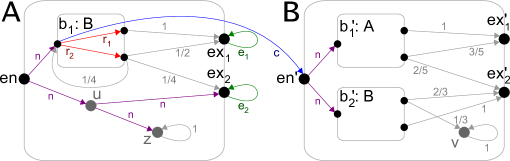
Figure 3: Example RMDP with Call, Return, and Exit edges added to $A$

Termination of $1$-RMDPs can be encoded as the following separable formula:

$$\psi_{1}=\mu X.\langle e_{1}\rangle\mathsf{tt}\lor\langle p\rangle X\lor\langle n\rangle X\lor(\langle c\rangle X\land\langle r_{1}\rangle X)$$ (16)

Termination of multi-exit RMDPs is undecidable, in general [13]. We can still encode it in XPL, but the resulting formula is not separable: the termination formula for a $2$-exit RMDP (17) is entangled on the $c$ action.

$$\psi_{2}^{1}=_{\mu}\langle e_{1}\rangle\mathsf{tt}\lor\langle p\rangle\psi_{2}^{1}\lor\langle n\rangle\psi_{2}^{1} \lor(\langle c\rangle\psi_{2}^{1}\land\langle r_{1}\rangle\psi_{2}^{1})$$ (17)

$$\lor(\langle c\rangle\psi_{2}^{2}\land\langle r_{2}\rangle\psi_{2}^{1})$$

$$\psi_{2}^{2}=_{\mu}\langle e_{2}\rangle\mathsf{tt}\lor\langle p\rangle\psi_{2}^{2}\lor\langle n\rangle\psi_{2}^{2} \lor(\langle c\rangle\psi_{2}^{1}\land\langle r_{1}\rangle\psi_{2}^{2})$$

$$\lor(\langle c\rangle\psi_{2}^{2}\land\langle r_{2}\rangle\psi_{2}^{2})$$

We note that the conjunction $\langle c\rangle X\land\langle r_{1}\rangle X$ in (16) is independent. Additionally, the disjunction between the two conjuncts in (17) is mutually exclusive, since $\langle c\rangle\psi_{1}^{2}$ and $\langle c\rangle\psi_{2}^{2}$ correspond to eventually reaching distinct exits; however, it is correct to sum them only for RMCs, as the nondeterministic choices in RMDPs preclude the simple summation of mutually exclusive outcomes.

5.3 PTTL and Branching Processes

PCTL* [2] may be considered a linear-time logic, in the sense that its fuzzy formulae are essentially full LTL. Similarly, PCTL [17] is not the only plausible extension of CTL: instead of replacing the $\mathsf{A}$ and $\mathsf{E}$ operators with the $\mathsf{Pr}$ operators, we could have full CTL as fuzzy formulae, as there is a natural interpretation of CTL over d-trees, and this logic, over RPLTS, would be subsumed by GPL.

A similar logic, Probabilistic Tree Temporal Logic (PTTL), has been independently introduced [4]. Branching Processes (BPs) are a branching-time extension of Markov chains, and PTTL is a logic over BPs. The problem of BP extinction corresponds to termination of $1$-exit RMCs [12]. BPs have also been extended with nondeterminism, yielding Branching MDPs (BMDPs), for which the extinction and reachability problems have been analyzed [11, 13].

We write the syntax of PTTL [4, Definition $18$], where $A\in Prop$, and we refer to $\phi$ and $\psi$ as state and fuzzy formulae, as for XPL:

$$\begin{array}[]{l}\phi::=A\mid\neg\phi\mid\phi\land\phi\mid\mathsf{Pr}_{>p}\psi\mid\mathsf{Pr}_{\geq p}\psi\\ \psi::=\mathsf{AX}\phi\mid\mathsf{EX}\phi\mid\mathsf{A}[\phi\mathsf{U}\phi]\mid\mathsf{E}[\phi\mathsf{U}\phi]\mid\mathsf{A}[\phi\mathsf{R}\phi]\mid\mathsf{E}[\phi\mathsf{R}\phi]\end{array}$$

In this section, we may view BPs as specialized RPLTSs, and RMDPs as specialized PLTSs. So, we give the semantics for PTTL over PLTSs (without terminal states), assuming maximizing schedulers, by encoding it in XPL, as $E_{PTTL}(\gamma)$, in Table 5.

Table 5: Encoding of PTTL over BMDPs

$$E_{PTTL}(\gamma)=\left\{\begin{array}[]{ll}\hline\cr\gamma,&\gamma\in Prop,\\ \mathsf{neg}(E_{PTTL}(\gamma^{\prime})),&\gamma=\neg\gamma^{\prime},\\ E_{PTTL}(\gamma_{1})\land E_{PTTL}(\gamma_{2}),&\gamma=\gamma_{1}\land\gamma_{2},\\ \mathsf{Pr}_{>p}E_{PTTL}(\psi),&\gamma=\mathsf{Pr}_{>p}\psi,\\ \mathsf{Pr}_{\geq p}E_{PTTL}(\psi),&\gamma=\mathsf{Pr}_{\geq p}\psi,\\ [-]E_{PTTL}(\phi),&\gamma=\mathsf{AX}\phi,\\ \langle-\rangle E_{PTTL}(\phi),&\gamma=\mathsf{EX}\phi,\\ \mu X.E_{PTTL}(\phi_{2})\lor(E_{PTTL}(\phi_{1})\land[-]X),&\gamma=\mathsf{A}[\phi_{1}\mathsf{U}\phi_{2}],\\ \mu X.E_{PTTL}(\phi_{2})\lor(E_{PTTL}(\phi_{1})\land\langle-\rangle X),&\gamma=\mathsf{E}[\phi_{1}\mathsf{U}\phi_{2}],\\ \nu X.E_{PTTL}(\phi_{2})\land(E_{PTTL}(\phi_{1})\lor[-]X),&\gamma=\mathsf{A}[\phi_{1}\mbox{\sf R}\phi_{2}].\\ \nu X.E_{PTTL}(\phi_{2})\land(E_{PTTL}(\phi_{1})\lor\langle-\rangle X),&\gamma=\mathsf{E}[\phi_{1}\mbox{\sf R}\phi_{2}].\\ \hline\cr\end{array}\right.$$

This translation also concretely demonstrates how the branching-time nature of GPL and XPL has not been recognized: either unnoticed (“the existing model-checking algorithms do not work for branching processes” [4]) or misunderstood (“it cannot express $\dots$ the CTL formula $\mathsf{EG}p$” [3] — but, through PTTL, it can).

6 Discussion and Future Work

Previous attempts to extend GPL included allowing systems with internal nondeterminism while still resolving the probabilistic choices first [5], and EGPL, which had similar syntax and semantics to XPL, but limited the model checking to non-recursive formulae [28].

Following GPL, XPL treats conjunction in a traditional manner, retaining the properties that $\psi\land\neg\psi=\mbox{\sf ff}$, and $\psi\land\psi=\psi$ for any formula $\psi$. However, the probability value of $\psi_{1}\land\psi_{2}$ cannot be computed based on the probability values of the conjuncts $\psi_{1}$ and $\psi_{2}$. This makes model checking in XPL more complex, but also contributes to its expressiveness.

Another probabilistic extension of $\mu$-calculus is pL$\mu$. In contrast to XPL, the most expressive version of pL$\mu$, denoted pL$\mu^{\odot}_{\oplus}$ [22, 23], defines three conjunction operators and their duals such that their probability values can be computed from the probabilities of the conjuncts. The logic pL$\mu^{\odot}$ is able to support branching time and an intuitive game semantics [22]. Along the same lines as our XPL encoding, we can encode termination of $1$-exit RMDPs as model checking in pL$\mu^{\odot}$, and RMC termination in pL$\mu^{\odot}_{\oplus}$. However, attempting to encode multi-exit RMDP termination in pL$\mu^{\odot}_{\oplus}$ similarly to multi-exit RMC termination would lead to an incorrect, rather than undecidable, encoding. Determining the relationship between XPL and pL$\mu^{\odot}$ in branching time is an important problem. Other recent probabilistic extensions of $\mu$-calculus include the Lukasiewicz $\mu$-calculus [24] and $\mu^{p}$-calculus [3], which can encode PCTL* over MDPs, and P$\mu$TL [19], but all these limit nondeterminism to the linear-time semantics. Quantitative $\mu$-calculi, such as qM$\mu$ [20] and Q$\mu$ [14], are more similar to pL$\mu$, so we do not offer an independent comparison to XPL.

Although closely related, algorithms to check properties of RMCs (and pPDSs [8]) were developed independently [12]. These were related to algorithms for computing properties of systems such as branching process (BP) extinction and the language probability of Stochastic Context Free Grammars. The relationship between GPL and these systems was mentioned briefly in [16], but has remained largely unexplored.

There has been significant interest in the study of expressive systems with nondeterministic choices, such as RMDPs and Branching MDP (BMDPs) [13]. At the same time, the understanding of the polynomial systems has expanded. In [9], the class of Probabilistic Polynomial Systems (PPS) is introduced, which characterizes when efficient solutions to polynomial equation systems are possible even in the worst case [10]. While [12] did not distinguish the systems arising from $1$-exit RMCs from those from multi-exit RMCs, the PPS class is limited to $1$-exit RMCs. It was also extended for RMDP termination and, later, BMDP reachability, both having polynomial-time complexity for min/maxPPSs [9, 11].

Systems producing equations in PPS form show an interesting characteristic: that the properties are expressible as purely conjunctive or purely disjunctive formulae. Recall that such formulae are trivially separable. Polynomial systems equivalent to those arising from separable GPL have recently been considered in a more general setting in the context of game automata [21], followed by an undecidability result for more general properties on the automata [25]. Characterizing equation systems that arise from separable formulae and investigating their efficient solution is an interesting open problem. Finally, this paper addressed the decidability of model checking; determining the complexity of model checking is a topic of future research.

References

- [1] Rajeev Alur, Swarat Chaudhuri, and P. Madhusudan. Software model checking using languages of nested trees. ACM Trans. Program. Lang. Syst., 33(5):15:1–15:45, November 2011.
- [2] Christel Baier. On algorithmic verification methods for probabilistic systems. Habilitation thesis, Fakultät für Mathematik & Informatik, Universität Mannheim, 1998.
- [3] Pablo Castro, Cecilia Kilmurray, and Nir Piterman. Tractable probabilistic mu-calculus that expresses probabilistic temporal logics. In STACS, volume 30 of LIPIcs, pages 211–223. Schloss Dagstuhl–Leibniz-Zentrum fuer Informatik, 2015.
- [4] Taolue Chen, Klaus Dräger, and Stefan Kiefer. Model checking stochastic branching processes. In MFCS, pages 271–282, Berlin, Heidelberg, 2012. Springer.
- [5] Rance Cleaveland and S Purushothaman Iyer. Branching time probabilistic model checking. In ICALP Workshops, volume 8, pages 487–500. Citeseer, 2000.
- [6] Rance Cleaveland, S. Purushothaman Iyer, and Murali Narasimha. Probabilistic temporal logics via the modal mu-calculus. Theoretical Computer Science, 342(2-3):316–350, 2005.
- [7] Josée Desharnais, Vineet Gupta, Radha Jagadeesan, and Prakash Panangaden. Weak bisimulation is sound and complete for PCTL*. In CONCUR, volume 2421 of LNCS, pages 355–370. Springer Berlin Heidelberg, 2002.
- [8] Javier Esparza, Antonín Kucera, and Richard Mayr. Model checking probabilistic pushdown automata. In LICS, pages 12–21, 2004.
- [9] Kousha Etessami, Alistair Stewart, and Mihalis Yannakakis. Polynomial time algorithms for branching Markov decision processes and probabilistic min(max) polynomial Bellman equations. In ICALP, Part I, pages 314–326, Berlin, Heidelberg, 2012. Springer.
- [10] Kousha Etessami, Alistair Stewart, and Mihalis Yannakakis. Polynomial time algorithms for multi-type branching processes and stochastic context-free grammars. In STOC, pages 579–588. ACM, 2012.
- [11] Kousha Etessami, Alistair Stewart, and Mihalis Yannakakis. Greatest fixed points of probabilistic min/max polynomial equations, and reachability for branching Markov decision processes. In ICALP, Part II, pages 184–196, Berlin, Heidelberg, 2015. Springer.
- [12] Kousha Etessami and Mihalis Yannakakis. Recursive Markov chains, stochastic grammars, and monotone systems of nonlinear equations. J. ACM, 56(1):1:1–1:66, February 2009.
- [13] Kousha Etessami and Mihalis Yannakakis. Recursive Markov decision processes and recursive stochastic games. J. ACM, 62(2):11:1–11:69, May 2015.
- [14] Diana Fischer, Erich Grädel, and Łukasz Kaiser. Model checking games for the quantitative -calculus. Theory of Computing Systems, 47(3):696–719, 2010.
- [15] Andrey Gorlin and C. R. Ramakrishnan. XPL: an extended probabilistic logic for probabilistic transition systems. CoRR, abs/1604.06118, 2016.
- [16] Andrey Gorlin, C. R. Ramakrishnan, and Scott A. Smolka. Model checking with probabilistic tabled logic programming. TPLP, 12(4-5):681–700, 2012.
- [17] Hans Hansson and Bengt Jonsson. A logic for reasoning about time and reliability. Formal Aspects of Computing, 6(5):512–535, 1994.
- [18] Stefan Kiefer, Michael Luttenberger, and Javier Esparza. On the convergence of Newton’s method for monotone systems of polynomial equations. In STOC, pages 217–226, 2007.
- [19] Wanwei Liu, Lei Song, Ji Wang, and Lijun Zhang. A simple probabilistic extension of modal mu-calculus. In IJCAI, 2015.
- [20] Annabelle McIver and Carroll Morgan. Results on the quantitative -calculus qM. ACM Trans. Comput. Logic, 8(1), January 2007.
- [21] Henryk Michalewski and Matteo Mio. On the problem of computing the probability of regular sets of trees. In FSTTCS, volume 45 of LIPIcs, pages 489–502. Schloss Dagstuhl - Leibniz-Zentrum fuer Informatik, 2015.
- [22] Matteo Mio. Probabilistic modal -calculus with independent product. In FOSSACS, volume 6604 of LNCS, pages 290–304. Springer, 2011. doi:10.1007/978-3-642-19805-2_20.
- [23] Matteo Mio. Game semantics for probabilistic modal mu-calculi. PhD thesis, The University of Edinburgh, 2012.
- [24] Matteo Mio and Alex Simpson. Łukasiewicz mu-calculus. In FICS, volume 126 of EPTCS, pages 87–104, 2013.
- [25] Marcin Przybylko and Michal Skrzypczak. On the complexity of branching games with regular conditions. In LIPIcs, volume 58. Schloss Dagstuhl-Leibniz-Zentrum fuer Informatik, 2016.
- [26] Roberto Segala. A compositional trace-based semantics for probabilistic automata. In CONCUR, volume 962 of LNCS, pages 234–248. Springer, 1995.
- [27] Roberto Segala and Andrea Turrini. Comparative analysis of bisimulation relations on alternating and non-alternating probabilistic models. In QEST, pages 44–53. IEEE Computer Society, 2005.
- [28] Arvind Soni. Probabilistic and nondeterministic systems. Masters thesis, North Carolina State University, 2004.
- [29] Alfred Tarski. A decision method for elementary algebra and geometry. Bulletin of the American Mathematical Society, 59, 1951.