Chandra and XMM-Newton X-Ray Observations of the Hyperactive T Tauri Star RY Tau

Abstract

We present results of pointed X-ray observations of the accreting jet-driving T Tauri star RY Tau using Chandra and XMM-Newton. We obtained high-resolution grating spectra and excellent-quality CCD spectra and light curves with the objective of identifying the physical mechanisms underlying RY Tau’s bright X-ray emission. Grating spectra reveal numerous emission lines spanning a broad range of temperature superimposed on a hot continuum. The X-ray emission measure distribution is dominated by very hot plasma at T_hot $\sim$ 50 MK but higher temperatures were present during flares. A weaker cool plasma component is also present as revealed by low-temperature lines such as O VIII. X-ray light curves show complex variability consisting of short-duration ($\sim$hours) superhot flares accompanied by fluorescent Fe emission at 6.4 keV superimposed on a slowly-varying ($\sim$one day) component that may be tied to stellar rotation. The hot flaring component is undoubtedly of magnetic (e.g. coronal) origin. Soft and hard-band light curves undergo similar slow variability implying that at least some of the cool plasma shares a common magnetic origin with the hot plasma. Any contribution to the X-ray emission from cool shocked plasma is small compared to the dominant hot component but production of individual low-temperature lines such as O VIII in an accretion shock is not ruled out.

1 Introduction

Classical T Tauri stars (cTTS) are low-mass pre-main sequence stars that are accreting from disks and continue to be high-interest objects for their remarkable range of activity (Bertout 1989) and as potential host stars for nascent protoplanetary systems. They are intense X-ray emitters whose X-ray luminosities typically exceed that of the contemporary Sun by $\sim$2-3 orders of magnitude (Feigelson & Montmerle 1999). The intense X-ray emission heats and ionizes the inner disk, altering disk chemistry and influencing the physical environment in which planet formation occurs (Glassgold et al. 1997; Shang et al. 2002).

Early studies of cTTS suggested that their X-ray emission is dominated by magnetic (e.g. coronal) processes analogous to scaled-up solar activity (Feigelson & Montmerle 1999). This emission is often variable and can display huge magnetic reconnection flares characterized by rapid changes ($\sim$hours to days) in the observed X-ray flux and elevated plasma temperatures reaching extreme values T $\,\stackrel{{\scriptstyle\raisebox{-0.60275pt}{$\textstyle>$}}}{{\sim}}\,$ 100 MK.

However, more recent observational work has shown that other physical processes also contribute to the X-ray emission of cTTS. Cool plasma (T $<$ 3 MK) that is thought to arise in the post-shock zone of an accretion shock at or near the stellar surface has been detected in a few cTTS, most notably TW Hya (Kastner et al. 2002; Stelzer & Schmitt 2004; Brickhouse et al. 2010). There is also accumulating evidence that faint soft X-rays are produced in collimated high-speed jets within a few arcseconds of the central star. Such cTTS X-ray jet sources include the well-studied object DG Tau (Güdel et al. 2005; 2008) and possible X-ray jet detections in RY Tau (Skinner, Audard, & Güdel 2011; hereafter SAG11) and RW Aur (Skinner & Güdel 2014). X-ray jet emission was also observed following an optical outburst in the unusual pre-main sequence binary Z CMa (Stelzer et al. 2009). Soft X-ray emission that likely originates in shock-heated material has been reported in some Herbig-Haro objects of which a few examples are HH 2 (Pravdo et al. 2001), HH 80/81 (Pravdo et al. 2004), HH 154 (Favata et al. 2002, 2006; Bally et al. 2003), and HH 210 (Grosso et al. 2006).

X-ray jet emission is usually recognized in high-resolution images as $\sim$arcsecond-scale structure extending outward from the unresolved central star along one or (rarely) both of the optical jet axes. Chandra’s excellent spatial resolution has proven to be especially useful in identifying such faint extended jet structure. On the other hand, coronal and accretion shock X-ray emission originate near the stellar surface and cannot be spatially resolved with existing X-ray telescopes. But analysis of individual emission lines in high-resolution X-ray grating spectra can potentially distinguish between cool dense plasma in accretion shocks (T $\sim$ few MK; n_e $\,\stackrel{{\scriptstyle\raisebox{-0.60275pt}{$\textstyle>$}}}{{\sim}}\,$ 10¹² cm^-3) and hotter lower density coronal plasma (typically n_e $\,\stackrel{{\scriptstyle\raisebox{-0.60275pt}{$\textstyle<$}}}{{\sim}}\,$ 10¹² cm^-3), as clearly demonstrated in the case of TW Hya.

Relatively few cTTS are bright enough in X-rays to permit good-quality grating spectra to be acquired in reasonable exposure times. We identified the accreting jet-driving cTTS RY Tau as a promising candidate for grating spectroscopy on the basis of bright X-ray emission detected in a 2009 Chandra ACIS-S observation (SAG11). Moderate resolution CCD spectra revealed multi-temperature plasma consisting of a superhot flaring component (typical of coronal emission) and cooler plasma of uncertain origin. Deconvolved soft-band images showed some evidence of extension outward along the blueshifted optical jet.

We present here new X-ray observations of the cTTS RY Tau obtained with Chandra and XMM-Newton. These observations include the first high-resolution grating spectra of RY Tau as well as high-quality undispersed CCD spectra and X-ray light curves. Our main objective is to obtain a more complete picture of the properties of the X-ray emitting plasma (i.e. temperature, electron density, emission measure distribution) in order to differentiate between hot magnetically-confined plasma (e.g. coronal emission) and cooler plasma that may originate in shocks.

Table 1: Properties of RY Tau

Sp. Type	M∗	V	AV	L∗	Lbol	log Lx	log $\dot{M}_{acc}$	d
	(M⊙)	(mag)	(mag)	(L⊙)	(L⊙)	(ergs s-1)	(M⊙ yr-1)	(pc)
F8 III - G3 IV	1.7 - 2.0	9.3 - 11 (v)	2.2$\pm$0.2	7.0 - 8.8	15.3	30.5 - 31.2(v)	$-$7.3$\pm$0.3	134

Note. — Data are from Agra-Amboage et al. (2009), Calvet et al. (2004), Holtzman et al. (1986), Kenyon & Hartmann (1995), and Schegerer et al. (2008). The stellar luminosity L_∗ and bolometric luminosity L_bol are based on the values L_∗ = 7.6 - 9.6 L_⊙ and L_bol = 16.7 L_⊙ at d = 140 pc (Calvet et al. 2004, Kenyon & Hartmann 1995) and have been normalized to d = 134 pc. L_x range is based on this work. Distance is from Bertout et al. (1999). Variable parameters are denoted by (v). Spectral type is uncertain (Holtzman, Herbst, & Booth 1986).

2 RY Tau

RY Tau is an optically variable cTTS lying in the Taurus dark cloud (Bertout, Robichon, & Arenou 1999). Its properties are summarized in Table 1. Its mass M_∗ $\approx$ 2 M_⊙ is relatively high for a TTS and it rotates rapidly at $v$sin$i$ = 52 $\pm$ 2 km s^-1 (Petrov et al. 1999). It is accreting from a disk (Schegerer et al. 2008; Angra-Amboage et al. 2009) and mass-loss is clearly evident in the form of a bipolar jet known as HH 938 (St.-Onge & Bastien 2008) and a wind (Gómez de Castro & Verdugo 2007). Optical images have traced the jet and associated H$\alpha$ knots outward to a separation of 31^′′ from the star along P.A. $\approx$ 295^∘ (measured east from north), and the fainter counterjet is visible out to 3.^′5 from the star. Binarity is suspected based on Hipparcos photocenter motions (Bertout et al. 1999) but no companion has yet been found (Leinert et al. 1993; Schegerer et al. 2008; Pott et al. 2010). Searches for periodic optical variability have reported periods of $\sim$years but no stable short period of $\sim$days that might be associated with stellar rotation has yet been confirmed (Bouvier et al. 1993; Ismailov & Adygezalzade 2012 and references therein; Zajtseva 2010).

3 Summary of Previous XMM-Newton and Chandra Observations

2000: RY Tau was captured 8.5^′ off-axis in a September 2000 XMM-Newton observation targeted on HDE 283572 (51 ks; ObsId 0101440701). This archived observation was included in the XMM-Newton Extended Survey of the Taurus Molecular Cloud (XEST) as reported by Güdel et al. (2007a). RY Tau was cataloged as XEST source 21-038. Fits of its CCD spectra with an absorbed 2T thermal plasma model gave N_H = 7.6 ($+$0.9,$-$1.0) $\times$ 10²¹ cm^-2, kT_cool = 0.5 keV, kT_hot = 3.2 keV, and log L_x(0.3 - 10 keV) = 30.72 ergs s^-1 (d = 140 pc). No large-amplitude variability was reported.

2003: RY Tau was captured off-axis in a October 2003 Chandra ACIS-S/HETG grating observation targeted on HDE 283572 (ObsId 3756). The zero-order ACIS-S spectrum and light curve of RY Tau were analyzed by Audard et al. (2005) but the grating spectrum was not analyzed due to lack of reliable calibration for far off-axis sources. The $\approx$100 ks X-ray light curve showed a slow decline punctuated by a short-duration low-amplitude flare. The ACIS-S spectrum was fitted with an absorbed two-temperature (2T) thermal plasma model with temperatures kT_cool = 1.0 keV, kT_hot = 3.9 keV, absorption N_H = 5 ($\pm$1) $\times$ 10²¹ cm^-2, subsolar metallicity $Z$ = 0.3 Z_⊙, and X-ray luminosity log L_x (0.1 - 10 keV) = 30.88 ergs s^-1 at d = 140 pc. Fluorescent Fe emission was detected at $\approx$6.4 keV.

2009: We obtained a 56 ks observation with RY Tau on-axis using Chandra ACIS-S without gratings in December 2009 (ObsId 10991). The star was detected as a bright variable X-ray source (SAG11). An absorbed 2T thermal plasma model gave N_H = 5.5 ($+$1.3,$-$0.8) $\times$ 10²¹ cm^-2, kT_cool = 0.6 keV, kT_hot = 4.8 keV, $Z$ = 0.25 Z_⊙, and log L_x(0.2 - 10 keV) = 30.67 ergs s^-1 (d = 134 pc). For comparison with the above studies, the latter value equates to log L_x = 30.71 ergs s^-1 at d = 140 pc. Deconvolved soft-band (0.2 - 2 keV) ACIS-S images revealed faint extended structure overlapping the inner blushifted optical jet and traced out to a separation of $\approx$1.^′′7 from the star. A known asymmetry in the Chandra point-spread function may contribute to some of the structure inside one arcsecond. Five other X-ray sources were detected within one arcminute of RY Tau but all were quite faint.

Table 2: RY Tau X-ray Observations

Telescope	XMM-Newton	Chandra	Chandra
Date	2013 Aug. 21-22	2014 Oct. 22-23	2014 Oct. 23-24
ObsId	0722320101	15722	17539
Start Time (UTC)	04:34	02:06	21:37
Stop Time (UTC)	11:13	03:06	04:49
Duration (ks)	92.25	85.5	23.9
Prime Instrument	RGS	ACIS-S/HETG	ACIS-S/HETG

4 Observations and Data Reduction

The X-ray observations are summarized in Table 2.

4.1 XMM-Newton

The XMM-Newton data were obtained in a single observation spanning $\approx$31 hours in August 2013. The primary instrument was the Reflection Grating Spectrometer (RGS) which consists of two spectrometers (RGS1 and RGS2) with similar spectral coverage over the $\approx$0.35 - 2.5 keV energy range but with some gaps. The RGS effective area in first order reaches a maximum of $\approx$50 - 60 cm² per RGS at $\approx$15 Å ($\approx$0.8 keV), thus providing better sensitivity at lower energies $\,\stackrel{{\scriptstyle\raisebox{-0.60275pt}{$\textstyle<$}}}{{\sim}}\,$1 keV than the Chandra High Energy Transmission Grating (HETG). RGS first order spectral resolution at 12 Å ($\approx$1 keV) is $\Delta\lambda$ $\approx$ 0.055 - 0.07 Å (FWHM). In addition, XMM-Newton provided CCD imaging spectroscopy from the European Photon Imaging Camera (EPIC) which was used with the Medium optical filter. The EPIC consists of the pn camera and two nearly-identical MOS cameras (MOS1 and MOS2; Turner et al. 2001). The EPIC cameras provide energy coverage in the range E $\approx$ 0.2 - 15 keV with energy resolution (FWHM) at 1 keV of $\Delta E$ $\approx$ 70 eV (MOS) and $\Delta E$ $\approx$ 100 eV (pn).

Data were reduced using the XMM-Newton Science Analysis System (SAS vers. 13.5.0). Event files were time-filtered to remove data acquired during a background flare at the end of the observation, resulting in $\approx$90 - 100 ks of usable exposure per instrument (Table 2). EPIC spectra and energy-filtered light curves were extracted from a circular region of radius 20^′′ centered on the source and background was extracted from source-free regions near RY Tau. The SAS task $rgsproc$ produced edited RGS event files that excluded the high-background time interval. RGS response matrix files (RMFs) were generated using the SAS task $rgsrmfgen$. Spectra were analyzed with Sherpa in CIAO version 4.6 and with XSPEC version 12.8.2. Timing analysis was performed with XRONOS v. 5.22. XSPEC and XRONOS are included in the HEASOFT XANADU software package.

4.2 Chandra

The Chandra data were acquired with the HETG and ACIS-S detector array in October 2014 in two observations spanning $\approx$24 hours and $\approx$7 hours with an intervening gap of $\approx$18.5 hours (Table 2). The combined livetime of the two observations was 109.4 ks, of which 85.5 ks was obtained in the first observation. The nominal pointing direction and roll angle were nearly identical for the two observations. Five of the six CCDs in the ACIS-S array were enabled (chip S0 was turned off).

We analyzed dispersed first-order HETG spectra from the Medium Energy Grating (MEG) and High Energy Grating (HEG) as well as undispersed (zero-order) ACIS-S spectra and X-ray light curves. The data were processed using standard science threads in CIAO version 4.6 and associated calibration data from CALDB version 4.6.1.1. Our analysis is based on Level 2 event files provided by Chandra X-ray Center (CXC) standard processing.

The HETG provides spectral coverage over the $\approx$0.4 - 10 keV ($\approx$1.3 - 30 Å ) range. Background rejection is high in HETG because of event order discrimination by ACIS-S, in sharp contrast to the much higher background in XMM-Newton RGS spectra. In addition, HETG provides spectral coverage above 2.5 keV where RGS coverage is lacking and is thus crucial for diagnosing hot plasma. Spectral resolution in first order is $\Delta\lambda$ $\approx$ 0.023 Å  for MEG and $\Delta\lambda$ $\approx$ 0.012 Å  for HEG. The separate $+$1 and $-1$ order MEG spectra were co-added for analysis, and similarly for HEG. The effective area of MEG is maximum between 1 - 2 keV and HEG is maximum between 2 - 3 keV. The effective area of both gratings is lower than RGS at energies $<$1 keV. The HEG has superior spectral resolution but the MEG provides more total counts and higher signal-to-noise ratio in first-order spectra for this observation. Our Chandra grating analysis thus emphasizes the MEG spectrum for the longer first exposure (ObsId 15722) when most of the source counts were accumulated.

The zero-order ACIS-S CCD spectra and X-ray light curves were extracted from a circular region of radius 2^′′ centered on the RY Tau source peak. Background is negligible. ACIS-S provides energy coverage from $\approx$0.4 - 10 keV and its intrinsic energy resolution is $\Delta E$ $\approx$ 120 eV (FWHM) at E = 1 keV. Unlike our previous 2009 Chandra ACIS-S observation (without gratings), no 0-order image deconvolution was performed for the new ACIS-S/HETG observation discussed here. The point-spread-function (PSF) needed to produce the deconvolved image is spectral-dependent and the spectrum varied considerably throughout the observation (Sec. 5.2). In addition, the gratings disperse a significant fraction of the incoming photons, especially at energies below 2 keV, thereby reducing the sensitivity in 0-order to any faint soft ($<$2 keV) extended X-ray jet emission at small offsets from the star.

5 Results

5.1 X-ray Light Curves and Variability

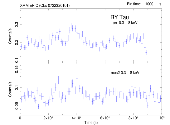
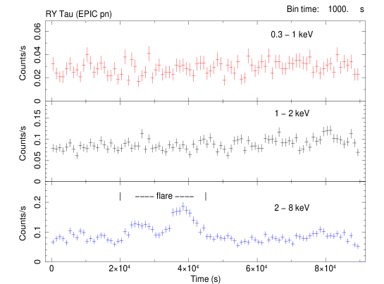
Figure 1: Background-subtracted XMM-Newton EPIC light curves of RY Tau (1000 s time bins). Times are relative to the start of the observation.  Top: EPIC pn and MOS2 broad-band light curves (0.3 - 8 keV).  Bottom: EPIC pn light curves in three different energy bands. No significant variability is present in the very soft energy band (0.3 - 1 keV) but the medium (1 - 2 keV) and hard (2 - 8 keV) band light curves are variable with high probability P_var $>$ 0.99. A separate spectrum was extracted for the interval marked ‘flare’ in the hard-band light curve.

The XMM-Newton EPIC broad-band light curves (Fig. 1-top) are clearly variable during the first half of the observation. Two flare-like outbursts occurred within the time interval $\sim$20 - 45 ks after the start of the observation. EPIC spectra extracted during these flare intervals (Sec. 5.2) give substantially higher mean plasma temperatures than obtained from spectra extracted after removing the flares. Energy-filtered pn light curves (Fig. 1-bottom) show no significant variability in the very soft band (0.3 - 1 keV) but have a high probability of variability P_var $>$ 0.99 in the medium (1 - 2 keV) and hard (2 - 8 keV) bands. The medium-band light curve reveals a slow increase in count rate during the observation with an average rate of 82$\pm$2 c ks^-1 in the first half and 92$\pm$2 c ks^-1 in the second half. Flare-like variability is most obvious in the hard band.

The Chandra ACIS-S 0-order light curves are also variable. As shown in Fig. 2-top left, a slow decrease in count rate occurred during the first 40 ks of the first observation (ObsId 15722), followed by a moderate slow increase. The slow decay and subsequent rise are clearly detected in the very soft, medium, and hard energy bands (Fig. 2-bottom left). An exponential fit of the decay portion of the broad-band (0.3 - 8 keV) ACIS-S light curve gives an e-folding time of 27.5 ks. The plasma temperature and X-ray flux decreased during the decay phase and then began to increase again after the light curve minimum, as discussed further in Sec. 6.

The average count rate and plasma temperature were lower in the second Chandra observation (ObsId 17539). A slow decrease in the broad-band (0.3 - 8 keV) and hard-band (2 - 8 keV) count rates is clearly visible (Fig. 2-right). There are insufficient counts to construct a separate very-soft band (0.3 - 1 keV) light curve so a 0.3 - 2 keV band light curve was generated to search for low-energy variability. This light curve is nearly constant during the first half of the observation but declines during the second half (Fig. 2-bottom right). The respective count rates in the first and second halves were 9.42 $\pm$ 0.89 c ks^-1 and 8.08 $\pm$ 1.86 c ks^-1 (1$\sigma$ uncertainties). A $\chi^{2}$ test applied to the second half of the observation gives a variability probability P_var = 0.60 which is suggestive of variability but not conclusive.

5.2 Undispersed CCD X-ray Spectra

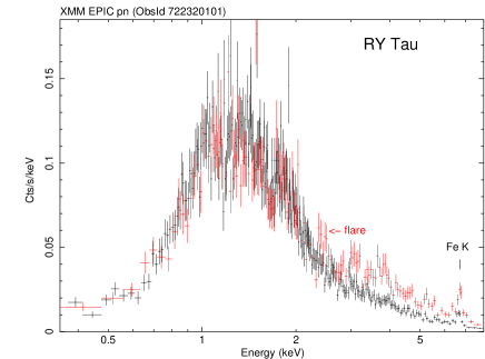
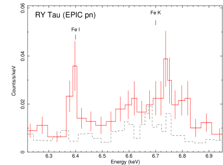
Figure 3: Top: XMM EPIC pn spectra of RY Tau binned to a minimum of 40 counts per bin. The flare spectrum (red) includes only events recorded in the 25 ks flare segment (see Fig. 1). The quiescent spectrum is based on 65 ks of exposure that excludes the flare. Both spectra exclude high background data at the end of the observation.  Bottom: XMM EPIC pn flare (solid) and flare-excluded (dashed) spectra of RY Tau binned to a minimum of 10 counts per bin. The flare spectrum shows emission from the Fe K line complex which includes multiple Fe XXV transitions near 6.7 keV arising in very hot plasma and fluorescent Fe emission near 6.4 keV originating in cold irradiated material. The EPIC pn energy resolution at 6.7 keV is FWHM $\approx$ 0.15 keV.

Figure 3 shows the XMM-Newton EPIC pn spectra, which provide higher count rates and better sensitivity at low energies than MOS spectra. Spectra for the flare and non-flare time intervals are overlaid. The flare spectrum extracted during the 25 ks flare interval (as marked in the bottom panel of Fig. 1) is clearly harder as evidenced by elevated continuum emission above $\sim$2 keV. The ratio H/S of hard-band (2 - 8 keV) to soft-band (0.3 - 2 keV) EPIC pn counts during the flare segment was H/S = 1.10 as compared to H/S = 0.67 during the non-flare time interval. The Fe K line complex near 6.7 keV (Fe XXV) which originates in very hot plasma (maximum emissivity temperature T_e,max $\approx$ 63 MK) is present in both the flare and flare-excluded segments. Interestingly, an emission feature at $\approx$6.4 keV is present in the flare spectrum (Fig. 3-bottom). A Gaussian fit of this feature gives a centroid energy E = 6.395 $\pm$ 0.005 (1$\sigma$) keV. This line is fluorescent emission from neutral or near-neutral Fe irradiated by the hard flaring X-ray source.

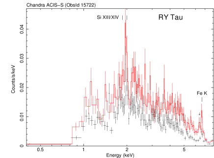
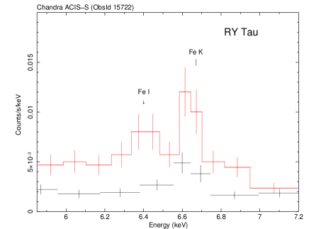
Figure 4: Top: Chandra ACIS-S 0-order spectra of RY Tau for ObsId 15722 binned to a minimum of 20 counts per bin. The spectrum connected by the solid histogram (red) consists of 2763 counts recorded in the first 35 ks of the observation (high-state) when the count rate was high and slowly decaying. The spectrum without the histogram line (black) consists of 2338 counts recorded during the low-state from t = 35 ks to the end of the observation (duration 52.586 ks). Arrow marks probable fluorescent Fe emission at 6.4 keV. Bottom: Same as top showing a more detailed view of the Fe lines between 6.4 - 6.7 keV. The ACIS chip S3 energy resolution from pre-launch measurements is FWHM $\approx$ 0.2 keV at 6.7 keV.

Figure 4 shows the undispersed ACIS-S spectra extracted during the first Chandra observation (ObsId 15722). The spectrum corresponding to the first 35 ks of the observation when the count rate was higher (“high state”) is overlaid on that of the remaining $\sim$50 ks segment (“low state”). The spectrum is slightly harder during the high state with a hardness ratio H/S = 3.17 as compared to H/S = 2.84 in the low-state. The Fe K emission line complex is detected in both the high state and low state time segments. Similar to the EPIC pn spectrum, the ACIS-S spectrum extracted during the first 35 ks high-state segment reveals a weak emission feature near 6.4 keV that is undoubtedly fluorescent Fe emission (Fig. 4-bottom). A similar feature was present in the off-axis zero-order ACIS-S spectrum of RY Tau in 2003 (Audard et al. 2005).

5.2.1 Discrete Temperature Models

We fitted the undispersed spectra with absorbed $apec$ optically thin plasma models to obtain estimates of the absorption column density (N_H), mean plasma temperature (kT), metallicity ($Z$), X-ray flux (F_x), and unabsorbed X-ray luminosity (L_x). Separate fits were obtained for spectra extracted during flare intervals and intervals which excluded obvious flares, as summarized in Table 3. The 1T $apec$ models are overly simplistic in the sense that they only provide a mean temperature and don’t give information on how the plasma is distributed versus temperature. The distribution of plasma versus temperature is better assessed with differential emission measure models (Sec. 5.2.2).

Several conclusions can be reached by examining the fit results in Table 3. Despite the simplicity of the 1T $apec$ model, it gives a surprisingly good fit of the EPIC pn “quiescent” spectrum, with a mean temperature of kT = 4.35 keV and reduced chi-squared value $\chi^{2}_{\nu}$ = 1.02. A fit of the same spectrum with a two-temperature (2T) $apec$ model yields very little further improvement as gauged by the fit statistic (Table 3 Notes). This is a clear indication that the X-ray emission measure is dominated by hot plasma.

Mean temperatures were higher during flare segments. Very high temperatures occurred during the 25 ks flare segment in the XMM-Newton observation. Fitting the pn spectrum using combined data from both flare peaks gives kT_flare = 14.6 [11.3 - 17.9] keV. If spectra extracted for each flare peak are fitted separately, the second peak during which the hard band count rate reached a maximum yields a slightly higher temperature, but flare temperature uncertainties are large.

The X-ray luminosity is clearly variable. As Table 3 shows, the broad-band luminosity was highest during the high-state in the first $\sim$35 ks of the first Chandra observation (log L_x = 31.16 ergs s^-1). The luminosity during the second Chandra exposure (ObsId 17539) and the XMM-Newton observation were lower and comparable to the value log L_x = 30.67 ergs s^-1 obtained in 2009 December by Chandra (SAG11). Based on existing observations, the typical luminosity of RY Tau excluding flares is log L_x = 30.65 ($\pm$0.10) ergs s^-1. This is at the high end of the range observed for cTTS in Taurus (Fig. 1 of Telleschi et al. 2007a), as discussed further in Sec. 6.1.

All 1T $apec$ fits converge to subsolar metallicity with values in the range $Z$ $\approx$ 0.2 $Z_{\odot}$ (EPIC pn) to $Z$ $\approx$ 0.4 $Z_{\odot}$ (ACIS-S). Fits in which the abundances of individual elements were allowed to vary show that the low $Z$ values are driven by a low Fe abundance. A low Fe abundance is also obtained using differential emission measure models (Sec. 5.2.2).

X-ray absorption is best-determined from the EPIC pn spectra which provide better sensitivity at low energies $\,\stackrel{{\scriptstyle\raisebox{-0.60275pt}{$\textstyle<$}}}{{\sim}}\,$1 keV where absorption becomes important. The 1T $apec$ EPIC pn fit of the spectrum with the flare interval excluded (Table 3) gives a best-fit absorption N_H = 4.3 [4.1 - 4.4; 90% conf.] $\times$ 10²¹ cm^-2. A fit of the pn spectrum during the flare interval gives a nearly identical N_H value (Table 3). This above N_H is in good agreement with estimates based on optically-determined A_V = 2.2 $\pm$ 0.2 mag (Calvet et al. 2004) using the conversion N_H = 2.2$\times$ 10²¹A_V cm^-2 (Gorenstein 1975), which gives N_H = 4.8$\pm$0.4 $\times$ 10²¹cm^-2. By comparison, the conversion N_H = 1.6 $\times$ 10²¹A_V cm^-2 of Vuong et al. (2003), gives N_H = 3.5$\pm$0.3 $\times$ 10²¹cm^-2, slightly less than inferred from the EPIC pn fits. However, the value inferred for N_H is somewhat sensitive to the spectral model used and more sophisticated differential emission measure (DEM) models that allow for a range of plasma temperatures give somewhat larger N_H values, as discussed below.

Table 3: RY Tau Discrete Temperature Model Spectral Fits (0-order)

Parameter	Value
Telescope	CXO	CXO	CXO	XMM (pn)	XMM (pn)
ObsId	15722	15722	17539	722320101	722320101
Obs start date	22 Oct. 2014	22 Oct. 2014	23 Oct. 2014	21 Aug. 2013	21 Aug. 2013
Time interval (ks)	0.0 - 35.0	35.0 - 85.5	0.0 - 23.9	20.0 - 45.0	0.0 - 20.0, 45.0 - 90.0
Duration (ks)	35.0	50.5	23.9	25.0	65.0
State	high-decay	low-rise	low-decay	flares	non-flare
Model	1T $apec$	1T $apec$	1T $apec$	1T $apec$	1T $apec$
NH (1021 cm-2)	5.1 [4.7 - 6.0]	6.2 [5.3 - 7.5]	4.6 [3.0 - 6.8]	4.0 [3.7 - 4.3]	4.3 [4.1 - 4.4]
kT1 (keV)	7.66 [6.56 - 9.70]	4.56 [3.92 - 5.27]	2.88 [2.37 - 3.55]	14.6 [11.3 - 17.9]	4.35 [4.18 - 4.59]
norm1 (10-3 cm-5)	3.69 [3.45 - 3.92]	2.50 [2.26 - 2.80]	1.57 [1.29 - 1.95]	1.10 [1.07 - 1.13]	1.04 [1.00 - 1.07]
Abundances ($Z/Z_{\odot}$)	{0.4}	0.4 [0.26 - 0.52]	{0.4}	{0.2}	0.2 [0.16 - 0.27]
$\chi^{2}$/dof	138.5/116	132.1/98	28.9/24	389.6/262	487.6/479
$\chi^{2}_{\nu}$	1.19	1.35	1.20	1.49	1.02
Net counts (cts)	2755	2326	578	6132	13118
FX (10-12 ergs cm-2 s-1)	4.89 (6.70)	2.54 (3.94)	1.27 (2.10)	1.60 (2.07)	1.03 (1.59)
log LX (ergs s-1)	31.16	30.93	30.65	30.65	30.53

Note. — Based on XSPEC (vers. 12.8.2) fits of the background-subtracted ACIS-S and EPIC pn spectra binned to a minimum of 20 counts per bin. The tabulated spectral parameters are absorption column density (N_H), plasma energy (kT), and XSPEC component normalization (norm). Abundances are referenced to Anders & Grevesse (1989). Square brackets enclose 90% confidence intervals. Quantities enclosed in curly braces were held fixed during fitting. The total X-ray flux (F_X) is the absorbed value in the 0.2 - 10 keV range, followed in parentheses by unabsorbed value. The total X-ray luminosity L_X is the unabsorbed value in the 0.2 - 10 keV range and assumes a distance of 134 pc.

5.2.2 Differential Emission Measure Models

The 1T $apec$ models converge to high plasma temperatures T $\sim$ 50 MK (kT $\sim$ 4 - 5 keV) so the X-ray emission is undoubtedly dominated by very hot plasma. However, the presence of low-temperature emission lines in the grating spectra (Sec. 5.3) indicate that some cool plasma (T $\,\stackrel{{\scriptstyle\raisebox{-0.60275pt}{$\textstyle<$}}}{{\sim}}\,$ 10 MK) is also present. Differential emission measure (DEM) models allow for plasma distributed over a range of temperatures and thus provide a more realistic picture of the emission measure distribution than discrete-temperature models.

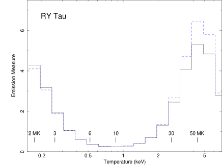
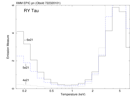
Figure 5: Top: Emission measure distribution of RY Tau obtained by fitting XMM-Newton spectra excluding the flare intervals. The fits were obtained with the XSPEC variable abundance model $c6pvmekl$ model (Table 4). The solid histogram is based on a fit of the EPIC pn spectrum and dashed histogram is based on a simultaneous fit of EPIC pn $+$ RGS1&2 spectra. The best-fit absorption is N_H = 6.0 $\times$ 10²¹ cm^-2. Bottom: A comparison of the emission measure distributions obtained by fitting the EPIC pn spectrum with the $c6pvmekl$ model using three different fixed values of N_H. Flare intervals were excluded. All three fits are acceptable with respective $\chi^{2}_{\nu}$ values 0.98 (N_H = 6e21 cm^-2), 0.99 (N_H = 5e21 cm^-2), and 1.02 (N_H = 4e21 cm^-2).

We have reconstructed the DEM using the variable abundance XSPEC model $c6pvmkl$ which is based on Chebyshev polynomials . We fitted the EPIC pn spectrum with this model, as well as a simultaneous fit of the EPIC pn spectrum plus the RGS1 and RGS2 spectra. Flare intervals were excluded in the interest of obtaining a picture of how the plasma is distributed during non-flaring (“quiescent”) conditions. Abundances of key elements with detected emission lines in the grating spectra were allowed to vary. Fit results are given in Table 4 and the derived DEM distribution from the best-fit model is shown in Figure 5-top. There are only minor differences between the DEM fit results obtained fitting the EPIC pn spectrum alone and by fitting the pn and RGS spectra simultaneously. This is a result of the much higher signal-to-noise ratio in the pn spectrum, which dominates the fit.

The DEM is dominated by a prominent peak at kT $\approx$ 4 - 5 keV as expected from the 1T $apec$ models. The high-temperature component is well-constrained by the continuum and several highly-ionized Fe lines. The DEM drops to a broad minimum near 1 keV (T $\sim$ 10 MK) and then rises slowly toward lower energies. The shape of the DEM below 1 keV is not tightly constrained because it is quite sensitive to absorption (N_H) which becomes important at low energies and suppresses low-energy emission. Figure 5-bottom illustrates how relatively small changes in absorption affect the derived shape of the cool plasma emission measure distribution. For the best-fit absorption determined by the $c6pvmkl$ model (N_H = 6 $\times$ 10²¹ cm^-2), the cool component rises steeply below 0.5 keV toward lower energies. But as N_H is decreased the cool component contributes less and becomes negligible if N_H = 4 $\times$ 10²¹ cm^-2. In addition to the sensitivity of the derived DEM to N_H, it is worth keeping in mind that the inverse modeling which underlies DEM reconstruction methods suffers from non-uniqueness issues, as has been discussed in previous studies (e.g. Judge & McIntosh 1999). Thus, the DEM reconstruction shown in Figure 5 should not be construed as unique.

The absorption determined from the variable-abundance DEM fit of the pn$+$RGS “quiescent” spectra is N_H = 6.0 [5.2 - 7.1; 90% conf.] $\times$ 10²¹ cm^-2, nearly identical to that obtained from 1T $apec$ fits of the ACIS-S low-state spectrum for ObsId 15722 (Table 3). It is also consistent with the value N_H = 5.5 [4.7 - 6.8] $\times$ 10²¹ cm^-2 obtained by Chandra ACIS-S in 2009 (SAG11) and in the 2003 Chandra off-axis exposure (Audard et al. 2005). The above absorption determinations are consistent with the value expected based on A_V = 2.2 $\pm$ 0.2 mag using the Gorenstein (1975) conversion which, as noted in Sec. 5.2.1, gives N_H = 4.8$\pm$0.4 $\times$ 10²¹cm^-2. But they are somewhat higher than the value N_H = 3.5$\pm$0.3 $\times$ 10²¹cm^-2 obtained using the Vuong et al. (2003) conversion. Thus, some excess X-ray absorption above that expected from A_V may be present.

The DEM model fit converges to a subsolar Fe abundance Fe = 0.31 [0.23 - 0.38; 90% confidence interval] $\times$ solar. The other elemental abundances are not as tightly constrained but O is also subsolar and the abundance ratio Ne/Fe $\approx$ 2.5 - 2.9 is similar to values reported for other TTS in Taurus including the prototype T Tau (Güdel et al. 2007b; Telleschi et al. 2007b). The above abundances are relative to the solar reference values of Anders & Grevesse (1989).

Table 4: RY Tau XMM-Newton DEM Model Spectral Fits

Parameter	Value
Spectra	pn	pn $+$ RGS1&2
ObsId	722320101	722320101
Time interval	quiescent	quiescent
Model	$c6pvmkl$	$c6pvmkl$
NH (1021 cm-2)	6.0 [5.0 - 6.8]	6.0 [5.2 - 7.1]
norm1 (10-4 cm-5)	0.46 [0.22 - 0.87]	0.40 [0.20 - 0.84]
Abundances	varied	varied
$\chi^{2}$/dof	453.6/469	551.2/541
$\chi^{2}_{\nu}$	0.97	1.02
FX (10-12 ergs cm-2 s-1)	1.04 (2.73)	1.04 (2.60)
log LX (ergs s-1)	30.77	30.75

Note. — Based on XSPEC (vers. 12.8.2) fits of the background-subtracted EPIC pn and RGS1&2 spectra using a variable-abundance $c6pvmkl$ model. Abundances are referenced to Anders & Grevesse (1989). Square brackets enclose 90% confidence intervals. The total X-ray flux (F_X) is the absorbed value in the 0.2 - 10 keV range, followed in parentheses by unabsorbed value. The total X-ray luminosity L_X is the unabsorbed value in the 0.2 - 10 keV range and assumes a distance of 134 pc.

5.3 X-ray Grating Spectra

5.3.1 XMM-Newton RGS

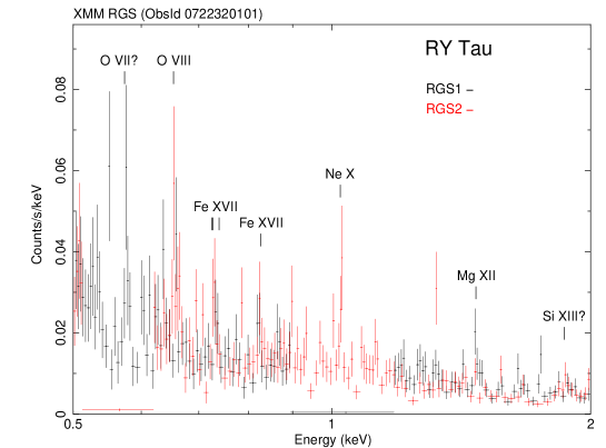
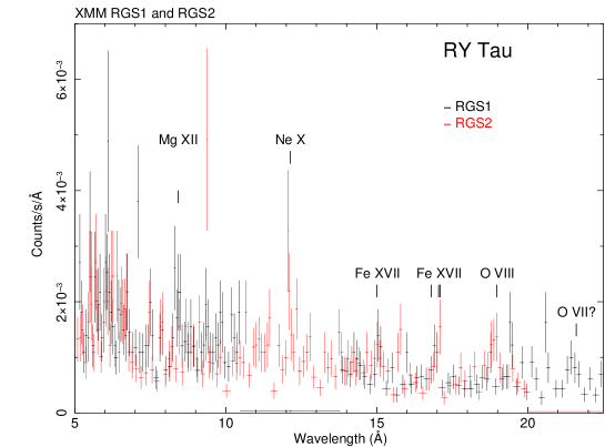
Figure 6:  Top: Binned XMM-Newton 1st order RGS1 (black) and RGS2 (red) spectra of RY Tau based on the first 92.25 ks of exposure, plotted versus energy. Due to the faint emission, no background subtraction has been applied. Background dominates below $\approx$0.5 keV. Coverage gaps due to CCD failures are present at 0.9 - 1.17 keV (RGS1) and 0.51 - 0.62 keV (RGS2). Vertical lines mark line reference energies.  Bottom: Same as above only plotted versus wavelength. The identification of the RGS1 feature at 21.488 Å (E = 0.577 keV) as O VII$r$ is questionable (see text).

The first order RGS1 and RGS2 spectra for the full usable exposure are shown in Figure 6. Emission lines and line photon fluxes are listed in Table 5, along with upper limits for important non-detections. Line fluxes were measured by fitting lightly-binned spectra using a Gaussian line profile fixed at the instrumental width and a power-law model of the adjacent continuum. For faint lines the Gaussian centroid was fixed at the line reference energy but for brighter lines the centroid was allowed to vary. Since the background is high and the line signal-to-noise ratios are low, we analyzed total RGS1 and RGS2 spectra (source $+$ background) as recommended by XMM-Newton RGS analysis guidelines.

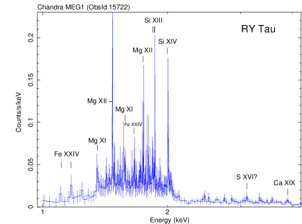
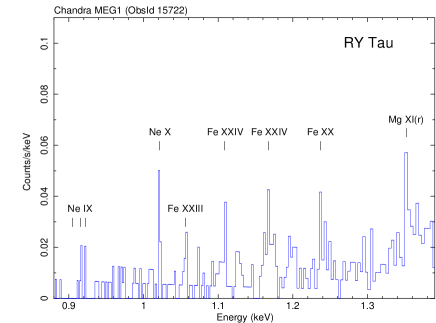
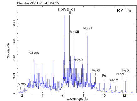
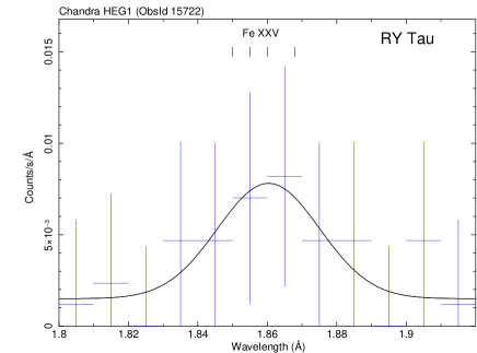
Figure 7: Lightly-binned Chandra 1st-order grating spectra ($+$1 and $-$1 orders combined) of RY Tau for the full ObsId 15722 exposure (85.5 ks). Vertical lines mark reference energies/wavelengths. Top: MEG1 plotted versus energy. Error bars omitted for clarity on low-energy portion at right. Bottom Left: MEG1 plotted versus wavelength. Error bars omitted for clarity.  Bottom Right: HEG1 showing the Fe K$\alpha$ line complex with reference wavelengths of four Fe XXV transitions marked. The fitted Gaussian line width (FWHM = 0.034 Å) is broader than the instrumental width and indicates contributions from multiple Fe XXV lines.

Visible lines at higher energies above 1 keV are Ne X at 1.022 keV (12.134 Å) and Mg XII at 1.47 keV (8.42 Å). The Si XIII triplet near 1.86 keV may also be present but is more clearly detected in the Chandra MEG spectrum (Fig. 7). At low energies below 1 keV background begins to dominate and line identifications become more uncertain. Fe XVII is present and the O VIII line at 0.654 keV (18.97 Å) is also visible in RGS2 but is weak or absent in RGS1. The Ne IX triplet is not detected by RGS2 and there is no RGS1 coverage of Ne IX.

There is a noticeable feature in RGS1 at E = 0.577 $\pm$ 0.002 (1$\sigma$) keV which is slightly higher than the reference energy of the O VII resonance line (E_ref = 0.574 keV). RGS2 lacks coverage at this energy. There is a Ca XVI transition at E_ref = 0.577 keV but RGS1 simulations do not reproduce the Ca line. If the feature is interpreted as O VII then the rather large 3 eV blueshift is not readily explained as a calibration offset or a Doppler shift such as might arise if O VII formed in the blueshifted jet. The latter interpretation would require much higher jet speeds than have been obtained from optical measurements (Sec. 6.4). The identification of this feature as O VII is thus questionable and inspection of the RGS1 background spectrum raises suspicions that it is noise-related.

5.3.2 Chandra HETG

The 1st order MEG spectrum from the longer first observation (ObsId 15722) is shown in Figure 7 along with a portion of the HEG spectrum in the vicinity of the high-temperature Fe K$\alpha$ line complex. Several emission lines are detected (Table 5) superimposed on a hot continuum. The emission lines span a broad range of temperature as judged from maximum line emissivity temperatures of $\sim$6 MK (Ne X) up to $\sim$63 MK (Fe XXV; visible in HEG). There are no high-confidence HETG line detections at energies below 1 keV but weak Ne IX emission may be present near 0.922 keV (13.447 Å ) as discussed further in Sec. 5.4. The absence of strong line detections below 1 keV is attributable to the rapid falloff in ACIS-S/HETG effective area at low energies and the effects of source absorption. We also note that potentially useful Ly$\beta$ lines from O and Ne are not detected so estimates of N_H using Ly$\alpha$/Ly$\beta$ flux ratios are precluded.

The excellent energy resolution and calibration of HETG permit a rigorous comparison of observed line centroid energies with their reference (rest-frame) values and checks for line-broadening. Best-fit first-order MEG line-centroid energies (Table 5) show no significant offsets from the reference energies given in ATOMDB v3.0.2. Gaussian fits of the brightest lines yield centroid energies that differ by at most $\pm$1 eV from reference energies, well within MEG calibration accuracy. Measured line-widths of the brightest lines (Si XIV, Si XIII$r$, Mg XII, Ne X) do not exceed instrumental values. Thus, no evidence for significant centroid shifts or excess line broadening is found for those lines bright enough to confidently measure line properties.

The high plasma temperatures inferred from zero-order ACIS-S fits are confirmed by continuum fits of the MEG spectrum using intervals with no discernible line emission, as determined by visual inspection and the ATOMDB line list. Fits of the MEG spectrum obtained during the first exposure (ObsId 15722) using an absorbed 1T bremsstrahlung model give kT = 8.0 ($+$…,$-$4.3) keV for the high-state interval and kT = 4.4 ($+$8.3,$-$1.9) keV for the subsequent low-state, where the errors are 1$\sigma$. No useful constraint on the upper limit of kT was obtained for the high-state spectrum. Because of the limited number of channels fitted after removing line intervals, no significant improvement was obtained using a 2T bremsstrahlung model. The above values are similar to those obtained from ACIS-S fits using 1T apec models (Table 3).

The 1st order MEG spectrum from the second shorter observation (ObsId 17539) contains only 495 counts as compared to 3796 MEG counts in the first observation. The lower number of counts in the second observation is due to the shorter exposure time and the lower count rate (Fig. 2). Since the spectrum was evolving between the first and second observations we have chosen not to coadd the two MEG spectra. Only the brightest emission lines were detected in the second observation (i.e. Si XIV Ly$\alpha$, Si XIII, Mg XII Ly$\alpha$). The fluxes of these brightest lines are similar in the two observations and their respective 1$\sigma$ confidence flux ranges overlap, albeit with larger flux uncertainties in the second observation due to fewer counts. For the brightest line in the spectrum, Si XIV Ly$\alpha$, the flux from the second observation is F_SiXIV = 8.26 $\pm$ 3.37 (1$\sigma$) $\times$ 10^-6 ph cm^-2 s^-1, in good agreement with the first observation (Table 5).

Table 5: RY Tau Emission Line Properties

Ion	$\lambda_{ref}$	$E_{ref}$	$E_{obs}$	Line Flux (MEG)	Line Flux (RGS)	log $T_{e,max}$
	(Å)	(keV)	(keV)	(10-6 ph cm-2 s-1)	(10-6 ph cm-2 s-1)	(K)
Fe XXV	1.850	6.702	6.664	7.86 $\pm$ 4.52	…	7.8
Ca XIX	3.177	3.903	3.902	3.76 $\pm$ 1.56	…	7.5
Si XIV Ly$\alpha$	6.182	2.006	2.006	8.34 $\pm$ 1.27	…	7.2
Si XIII(r)	6.648	1.865	1.865	4.43 $\pm$ 1.02	…	7.0
Si XIII(i)	6.688	1.854	[1.854]	1.81 $\pm$ 0.80	…	7.0
Si XIII(f)	6.740	1.840	[1.840]	3.55 $\pm$ 0.91	…	7.0
Mg XII	7.106	1.745	1.744	1.73 $\pm$ 0.73	…	7.0
Fe XXIV	7.457	1.663	1.663	1.34 $\pm$ 0.65	…	7.3
Mg XII Ly$\alpha$	8.421	1.472	1.472	5.54 $\pm$ 0.97	5.66 $\pm$ 3.51	7.0
Mg XI(r)	9.169	1.352	1.352	4.02 $\pm$ 1.57	$\leq$3.36	6.8
Mg XI(i)	9.231	1.343	[1.343]	$\leq$1.14	…	6.8
Mg XI(f)	9.314	1.331	[1.331]	$\leq$1.43	…	6.8
Fe XX	10.021	1.237	1.237	1.95 $\pm$ 0.91	…	7.1
Ne X Ly$\beta$	10.239	1.211	[1.211]	$\leq$0.60	…	6.8
Fe XXIV	10.619	1.168	1.167	3.57 $\pm$ 1.12	…	7.3
Fe XXIV	11.176	1.109	1.109	2.05 $\pm$ 0.97	…	7.3
Fe XXIII	11.736	1.056	1.056	2.50 $\pm$ 1.24	…	7.2
Ne X Ly$\alpha$	12.134	1.022	1.021	3.99 $\pm$ 1.73	3.65 $\pm$ 1.72	6.8
Ne IX(r)	13.447	0.922	[0.922]	$\leq$3.65	$\leq$2.44	6.6
Fe XVII	15.014	0.826	[0.826]	$\leq$2.19	1.78 $\pm$ 1.46	6.8
O VIII Ly$\beta$	16.006	0.775	[0.775]	…	$\leq$3.05	6.5
Fe XVII	16.780	0.739	0.736	…	1.59 $\pm$ 1.53	6.8
O VIII Ly$\alpha$	18.969	0.654	0.655	…	2.44 $\pm$ 2.33	6.5
O VII(r)	21.602	0.574	[0.574]	…	$\leq$3.09	6.3

Table 6: RY Tau He-like Triplet Emission Lines

	Si XIII	Mg XI
Grating	HETG (MEG)	HETG (MEG)
Time interval	total	high-state
Flux($r$)	4.43 $\pm$ 1.02	4.02 $\pm$ 1.59
Flux($i$)	1.81 $\pm$ 0.80	$\leq$1.14
flux($f$)	3.55 $\pm$ 0.91	$\leq$1.43
G	1.21${}^{+0.86}_{-0.54}$	$\leq$0.64
R	1.96${}^{+2.46}_{-0.95}$	…
R0	2.3	2.7
log Te,max (K)	7.0	6.8
log Te (K)	6.6${}^{+0.4}_{-0.3}$	$\geq$6.9
log ne (cm-3)	13.0${}^{+0.9}_{-...}$	…

5.4 He-like Triplets

Line emission from He-like triplets is summarized in Table 6. Line flux ratios of the resonance (r), intercombination (i), and forbidden (f) lines of He-like triplets are important plasma diagnostics (Porquet et al. 2001). One or more of the triplet lines of Si XIII and Mg XI is visible in the MEG first order spectrum. Weak emission is also present in MEG at the reference energies of the Ne IX $r$ and $i$ lines, as discusssed further below. The O VII triplet was not detected by MEG and the identification of the feature in RGS1 offset by 3 eV from the O VII$r$ reference energy is uncertain.

In He-like triplets, the line flux ratio $R$ = $f/i$ is sensitive to both electron density $n_{e}$ and the UV radiation field (Gabriel & Jordan 1969). If $\phi$ is the photoexcitation rate from the ³S₁ level to the ³P_2,1 levels, then $R$ = $R_{0}$/[1 $+$ ($\phi$/$\phi_{c}$) $+$ ($n_{e}$/$n_{c}$)], where $\phi_{c}$ and $n_{c}$ are the critical photoexcitation rate and critical density. The quantities $R_{0}$, $\phi_{c}$, and $n_{c}$ depend only on atomic parameters and the electron temperature of the source, as defined in Blumenthal, Drake, & Tucker (1972). For cool stars it is usually assumed that photoexcitation is negligible ($\phi$/$\phi_{c}$ $\approx$ 0), as we do here. However, see Drake (2005) for caveats regarding possible UV effects which can decrease the $R$ ratio, mimicing high densities. The ratio $G$ = ($f+i$)/$r$ is sensitive to electron temperature T_e but is not strongly dependent on $n_{e}$.

The only He-like triplet for which the $r,f$ and $i$ lines were all confidently detected is Si XIII in the MEG spectrum. Si XIII forms in hot plasma at a characteristic temperature T_e,max $\sim$ 10 MK and its $R$ ratio is sensitive only to high densities in the range log $n_{e}$ $\approx$ 13 - 14 (Porquet & Dubau 2000). The computed value $R$ = 1.96${}^{+2.46}_{-0.95}$ based on MEG line fluxes is close to the low-density limit value $R_{0}$ = 2.3 (n_e $<$ n_c), and the two values are consistent within the (large) 1$\sigma$ uncertainties. The computed $R$ ratio formally gives log n_e = 13.0${}^{+0.9}_{-...}$ but since $R$ $\approx$ $R_{0}$ the lower bound on n_e is essentially unconstrained and densities log n_e $<$ 13.0 are allowed.

Although the Mg XI$r$ line was detected in the MEG high-state spectrum, the $i$ and $f$ lines were not. Thus, $R$ is unconstrained for Mg XI but the upper limit on $G$ provides a lower bound log T_e $\geq$ 6.9 (K) which is slightly above the maximum line emissivity temperature log T_e,max = 6.8 (K). The high value of log T_e inferred for Mg XI and the fact that it was only detected by MEG during the high-state (i.e. during the first $\sim$35 ks of ObsId 15722) indicate that it is associated with hot plasma present in the high-state and is unlikely to be shock-related.

The Ne IX triplet is notably absent from the RGS spectrum but a few counts are detected in the lower-background MEG spectrum at the Ne IX$r$ and $i$ reference energies (Fig. 7-top). However, all MEG fits return zero net line flux at the reference energy of Ne IX$f$ so the $f$ line is definitely not detected. The weak Ne IX emission in MEG may contain contributions from Fe XIX and Fe XXI and in any case the emission is too faint to obtain reliable line flux measurements. Thus, we only give an upper limit for Ne IX in Table 5.

5.5 Summary of Spectral Analysis

The X-ray spectrum of RY Tau reveals spectral lines from a broad range of plasma temperature superimposed on a hot continuum. The X-ray spectrum and light curves are highly variable, including short-duration ($\sim$hours) high-temperature flares signaling strong magnetic activity superimposed on slower light curve modulation spanning at least $\sim$one day. The differential emission measure is dominated by very hot plasma with a peak near kT $\approx$ 4 - 5 keV (T $\approx$ 50 MK) and a weaker contribution from cool plasma below 1 keV (T $\,\stackrel{{\scriptstyle\raisebox{-0.60275pt}{$\textstyle<$}}}{{\sim}}\,$ 10 MK). Higher temperatures kT $\sim$ 8 keV (T $\sim$ 90 MK) are inferred during flares. The unabsorbed X-ray luminosity is variable with a typical value log L_x = 30.65 ($\pm$ 0.1) ergs s^-1 outside of flares. The absorption column density N_H is comparable to or perhaps slightly greater than that predicted from A_V. The Fe abundance is significantly subsolar. Undispersed CCD spectra show a faint emission line near 6.4 keV from fluorescent Fe arising in cold material near the star irradiated by the hard X-ray source. No significant line centroid shifts or line broadening were detected for the brightest lines in Chandra MEG spectra. The $R$ ratio computed for the Si XIII He-like triplet is consistent with that expected in the low-density limit. The Mg XI triplet resonance line is only visible in the Chandra MEG spectrum during the high-state when a high plasma temperature was inferred and is thus evidently associated with hot plasma, not shocks. Low-temperature emission lines are generally faint or absent as a result of absorption and RGS noise, although Fe XVII (T_e,max $\sim$ 6 MK) and O VIII Ly$\alpha$ (T_e,max $\sim$ 3 MK) are visible in the RGS spectra.

6 Discussion

6.1 RY Tau in Context: the Taurus CTTS Population

RY Tau is one of the most massive and rapildly-accreting cTTS in Taurus. It is remarkably similar to the prototype T Tau N which dominates the X-ray and optical emission of the multiple T Tau system (Güdel et al. 2007b). RY Tau and T Tau N have similar masses, accretion rates, N_H, and Ne/Fe abundance ratios (Calvet et al. 2004; Güdel et al. 2007b). Both stars have X-ray spectra consisting of an admixture of very hot and very cool plasma with both components exhibiting slow light curve variability (Fig. 2 of Güdel et al. 2007b). The X-ray luminosity of T Tau is log L_x(0.3 - 10 keV) = 31.18 ergs s^-1 (d = 140 kpc), comparable to or slightly greater than that of RY Tau. However, there are a few notable differences. T Tau is a multiple system consisting of at least three closely-spaced objects (T Tau N, T Tau Sa,b) whereas binarity in RY Tau is suspected but has so far not been proven. In addition, no well-collimated large-scale optical jet such as that observed for RY Tau has yet been reported for the T Tau system.

A more quantitative comparison of RY Tau with other cTTS in Taurus can be made using established correlations of L_x with stellar mass (M_∗) and luminosity (L_∗) identified in the XEST cTTS sample (Telleschi et al. 2007a). The correlation with stellar mass is of the form log L_x = $A$$\cdot$log(M_∗/M_⊙) $+$ $B$ (ergs s^-1) where $A$ = 1.70 $\pm$ 0.20 and $B$ = 30.13 $\pm$ 0.09 were determined from the parametric estimation (EM) method and $A$ = 1.98 $\pm$ 0.20 and $B$ = 30.24 $\pm$ 0.06 from the bisector method. We take L_x as the known quantity derived from our X-ray spectral fits and adopt log L_x = 30.65 $\pm$ 0.1 ergs s^-1 (d = 134 pc) as a typical value for RY Tau outside of flares, where the uncertainties reflect only the range of low-state (“quiescent”) L_x values (Tables 3 and 4). Adjusting this value upward to log L_x = 30.69 $\pm$ 0.1 ergs s^-1 at the distance of 140 pc used in the XEST study gives M_∗ = 2.1 (1.8 - 2.7) M_⊙ from the EM-method relation and M_∗ = 1.7 (1.5 - 1.9) M_⊙ from the bisector method, where the range in parentheses accounts only for the uncertainties in XEST regression fit parameters. These mass estimates are in very good agreement with previously published estimates for RY Tau (Table 1). Thus, even though L_x for RY Tau is among the highest of cTTS studied in Taurus (Fig. 1 of Telleschi et al. 2007a), it is consistent with expectations given that its mass is also high.

XEST regression fit results for the EM and bisector methods are similar for the L_x versus L_∗ correlation for cTTS in Taurus, which is log L_x = $C$$\cdot$log(L_∗/L_⊙) $+$ $D$ (ergs s^-1) where $C$ = 1.16 $\pm$ 0.09 and $D$ = 29.83 $\pm$ 0.06. Inserting log L_x = 30.69 for RY Tau yields L_∗ = 5.5 (4.4 - 7.2) L_⊙. This regression fit prediction is a bit lower than previously reported L_∗ values (Table 1) but the upper limit L_∗ = 7.2 L_⊙ is nearly equal to the value 7.6 L_⊙ determined by Kenyon and Hartmann (1995). Given that the spectral type of RY Tau is somewhat uncertain (and hence its bolometric correction as well) and that the low-state (“quiescent”) L_x value is also uncertain by $\pm$0.1 dex, the above difference is not significant. We conclude that published values of M_∗ and L_∗ for RY Tau are in acceptable agreement with predictions based on XEST correlations for cTTS in Taurus.

6.2 The 6.4 keV Fluorescent Fe Line

The 6.4 keV fluorescent Fe emission line is visible in both the EPIC pn and ACIS-S flare or high-state spectra, but is not present in the quiescent or low-state spectra (Figs. 3 and 4). Thus, the fluorescent line is excited by hard X-rays produced in flares or high emission states irradiating cold nearby material. Photon enegies E $>$ 7.11 keV are needed to eject a K-shell electron which is followed by a downward transition (e.g. from the L-shell) to produce the 6.4 keV line. The association of fluorescent Fe emission with flares in young stars and protostars has been seen before, but in unusual cases such as the protostar NGC 2071 IRS1 the 6.4 keV feature is present even in the absence of discernible flares (Skinner et al. 2007; 2009).

Measurements of the continuum-subtracted 6.4 keV line flux in the ACIS-S flare-segment spectrum (ObsId 15722) give F_x,6.4 = 7.5 ($\pm$1.5) $\times$ 10^-14 ergs cm^-2 s^-1, where the uncertainty is 90% confidence. The underlying continuum flux density is F_x,cont = 4.4 ($\pm$0.4) $\times$ 10^-13 ergs cm^-2 s^-1 keV^-1. The above values give a line equivalent width EW = 0.17 $\pm$ 0.05 keV. For comparison, the line flux from the 2003 off-axis ACIS-S spectrum was F_x,6.4 = 4.4 ($\pm$2.0) $\times$ 10^-14 ergs cm^-2 s^-1 (Audard et al. 2005). In our 2013 XMM-Newton observation the EPIC pn 6.4 keV line is narrow and weak and the line flux is quite uncertain but line flux estimates are comparable to that given above for the 2003 Chandra off-axis observation.

The fluorescent line equivalent width (EW) is related to the column density of cold fluorescent material in the optically thin slab approximation by EW $\approx$ 2.3 N₂₄ [keV] (Kallman 1995), where N₂₄ is the column density of the cold matter in units of 10²⁴ cm^-2. Using the value EW = 0.17 $\pm$ 0.05 keV from the 2014 ACIS-S flare spectrum gives N_H,cold = 7.4$\pm$2.2 $\times$ 10²² cm^-2. This value is an order of magnitude greater than inferred from the spectral fits (Table 3) so dense cold target material located near the star but off the line-of-sight is required. Accreting gas or disk gas are two likely possibilities for the irradiated material.

6.3 Slow Variability

The slow decline followed by a slow rise in the Chandra light curves of the first observation is present in very soft, medium, and hard energy bands (Fig. 2). This is a strong clue that the very soft, medium, and hard-band emission have a common origin (Sec. 6.3). Similar slow X-ray light curve variability is present in the shorter second Chandra observation (Fig. 2) and was previously seen in the 2009 Chandra observation (Fig. 2 of SAG11) and the 2003 Chandra off-axis exposure. Furthermore, the EPIC pn light curve in the 1 - 2 keV band on 2013 August 21-22 is rising slowly but no slow variability is obvious in the pn hard-band where rapid flares are most conspicuous (Fig. 1). Taken together, these results suggest that RY Tau is in a persistent state of slow X-ray modulation accompanied by intermittent rapid flares.

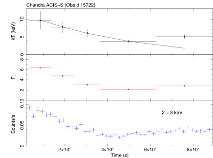
Figure 8: Evolution of mean plasma temperature (kT), absorbed X-ray flux F_x (0.2 - 10 keV; in units of 10^-12 ergs cm^-2 s^-1), and ACIS-S hard-band (2 - 8 keV) count rate versus time for RY Tau during Chandra ObsId 15722. The values of kT and F_x were determined by fitting time-partitioned ACIS-S spectra binned to a minimum of 10 counts per bin using a 1T $apec$ model with metallicity fixed at $Z$ = 0.4 $Z_{\odot}$. The horizontal error bars in the top two panels demarcate the time intervals used to extract time-partitioned spectra. The solid line in the top panel is an exponential fit of the first four data points with an e-folding time of 52.59 ks.

In order to determine how the X-ray parameters changed with time during the slow decay and rise in the new Chandra observation (ObsId 15722), we extracted ACIS-S spectra from five non-overlapping time intervals that span the 85 ks observation. Each spectrum was fitted with an absorbed isothermal 1T $apec$ model with metallicity fixed at $Z$ = 0.4 $Z_{\odot}$. The variation of the mean plasma temperature kT and absorbed broad-band X-ray flux F_x versus time are shown in Figure 8, along with the hard-band ACIS-S light curve.

It is apparent from Figure 8 that kT and F_x declined steadily until the hard-band count rate reached a minimum at elapsed time $t$ $\approx$ 40 - 50 ks and then they increased. The emission measure, as gauged by the XSPEC model $norm$, mimics the time behavior of kT and F_x. An exponential fit of the the kT versus time decay profile (Fig. 8-top) gives an e-folding time of 52.6 ks (14.6 hr).

What is intriguing about the time evolution is that even though kT clearly increased near the end of the observation after the hard-band count rate reached minimum, there is no clear signature of an impulsive flare in the hard-band light curve (Fig. 2) that might have triggered the reheating. Although a slowly-developing flare could be responsible for the gradual brightening after the Chandra light curve reached minimum, the absence of any discernible hard-band flare in combination with the similar slowly-changing count rates in different energy bands is more suggestive of variability associated with one or more surface features rotating across the line-of-sight. The conclusion that the slow light curve variability may be linked to surface structures rotating across the line-of-sight is tentative since no definite stable period of order $\sim$days that could arise from stellar rotation has yet been found in X-rays or optical. However, Holtzman et al. (1986) have presented compelling arguments for surface structures (“spots”) on RY Tau based on their analysis of optical photometric and spectroscopic variability.

Although no definite rotation period for RY Tau has yet been found, a rough estimate can be derived based on published stellar parameters. Estimates of the stellar radius range from R_∗ = 2.9 $\pm$ 0.4 R_⊙ (Calvet et al. 2004) to 5.0 $\pm$ 0.3 R_⊙ (Takami et al. 2013). Petrov et al. (1999) obtained a projected rotational velocity $v$sin$i$ = 52 $\pm$ 2 km s^-1. The disk inclination is quite uncertain with published estimates ranging from $i_{disk}$ = 25^∘ $\pm$ 3^∘ (Akeson et al. 2005) to $i_{disk}$ = 66^∘ $\pm$ 2^∘ (1.3 mm data) or 71^∘ $\pm$ 6^∘ (2.8 mm data), the last two being derived from CARMA mm interferometry (Isella et al. 2010). Based on the above we adopt the representative values R_∗ = 4 $\pm$ 1 R_⊙, $v$sin$i$ = 52 $\pm$ 2 km s^-1 , and $i_{disk}$ = 48^∘ $\pm$ 24^∘. Under the additional assumption that the stellar and disk rotation axes are aligned we obtain P_rot = 2.9 (1.2 - 4.8) days where the range in parentheses reflects the spread in adopted stellar parameters. We emphasize that the above is just an estimate and not a substitute for an observational period determination.

We are not aware of any reports of optical periods of $<$5 days for RY Tau. A slight peak of 5.6 d was noted in a periodogram by Herbst et al. (1987) but after more detailed analysis no significant power near 5.6 d was seen. Later attempts to recover the 5.6 d signal also gave negative results (Herbst & Koret 1988; Bouvier et al. 1993). A low-significance peak of 7.5 d was claimed by Zajtseva (2010) in optical photometry obtained during 1996 but to our knowledge this period has not been confirmed. There have been reports of periods in the range $\sim$20 - 24 d but these are too long to be due to rotation as was noted by Bouvier et al. (1993).

On a rapidly-rotating accreting young star like RY Tau surface structures could originate in coronal active regions or at accretion footpoints, giving rise to X-ray modulation. Periodic X-ray modulation was found in 23 young stars in the Chandra Orion COUP sample (Flaccomio et al. 2005). In most cases the X-ray period was close to the known optical period (P_opt $\sim$2 - 14 d) but in some cases the X-ray period was about half the optical period. Compact sizes less than (or much less than) R_∗ were inferred for the X-ray structures responsible for the modulation. In addition, possible periodic X-ray modulation in the eruptive young star V1647 Ori was attributed to surface structures associated with accretion footpoints (Hamaguchi et al. 2012).

Since the slow Chandra light curve variability is present in very soft and hard energy bands, it is unlikely that the surface structures thought to underlie the variability are accretion footpoints. The predicted accretion shock temperature for RY Tau is T_s $\sim$ 3 MK (Sec. 6.4) and such cool plasma would have little if any effect on the hard-band (2 - 8 keV) light curve. Identification of the presumed surface structures with one or more active regions spanning a range of temperature (and density) seems to be in better accord with the light curve variations. Any role that the hypothesized (but as yet unseen) companion might play in the X-ray variability cannot be reliably assessed without specific information regarding the companion type and its orbit.

The volume V of the X-ray emitting region can be estimated from the volume emission measure EM = n${}_{e}^{2}$V, where n_e is the average electron density in the emitting region. A numerical value of EM is obtained from the XSPEC $norm$ in spectral fits via the relation (Table 3 Notes) EM = 2.15 $\times$ 10⁵⁶ $\times$ $norm$ (cm^-3). In non-flaring states the 1T $apec$ fits give $norm$ $\approx$ (1 - 2.5) $\times$ 10^-3 cm^-5 (Table 3) and as a representative value we adopt $norm$ $\approx$ 1.5 $\times$ 10^-3 cm^-5. This yields EM = 3.2 $\times$ 10⁵³ cm^-3 = n${}_{e}^{2}$V which would include any excess X-ray emission measure from active regions as well as a basal contribution from the ambient corona. As such, it is only an upper limit on any active region contribution. For a stellar radius R_∗ = 2.9 R_⊙ (Calvet et al. 2004) the ratio of emitting region volume to stellar volume is V/V_∗ $\approx$ 0.1/n${}_{e,10}^{2}$ where n_e,10 is the average density in units of 10¹⁰ cm^-3.

Coronal densities in late-type stars determined from O VII and Ne IX triplet line ratios are typically in the range n_e $\sim$ 10¹⁰ - 10¹² cm^-3 (Ness et al. 2004). Active region densities on the Sun obtained from spatially-resolved Hinode observations are in the range n_e $\sim$ 10⁸ - 10¹¹ cm^-3 (Pradeep et al. 2012), being at the high end of this range in the active region core. For an assumed value n_e $\sim$ 10¹⁰ cm^-3 the relation obtained above for RY Tau gives V $\approx$ 0.1V_∗ and a characteristic emitting region radius R = V^1/3 $\approx$ 0.75 R_∗. For a surface filling factor $f$ the relation R = $\sqrt{f}$R_∗ yields $f$ = 0.56. Higher densities are certaintly possible as referenced above and are compatible with the Si XIII triplet line ratios (Table 6), so a small emitting volume V $<$ V_∗ seems assured and the filling factor need not be large.

6.4 Cool Plasma: Shocks or Corona?

The presence of the O VIII Ly$\alpha$ emission line in the RGS2 spectrum supports the conclusion from DEM fits (Fig. 5) that some cool plasma is present. The O VIII line has a maximum emissivity temperature T_e,max $\approx$ 3 MK but the emissivity is still substantial up to higher temperatures of $\sim$5 - 6 MK. Cool plasma at T $\,\stackrel{{\scriptstyle\raisebox{-0.60275pt}{$\textstyle<$}}}{{\sim}}\,$ 3 MK could potentially arise in shocks, and a cool coronal component at T $\sim$3 - 6 MK could also produce the O VIII line.

Shocked Jet: Plasma temperatures of $\sim$3 MK are difficult to achieve for a shocked jet in RY Tau based on current jet speed estimates. As discussed in SAG11, the maximum shock temperature for a shock-heated jet is $T_{s}$ = 0.15$v_{s,100}^{2}$ MK, where $v_{s,100}$ is the jet speed in units of 100 km s^-1 (Raga et al. 2002). The optically-derived jet speed for RY Tau is $v_{jet}$ $\approx$ 165 km s^-1 which leads to a maximum predicted shock temperature $T_{s}$ $\approx$ 0.4 MK (k$T_{s}$ $\approx$ 0.035 keV). At this temperature, almost all of the X-ray emission would emerge at energies below 0.2 keV where XMM-Newton or Chandra have very little sensitivity. Unless the jet speed is higher than estimated from optical observations or other jet-heating mechanisms besides shocks are at work, a jet origin for the cool X-ray plasma is difficult to justify.

Accretion Shock: The case for producing cool (T $\sim$ 3 MK) X-ray plasma and the O VIII line by an accretion shock is more favorable. The post-shock temperature for a strong accretion shock is

$$T_{s}=2.27\times 10^{5}\mu\left[\frac{v_{s}}{100~{}\rm{km~{}s^{-1}}}\right]^{2}~{}K.$$ (1)

where $\mu$ is the mean mass (amu) per particle in the accreting gas and $v_{s}$ is the free-fall speed at the the shock interface (Calvet & Gullbring 1998) To estimate $v_{s}$ we adopt the stellar parameteres of Calvet et al. (2004), namely M_∗ = 2.0 M_⊙, R_∗ = 2.9 R_⊙. The accretion rate is somewhat uncertain but the various models considered by Schegerer et al. (2008) are compatible with rates of $\dot{M}_{acc}$ $\approx$ (2.5 - 9.1) $\times$ 10^-8 M_⊙ yr^-1. We adopt a value in the middle of this range $\dot{M}_{acc}$ = 5 $\times$ 10^-8 M_⊙ yr^-1. In the absence of a magnetic field measurement we assume a typical cTTS value B_∗ $\approx$ 2000 G (Johns-Krull 2007). Using equation (1) of Königl (1991) we obtain an inner disk truncation radius from which the infalling material is assumed to originate of $r_{in}$ = 7.15 R_∗, assuming spherical accretion and H-ionized solar abundance plasma ($\mu$ = 0.6). Equation (1) of Calvet & Gullbring (1998) then gives $v_{s}$ = 479 km s^-1 corresponding to a post-shock temperature T_s = 3.1 MK (kT_s = 0.27 keV). The value of T_s is only weakly-dependent on the poorly-known values B_∗ and $\dot{M}_{acc}$.

For our adopted stellar parameters the post-shock electron density for a strong shock is (eq. [3] of Telleschi et al. (2007b) $n_{2}$ $\approx$ 5.7 $\times$ 10¹⁰${\dot{M}_{acc,-8}}/f$ cm^-3, where $\dot{M}_{acc,-8}$ is in units of 10^-8 M_⊙ yr^-1 and $f$ is the surface filling factor which is not well-known but is usually taken to be in the range $f$ = 0.001 - 0.1. For ${\dot{M}_{acc,-8}}$ = 5 and $f$ $\leq$ 0.1 the lower limit is $n_{2}\raisebox{-2.58334pt}{$\,\stackrel{{\scriptstyle\raisebox{-0.60275pt}{$\textstyle>$}}}{{\sim}}\,$}$ 2.8 $\times$ 10¹² cm^-3. This value is higher than typical coronal densities n_e $\sim$ 10¹⁰ - 10¹¹ cm^-3 for active stars based on O VII triplet $R$ ratios (Ness et al. 2004). The total accretion luminosity is (Calvet & Gullbring 1998) $L_{acc}$ = 3.6 $\times$ 10³³ ergs s^-1 (= 0.94 L_⊙). For comparison, we note that the observed (absorbed) flux of the O VIII Ly$\alpha$ line gives L_OVIII = 4.8 $\times$ 10²⁷ ergs s^-1 with an uncertainty of about a factor of two. The intrinsic (unabsorbed) luminosity depends sensitively on N_H toward the line-forming region and would be larger.

We have fitted the RGS2 spectrum (flares excluded) using a 2T $vapec$ optically thin plasma model to estimate the temperature range needed to reproduce the O VIII Ly$\alpha$ line. Absorption was restricted to the range (4 - 6) $\times$ 10²¹ cm^-2 and the hot plasma component temperature was fixed at kT_hot = 4.35 keV as determined from EPIC pn fits. Subsolar abundances were adopted with Fe = 0.3 and O = 0.3 $\times$ solar. In order to obtain sufficient flux to reproduce the O VIII line, cool component temperatures in the range kT_cool $\approx$ 0.13 - 0.28 keV (T_cool $\approx$ 1.5 - 3.2 MK) are required. These values are consistent with the accretion shock temperature estimated above. Even though accretion shock temperatures are favorable for producing O VIII, the fraction of soft X-rays that could escape and be detected is sensitive to the line-of-sight absorption toward the shock region and photon escape becomes problematic at high infalling gas densities (Drake 2005).

Cool Corona: Coronal plasma in active low-mass stars is distributed over a wide range of temperature and can include both a hot component (T_hot $\,\stackrel{{\scriptstyle\raisebox{-0.60275pt}{$\textstyle>$}}}{{\sim}}\,$ 10 MK) as well as a cool component extending down to temperatures of T_cool $\sim$ 3 - 4 MK. Two examples are the young solar analog EK Dra (Güdel et al. 1997) and the active binary II Peg (Huenemoerder, Canizares, & Schulz 2001), the latter showing a strong coronal O VIII Ly$\alpha$ line.

Electron density information derived from O VII and Ne IX He-like triplets is typically used to discriminate between cool dense plasma in an accretion shock and cool lower-density coronal plasma. In RY Tau the O VII and Ne IX triplets are only weakly detected if at all, so cool plasma density information is lacking. However, as we have noted, the slow variability seen in the Chandra very-soft and medium band light curves mimics that of the hard-band (Fig. 2), providing compelling evidence that some or all of the very soft band emission shares a common origin with the hard-band emission. The hard-band emission is undoubtedly associated with very hot plasma that cannot be reconciled with cool shocks and is thus presumably coronal, but possible contributions from the star-disk magnetic interaction region are not ruled out at the existing limits of X-ray telescope spatial resolution. By association, at least some of the cool plasma must also be of magnetic (non-shock) origin.

7 Summary

We have presented new results clarifying the X-ray properties of the cTTS RT Tau based on observations obtained with Chandra and XMM-Newton. The main results of this study are the following:

1. The X-ray emission of RY Tau is strongly variable, consisting of intermittent rapid flares typical of coronal magnetic activity superimposed on slow light-curve modulation that may be tied to rotation of surface features across the line-of-sight.

2. The absorption column density N_H $\approx$ (4 - 6) $\times$ 10²¹ cm^-2 determined from X-ray spectral fits is comparable to or slightly larger than anticipated from A_V.

3. The characteristic X-ray luminosity of RY Tau log L_x $\approx$ 30.65 ergs s^-1 is among the highest of cTTS in Taurus but is nevertheless consistent with expectations based on its rather high mass and a known correlation between L_x and stellar mass in the Taurus cTTS population.

4. The X-ray emission measure distribution of RY Tau is dominated by hot plasma at characteristic temperatures of kT_hot $\sim$ 4 - 5 keV (T_hot $\sim$ 50 MK), but higher temperatures are recorded during flares. Flares give rise to fluorescent emission from neutral or near-neutral Fe at 6.4 keV arising from irradiated cold dense gas near the star. Gas in the accretion disk or accretion streams provides potential fluorescent target material.

5. A cool plasma component is present which varies slowly in lockstep with hotter plasma, providing a strong clue that at least some of the cool plasma is physically associated with the hotter plasma. Shocks cannot explain the very high temperatures of hot plasma which is undoubtedly associated with magnetic heating processes in the corona or perhaps in the star-disk magnetic interaction region. By association, at least some of the cool plasma is also of magnetic (non-shock) origin.

6. Any contribution to the X-ray emission measure from cool plasma (T_cool $\,\stackrel{{\scriptstyle\raisebox{-0.60275pt}{$\textstyle<$}}}{{\sim}}\,$ 3 MK) originating in the shocked jet or an accretion shock is small compared to the dominant hot plasma, but an accretion shock origin for the O VIII Ly$\alpha$ line is not ruled out.

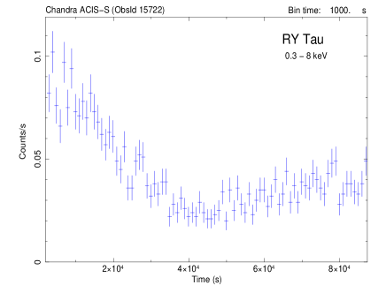
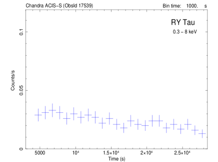
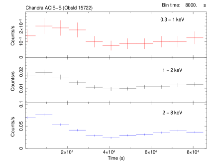
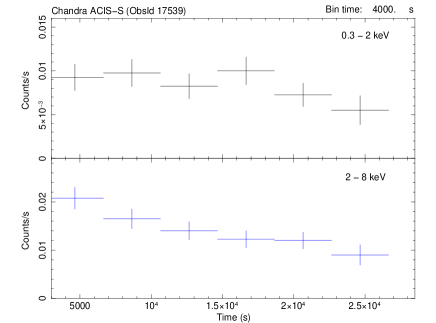
Figure 2: Top: Chandra ACIS-S 0-order light curves (0.3 - 8 keV; 1000 s time bins) of RY Tau for ObsId 15722 (left) and 17539 (right). Times are relative to the observation start time. A gap of $\approx$18.5 hours occurred between the end of the first and beginning of the second observations.  Bottom Left: Chandra ACIS-S 0-order light curves of RY Tau in three different energy bands for ObsId 15722 (8000 s time bins). Similar variability is present in very soft (0.3 - 1 keV), medium (1 - 2 keV), and hard (2 - 8 keV) energy bands.  Bottom Right: Chandra ACIS-S 0-order light curves of RY Tau in the 0.3 - 2 keV and 2 - 8 keV energy bands for ObsId 17539 (4000 s time bins). There are insufficient counts to generate a very soft band (0.3 - 1 keV) light curve.

References

- (1) Agra-Amboage, V., Dougados, C., Cabrit, S., Garcia, P.J.V., & Ferruit, P. 2009, A&A, 493, 1029
- (2) Akeson, R.L. et al. 2005, ApJ, 622, 440
- (3) Anders, E., & Grevesse, N. 1989, Geochim. Cosmochim. Acta, 53, 197
- (4) Audard, M., Skinner, S.L., Smith, K.W., Güdel, M., & Pallavicini, R. 2005, in Proc. 13th Cambridge Workshop on Cool Stars, Stellar Systems, and the Sun, eds. F. Favata et al., ESA SP-560, 411
- (5) Bally, J. Feigelson, E., & Reipurth, B. 2003, ApJ, 584, 843
- (6) Bertout, C., 1989, ARA&A, 27, 351
- (7) Bertout, C., Robichon, N., & Arenou, F. 1999, A&A, 352, 574
- (8) Blumenthal, G.R., Drake, G.W.F., & Tucker, W.H. 1972, ApJ, 172, 205
- (9) Bouvier, J., Cabrit, S., Fernández, M., Martín, E.L., & Matthews, J.M. 1993, A&A, 272, 176
- (10) Brickhouse, N.S., Cranmer, S.R., Dupree, A.K., Luna, G.J.M., & Wolk, S. 2010, ApJ, 710, 1835
- (11) Calvet, N. & Gullbring, E. 1998, ApJ, 509, 802
- (12) Calvet, N., Muzerolle, J., Briceño, C., Hernández, J., Hartmann, L., Saucedo, J.L., & Gordon, K.D. 2004, AJ, 128, 1294
- (13) Drake, J.J. 2005, in Proceedings of the 13th Workshop on Cool Stars, Stellar Systems, and the Sun, ESA SP-560, eds. F. Favata et al., 519
- (14) Favata, F., Bonito, R., Micela, G., Fridlund, M., Orlando, S., Sciortino, S., & Peres, G. 2006, A&A, 450, L17
- (15) Favata, F., Fridlund, C.V.M., Micela, G., Sciortino, S., & Kaas, A.A. 2002, A&A, 386, 204
- (16) Feigelson, E.D. & Montmerle, T., 1999, ARA&A, 37, 363
- (17) Flaccomio, E., Micela, G., Sciortino, S., Feigelson, E.D., Herbst, W., Favata, F., Harnden, F.R., & Vrtilek, S.D. 2005, ApJS, 160, 450
- (18) Gabriel, A.H. & Jordan, C. 1969, MNRAS, 145, 241
- (19) Glassgold, A.E., Najita, J., & Igea, J., 1997, ApJ, 480, 344
- (20) Gómez de Castro, A.I. & Verdugo, E. 2007, ApJ, 654, L91
- (21) Gorenstein, P., 1975, ApJ, 198, 95
- (22) Grosso, N., Feigelson, E.D., Getman, K.V., Kastner, J.H., Bally, J., & McCaughrean, M.J. 2006, A&A, 448, L29
- (23) Güdel, M. et al. 2007a, A&A, 468, 353
- (24) Güdel, M., Guinan, E.F., Mewe, R., Kaastra, J.S., & Skinner, S.L. 1997, ApJ, 479, 416
- (25) Güdel, M., Skinner, S.L., Briggs, K.R., Audard, M., Arzner, K., & Telleschi, A., 2005, ApJ, 626, L53
- (26) Güdel, M., Skinner, S.L., Audard, M., Briggs, K., & Cabrit, S. 2008, A&A, 478, 797
- (27) Güdel, M., Skinner, S.L., Mel’nikov, S.Y., Audard, M., Telleschi, A., & Briggs, K.R., 2007b, A&A, 468, 529
- (28) Hamaguchi, K. et al. 2012, ApJ, 754, 32
- (29) Herbst, W. et al. 1987, AJ, 94, 137
- (30) Herbst, W. & Koret, D.L. 1988, AJ, 96, 1949
- (31) Holtzman, J.A., Herbst, W., & Booth, J. 1986, AJ, 92, 1387
- (32) Huenemoerder, D.P., Canizares, C.R., & Schulz, N.S. 2001, ApJ, 559, 1135
- (33) Ismailov, N.Z. & Adygezalzade, A.N. 2012, Ast. Reports, 56, 131
- (34) Isella, A., Carpenter, J.M., & Sargent, A.I. 2010, ApJ, 714, 1746
- (35) Johns-Krull, C.M. 2007, ApJ, 664, 975
- (36) Judge, P.G. & McIntosh, S.W. 1999, Sol. Phys., 190, 331
- (37) Kallman, T.R., 1995, ApJ, 455, 603
- (38) Kastner, J.H., Huenemoerder, D.P., Schulz, N.S., Canizares, C.R., & Weintraub, D.A. 2002, ApJ, 567, 434
- (39) Kenyon, S.J. & Hartmann, L. 1995, ApJS, 101, 117
- (40) Königl, A. 1991, ApJ, 370, L39
- (41) Leinert, Ch., Zinnecker, H., Weitzel, N., Christou, J., Ridgway, S.T., Jameson, R., Haas, M., & Lenzen, R. 1993, A&A, 278, 129
- (42) Ness, J.-U., Güdel, M., Schmitt, J.H.M.M., Audard, M., & Telleschi, A. 2004, A&A, 427, 667
- (43) Petrov, P.P., Zajtseva, G.V., Efimov, Y.S., Duemmler, R., Ilyin, I.V., Tuominen, I., & Shcherbakov, V.A. 1999, A&A, 341, 553
- (44) Porquet, D. & Dubau, J. 2000, A&A Supp., 143, 495
- (45) Porquet, D., Mewe, R., Dubau, J., Raassen, A.J.J., & Kaastra, J.S. 2001, A&A, 376, 1113
- (46) Pott, J.-U., Perrin, M.D., Furlan, E., Ghez, A.M., Herbst, T.M., & Metchev, S. 2010, ApJ, 710, 265
- (47) Pradeep, K., Bhupendra, S., & Anil, K. 2012, Res. J. of Recent Sci., 1, 40
- (48) Pravdo, S.H., Feigelson, E.D., Garmire, G., Maeda, Y., Tsuboi, Y., & Bally, J. 2001, Nature, 413, 708
- (49) Pravdo, S.H., Tsuboi, Y., & Maeda, Y. 2004, ApJ, 605, 259
- (50) Raga, A.C., Noriega-Crespo, A., & Velázquez, P.F. 2002, ApJ, 576, L149
- (51) Schegerer, A.A., Wolf, S., Ratzka, Th., & Leinert, Ch. 2008, A&A, 478, 779
- (52) Shang, H., Glassgold, A.E., Shu, F.H., & Lizano, S., 2002, ApJ, 564, 853
- (53) Skinner, S.L., Audard, M., & Güdel, M. 2011, ApJ, 737, 19 (SAG11)
- (54) Skinner, S.L. & Güdel, M. 2014, ApJ, 788, 101
- (55) Skinner, S.L., Simmons, A.E., Audard, M., & Güdel, M. 2007, ApJ, 658, 1144
- (56) Skinner, S.L., Sokal, K.R., Megeath, S.T., Güdel, M., Audard, M., Flaherty, K.M., Meyer, M.R., & Daminelli, A. 2009, ApJ, 701, 710
- (57) Stelzer, B., Hubrig, S., Orlando, S., Micela, G., Mikulás̆ek, Z., & Schöller, M. 2009, A&A, 499, 529
- (58) Stelzer, B. & Schmitt, J.H.M.M. 2004, A&A, 418, 687
- (59) St.-Onge, G. & Bastien, P. 2008, ApJ, 674, 1032
- (60) Takami, M. et al. 2013, ApJ, 772, 145
- (61) Telleschi, A., Güdel, M., Briggs, K.R., Audard, M., & Palla, F. 2007a, A&A, 468, 425
- (62) Telleschi, A., Güdel, M., Briggs, K.R., Audard, M., & Scelsi, L. 2007b, A&A, 468, 443
- (63) Turner, M.J.L. et al. 2001, A&A, 365, L27
- (64) Vuong, M.H., Montmerle, T., Grosso, N., Feigelson, E.D., Verstraete, L., & Ozawa, H. 2003, A&A, 408, 581
- (65) Zajtseva, G.V. 2010, Astrophys., 53 (no. 2), 212