Dynamics of two coupled semiconductor spin qubits in a noisy environment

Abstract

We theoretically consider the temporal dynamics of two coupled spin qubits (e.g., semiconductor quantum dots) driven by the inter-qubit spin-spin coupling. The presence of environmental noise (e.g., charge traps, nuclear spins, random magnetic impurities) is accounted for by including random magnetic field and random inter-qubit coupling terms in the Hamiltonian. Both Heisenberg coupling and Ising coupling between the spin qubits are considered, corresponding respectively to exchange and capacitive gates as appropriate for single spin and singlet-triplet semiconductor qubit systems, respectively. Both exchange (Heisenberg) and capacitive (Ising) coupling situations can be solved numerically exactly even in the presence of noise, leading to the key findings that (i) the steady-state return probability to the initial state remains close to unity in the presence of strong noise for many, but not all, starting spin configurations, and (ii) the return probability as a function of time is oscillatory with a characteristic noise-controlled decay toward the steady-state value. We also provide results for the magnetization dynamics of the coupled two-qubit system. Our predicted dynamics can be directly tested in the already existing semiconductor spin qubit setups providing insight into their coherent interaction dynamics. Retention of the initial state spin memory even in the presence of strong environmental noise has important implications for quantum computation using spin qubits.

I Introduction

Universal quantum computation depends on controllable (and highly accurate) one- and two-qubit gate operations using a suitable physical system of two-level quantum objects (i.e., the qubits). Among the many different physical qubit systems being studied worldwide (e.g., ion traps, neutral atoms, superconducting qubits, spin qubits), both involving atomic and solid-state architectures, semiconductor nanostructure-based spin qubits are perhaps unique in terms of their easy controllability and fast gate operations, and most importantly, in terms of their potential for scalability because of existing semiconductor-based microelectronics technology R1 . The subject of semiconductor spin qubits, which for our purposes in the current work are localized electron spins in semiconductor nanostructures acting as quantum two-level systems, is currently one of the most active research areas in quantum information processing using solid-state materials. In fact, both Si- and GaAs-based spin qubit architectures are being extensively studied in many laboratories all over the world with several breakthrough experiments being reported during the last five or so yearsR2 ; R3 ; R4 ; R5 ; R6 ; R7 ; R8 ; R9 ; R10 ; R11 . In particular, experimental two-qubit systems using localized electron spins have recently been reported for both GaAs and Si nanostructuresR12 ; R13 ; R14 , although the fidelity for such two-qubit gate operations is still rather low due to environmental noise and weak inter-qubit coupling.

The current theoretical work is specifically on a two-qubit system of localized electron spins in semiconductor nanostructures (e.g., Si or GaAs quantum dots, P or other donor states in Si, Si MOS-based qubits, Si-Ge heterostructure-based qubits) with the goal being to understand the quantum dynamics of the two-qubit system in the presence of both inter-qubit coupling and environmental noise. The environmental noise could arise from a number of physical mechanisms, but the most important ones for semiconductor spin qubits are known to be Overhauser noise due to the background nuclear spins and charge noise due to traps and defects in the system. The noise is represented in the theory by a random magnetic field acting on single qubits (i.e., each spin) and a random fluctuation in the two-spin coupling (i.e., the two-qubit interaction). The goal is to understand the behavior of coupled-qubit spin dynamics in the presence of both inter-qubit interaction and environmental noise.

Our theory is primarily motivated by the fact that there are very few laboratory demonstrations of controlled two-qubit coupling in semiconductor spin quantum computing experiments. Even the few that existR12 ; R13 ; R14 typically manifest very poor fidelity and sometimes even poor reproducibilityR15 . This is in sharp contrast with the competing quantum computing architectures involving superconducting and ion trap qubits, where multi-qubit coherent quantum control operations are now routinely achieved in many laboratories with high ($>95\%$) fidelity and reproducibility. Since eventual large-scale quantum information processing would require efficient and controllable one- and two-qubit gates with very high ($>99.9\%$) fidelity, the paucity of two-qubit gate operations in semiconductor spin quantum computing systems is particularly worrisome, and is now universally considered to be the key roadblock for future progress in the field of semiconductor-based quantum computation.

Given the above context of the critical absence of two-qubit coupling demonstration experiments in semiconductor spin quantum computing architectures, it is perhaps imperative to take a step back and consider situations where the two-qubit entanglement dynamics can be directly explored without the complication of gate control operations in order to understand the interplay between qubit coupling and qubit noise. In the current work, therefore, we study theoretically the coupled qubit dynamics of two localized electron spin qubits in semiconductor nanostructures in the presence of finite qubit coupling and finite noise. The theoretical problem allows for an almost exact analytical solution, making the results tractable and leading to specific predictions which are directly testable in the currently existing experimental spin qubit systems. We believe that the experimental demonstration of the theoretical two-qubit coupling dynamics of the current work would be easier than the full two-qubit gate control experiments, providing useful insight into the interplay between interaction and noise in the dynamics of coupled spin qubits. This is because a two-qubit gate control experiment would not only require multiple measurements of return probabilities, one for each member of a suitable orthogonal basis, e.g., $\ket{\uparrow\uparrow}$, $\ket{\uparrow\downarrow}$, $\ket{\downarrow\uparrow}$, and $\ket{\downarrow\downarrow}$, but also requires a means of error correction, which can result in complicated pulse sequences. On the other hand, demonstrating the results of our work simply requires a single measurement of the return probability, and does not require any error correction scheme—one simply lets the system evolve as it will under the influence of both an intentionally applied gate voltage and the noise in the system. Another key difference between performing a quantum computing gate operation and our proposal is that performing a gate operation requires precise control over the timing and duration of pulses, whereas our proposal only involves a simple evolution in time with constant “always on” gate voltages, which is convenient for an experimentalist.

Experimentally, semiconductor spin qubits form essentially a $2\times 2$ matrix in laboratory implementations with both Si and GaAs being used as the materials platform and there being two distinct types of qubit architectures and coupling, namely, the so-called exchangeLossPRA1998 ; DiVincenzoNature2000 ; HuPRA2000 ; ScarolaPRA2005 and capacitiveCalderonVargasPRB2015 ; SrinivasaPRB2015 two-qubit gates, in operation. The two-qubit exchange gate involves a direct Heisenberg coupling between two localized electron spins whereas the two-qubit capacitive gate involves a dipolar capacitive Ising-type coupling between two quantum dot based singlet-triplet qubitsLevyPRL2002 ; PettaScience2005 . We refer to these couplings as Heisenberg (i.e., exchange) and Ising (i.e., capacitive) throughout this paper, and we consider them on an equal footing although their experimental implementations involve different physics and architectures.

In addition to the interqubit coupling, the qubits are affected by environmental noise arising from several different mechanismsHuPRL ; WitzelPRL ; CywinskiPRL ; BarnesPRL ; CywinskiPRB that we parametrize in our theory by random local magnetic fields acting on both qubits (in addition, of course, to any known applied field for qubit control). We also include a noise term in the qubit coupling itself so that the theory has both one- and two-qubit noise. There has been previous work considering magnetic noiseCoishPRB2005 ; KlauserPRB2006 , as well as some limited work on charge noiseKlauserPRB2006 ; however, the latter does not explore the effects of charge noise on the detailed dynamics of the system, and thus we undertake such an investigation here. In particular, the goal of our work is to directly motivate experimental investigations of coupled two-qubit dynamics in recently realized experimental systemsR2 ; R3 ; R4 ; R5 ; R6 ; R7 ; R8 . The main point of the paper is the interplay between the qubit coupling and the qubit noise (both one- and two-qubit) on the temporal dynamics of the coupled qubits, which can be solved essentially analytically, leading to precise experimentally observable consequences. These experiments to verify our predicted coupled qubit dynamics can be performed right now, both for Heisenberg and Ising coupling gates and both in Si and GaAs spin qubit platforms—the necessary laboratory systems for carrying out the qubit dynamics experiments already exist. The experimental situation to be used here is what is commonly referred to as the “always on” configuration, in which the inter-qubit coupling is not turned off at all after it has been turned on.

In Sec. II we review the Heisenberg and Ising models and their diagonalization. In Secs. III and IV, respectively, we provide our (analytical and numerical) results for the Heisenberg and Ising qubit couplings. We conclude in Sec. V with a summary and outlook.

II Models

Below, we review the theoretical models for Heisenberg (Sec. II A) and Ising (Sec. II B) interqubit coupling on an equal footing using the same notation as much as possible, as well as the eigenvalues and eigenvectors for the Heisenberg caseCoishPRB2005 ; KlauserPRB2006 . We review the corresponding results for the Ising caseWangNPJQE in the Appendix. Throughout this paper, we will be working in units in which $\hbar=1$.

II.1 Heisenberg

The Heisenberg Hamiltonian describing two coupled spin qubits in the presence of qubit noise is given by the following disordered Heisenberg Hamiltonian model:

$$H=J\vec{S}_{1}\cdot\vec{S}_{2}+h_{1}S_{1z}+h_{2}S_{2z},$$ (1)

where the sites, $1$ and $2$, denote the two localized electron spins (i.e., qubits) with an interqubit coupling strength $J$ that could have a small random component $\delta J$ in it denoting the noise-induced fluctuation in the interqubit coupling. The quantities, $h_{1}$ and $h_{2}$, are the environmental noise-induced random magnetic fields at the two qubits. In principle, we could add a constant non-random externally applied uniform magnetic field $h_{0}$ to Eq. (1) by redefining $h_{1}\to h_{0}+h_{1}$ and $h_{2}\to h_{0}+h_{2}$, but, as will become clear below, this will have no effect on the dynamics that we describe in this work, and is therefore left out (the situation is different for the Ising model, in which such an external magnetic field will affect the dynamics, making the Ising problem, to be discussed below in Sec. II B, richer and more complex than the Heisenberg case). These noise-induced local magnetic fields, arising from background nuclei and charge noise (and possibly from other unknown sources), are taken to be Gaussian random variables (with no loss of generality—other choices for the random noise distribution do not change any of our conclusions). We assume the noise to be static since it is slow in reality (and its exact time dependence is unknown), but we discuss later in the paper the considerations for dynamic noise.

We note that the total spin $S_{z}=S_{1z}+S_{2z}$ for the two-spin system is conserved and focus on the $S_{z}=0$ subspace, which consists of only two states $\ket{\uparrow\downarrow}$ and $\ket{\downarrow\uparrow}$, where the arrows indicate the $z$ component of the spin (up or down) for each qubit. The reason for restricting ourselves to $S_{z}=0$ is that the other two possibilities, $S_{z}=\pm 1$ (for a two-spin Heisenberg system, there are only three possible $S_{z}$ subspaces, defined by $S_{z}=0,\pm 1$), are trivial since the system is now stuck in a single eigenstate with no dynamics whatsoever.

In the $S_{z}=0$ basis, we can rewrite the two-qubit Hamiltonian asCoishPRB2005 ; KlauserPRB2006

$$H=\tfrac{1}{2}J\sigma_{z}+\tfrac{1}{2}\delta h\sigma_{x}-\tfrac{1}{4}J,$$ (2)

where $\sigma_{x}$ and $\sigma_{z}$ are the usual $2\times 2$ Pauli spin matrices in the $S_{z}$ basis and $\delta h$ is the noise-induced random field difference between qubits $1$ and $2$:

$$\delta h=h_{1}-h_{2}.$$ (3)

We note that $J$ by itself may include a random term $\delta J$ as well. Note that any constant uniform applied magnetic field drops out of $\delta h$ leaving only the noise-induced random field difference between the two qubits (this simplification does not exist for the Ising case as we will see later). Here, we use the convention that the upper component of the wave function corresponds to $\ket{\uparrow\downarrow}$.

The eigenvalue problem for the Hamiltonian defined in Eq. (2) is exactly solvableCoishPRB2005 ; KlauserPRB2006 , giving the following energy eigenvalues $E_{\pm}$ and eigenstates $\psi_{\pm}$:

$$E_{\pm}=-\tfrac{1}{4}J\pm\tfrac{1}{2}\sqrt{J^{2}+(\delta h)^{2}}$$ (4)

and

$$\psi_{\pm}=\begin{bmatrix}\frac{1}{\sqrt{2}}\sqrt{1\pm\frac{\delta h}{\sqrt{J^{2}+(\delta h)^{2}}}}\\ \pm\frac{1}{\sqrt{2}}\sqrt{1\mp\frac{\delta h}{\sqrt{J^{2}+(\delta h)^{2}}}}\end{bmatrix}.$$ (5)

We use these equations to obtain the results presented in Sec. III.

II.2 Ising

The Ising Hamiltonian describing two coupled spin qubits (e.g., singlet-triplet quantum dot qubits) in the presence of qubit noise is given by

$$H=\varepsilon J_{1}J_{2}\sigma_{1}^{z}\sigma_{2}^{z}+J_{1}\sigma_{1}^{z}+J_{2}\sigma_{2}^{z}+h_{1}\sigma_{1}^{x}+h_{2}\sigma_{2}^{x},$$ (6)

where we have expressed the coupled Hamiltonian in the so-called “singlet-triplet basis,” with $\sigma_{1}^{z}=\pm 1$ for the singlet/triplet state of the qubit. In Eq. (6), $J_{i}$ ($i=1,2$) is the individual exchange coupling within the $i$th qubit (usually a two-quantum dot structure) producing the singlet-triplet single qubit (which necessitates an intra-qubit exchange coupling in order to create singlet and triplet levels—this exchange coupling is not the interqubit coupling here, it is merely a parameter defining the qubit itself) whereas the interqubit coupling is given by $\varepsilon J_{1}J_{2}$ with $\varepsilon$ denoting the interqubit coupling strength. The noise-induced random magnetic fields $h_{i}$ ($i=1,2$) act on each qubit by coupling through $\sigma_{i}^{x}$ in the singlet-triplet basis.

Comparing Eq. (6) with Eq. (2), we note significant differences between the Ising and Heisenberg models, with the Ising model being much more complex. In particular, the Ising Hamiltonian, Eq. (6), is a $4\times 4$ matrix in the singlet-triplet basis whereas the Heisenberg Hamiltonian, Eq. (1) or (2), is simply an (effective) $2\times 2$ matrix. One consequence of the richer structure of the Ising coupling (and the associated singlet-triplet semiconductor spin qubits) is that the total (effective) $S_{z}$ is not conserved, in contrast with the Heisenberg coupling, and therefore the Ising Hamiltonian cannot be expressed in a block diagonal form [i.e., $\sigma_{i}^{x}$ and $\sigma_{i}^{z}$ both appear in Eq. (6)] in contrast to the Heisenberg Hamiltonian, which is readily expressed in a block diagonal form in the conserved $S_{z}$ basis. The more complicated nature of the capacitive Ising coupling for the singlet-triplet qubits is also reflected in the larger ($3$) number of parameters ($J_{1}$, $J_{2}$, $\varepsilon$) necessary to define the qubit Hamiltonian compared with the Heisenberg Hamiltonian, for which the simple exchange coupling between the two spins is described by just one parameter, the Heisenberg exchange coupling $J$.

It turns out, however, that in spite of the complicated nature of the Ising Hamiltonian, one can still diagonalize it analytically, leading to an explicit construction of the time evolution operator controlling the qubit dynamics. Unfortunately, this analytical solution is built upon the roots of a quartic equationWangNPJQE and does not have an easily transparent (or manageable) form for actual calculations. We therefore review this analytical solution in the Appendix of the current paper.

We note that in general one can think of the random on-site magnetic field disorder to be arising from the nuclear Overhauser noise and the noise in the exchange coupling itself to be arising from the charge noise. This qualitative distinction between Overhauser and charge noise applies to both Heisenberg and Ising coupling situations.

III Heisenberg coupling

We first present our detailed results for the Heisenberg Hamiltonian, Eqs. (1) and (2). We will consider two starting states—the “classical” state, $\ket{\uparrow\downarrow}$, and the singlet state, $\ket{S}=\frac{1}{\sqrt{2}}(\ket{\uparrow\downarrow}-\ket{\downarrow\uparrow})$. Results for the qubit dynamics depend strongly on the initial state.

III.1 “Classical” starting state

We start by giving the return probability and the magnetization at each site, with “magnetization” here simply meaning the expectation value of the spin at the given site. Taking our initial state to be $\ket{\psi(0)}=\ket{\uparrow\downarrow}$, we find that the state at time $t$, $\ket{\psi(t)}$, is

$$\ket{\psi(t)} = \frac{1}{\sqrt{2}}\sqrt{1+\frac{\delta h}{\sqrt{J^{2}+(\delta h)^{2}}}}e^{-iE_{+}t}\ket{+}$$ (7)

$$+ \frac{1}{\sqrt{2}}\sqrt{1-\frac{\delta h}{\sqrt{J^{2}+(\delta h)^{2}}}}e^{-iE_{-}t}\ket{-},$$ (8)

where $\ket{+}$ and $\ket{-}$ are the positive- and negative-energy eigenstates within the $S_{z}=0$ basis, respectively. We then recover the expression for the return probability found in Ref. CoishPRB2005, :

$$P_{\uparrow\downarrow}(t) = \left|\braket{\psi(t)}{\psi(0)}\right|^{2}$$ (9)

$$= 1-\frac{J^{2}}{J^{2}+(\delta h)^{2}}\sin^{2}\left[\tfrac{1}{2}\sqrt{J^{2}+(\delta h)^{2}}t\right]$$ (10)

and the $z$ component of the magnetization of spin $1$ is

$$\braket{S_{1z}(t)} = \braket{\psi(t)}{S_{1z}}{\psi(t)}=\tfrac{1}{2}\left\{\frac{(\delta h)^{2}}{J^{2}+(\delta h)^{2}}\right.$$

$$+ \left.\frac{J^{2}}{J^{2}+(\delta h)^{2}}\cos\left[\sqrt{J^{2}+(\delta h)^{2}}t\right]\right\}.$$

The magnetization of spin $2$ is just $\braket{S_{2z}(t)}=-\braket{S_{1z}(t)}$. We provide plots of the return probability and magnetization for several values of $\delta h$ in Fig. 1.

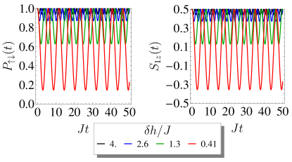
Figure 1: Plot of the return probability, $P_{\uparrow\downarrow}(t)$ (left), and of the magnetization of spin $1$, $\braket{S_{1z}(t)}$ (right), as a function of time for several values of $\delta h$ with the initial state $\ket{\psi(0)}=\ket{\uparrow\downarrow}$.

We now determine the disorder-averaged return probability. We will consider both cases with only magnetic disorder, i.e., disorder in the magnetic fields $h_{1}$ and $h_{2}$, and cases with exchange disorder as well, i.e., disorder in the exchange coupling $J$. We will assume that the magnetic fields both follow a Gaussian distribution with zero mean and standard deviation $\sigma_{h}$; we will refer to the latter as the “strength” of the magnetic disorder. Similarly, we will assume that the exchange coupling follows a truncated Gaussian distribution, restricted to non-negative values, with mean $J_{0}$ and standard deviation, or strength, $\sigma_{J}$. Since the return probability and magnetization only depend on $\delta h$, we may simplify this calculation by noting that $\delta h$ also follows a Gaussian distribution, with zero mean and standard deviation $\sigma_{h}\sqrt{2}$. Results for the cases in which there is a large magnetic field gradient present (i.e., the average field gradient $\delta h_{0}\gg\sigma_{h}$) and in which the exchange coupling is very large (i.e., $J\gg\delta h_{0}$ and $\sigma_{h}$), both with $\sigma_{J}=0$, have been previously found in Ref. KlauserPRB2006, .

The disorder average of some quantity $A$ is given by

$$\left[A\right]_{\alpha}=\int_{0}^{\infty}\,\int_{-\infty}^{\infty}dJ\,d(\delta h)\,f_{\delta h}(\delta h)f_{J}(J)A,$$ (13)

where the probability density $f_{\delta h}(\delta h)$ is given by

$$f_{\delta h}(\delta h)=\frac{1}{2\sigma_{h}\sqrt{\pi}}e^{-(\delta h)^{2}/4\sigma_{h}^{2}}$$ (14)

and $f_{J}(J)$ is given by

$$f_{J}(J)=\frac{1}{\sigma_{J}\sqrt{2\pi}}\frac{2}{1+\mbox{erf}\left(\frac{J_{0}}{\sigma_{J}\sqrt{2}}\right)}e^{-(J-J_{0})^{2}/2\sigma_{J}^{2}}.$$ (15)

This integral must be determined numerically. Using Eqs. (10) and (LABEL:Eq:Mag1_UD), we evaluate this integral for the return probability and the magnetization of spin $1$, respectively, for several values of $\sigma_{h}$ and $\sigma_{J}$ and present the results in Figs. 2 and 3. We see that the return probability and the magnetization oscillate around, and decay to, a steady-state value. We may argue that the period of the oscillations is of order $1/J_{0}$ by noting that the probability distributions for the magnetic and exchange disorder, Eqs. (14) and (15), are peaked at $0$ and $J_{0}$, respectively, and that the oscillation frequency of the oscillatory terms in the single-realization results given in Eqs. (10) and (LABEL:Eq:Mag1_UD) is $\sqrt{J^{2}+(\delta h)^{2}}$. Therefore, contributions to the disorder average of frequency $J_{0}$ will dominate the disorder average. We also note that the decay rate is set by the disorder strengths $\sigma_{h}$ and $\sigma_{J}$, increasing as we increase them. The magnetic disorder strength, in addition, sets the steady-state value; we note that this steady-state value increases as we increase $\sigma_{h}$. The exchange disorder strength also has a small effect, but it is very small compared to the effect of magnetic disorder.

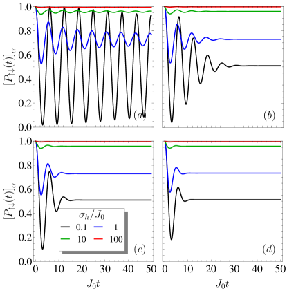
Figure 2: Plot of the disorder-averaged return probability, $\left[P_{\uparrow\downarrow}(t)\right]_{\alpha}$, as a function of time for different values of $\sigma_{h}$, as indicated in the plot, with the initial state $\ket{\psi(0)}=\ket{\uparrow\downarrow}$, for (a) $\sigma_{J}=0$, (b) $\sigma_{J}=0.1J_{0}$, (c) $\sigma_{J}=0.2J_{0}$, (d) $\sigma_{J}=0.3J_{0}$.

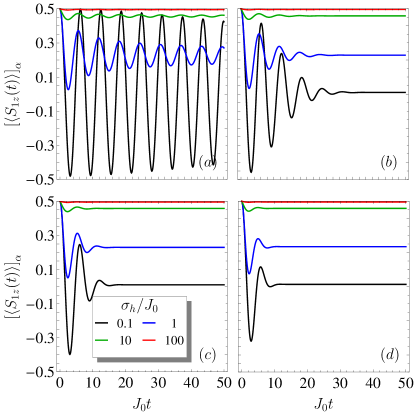
Figure 3: Plot of the disorder-averaged magnetization of spin $1$, $\left[\braket{S_{1z}(t)}\right]_{\alpha}$, as a function of time for different values of $\sigma_{h}$, as indicated in the plot, with the initial state $\ket{\psi(0)}=\ket{\uparrow\downarrow}$, for (a) $\sigma_{J}=0$, (b) $\sigma_{J}=0.1J_{0}$, (c) $\sigma_{J}=0.2J_{0}$, (d) $\sigma_{J}=0.3J_{0}$.

We determine the steady-state values as a function of $\sigma_{h}$ and for $\sigma_{J}=0$ and plot them in Fig. 4. We have also done calculations for $\sigma_{J}\neq 0$, and have verified that the results do not differ significantly from the $\sigma_{J}=0$ results. We also confirm that, for sufficiently large values of $\sigma_{h}$, there is an increase in the steady-state values of the return probability and the magnetization of spin $1$, as noted above. This indicates that strong magnetic disorder helps to preserve the state of the two-qubit system, with the crossover into this behavior happening for $\sigma_{h}$ on the order of $J_{0}$. Of course, in the situation in which the disorder is much larger than the exchange coupling ($\sigma_{h}\gg J_{0}$), this result is trivial since the interqubit interaction is simply unable to flip the initial spins, but as emphasized elsewhere for multiqubit systemsBarnesPRB2016 , the return probability is finite even in the situation when the disorder is not much larger than the coupling, which is neither an intuitive nor an obvious result, and thus should be confirmed experimentally.

Figure 4: Plot of the steady-state disorder-averaged return probability, $\left[P_{\uparrow\downarrow}(t\to\infty)\right]_{\alpha}$ (left), and magnetization of spin $1$, $\left[\braket{S_{1z}(t\to\infty)}\right]_{\alpha}$ (right), as functions of $\sigma_{h}$ for $\sigma_{J}=0$ with the initial state $\ket{\psi(0)}=\ket{\uparrow\downarrow}$.

We should emphasize, however, that, while exchange disorder has only a small effect on the steady-state return probability, it has a significant effect on the dynamics. To this end, we present some of our plots of the return probability and magnetization of spin $1$ in an alternate fashion, in which we fix $\sigma_{h}/J_{0}$ and vary $\sigma_{J}/J_{0}$, in Figs. 5 and 6. We note that changing $\sigma_{J}/J_{0}$ has a large effect on how rapidly the oscillations in these quantities decay.

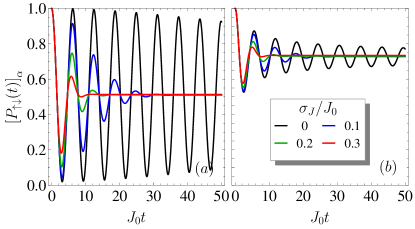
Figure 5: Plot of the disorder-averaged return probability, $\left[P_{\uparrow\downarrow}(t)\right]_{\alpha}$, as a function of time for different values of $\sigma_{J}$, as indicated in the plot, with the initial state $\ket{\psi(0)}=\ket{\uparrow\downarrow}$, for (a) $\sigma_{h}=0.1J_{0}$, (b) $\sigma_{h}=J_{0}$.

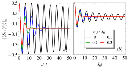
Figure 6: Plot of the disorder-averaged magnetization of spin $1$, $\left[\braket{S_{1z}(t)}\right]_{\alpha}$, as a function of time for different values of $\sigma_{J}$, as indicated in the plot, with the initial state $\ket{\psi(0)}=\ket{\uparrow\downarrow}$, for (a) $\sigma_{h}=0.1J_{0}$, (b) $\sigma_{h}=J_{0}$.

III.2 Singlet starting state

We now consider the same analysis done above, but taking the “singlet” state $\ket{\psi(0)}=\ket{S}=\frac{1}{\sqrt{2}}(\ket{\uparrow\downarrow}-\ket{\downarrow\uparrow})$ as our initial state. In this case, the time-evolved state is given by

$$\ket{\psi(t)} = \tfrac{1}{2}\left[\sqrt{1+\frac{\delta h}{\sqrt{J^{2}+(\delta h)^{2}}}}\right.$$ (16)

$$- \left.\sqrt{1-\frac{\delta h}{\sqrt{J^{2}+(\delta h)^{2}}}}\right]e^{iE_{+}t}\ket{+}$$ (17)

$$+ \tfrac{1}{2}\left[\sqrt{1+\frac{\delta h}{\sqrt{J^{2}+(\delta h)^{2}}}}\right.$$ (18)

$$+ \left.\sqrt{1-\frac{\delta h}{\sqrt{J^{2}+(\delta h)^{2}}}}\right]e^{iE_{-}t}\ket{-}.$$ (19)

We find that the return probability for this state is given by

$$P_{S}(t) = \left|\braket{\psi(t)}{\psi(0)}\right|^{2}$$ (20)

$$= 1-\frac{(\delta h)^{2}}{J^{2}+(\delta h)^{2}}\sin^{2}\left[\tfrac{1}{2}\sqrt{J^{2}+(\delta h)^{2}}t\right]$$ (21)

and the magnetization of spin $1$ is given by

$$\braket{S_{1z}(t)}=-\frac{2J\,\delta h}{J^{2}+(\delta h)^{2}}\sin^{2}\left[\tfrac{1}{2}\sqrt{J^{2}+(\delta h)^{2}}\right].$$ (22)

As before, the magnetization of spin $2$ is given by $\braket{S_{2z}(t)}=-\braket{S_{1z}(t)}$. We plot these expressions for several different values of $\delta h$ in Fig. 7.

Figure 7: Plot of the return probability, $P_{S}(t)$ (left), and of the magnetization of spin $1$, $\braket{S_{1z}(t)}$ (right), as a function of time for several values of $\delta h$ with the initial state $\ket{\psi(0)}=\ket{S}$.

The major difference between the expression for the return probability in this case and that obtained for the “classical” initial state $\ket{\uparrow\downarrow}$ is the presence of $(\delta h)^{2}$ in the numerator rather than $J^{2}$. This means that the disorder-averaged return probability will actually decrease as we increase the strength of the magnetic disorder. This can be understood from the fact that this is an eigenstate of the Hamiltonian with the magnetic fields for each spin set equal to each other, corresponding to zero magnetic disorder. This is in contrast to the “classical” initial state case, in which the initial state was an eigenstate of the Hamiltonian with the exchange term set to zero, corresponding to very large magnetic disorder. This is exactly what we find, as we will see shortly. We also note that the magnetization is an odd function of $\delta h$. This, combined with Eqs. (13)–(15), means that the disorder average of the magnetization is zero at all times and for all values of $\sigma_{h}$ and $\sigma_{J}$; as a result, we will be presenting disorder-averaged results only for the return probability.

We present a plot of the disorder-averaged return probability as a function of time for several values of $\sigma_{h}$ and $\sigma_{J}$ in Fig. 8. As before, we note that the return probability oscillates and decays to a steady-state value after a long time, and we plot these steady-state values in Fig. 9. We note some major differences between this scenario and the previous scenario, in which we use a “classical” initial state. First of all, we see that the magnetic disorder strength seems to have a greater effect on the decay rate than in the previous case. We also confirm our previous suspicion that the steady-state return probability would in fact decrease as the strength of the magnetic disorder increases, in contrast to the “classical” initial state considered earlier. We also present plots of the return probability as a function of time in which we hold $\sigma_{J}/J_{0}$ constant and vary $\sigma_{h}/J_{0}$ in Fig. 10.

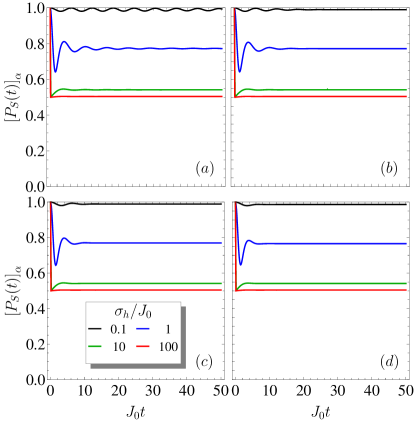
Figure 8: Plot of the disorder-averaged return probability, $\left[P_{S}(t)\right]_{\alpha}$, as a function of time for different values of $\sigma_{h}$, as indicated in the plot, with the initial state $\ket{\psi(0)}=\ket{S}$, for (a) $\sigma_{J}=0$, (b) $\sigma_{J}=0.1J_{0}$, (c) $\sigma_{J}=0.2J_{0}$, (d) $\sigma_{J}=0.3J_{0}$.

Figure 9: Plot of the steady-state disorder-averaged return probability, $\left[P_{S}(t)\right]_{\alpha}$ as a function of $\sigma_{h}$ for $\sigma_{J}=0$ with the initial state $\ket{\psi(0)}=\ket{S}$.

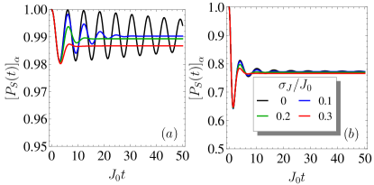
Figure 10: Plot of the disorder-averaged return probability, $\left[P_{S}(t)\right]_{\alpha}$, as a function of time for different values of $\sigma_{J}$, as indicated in the plot, with the initial state $\ket{\psi(0)}=\ket{S}$, for (a) $\sigma_{h}=0.1J_{0}$, (b) $\sigma_{h}=J_{0}$. Note the different scales on these two plots for the vertical axis compared both to the results for the “classical” state and to each other.

IV Ising coupling

We now proceed to study the temporal dynamics of two capacitively coupled singlet-triplet qubits, described by the disordered Ising Hamiltonian in Eq. (6).

We model the charge noise and the Overhauser noise using a random exchange coupling within each singlet-triplet qubit and a random on-site magnetic field, respectively. We focus on the experimentally relevant regime dominated by the Overhauser disorder, and we consider only static noise, a working assumption justified by the slow dynamics of the nuclear spins relative to the electron spins. The exchange couplings $J_{i}\geq 0$ ($i=1,2$) are drawn independently from a Gaussian distribution with mean $J_{0}$ and variance $\sigma_{J}^{2}$ truncated to non-negative values, whereas the magnetic fields $h_{i}$ ($i=1,2$) are drawn independently from a Gaussian distribution with mean $h_{0}$ and variance $\sigma_{h}^{2}$. The disordered model is thus specified by the dimensionless parameters $(\sigma_{J}/J_{0},\varepsilon J_{0},h_{0}/J_{0},\sigma_{h}/J_{0})$, with the first two controlling the inter-qubit coupling and the rest controlling single-qubit precession. We note that, unlike the Heisenberg case, the uniform applied magnetic field $h_{0}$ is now a relevant parameter in determining the qubit dynamics.

In the following we examine the time evolution of the return probability $\left|\braket{\psi(t)}{\psi(0)}\right|^{2}$ and the magnetization $\braket{\sigma_{i}^{x}}$ at each site $i$ for different initial states and different parameter settings.

IV.1 $\ket{\uparrow\downarrow}_{x}$ initial state

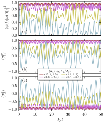
Figure 11: Dynamics of (a) the return probability and (b), (c) the single-site magnetizations starting from the initial state $\ket{\uparrow\downarrow}_{x}$, for a few typical disorder realizations of the Overhauser fields $(h_{1},h_{2})$. Here we use $\varepsilon=0.1J_{0}^{-1}$ and $J_{1}=J_{2}=J_{0}$, ignoring the charge noise $\sigma_{J}$.

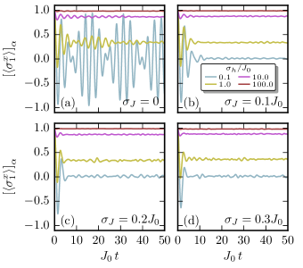
Figure 12: Disorder-averaged dynamics of the single-site magnetization starting from the initial state $\ket{\uparrow\downarrow}_{x}$, for various strengths of the charge noise $\sigma_{J}$ and the Overhauser noise $\sigma_{h}$.

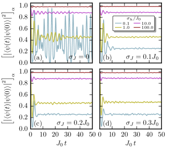
Figure 13: Disorder-averaged dynamics of the return probability starting from the initial state $\ket{\uparrow\downarrow}_{x}$, for various strengths of the charge noise $\sigma_{J}$ and the Overhauser noise $\sigma_{h}$.

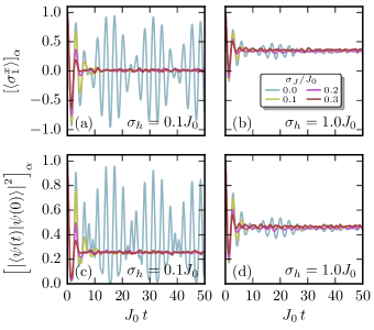
Figure 14: Effect of tuning $\sigma_{J}$ on the disorder-averaged dynamics of the single-site magnetization and the return probability, starting from the initial state $\ket{\uparrow\downarrow}_{x}$.

We first consider the time evolution starting from the product initial state $\ket{\uparrow\downarrow}_{x}$. Recall that we use $\ket{\uparrow}$ / $\ket{\downarrow}$ to denote the singlet/triplet state of a double quantum dot qubit. The $\ket{\uparrow\downarrow}_{x}$ state we consider here is polarized in the $x$ direction of the singlet/triplet basis, which represents the $\ket{\uparrow\downarrow\downarrow\uparrow}$ configuration of the individual quantum dots of the two-qubit system. We focus on the competition between the inter-qubit coupling and the Overhauser noise, ignoring the charge noise for now. Figure 11 shows the coupled qubit dynamics of the return probability and the single-site magnetizations for a few typical random realizations.

When the on-site magnetic field is weak, the two-qubit dynamics are driven mainly by the $J_{1}\sigma_{1}^{z}+J_{2}\sigma_{2}^{z}$ exchange terms and exhibit fast oscillations at a frequency around $J_{0}$ in the absence of charge noise. These fast oscillations are further modulated by the inter-qubit coupling term $\varepsilon J_{1}J_{2}\sigma_{1}^{z}\sigma_{2}^{z}$, and acquire a periodic envelope with a low frequency close to $\varepsilon$. Comparing the curves in each panel of Fig. 11, we find that increasing the local magnetic field $h_{i}$ accelerates the oscillation frequency and reduces the oscillation amplitude significantly. Eventually, the Overhauser terms overwhelm the exchange coupling, and the coupled qubits oscillate at a high frequency around $h_{i}$. At strong enough $h_{i}$, the magnetization at each site is essentially frozen to the initial value, and the return probability stays close to unity. This comes from the fact that the $\ket{\uparrow\downarrow}_{x}$ initial state becomes an approximate eigenstate of the two-qubit Hamiltonian in this limit.

The temporal dynamics of the coupled qubits are characterized by persistent oscillations with a frequency dependent upon the Overhauser fields and the exchange couplings. These fast oscillations are quickly wiped out upon averaging over the Overhauser disorder. Figures 12(a) and 13(a) show the disorder averaged dynamics of the single-site magnetization and the return probability for various strengths of the Overhauser noise $\sigma_{h}$, in the absence of the charge noise $\sigma_{J}$. For each parameter set we average over $10^{3}$ disorder realizations. This average over the Overhauser noise introduces three changes. First, the fast oscillations in both the return probability and the single-site magnetizations acquire a decaying envelope. The gradual decay of the oscillation amplitude is clearly visible even for very weak disorder at $\sigma_{h}=0.1J_{0}$. Second, the residual oscillations have a low frequency around $J_{0}$ controlled by the exchange coupling, largely independent from the Overhauser noise $\sigma_{h}$. This can be understood as an overall destructive interference from the disorder average over the random magnetic field $h_{i}$. Third, and most importantly, at strong Overhauser disorder $\sigma_{h}$, the local information in the initial $\ket{\uparrow\downarrow}_{x}$ state persists through the time evolution, as indicated by both the return probability and the single-site magnetizations.

Now that we have understood the role of the Overhauser noise $\sigma_{h}$, we move on to study the charge noise $\sigma_{J}$. Figures 12 and 13 show the effect of adding a moderate $\sigma_{J}$ on the disorder-averaged temporal dynamics of the return probability and the single-site magnetizations. We find that a nonzero $\sigma_{J}$ further suppresses the oscillatory dynamics and accelerates the approach to the final steady state, which is also clearly visible in Fig. 14. This suppression comes from the mainly destructive interference between the random values of the exchange couplings $J_{i}$, and it erases the oscillations of frequency $\sim J_{0}$ except for the first few periods. This effect of $\sigma_{J}$ on the transient dynamics is more pronounced when $\sigma_{h}$ is weak. Crucially, we find that a weak charge noise $\sigma_{J}$ does not modify the final steady-state values of the return probability or the single-site magnetizations, even when $\sigma_{J}$ is stronger than the Overhauser noise $\sigma_{h}$.

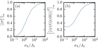
Figure 15: The Overhauser noise dependence of (a) the steady-state magnetization and (b) the steady-state return probability for the initial state $\ket{\uparrow\downarrow}_{x}$.

Therefore, we turn back to the Overhauser noise $\sigma_{h}$ and take a closer look at its effect on the asymptotic retention of memory of the initial state in the final steady state. Figure 15 shows the steady-state magnetization and the steady-state return probability, as functions of the Overhauser noise $\sigma_{h}$. In both cases, we find a steady enhancement of the initial-state memory retention as $\sigma_{h}$ increases. Despite the absence of a sharp transition (as is typical in such small systems), we note that a moderate $\sigma_{h}$ (around a few $J_{0}$) is enough to incur a significant boost to the preservation of the initial collective state.

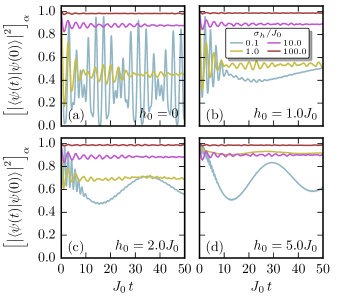
Figure 16: Disorder-averaged dynamics of the return probability to the initial state $\ket{\uparrow\downarrow}_{x}$ for various strengths of the mean magnetic field $h_{0}$ and the Overhauser noise $\sigma_{h}$, in the absence of the charge noise $\sigma_{J}$.

Finally, we discuss the effect of adding a nonzero mean value $h_{0}$ to the random magnetic field distribution. Experimentally, this amounts to applying an external, uniform magnetic field to the two-qubit system. Figure 16 shows the response of the disorder-averaged return probability dynamics to the mean magnetic field $h_{0}$. We find that when the Overhauser noise $\sigma_{h}$ is relatively weak, applying a uniform magnetic field $h_{0}$ enhances the preservation of the initial $\ket{\uparrow\downarrow}_{x}$ state. In this regime, the uniform magnetic field also suppresses the residual oscillations in the disorder-averaged dynamics of the return probability.

IV.2 Singlet initial state

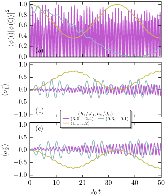
Figure 17: Dynamics of (a) the return probability and (b,c) the single-site magnetizations starting from the singlet initial state $\ket{S}$ for a few typical disorder realizations of the Overhauser fields $(h_{1},h_{2})$. Here we use $\varepsilon=0.1J_{0}^{-1}$ and $J_{1}=J_{2}=J_{0}$, ignoring the charge noise $\sigma_{J}$.

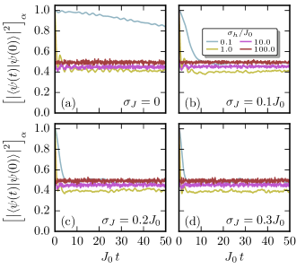
Figure 18: Disorder-averaged dynamics of the return probability starting from the singlet initial state $\ket{S}$, for various strengths of the charge noise $\sigma_{J}$ and the Overhauser noise $\sigma_{h}$.

As a second example, we examine the time evolution starting from the singlet state $\ket{S}=\frac{1}{\sqrt{2}}(\ket{\uparrow\downarrow}-\ket{\downarrow\uparrow})$. We emphasize that $\ket{S}$ is the singlet state of the pair of logical qubits, conceptually different from the singlet state $\ket{\uparrow}$ of each individual double quantum dot qubit. In contrast to the $\ket{\uparrow\downarrow}_{x}$ state considered earlier, $\ket{S}$ is not a product state or an approximate eigenstate of the strongly disordered Hamiltonian. Accordingly, the time evolution starting from $\ket{S}$ has a qualitatively different response to environmental noise.

Figure 17 shows the dynamics of the return probability and the single-site magnetizations for a few typical Overhauser disorder realizations in the absence of the charge noise. Notice that the initial singlet state $\ket{S}$ is an eigenstate of the Hamiltonian in the clean limit with a uniform exchange coupling $J_{1}=J_{2}(=J_{0})$ and a uniform magnetic field $h_{1}=h_{2}$, with eigenvalue $-\varepsilon J_{0}^{2}$. As the magnetic field imbalance $h_{1}-h_{2}$ increases, the return probability develops persistent oscillations with a large amplitude and no asymptotic steady state, indicating the erasure of the local information in the initial state. Similar persistent oscillations are also visible in the magnetization dynamics.

This indicates that the time evolution following the singlet initial state $\ket{S}$ is very susceptible to disorder, in sharp contrast to the $\ket{\uparrow\downarrow}_{x}$ initial state. To see this point more clearly, we perform an average over $10^{3}$ disorder realizations for each parameter set. Figure 18 shows the disorder averaged dynamics of the return probability for various strengths of the Overhauser noise $\sigma_{h}$ and the charge noise $\sigma_{J}$. (Here we focus on the return probability because the magnetization vanishes after disorder averaging.) We find that, for any appreciable amount of disorder, the averaged return probability drops to around $0.5$ within a time span as short as a few $J_{0}^{-1}$, and this descent accelerates as either type of disorder increases. To understand the asymptotic behavior at long time, recall from Fig. 17(a) that the single-realization dynamics of the return probability exhibits persistent oscillations with peak-to-peak amplitude close to unity. The final value of the averaged return probability around $0.5$ under strong disorder thus reflects the lack of an asymptotic steady state of the time evolution starting from the singlet initial state for each disorder realization.

To sum up, the singlet initial state shows no sign of memory retention at strong disorder, and the erasure of the initial state memory is accelerated by an increase in either the Overhauser noise or the charge noise.

V Conclusion

We have calculated the two-qubit dynamical evolution in the “always on” configuration of two coupled spin qubits in semiconductors where the coupling could be either just an exchange coupling (i.e., Heisenberg-type) or a dipolar capacitive coupling (i.e., Ising-type). The central theme of the work is studying spin qubit dynamics in the presence of both qubit interactions and qubit noise (with the noise being a random magnetic field at each qubit and/or the interqubit coupling itself being noisy due to environmental fluctuations corresponding qualitatively to Overhauser noise and charge noise respectively). Our work is directly relevant for experiments on exchange-coupled spin qubits and capacitively coupled singlet-triplet qubits when the inter-qubit coupling is kept on throughout the experiment.

Our main finding is that the disorder-averaged quantum qubit dynamics are oscillatory in time with the oscillation decay controlled by the noise strength. The most striking feature of the qubit dynamics in the presence of noise that we find is a noise-induced quantum memory effect that can be directly studied experimentally using currently existing laboratory spin qubits. All that one needs to be able to do is prepare either the “classical” $\ket{\uparrow\downarrow}$ state or the singlet state, $\ket{S}$, and be able to control the exchange coupling. While it is true that the magnetic disorder strength, $\sigma_{h}$, cannot be controlled in an actual experiment, one does have control over the dimensionless quantity, $\sigma_{h}/J_{0}$, via the exchange coupling, and this is what we adjust in our theoretical calculations. In experiments, one finds that $\sigma_{J}$ is roughly proportional to $J_{0}$, so that $\sigma_{J}/J_{0}$ is a constantBarnesPrivComm . This would enable one to perform the necessary experiments to test our predictions, which simply requires obtaining the return probability as a function of time, as well as the steady-state return probability.

In particular, we find that in many situations the steady-state probability of the final state at long times being the initial state is very high, and that this “memory retention” effect, in fact, is enhanced by noise—the more noisy the system, the more likely it is that the final two-qubit state (after the oscillations have been damped out by noise) would essentially be exactly the same as the initial state in spite of time evolution under an arbitrary interqubit interaction! We provide detailed numerical and theoretical results for the steady-state return probability (i.e., the probability that the final state of the system is the same as the initial state after the qubits have evolved dynamically for a long time under the interqubit coupling) and the steady-state local magnetization to establish the noise-induced memory preservation of the two-qubit system. We emphasize that our finding of the “memory retention” effect in the coupled two-qubit dynamics is quite nontrivial and counterintuitive as it happens even when the magnetic field noise is not particularly strong, e.g., only of the order of the interqubit coupling. We have demonstrated in a previous workBarnesPRB2016 that “memory retention” effects occur in Heisenberg-coupled chains of four and six spins; in fact, these effects are even more pronounced in the four- and six-spin systems. These effects may be viewed as a “remnant” of many-body localization, which, strictly speaking, only happens in an infinitely long chain. We have therefore demonstrated in the current work that some qualitative manifestation of many-body localization already happens in a two-spin system, making an experimental demonstration of such effects feasible in existing semiconductor spin qubit platformsR2 ; R3 ; R4 ; R5 ; R6 ; R7 ; R8 .

We emphasize that the qubit dynamics depend on the initial state, and there are initial states for which memory retention fails, but our concrete dynamical results for various initial states should help guide experimental work studying qubit dynamics for spin qubits with exchange (“Heisenberg”) and capacitive (“Ising”) coupling. We also mention that our quasi-static approximation for noise is quantitatively accurate for the Overhauser noise (and is only qualitatively valid for the charge noise affecting the interqubit coupling). Therefore, our detailed numerical results and the associated qualitative conclusions are valid mainly for situations where the charge noise is not very large (or at least, not much larger than the Overhauser noise). This makes our conclusions apply more to GaAs-based spin qubit systems than Si systems since the Overhauser noise is typically not the limiting factor in Si-based spin qubits. Generalizing our work to situations involving general time-dependent noise is left for the future since such theories would necessitate accurate quantitative information regarding the noise dynamical spectral function not currently available in the literature.

Appendix A Analytical results for the Ising model

In this Appendix we provide an analytical formula, previously obtained in Ref. WangNPJQE, , for the time evolution governed by the Ising Hamiltonian for two capacitively coupled singlet-triplet qubits [Eq. (6)],

$$H=K\,\sigma_{1}^{z}\sigma_{2}^{z}+J_{1}\sigma_{1}^{z}+J_{2}\sigma_{2}^{z}+h_{1}\sigma_{1}^{x}+h_{2}\sigma_{2}^{x},$$

with $K=\varepsilon J_{1}J_{2}$.

The energy eigenvalues $E_{l}$ ($l=1,2,3,4$) of the $4\times 4$ matrix $H$ are given by the roots of the characteristic polynomial

$$p(E)=E^{4}-2aE^{2}-8bE+(K^{4}+2cK^{2}+d^{2}),$$ (23)

with coefficients

$$a =h_{1}^{2}+h_{2}^{2}+J_{1}^{2}+J_{2}^{2}+K^{2},$$ (24)

$$b =J_{1}J_{2}K,$$

$$c =h_{1}^{2}+h_{2}^{2}-J_{1}^{2}-J_{2}^{2},$$

$$d =h_{1}^{2}-h_{2}^{2}+J_{1}^{2}-J_{2}^{2}.$$

In terms of the quartic roots $E_{l}$, we can express the time evolution operator $U(t)=e^{-iHt}$ as

$$U(t)=\sum_{l=1}^{4}\frac{e^{-iE_{l}t}}{4M_{l}}\big{(}M_{l}+u^{x}_{1l}\sigma_{1}^{x}+u^{x}_{2l}\sigma_{2}^{x}+u^{z}_{1l}\sigma_{1}^{z}+u^{z}_{2l}\sigma_{2}^{z}\\ +u^{xz}_{l}\sigma_{1}^{x}\sigma_{2}^{z}+u^{zx}_{l}\sigma_{1}^{z}\sigma_{2}^{x}+u^{xx}_{l}\sigma_{1}^{x}\sigma_{2}^{x}+u^{yy}_{l}\sigma_{1}^{y}\sigma_{2}^{y}+u^{zz}_{l}\sigma_{1}^{z}\sigma_{2}^{z}\big{)},$$

with coefficients

$$M_{l} =E_{l}^{3}-aE_{l}-2b,$$ (25)

$$u^{x}_{1l} =h_{1}(E_{l}^{2}-d-K^{2}),\;u^{x}_{2l}=h_{2}(E_{l}^{2}+d-K^{2}),$$

$$u^{z}_{1l} =J_{1}E_{l}^{2}+2J_{2}KE_{l}+J_{1}(K^{2}-d),$$

$$u^{z}_{2l} =J_{2}E_{l}^{2}+2J_{1}KE_{l}+J_{2}(K^{2}+d),$$

$$u^{xz}_{l} =2h_{1}(J_{2}E_{l}+J_{1}K),\;u^{zx}_{l}=2h_{2}(J_{1}E_{l}+J_{2}K),$$

$$u^{xx}_{l} =2h_{1}h_{2}E_{l},\;u^{yy}_{l}=-2h_{1}h_{2}K,$$

$$u^{zz}_{l} =KE_{l}^{2}+2J_{1}J_{2}E_{l}-K(K^{2}+c).$$

References

- (1) F. Zwanenburg, A. S. Dzurak, A. Morello, M. Y. Simmons, L. C. L. Hollenberg, G. Klimeck, S. Rogge, S. N. Coppersmith, and M. A. Eriksson, Rev. Mod. Phys. 85, 961 (2013).
- (2) J. Pla, K. Y. Tan, J. P. Dehollain, W. H. Lim, J. J. L. Morton, D. N. Jamieson, A. S. Dzurak, and A. Morello, Nature 489, 541 (2012).
- (3) J. Pla, K. Y. Tan, J. P. Dehollain, W. H. Lim, J. J. L. Morton, F. A. Zwanenburg, D. N. Jamieson, A. S. Dzurak and A. Morello, Nature 496, 334 (2013).
- (4) M. Veldhorst, J. C. C. Hwang, C. H. Yang, A. W. Leenstra, B. de Ronde, J. P. Dehollain, J. T. Muhonen, F. E. Hudson, K. M. Itoh, A. Morello, and A. S. Dzurak, Nat. Nano. 9, 981 (2014).
- (5) B. Maune, M. G. Borselli, B. Huang, T. D. Ladd, P. W. Deelman, K. S. Holabird, A. A. Kiselev, I. Alvarado-Rodriguez, R. S. Ross, A. E. Schmitz, M. Sokolich, C. A. Watson, M. F. Gyure, and A. T. Hunter, Nature 481, 344 (2012).
- (6) D. Kim, Zhan Shi, C. B. Simmons, D. R. Ward, J. R. Prance, T. S. Koh, J. K. Gamble, D. E. Savage, M. G. Lagally, M. Friesen, S. N. Coppersmith, and M. A. Eriksson, Nature 511, 70 (2014).
- (7) M. Shulman, S. P. Harvey, J. M. Nichol, S. D. Bartlett, A. C. Doherty, V. Umansky, and A. Yacoby, Nat. Commun. 5, 5156 (2014).
- (8) O. E. Dial, M. D. Shulman, S. P. Harvey, H. Bluhm, V. Umansky, and A. Yacoby, Phys. Rev. Lett. 110, 146804 (2013).
- (9) S. Foletti, H. Bluhm, D. Mahal, V. Umansky, and A. Yacoby, Nat. Phys. 5, 903 (2009).
- (10) F. Martins, F. K. Malinowski, P. D. Nissen, E. Barnes, S. Fallahi, G. C. Gardner, M. J. Manfra, C. M. Marcus, and F. Kuemmeth, Phys. Rev. Lett. 116, 116801 (2016).
- (11) J. Medford, J. Beil, J. M. Taylor, E. I. Rashba, H. Lu, A. C. Gossard, and C. M. Marcus, Phys. Rev. Lett. 111, 050501 (2013).
- (12) M. Veldhorst, C. H. Yang, J. C. C. Hwang, W. Huang, J. P. Dehollain, J. T. Muhonen, S. Simmons, A. Laucht, F. E. Hudson, K. M. Itoh, A. Morello, and A. S. Dzurak, Nature 526, 410 (2016).
- (13) K. Nowack, M. Shafiei, M. Laforest, G. E. D. K. Prawiroatmodjo, L. R. Schreiber, C. Reichl, W. Wegscheider, and L. M. K. Vandersypen, Science 333, 1269 (2011).
- (14) M. Shulman, O. E. Dial, S. P. Harvey, H. Bluhm, V. Umansky, and A. Yacoby, Science 336, 202 (2012).
- (15) M. Simmons, unpublished and private communication; A. Yacoby, private communication.
- (16) X. Hu and S. Das Sarma, Phys. Rev. Lett. 96, 100501 (2006).
- (17) W. M. Witzel and S. Das Sarma, Phys. Rev. Lett. 98, 077601 (2007).
- (18) Ł. Cywiński, W. M. Witzel, and S. Das Sarma, Phys. Rev. Lett. 102, 057601 (2009).
- (19) E. Barnes, Ł. Cywiński, and S. Das Sarma, Phys. Rev. Lett. 109, 140403 (2012).
- (20) Ł. Cywiński, R. M. Lutchyn, C. P. Nave, and S. Das Sarma, Phys. Rev. B77, 174509 (2008).
- (21) D. Loss and D. P. DiVincenzo, Phys. Rev. A57, 120 (1998).
- (22) D. P. DiVincenzo, D. Bacon, J. Kempe, G. Burkard, and K. B. Whaley, Nature 408, 339 (2000).
- (23) X. Hu and S. Das Sarma, Phys. Rev. A61, 062301 (2000).
- (24) V. W. Scarola and S. Das Sarma, Phys. Rev. A71, 032340 (2005).
- (25) F. A. Calderon-Vargas and J. P. Kestner, Phys. Rev. B91 035301 (2015).
- (26) V. Srinivasa and J. M. Taylor, Phys. Rev. B92, 235301 (2015).
- (27) J. Levy, Phys. Rev. Lett. 89, 147902 (2002).
- (28) J. R. Petta, A. C. Johnson, J. M. Taylor, E. A. Laird, A. Yacoby, M. D. Lukin, C. M. Marcus, M. P. Hanson, A. C. Gossard, Science 309, 2180 (2005).
- (29) W. A. Coish and D. Loss, Phys. Rev. B72, 125337 (2005).
- (30) D. Klauser, W. A. Coish, and D. Loss, Phys. Rev. B73, 205302 (2006).
- (31) E. Barnes, D.-L. Deng, R. E. Throckmorton, Y.-L. Wu, and S. Das Sarma, Phys. Rev. B93, 085420 (2016).
- (32) X. Wang, E. Barnes, and S. Das Sarma, npj Quantum Information 1, 15003 (2015).
- (33) E. Barnes, private communication.