gevolution: a cosmological N-body code based on General Relativity
Abstract
We present a new N-body code, gevolution, for the evolution of large scale structure in the Universe. Our code is based on a weak field expansion of General Relativity and calculates all six metric degrees of freedom in Poisson gauge. N-body particles are evolved by solving the geodesic equation which we write in terms of a canonical momentum such that it remains valid also for relativistic particles. We validate the code by considering the Schwarzschild solution and, in the Newtonian limit, by comparing with the Newtonian N-body codes Gadget-2 and RAMSES. We then proceed with a simulation of large scale structure in a Universe with massive neutrinos where we study the gravitational slip induced by the neutrino shear stress. The code can be extended to include different kinds of dark energy or modified gravity models and going beyond the usually adopted quasi-static approximation. Our code is publicly available.
This is an author-created, un-copyedited version of an article published in JCAP. IOP Publishing Ltd is not responsible for any errors or omissions in this version of the manuscript or any version derived from it. The Version of Record is available online at http://dx.doi.org/10.1088/1475-7516/2016/07/053.
1 Introduction
Almost to the day 100 years ago, Einstein presented his theory of General Relativity (GR) to the Royal Prussian Academy of Sciences [1]. This completely transformed our view on gravitation. Spacetime is no longer understood as an absolute element, a fixed stage on which interactions take place, but as a dynamical entity which takes part in the interactions. Nowhere is this more apparent than in cosmology, where the dynamics imply that our Universe can not be in an eternal “steady-state”. From Lemaître’s and Hubble’s discovery of the expansion law [2, 3] to the latest precision measurements of cosmic microwave background anisotropies [4] we have collected ample evidence that our Universe has expanded and evolved from a very hot and fairly uniform initial state (the hot big bang which probably was preceded by an inflationary phase) into the present cold and highly differentiated state. The fact that all current observations can be consistently interpreted in the context of GR, giving rise to the CDM concordance model of cosmology, is arguably one of the greatest successes of Einstein’s theory of gravity.
This concordance model achieves a good fit to the data only by two phenomenological postulates, the existence of two “dark” contributors of stress-energy. Non-baryonic Dark Matter (DM) outweighs ordinary matter (atoms and ionized gas) by more than 5:1 and is therefore the dominant driver for gravitational clustering. It is usually modelled as a yet-to-be-found weakly interacting massive particle. Dark Energy (DE) is an even more exotic entity which effectively acts like a cosmological constant and gives rise to accelerated expansion. One should keep in mind that evidence for these dark components remains circumstantial at this point, as we only observe their apparent gravitational effects. Major efforts are being undertaken to obtain a deeper understanding of DM and DE at the fundamental level. In particular the study of cosmic large scale structure with high precision seems to be a promising avenue, and many upcoming surveys [5, 6, 7] are targeting more precise measurement of DM and DE properties via their gravitational interaction. Other experiments, so called direct and indirect DM searches, aim to detect DM also via non-gravitational interactions [8].
The theoretical modelling of the formation of large scale structure is very challenging at nonlinear scales. Computer simulations have a long tradition in this field, and due to technological advancement, continue to keep pace with the increasing data quality of astronomical observations. However, these simulations generally still use Newton’s law of gravitation. This has spurred an extensive debate in the literature whether and how this approximation can be justified in the current era of precision cosmology [9, 10, 11, 12, 13]. It seems that the Newtonian approach works fairly well within the context of the CDM model. Firstly, if one neglects radiation in the late Universe, the only source of perturbations is nonrelativistic matter. A Newtonian scheme would clearly be unsuitable for relativistic sources. Furthermore, there is a separation of scales between the nonlinear scale and the cosmological horizon. A Newtonian scheme is ignorant about the presence of a horizon, but it turns out that linear perturbations of nonrelativistic matter can be identified with quantities of linear perturbation theory of GR. One can therefore find a consistent interpretation of Newtonian simulations also at very large scales [13], but only at the linear level and one has to be very careful about gauge issues. The presence of radiation also has a small effect on the evolution of structure which is difficult to account for within a Newtonian framework.
Despite these subtleties, models beyond CDM have been studied with simulation codes using some modified Newtonian approaches [14, 15, 16, 17]. These codes are customized towards specific models where appropriate approximations (such as the quasi-static limit which is only valid on small scales and for small enough speed of sound, see [18] for a discussion) can be justified. However, a general framework would be desirable in order to access the entire space of viable models. We have therefore developed a new N-body code which is completely based on GR [19]. The aim of this paper is to introduce the code and explain in detail its theoretical underpinning. As we make our code available to the community, this paper also serves as a first introduction for future users. From the very beginning we avoid any reference to the Newtonian picture and follow a conceptually clean approach which ensures self-consistency and compliance with GR principles at every step. The central element of our framework is a weak field expansion, meaning that we are able to treat any settings where no strong gravitational fields appear. This, of course, includes any setting where the Newtonian approximation would be applicable, but also arbitrary scenarios with relativistic sources as long as gravitational fields are not very strong. The framework is well suited for cosmology, but it could also be fruitful for astrophysical applications with moderate gravitational fields where a Newtonian treatment is insufficient.
Let us also clarify the relation between our framework and other numerical approaches such as the ones of [20, 21]. While those approaches do not rely on a weak field expansion, allowing access to the strong field regime, they are based on a fluid description of the matter sources. The fluid approximation is valid for DM only as long as nonlinear collapse has not yet caused the trajectories of mass elements to cross each other, at which point the fluid equations become singular. This phenomenon, sometimes called shell-crossing, is ubiquitous during the process of nonlinear clustering of effectively collisionless matter. It is an essential aspect of hierarchical structure formation and the virialization of DM halos. In practice this means that approaches based on the fluid description are expected to break down at the nonlinear scale while a weak field N-body scheme should be able to cover all the scales down to the occurrence of strong fields. In the present Universe the nonlinear scale is at some tens of megaparsecs while the largest strong field regions222Our notion of strong fields is actually gauge dependent. We are working in Poisson gauge where metric perturbations become large as one approaches the Schwarzschild radius. However, the tidal forces are very small at the Schwarzschild horizon of a supermassive black hole, and one could find a gauge where this region would be classified as weak field regime. are supermassive black holes with a radius of a few hundred astronomical units, i.e. in the range of milliparsecs. Therefore, while certainly interesting for the study of some idealized setups, the fluid approaches are of limited use for the modelling of realistic cosmological structures.
In Section 2 we derive the equations which govern the evolution of the metric and hence of spacetime geometry. These are formulated in a way which is convenient for numerical integration but also intuitive for any cosmologist familiar with relativistic perturbation theory. Section 3 discusses the ensemble of N-body particles, in particular its stress-energy and its evolution under gravity. The numerical implementation is outlined in Section 4. Some first simulation results are presented in Section 5, ranging from verification checks to cosmological applications. We carry out some simulations with relativistic particle species, a setting for which Newtonian codes are severely limited. Our results are summarized in Section 6. Some technical aspects of our code are explained in three appendices. More detailed instructions for users of the code can be found in the public release at https://github.com/gevolution-code/gevolution-1.0.git.
2 Einstein’s equations
We start by writing an ansatz for the line element, which for our purposes shall take the form of a perturbed Friedman-Lemaître-Robertson-Walker (FLRW) metric in Poisson gauge,
| (2.1) |
where is a background scale factor (the choice of background is discussed below), is conformal time, and are comoving Cartesian coordinates. As usual we follow the convention that summation is implied for repeated indices, where letters from the Latin alphabet specify space-like indices and letters from the Greek alphabet run over all four spacetime dimensions. We also use the shorthands and to denote partial derivatives, to denote the spatial Laplace operator, and to denote index symmetrization.
The Poisson gauge is usually introduced at linear level, but we maintain the gauge conditions even though we go beyond perturbation theory. Our gauge conditions can be maintained as long as we remain in our weak-field setting where all gravitational fields (, , and ) are small. In fact, our expansion remains linear in and (though not in , ) such that they can be directly interpreted as the usual spin-1 and spin-2 perturbations familiar from perturbation theory. In other words, is the spin-1 field responsible for frame dragging, whereas carries the two spin-2 degrees of freedom of gravitational waves or more general tensor perturbations.
The metric of eq. (2.1) is of course motivated having a cosmological application in mind. However, if one wants to use our framework to describe perturbations around a Minkowski geometry instead of FLRW, as would be appropriate for astrophysical applications, one can simply set and in all our equations. An example is discussed in Section 5.1.
The metric variables, i.e. for the background and , , , for the perturbations, are evolved according to Einstein’s field equations,
| (2.2) |
where is the Einstein tensor (a quantity built from the metric and its first and second derivatives) and is the stress-energy tensor. For a generic model we write the total action as
| (2.3) |
where is the metric determinant, is the Ricci scalar and is the matter Lagrangian which usually depends on and matter variables. We use the convention that a possible cosmological constant would be included in the matter Lagrangian. The action principle requires that the variation with respect to vanishes, which implies
| (2.4) |
Working out the left hand side, we obtain , where is the Ricci tensor. This means that the stress-energy tensor is related to the matter Lagrangian by
| (2.5) |
In the following subsections we explain how eq. (2.2) can be written in a convenient form by using our ansatz for the metric, eq. (2.1), and employing a judicious expansion in the metric perturbation variables.
2.1 Choice of background
In linear perturbation theory the background is usually defined as the model which is obtained in the limit where perturbations are taken to zero. This is not necessarily a good prescription beyond the linear level, since there are nonlinear terms which do not average to zero on the space-like hypersurface and therefore could give a relevant correction to the “average” evolution of the geometry. This is one aspect of the well known “backreaction” problem (see [22, 23] for recent reviews and [24] for a discussion in the present framework). Instead of trying to address this problem by giving a prescription of how to construct the background in general, we follow a different philosophy. We note that there is a residual gauge freedom which allows for some degree of arbitrariness in the background model: a small change to the background can be absorbed into the perturbation variables to leave the line element (2.1) invariant. Evidently, and may acquire a homogeneous mode by this gauge transformation, but we allow for this as long as this homogeneous mode remains a small perturbation and does not spoil the weak field expansion which is elaborated in the next subsection.
Effectively we conjecture that, even though perturbations of the stress-energy can become arbitrarily large, there may still exist a coordinate system and a choice of background model such that the geometry can be described by eq. (2.1) where all metric perturbation variables are small. Since we start our simulations at a time where perturbation theory is still valid, we know that this conjecture holds initially333There are cases where linear perturbation theory is valid (and the geometry therefore remains close to FLRW) but and become large. But this can happen only on super-Hubble scales as must remain small for perturbation theory to be valid. Here denotes a typical component of the Weyl curvature while is a typical component of the background Ricci tensor. This, however, means that it is a gauge other than the Poisson gauge in which the perturbation variables remain small. An example of this behavior is dilaton inflation [25]. Such scenarios are not the topic of this work.. We can monitor the perturbations during the evolution to make sure that the weak field expansion remains valid at all times. If, for instance, our background model turns out to be inadequate, the system reacts by generating large homogeneous modes in and (see Section 5.3 for an explicit demonstration) which eventually would break the scheme. In this case the background model has to be improved. We do not provide a general set of conditions under which an appropriate background can be found, but we can address the backreaction problem on a case-by-case basis by solving the equations and monitoring the size of the geometric perturbation variables. On the other hand, the smallness of and (and of the other metric perturbations) is a sufficient condition to ensure that the geometry is close to the chosen background and that the weak field expansion discussed in the next section is valid.
Let us now turn to the aforementioned residual gauge freedom. We can actually exploit this gauge freedom to make a convenient choice for the background model. We only have to make sure that the homogeneous modes in the perturbations remain small enough such that we still trust our evolution equations. The background model (and associated parameters such as ) therefore is in this sense gauge dependent, but of course observables are not. Once an experimental setup is specified, the outcome is independent of the choice of gauge. This choice just specified which part is considered as belonging to the background and which part as belonging to the perturbations. We make a convenient choice for the background stress-energy tensor , which determines the scale factor according to Friedmann’s equation,
| (2.6) |
The perturbations are then solved by using Einstein’s equations with the background contributions subtracted, for instance
| (2.7) |
which does not introduce any assumptions about the background model. We only require that the metric perturbations , , and remain small on this background. The homogeneous modes of the perturbation variables are computed consistently such that the observables do not depend on the precise choice of . A numerical study of this issue is presented in Section 5.3.
We finally note that we still have not exhausted the gauge freedom completely. We can rescale our spatial coordinates such that the homogeneous mode of takes a particular value at a given instance in time. This can be done only once, the homogeneous mode at all other times being determined by the dynamics. We use this freedom to set the homogeneous mode of to zero at the initial time of the simulation. We can also rescale the time coordinate to redefine the homogeneous mode of . As opposed to the previous case the dynamics do not determine the evolution of this mode. Instead, we can fix any functional form of this mode, and the dynamics of all other variables is then automatically solved with respect to the corresponding choice of time coordinate. For convenience, in our code the homogeneous mode of is set equal to the one of , so that the homogeneous mode of vanishes. Again, these choices do not have any effect at the level of observables.
2.2 Weak field expansion
In order to reduce the ten nonlinear coupled partial differential equations of eq. (2.2) to a tractable set of evolution equations for the perturbation variables, we employ a weak field expansion. The assumption behind this scheme is that there are no strong gravitational fields at the scales of interest. It should be stressed that this does not imply that the perturbations of the stress-energy tensor, which are the sources of the gravitational fields, have to remain small. In fact, is generally much larger than inside dense regions. As an example, our solar system perfectly fits into a weak field description, despite the fact that the density varies by some 25 orders of magnitude between the center of the sun ( g/cm3) and the average matter density in the interplanetary medium ( g/cm3 at AU from the sun). A weak field expansion amounts to an expansion in terms of the metric perturbations alone, without at the same time employing any expansion of the matter variables. It is not equivalent to a post-Newtonian expansion, which is an expansion in inverse powers of the speed of light. Such an expansion would be suitable only as long as the perturbations of stress-energy are non-relativistic to a good approximation. We do not place this restriction on our stress-energy tensor (the relation between our scheme and a post-Newtonian one [26] is discussed in more detail in [27]).
Empirically we know that the scalar perturbations , are generally much larger than the spin-1 and spin-2 perturbations and . This is why Newtonian simulations could enjoy such a successful history. While the gravitational potential can be easily observed with a table-top experiment [28], there are only few experiments which were able to detect frame dragging directly (e.g. [29, 30]), and a direct observation of gravitational waves has only recently been achieved [31] as the result of a remarkable technological feat. When expanding Einstein’s equations (2.2) in terms of the metric perturbations, we therefore keep only the linear terms444In our previous works [27, 32] we claimed that we keep all quadratic terms with two spatial derivatives, which would have included terms built with or . In fact, we then dropped these terms from the equations without mention. A technical justification for this step is given in [10], but it relies on some restrictive assumptions about the stress-energy tensor which we would like to relax. We admit that a general model could have relativistic sources creating large spin-1 and spin-2 metric perturbations, but when quadratic terms in these variables become relevant, we do not consider this a weak field setting anymore and therefore our framework would be inappropriate. for and . However, for the scalar potentials and we are more cautious. We assume that the potentials are small everywhere, but we admit that they have fluctuations at small scales which can lead to large density fluctuations: can become much larger than unity. This reflects the Newtonian gravitational instability, which is also the only instability of General Relativity. Curvature, which is related to the spatial Laplacian of and therefore becomes large at small scales. In order to appreciate this effect, we keep the quadratic terms of and with the highest number of spatial derivatives. Since the differential equations are second order, the highest possible number is two.
However, as we will see below, the difference of the two potentials,
| (2.8) |
is determined from the same set of equations as and . We therefore treat on the same footing as the spin-1 and spin-2 perturbations. In other words, while we keep some quadratic terms in , after systematically replacing by , we will only keep terms linear in .
To summarize, we keep all terms up to linear order in the metric perturbations without distinction, but from the quadratic ones we only keep the ones built with which have exactly two spatial derivatives. Examples are or . Terms like , or all other higher-order terms are subleading and are dropped. We argue that this truncation contains all the relevant terms to compute , and correctly at leading order555In cases where relativistic sources on the right hand side of eq. (2.10) dominate over the second-order terms of the weak field expansion, the metric perturbations are still determined correctly at leading order – in this case the second-order contributions should be considered subleading. An explicit example will be given in Section 5.4., even in situations where they are strongly suppressed666Note, for instance, that our expansion agrees with a calculation in second-order perturbation theory of CDM in the regime where the latter is valid. If we ignore primordial vector and tensor contributions, the only first-order perturbations are scalars. At second order, , and are sourced by terms quadratic in the first-order perturbations. We use the space-space components of Einstein’s equations to determine , and . To acquire the correct number of spacetime indices, any term built from the linear scalar perturbations needs to have two spatial derivatives in order to appear in this equation. Our expansion therefore keeps all the relevant terms for a second-order calculation. Our stress-energy tensor, however, is computed nonperturbatively. It coincides with the second-order one whenever second-order perturbation theory is valid, but it remains valid also beyond this regime. (such as CDM standard cosmology). In fact, this can be understood as the guiding principle of our weak field expansion: we construct a scheme which provides a meaningful calculation of all the relativistic terms that perturb the geometry and are missed by a Newtonian treatment.
Applying the expansion to the time-time component of Einstein’s equation, eq. (2.7), we obtain
| (2.9) |
If one wants to draw the analogy to a Newtonian scheme, this is the equation which replaces the Poisson equation . We use this equation to determine the evolution of . The remaining perturbation variables are determined from the traceless part of the space-space set of Einstein’s equations which have no Newtonian analog. In terms of the weak field expansion they read
| (2.10) |
where we introduced the anisotropic stress tensor . Due to the subtraction of the trace, these are five independent equations, exactly the number needed in order to determine (scalar), (two polarizations) and (two polarizations).
The remaining four Einstein’s equations, namely the time-space equations and the spatial trace are redundant, they follow from the above equations and the covariant conservation of stress-energy. The time-space equations are
| (2.11) |
We use this equation to verify that our code obtains consistent solutions.
The stress-energy tensor usually also depends on the metric variables, see eq. (2.5). Therefore it is appropriate to expand the expression for the stress-energy tensor in terms of the metric perturbations. Truncating at linear order is consistent with our weak field expansion if the dependence does not involve any derivatives of the metric. This should, however, not be confused with a perturbative treatment of the entire stress-energy tensor. Instead, the fully nonlinear stress-energy is computed on a slightly perturbed geometry, and we therefore can “dress” the result by geometric corrections in a perturbative way. An example of this procedure will be worked out in the next section.
To conclude the presentation of Einstein’s equations, table 1 indicates the order of the different perturbation variables in our framework. We strictly include all perturbations up to order . The algorithms which solve eqs. (2.9) and (2.10) in our code are discussed in Appendix C.
| variable | order |
|---|---|
For a Universe dominated by relativistic sources (e.g. radiation or hot dark matter) we would have to consider and to be of the same order as . Indeed, during radiation domination, all these quantities are of order . However, in the late Universe relativistic sources are subdominant, and the gravitational instability of nonrelativistic matter leads to the above hierarchy . This follows from the fact that for cold dark matter the velocities are . For relativistic particles the velocities are order unity, but these particles do not cluster and therefore maintain a of order . The individual particle velocities or momenta, introduced in the next section, are treated fully relativistically in order to cover both, relativistic and nonrelativistic matter.
3 The particle ensemble
Particles are a possible source for stress-energy perturbations relevant for many applications. This includes standard Cold Dark Matter (CDM) and baryons, which are non-relativistic during the nonlinear stage of structure formation, but also relativistic species such as light neutrinos or Warm Dark Matter (WDM). Newtonian N-body codes are suitable for nonrelativistic particles, since their system of equations relies on the fact that velocities are much smaller than the speed of light. Nevertheless, simulations with neutrinos or WDM have been carried out with such codes [33, 34, 35]. Such simulations are often initialized at a time when most of the particles have become non-relativistic, setting up an initial distribution which takes into account some aspects of relativistic early evolution. Adhering to our relativistic approach, we do not make any assumptions about the distribution in momentum space, allowing for arbitrarily high momenta.
3.1 Relativistic momentum and geodesic equations
To set up our relativistic description we start with the classical action of a massive point-particle,
| (3.1) |
At linear order in the metric perturbations, the Lagrangian can be written as
| (3.2) |
where is the coordinate three-velocity and . In order to simplify notation we define as the symbol with lower index is not otherwise used.
The canonical conjugate momentum to , defined as , then reads
| (3.3) |
and again, we define We invert this expression at linear order in the metric perturbations,
| (3.4) |
where . The Euler-Lagrange equation, , can then be written as
| (3.5) |
where we used eq. (3.4) to replace . The last two equations are the geodesic equations for a massive particle (carrying arbitrary momentum) in a linearly perturbed geometry. Since only first derivatives of the metric appear, they contain all the necessary terms to be consistent with our weak field expansion. The Newtonian limit is obtained when and only the first term of eq. (3.5) is retained. A similar derivation was presented in [36] for the case where only scalar perturbations are present.
Since eq. (3.5) is much simpler than a corresponding equation for like the one presented in [27], our code directly evolves , from which can always be recovered using eq. (3.4). In the next subsection, we will derive expressions for the stress-energy tensor of an ensemble of point-particles in terms of their canonical momenta.
3.2 Stress-energy tensor
The action of an ensemble of point-particles is given by the sum over the one-particle actions (3.1),
| (3.6) |
where or both denote the position of the th particle, and is the respective coordinate three-velocity. We can use eq. (2.5) to obtain the stress-energy tensor from this action. Expanding again in terms of the metric perturbation variables and using eq. (3.4) to replace in favour of , the canonical momentum for the th particle, we find following expressions for the components of the stress-energy tensor, :
| (3.7) | ||||
| (3.8) | ||||
| (3.9) | ||||
| (3.10) |
From eqs. (2.11) and (2.10) we note that and the traceless part of are first order quantities. Therefore, according to our counting scheme, terms like
| (3.11) |
| (3.12) |
and
| (3.13) |
are higher order in our weak field expansion and can safely be neglected. The second line of eq. (3.2) can then be dropped completely. The second line of eq. (3.2), on the other hand, simplifies to
| (3.14) |
where is the isotropic pressure in the background model of the N-body ensemble, and the second line of eq. (3.2) finally becomes
| (3.15) |
4 Code structure
Here we give an overview of the various elements of our new N-body code, called gevolution, and how they work together in order to solve the coupled dynamics of metric and matter degrees of freedom. Some details mainly relevant for users who want to modify our code for their purposes (for instance by adding new degrees of freedom to the matter Lagrangian) are relegated to several technical appendices.
The basic design concept of the code is a particle-mesh scheme. This means that a spacelike hypersurface is tessellated using a regular Cartesian lattice. Any continuous fields, for instance the metric perturbations or the stress-energy tensor, are discretized by sampling their values on this lattice, i.e. at the coordinates of lattice points. Like many Newtonian codes we use periodic boundary conditions, meaning that the global topology of the hypersurface is chosen777This choice is not apparent at the level of the dynamics which is described by local equations, but it places a constraint on the state of the system. We are not aware of any procedure to avoid such a constraint within a numerical scheme. It is, however, important to take this into account, for instance when discussing correlation functions. to be a three-torus or, equivalently, an infinite Euclidean space obtained by periodically repeating the exact perturbation pattern of a single cubic template. The partial differential equations (2.9) and (2.10) which determine the metric perturbations are solved on the lattice by replacing the differential operators by finite-difference versions thereof. As explained in Appendix C, the current implementation uses Fourier analysis to solve all these finite-difference equations.
The second element of the particle-mesh scheme is the ensemble of N-body particles, which is the method of choice for discretizing the particle phase space. Because of its dimensionality it is unfeasible to employ a lattice discretization on phase space. Instead, one discretizes the distribution function by drawing a representative sample. Each N-body particle can be considered as a discrete element of phase space, following its phase flow as it evolves with time.
The positions and momenta of N-body particles can take arbitrary values, meaning that they exist independently of the lattice. However, the evolution of fields and particles mutually depends on one another. The relations are established by means of projection and interpolation methods as explained in Appendix B. For instance, the stress-energy tensor on the lattice is obtained by a particle-to-mesh projection. Vice versa, in order to solve the geodesic equations, the metric fields are interpolated to the particle positions.
The code gevolution is built on top of the latfield2 library [37]. This library has been originally developed to simplify the implementation of classical lattice based field simulations on massively parallel computers. latfield2, written in C++, manages the parallelization using the MPI protocol. The work is distributed based on a rod-decomposition of the lattice. The library also provides a parallel implementation of the three-dimensional Fast Fourier Transform (FFT) which is scalable up to very large numbers of MPI processes. For gevolution, latfield2 has been extended to handle particle lists (with arbitrary properties) and their mapping onto the lattices.
Schematically, the main loop of gevolution consists (at least) of the following steps:
-
1.
Compute the new momenta for the particles using eq. (3.5).
-
2.
Evolve the background by half a time step.
-
3.
Update the particle positions using eq. (3.4).
-
4.
Evolve the background by half a time step; background and particles are now at the new values while metric perturbations still require update.
-
5.
Construct and compute the terms quadratic in and linear in of eq. (2.9) using the present values. The new value of is then determined by solving a linear diffusion equation (with nonlinear source) using Fourier analysis.
-
6.
Construct and compute the terms quadratic in of eq. (2.10) using the new value of . After moving again to Fourier space the equation can be separated into its various spin components. The spin-0 projection determines the new value of via an elliptic constraint. The spin-1 projection gives a parabolic evolution equation for , whereas the spin-2 projection is a hyperbolic wave-equation for . All metric perturbations are now at the new values; time step complete.
This list assumes an ensemble of nonrelativistic N-body particles as the only source of matter. If other matter degrees of freedom are present, appropriate update steps need to be added in order to integrate their dynamics. An example will be discussed in Section 5.4.
The time stepping is chosen as small as necessary for numerical convergence. It therefore depends on the convergence properties of the numerical solvers used for the matter evolution. For nonrelativistic matter a typical criterion would be to require that particles do not travel farther than one lattice unit in each update.
Apart from the main loop which solves the dynamics, gevolution has some routines which are responsible for initialization and output. Initial conditions can be generated “on the fly” which is usually faster than reading them from disk. Some details are given in Appendix A. An interface with FalconIC [38] has also been implemented, allowing to call various Boltzmann codes directly at runtime in order to generate initial data. Output consists either of so-called “snapshots”, i.e. the three dimensional representation of fields and particles at a specific coordinate time, or of power spectra. As usual, the latter represent a very convenient form of data reduction.
5 Simulation results
In this section we show some first results obtained with our new code.
5.1 Isolated point-mass
Due to the periodic boundary conditions, a single mass placed inside our simulation volume represents a regular lattice of point masses. However, in the close vicinity of the point-mass it is justified to neglect the influence of the other far-away masses, just as one can neglect the influence of other stars when studying the orbits of planets around the sun. Hence we expect that for a region much smaller than the simulation volume, the metric around a point-mass should agree with the Schwarzschild solution. This setup can therefore be used to validate the numerical solvers for the relativistic potentials and in vacuum, i.e. independently of matter dynamics.
In Figure 1 we show the relativistic potentials around a single particle. The coarse-graining introduced by the particle-mesh scheme effectively distributes the mass over one lattice cell, which was in this case chosen to be somewhat larger than the Schwarzschild radius in order to enforce weak field conditions for all the scales resolved by the simulation. In addition, the discrete symmetries of the lattice break isotropy. We can study this effect by comparing the potentials along different directions. The values of the potentials are plotted as function of the distance from the point-mass for three different lattice directions, 1-0-0, 1-1-0, and 1-1-1.
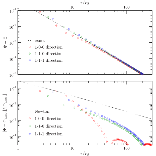
In order to compare the numerical results with the Schwarzschild solution, we write the Schwarzschild metric using so-called “isotropic coordinates” [39],
| (5.1) |
which, by comparing with eq. (2.1), gives following analytic expressions for the relativistic potentials as a function of the coordinate distance :
| (5.2) | ||||
| (5.3) |
Here, denotes the Schwarzschild radius, and we note in the Schwarzschild solution. We should also point out that, for the purpose of this comparison, we use Minkowski space as the background model since the entire simulation volume is in vacuum except for a single cell. In other words, we set which implies by eq. (2.6), and therefore we can set and identify .
It is instructive to expand the exact expressions for , which gives
| (5.4) | ||||
| (5.5) |
The Newtonian limit is given by the first term in this expansion, . The next weak field correction to this is suppressed by another power of , and so on. As is evident from Figure 1, our numerical scheme correctly accounts for the next-to-leading order terms, meaning that the errors are suppressed by an additional power of as compared to the Newtonian approximation. We note in passing that these are the terms relevant for the perihelion advance of Mercury. A similar study was presented in [40], where our framework is applied to a spherically symmetric setup.
We want to emphasize that the accuracy discussed here is a fundamental limitation of the weak field expansion which is independent of the discretization scheme. We expect our weak field approximation to break down at next-to-next-to-leading order (in the above expansion) even at infinite resolution. In practice, however, one has to deal with additional discretization errors. For the numerical test presented here we chose an extremely high resolution such that these effects are subdominant. This generally is not possible in many practical applications.
Figure 1 shows that our code models the space-time geometry around a Schwarzschild black hole correctly and with sub-percent precision for . In other words, our weak field limit is accurate as long as our resolution is larger than about 0.1 parsec, as the Schwarzschild radius of a black hole (about 5 times larger than the largest currently known black hole) is only about 0.01 pc. The same is not true for Newtonian codes as e.g. is identically zero in this approximation. Of course on such small scales many other effects that are currently neglected, like baryons, play an important role.
5.2 Code comparison with Gadget-2 and RAMSES
In order to test further some aspects of our implementation, in particular the particle-mesh scheme, we added the option to run simulations using Newton’s theory of gravity in our code. With this option, instead of the full stress-energy tensor, the code computes a Newtonian density contrast by particle-mesh projection of the rest-mass distribution. Then, a Newtonian potential is computed by solving
| (5.6) |
using Fourier analysis. Here is the average rest-mass density which, in a Newtonian setting, coincides with the background model for of matter. The algorithm used for eq. (5.6) is fundamentally very similar to the one which is used for solving eq. (2.9). Finally, for the geodesic equation we take the Newtonian limit where
| (5.7) | |||||
| (5.8) |
With these modifications the code therefore solves the Newtonian system of equations using essentially the same numerical techniques which we want to employ for the relativistic simulations. Of course the relativistic framework is much richer and needs several additional algorithms, but at least some parts of the implementation can now be compared to existing codes.
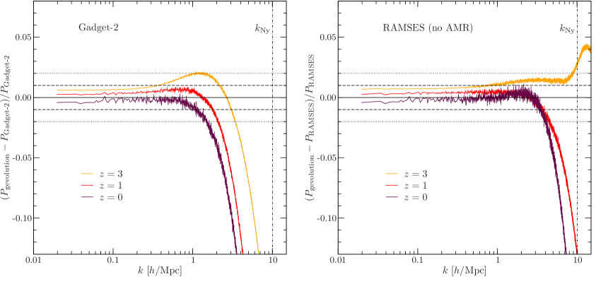
We choose to compare our implementation with Gadget-2 [41, 42] and with RAMSES (version 3.0) [43]. The numerical approach used in Gadget-2 is very different from ours, in particular with respect to the force computation at short distances. The agreement of the results hence is a good indication for the robustness of the N-body approach and allows to assess the detriment of working at fixed resolution. RAMSES on the other hand, like gevolution, uses a particle-mesh scheme but it can increase force resolution by performing adaptive mesh refinement. However, for our comparison we disable this feature, forcing the code to work at fixed resolution. This means we are looking at two cases: one where the numerical schemes are very different and one where they are quite similar (but still different).
We generate an initial particle configuration corresponding to a CDM cosmology888As explained in Appendix A the linear particle displacement for a Newtonian simulation differs from the one of Poisson gauge used for our relativistic simulations. This issue is taken into account when we generate initial data. which is then evolved by all three codes. Using identical initial data the comparison is not affected by cosmic variance. Figure 2 shows the relative difference of the power spectra after the codes have evolved the particle configuration from initial redshift to , , .
The left panel shows the comparison between Gadget-2 and gevolution. As may be expected, our code displays a significant deficit in power as one approaches the Nyqvist frequency. This is due to the fact that we work at fixed resolution. On scales well below the Nyqvist frequency, however, the results agree to within one percent, even in the nonlinear regime. It should be noted that an even better agreement would be hard to achieve since both codes employ a first-order-in-time integration scheme but are based on very different numerical approaches. In other words, the difference is roughly what one expects for two different integration methods (see also [44]).
The right panel shows the comparison between RAMSES and gevolution. As both simulations were run at the same fixed resolution the agreement is significantly better. However, the discretization schemes are slightly different, in particular concerning the force interpolation (RAMSES uses a five-point gradient) and the time integration (RAMSES works in “super-conformal time”). Because of the former there is no reason why the codes should agree as one approaches the Nyqvist frequency. The latter, on the other hand, may be responsible for the small constant offset at large scales which however remains within one percent.
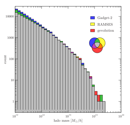
Figure 3 shows the comparison of the halo mass distributions of DM halos at redshift , extracted for the simulations using the Rockstar halo finder [45]. As expected from the preceding discussion, the agreement on the count of large-mass halos is very good, while gevolution shows a deficit of small-mass objects. Nevertheless, at the resolution used for this comparison, the halo abundance found with gevolution appears to be reliable over two orders of magnitude in mass.
The comparison shown in Figures 2 and 3 was based on simulations with particles and a comoving box of Mpc/, which results in a mass resolution of . The lattice in gevolution and RAMSES had points, whereas Gadget-2 used a lattice for computing the long-range forces and its tree algorithm for the short-range contributions. The latter allows Gadget-2 to resolve much smaller scales999Note, however, that there is no initial power beyond the Nyqvist frequency of the particle ensemble. and therefore requires significantly more work. We found that the simulation done with Gadget-2 consumed about seven times as many CPU-hours as the simulation done with our code, even though both codes integrated for roughly the same number of time steps. Restoring the relativistic setting some of this advantage is lost due to the additional work required for solving a more complicated geodesic equation. The additional metric components and are also computed and recorded in a Newtonian run of our code — they are just not used in the dynamics. For this reason we find that RAMSES (without adaptive mesh refinement) runs about twice as fast as gevolution. We nonetheless demonstrate that our relativistic scheme is not fundamentally much more expensive than a Newtonian one.
Having established good agreement with existing numerical codes when working in a Newtonian setting one can proceed to study all the aspects of the relativistic framework by internal comparison. In other words, by switching between the two theories of gravity (Newton and GR) within our code one can study the differences based on a single implementation without changing the systematics, the data format, or other collateral elements which complicate matters.
5.3 Background evolution
In order to provide further insight into the role of the background model, elucidating the reasoning of Section 2.1, we conduct following numerical study. Let us assume we want to simulate a cosmology with massive neutrinos where the neutrino phase space is sampled with the N-body method. While the details of such simulations are the topic of the next section, here we are only concerned with the background model. Of course the usual way to construct the background model would be to integrate over the unperturbed phase space distribution functions of the neutrino species in order to determine their background energy densities which enter Friedmann’s equation. This is, in fact, how the background model used in the next section is constructed. It is also the background model assumed by linear Boltzmann codes such as CAMB [46] or CLASS [47].
Let us compare this background model with an even simpler approximation where we completely ignore the kinetic energy of the neutrinos and only consider their rest mass contribution to the background. This is a good approximation as soon as the neutrinos are non-relativistic, but it leads to some noticeable differences at higher redshifts101010In the radiation dominated era this approximate background model would, in fact, be terribly wrong. However, here we want to use the approximate model only during N-body evolution, i.e. long after the end of radiation domination.. Since we argue that the choice of background model is to some extent arbitrary, we want to understand what happens if one uses this approximate background model in our N-body code.
As should be clear from the discussion in Section 2.1, the subtraction of an imperfect background model in eq. (2.7) leads to a homogeneous mode in this equation, i.e. to the appearance of a non-vanishing homogeneous mode in the scalar metric perturbations and . Let us denote this homogeneous mode as , and we remind the reader that we use our gauge freedom to set , which corresponds to a certain choice of global time coordinate . The spatially homogeneous part of the metric is then characterized by following line element:
| (5.9) |
Furthermore, the approximate background model has a certain conformal Hubble function determined by solving the Friedmann equation for that model, where .
Notice, however, that we can define the following renormalized scale factor and renormalized time coordinate , such that the new line element looks like an unperturbed Friedmann model,
| (5.10) |
up to higher-order corrections which we neglect in our weak-field expansion. The renormalized Hubble function is, to leading order in the weak-field expansion, related to the original one as
| (5.11) |
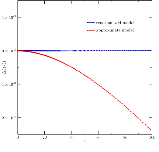
To summarize, the fact that we have adopted an approximate background model gives rise to a homogeneous mode which renormalizes the background. Figure 4 shows the relative change of the Hubble function for the approximate and the renormalized model, both with respect to the model where the neutrino energy densities are computed by integrating over the unperturbed distribution functions, i.e. the background model which is considered the usual one in linear perturbation theory. More specifically, , where is the conformal Hubble function obtained by solving the FLRW reference model exactly, including the relativistic energy densities of the neutrino species.
As one can see from Figure 4, the approximate model deviates noticeably from the reference model at high redshift since it misses the kinetic energy of the neutrinos which becomes gradually more important as one moves backwards in time. The renormalized model, on the other hand, coincides almost perfectly with the reference model. We also checked that the homogeneous mode , and therefore the renormalization, goes down to nearly zero as soon as we adopt the more accurate background model . Some tiny differences are expected due to the fact that beyond linear order there are some terms which do not average to zero in eq. (2.7) but which are not taken into account in the reference model. These are, in particular, the kinetic energy and binding energy of CDM perturbations [24]. However, in our example, these effects lead to a much smaller renormalization of the background than the neglect of the neutrino kinetic energy.
What we have demonstrated with this exercise is the following. The precise choice of background model is indeed not important in our framework. Any inaccuracy in the model is consistently accounted for when solving for the perturbations. In particular, the homogeneous mode in the scalar metric perturbations renormalizes the background model towards a unique solution which could be called the “resummed” background model from the point of view of our gauge choice. One should keep in mind, however, that we work in a weak field expansion, and therefore this renormalization scheme only works as long as the difference between the adopted model and the “resummed” one remains small. To make this statement more precise, we require at all times. In practice one can use the numerical value of as a diagnostic to determine whether the true geometry is adequately described by the adopted background model.
It should also be stressed that the traditional Newtonian approach neglects any possible renormalization of the background by construction. While it is possible to estimate the size of the error (see again [24]), it is not straightforward to correct for it within the course of the N-body evolution. The main reason is that Newtonian quantities, e.g. the density, are computed in an unperturbed geometry.
5.4 Neutrino cosmology
In this section we want to apply our relativistic N-body scheme to a cosmology with massive neutrinos. This is especially important as the effects of neutrinos on cosmological large scale clustering is one of the most promising paths to measure the presently unknown absolute mass scale of neutrinos and it is one of the main goals of several large scale surveys which are presently planned [48, 49, 7, 50]. The free streaming scale of neutrinos, , is given (very roughly) by the particle horizon at the time neutrinos become non-relativistic, i.e. when . Neutrino density fluctuations with wave numbers larger than are damped by the free streaming of neutrinos. As only neutrino fluctuations are damped, the amount of damping of the matter power spectrum depends on , which is also determined by the neutrino mass. Details on neutrino cosmology can be found in the monograph on the subject [51].
Here, we focus on two important effects. Firstly, the presence of a free streaming relativistic species (massive or not) gives rise to anisotropic stress (sometimes called shear) which is an important source for . In fact, as long as the neutrinos are relativistic, they are the dominant contribution to on scales larger than the free streaming scale . This is a relativistic effect which is not present in Newtonian N-body codes which only determine a Newtonian approximation to and set . The second effect comes from the fact that, as mentioned above, free streaming washes out density perturbations in the neutrino distribution. Massive neutrinos, which are non-relativistic at low redshift, form a component of the total matter power spectrum which is smoother than that of CDM. Therefore, at fixed total matter density (including massive neutrinos), a larger neutrino mass leads to a lower total matter power at small scales. This only affects scales below the free streaming scale . On scales much larger than that, the free streaming has little effect on the power spectrum.
The consistent treatment of neutrinos within N-body simulations constitutes a difficult problem which is the domain of an entire field of research, see [51] for an overview. The smoothness of the neutrino density field suggests that a perturbative calculation could lead quite far. For instance, one can use the linear solution of the neutrino perturbations computed with a Boltzmann code and add their contribution to the density field in Fourier space, see e.g. [52]. This method can be improved to take into account the potentials of nonlinearly evolved DM [53], however, it remains difficult to account for the phase information in the neutrino perturbations. In this perturbative formalism the neutrinos are treated as an independent, linear Gaussian random field and it fails to capture the full picture in the deeply nonlinear regime as the density contrast of neutrinos becomes larger than unity even for quite moderate neutrino masses.
Treating the neutrinos as N-body particles (see e.g. [34, 35]) seems conceptually straightforward and it should contain all the relevant physics. The main difficulty here is the fact that the initial phase space distribution is very broad: it is an extremely relativistic Fermi-Dirac distribution. This is true even in the non-relativistic regime at low redshift since neutrinos have decoupled while still relativistic and they cannot return to thermal equilibrium later due to their weak coupling. Sampling this distribution with N-body particles is very inefficient and shot noise becomes a serious concern (this problem is absent within the perturbative approaches mentioned earlier). We nevertheless follow this approach and try to address the problem of shot noise as good as we can.
5.4.1 Shot noise
We take two measures to mitigate shot noise. Firstly, we ensure that the power spectrum of the perturbations in the total energy density is not significantly affected by shot noise on any scale resolved by the simulation. This is possible even in cases where the neutrino density power spectrum is dominated by shot noise, as is the case on small scales and at high redshift when neutrinos are still relativistic. However, the neutrinos are only a small contribution to the total energy density, and it turns out that we can reduce their shot noise to a level well below the total matter perturbation power.
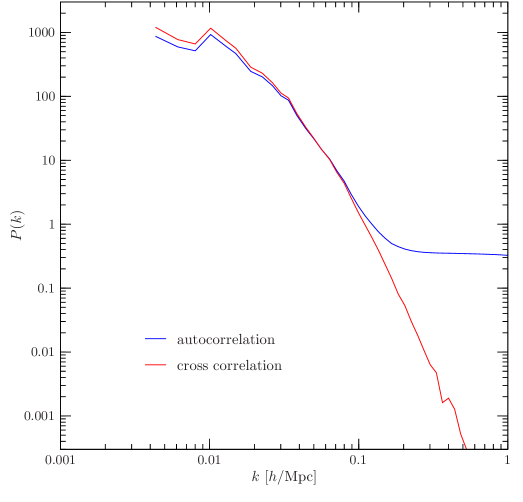
When computing the power spectrum of the neutrino density, and also the power spectra of any other quantity which linearly depends on the neutrino stress-energy, such as , we can use a trick to suppress the shot noise contribution [35]: we simply split the neutrino particle ensemble arbitrarily into two subensembles of equal particle number and then compute the cross-correlation power spectra between the two subensembles. Since both subensembles sample the same distribution, the cross-correlation is a good proxy for the autocorrelation. However, since the shot noise is uncorrelated between the subensembles, it partially cancels out, the degree of cancellation depending on the number of modes contributing to each bin. Schematically, denoting the full numerical density fluctuation by , the physical density contrast by and the shot noise by ,
| (5.12) | |||||
The split into two sub-ensembles gives two numerical amplitudes , , whose shot noise contributions are entirely uncorrelated. Figure 5 illustrates how effective this trick works in practice.
5.4.2 Simulation parameters and initial conditions
As example we choose a cosmology with three massive neutrino species, with mass eigenstates of eV, eV, and eV, respectively. This corresponds roughly to a normal hierarchy where we neglect the smaller of the two experimentally known mass-square differences. The remaining cosmological parameters are chosen compatible with current observations [54]. In particular, we set , , , (at Mpc-1), and . The value of is only used to convert the physical neutrino density to a dimensionless density parameter – by choice of appropriate units all other computations are independent of .
Since our code does not include a treatment of baryonic physics we treat CDM and baryons as a single species, ignoring the somewhat different clustering properties which are mostly important at small scales. The baryon acoustic oscillations in the linear power spectrum which are generated in the coupled baryon-photon fluid prior to recombination are contained in our initial conditions. However, late time baryonic effects in non-linear structure formation are not included. Photons are only taken into account at the background level, i.e. we neglect the perturbations in the radiation field. In the present treatment we also neglect primordial gravitational waves. These remain small contributions to the curvature at all times and can be calculated to sufficient accuracy within linear perturbation theory. Since they are uncorrelated with scalar perturbations, where it does not vanish, their effect can be simply added to the statistical quantities computed here, like e.g. the tensor perturbation spectrum.
To set up initial conditions we follow a procedure proposed in [36]. Using a Boltzmann code [47], we compute the linear solutions (as a function of time) of perturbation modes, covering the entire range of scales represented in our simulation. Next, we initialize the particle ensemble at redshift , at which time the comoving particle horizon is just below our lattice resolution and all modes in the simulation are superhorizon. At this time we may assume that the perturbations are adiabatic and Gaussian. With this assumption, we draw a realization for which also determines the initial particle positions, as well as the initial values for . The amplitudes are determined from the linear mode functions using cubic spline interpolation in Fourier space. A random momentum is added to the neutrino particles according to the initial Fermi-Dirac distribution. Details are given in Appendix A.
The phase space of the N-body ensemble is then evolved to the initial redshift of the N-body simulation, which was chosen as . This is done by evolving each perturbation mode of the potentials and according to the linear solution, and then solving the geodesic equation for the particles in these potentials. While this is a computationally expensive111111About of the computational time was spent pre-evolving the particles from to . The remaining were attributed to the fully nonlinear N-body simulation from to . way to set up the initial particle phase space, it guarantees that all moments of the distribution function and all relative phases are set up correctly, at least in principle. One may argue that much of this information is swamped by shot noise, but this depends on the number of particles in the simulation. Our largest simulations had a lattice of cells and a total of billion neutrino particles and billion CDM particles. The box size for this simulation was chosen as Mpc/, giving a resolution of Mpc/. The integration used time steps: steps for pre-evolving the particle phase space in the linear potentials and steps for the nonlinear evolution. The entire simulation used some CPU hours on the Cray XC30 supercomputer Piz Daint.
In addition to a simulation with massive neutrinos we also do a simulation for the massless case. In this case the neutrinos are simply treated as part of the radiation field, with the standard value of . The density of CDM is increased to in order to have the same total matter density in both simulations (at ). All other simulation parameters are kept unchanged, in order to minimize systematics.
5.4.3 Numerical results
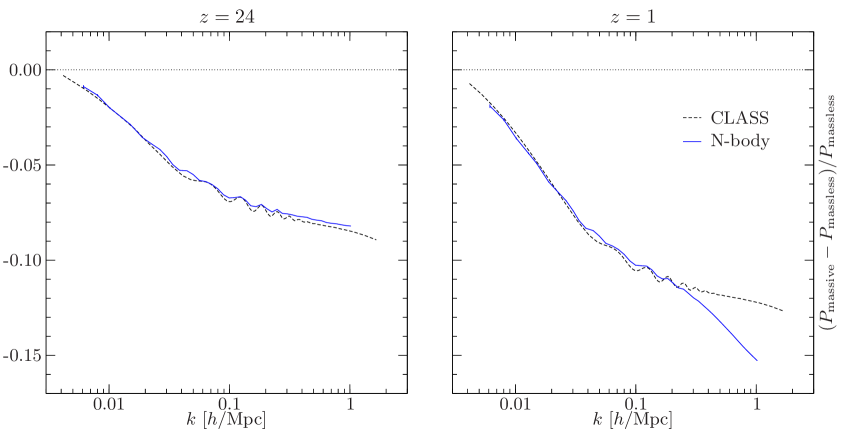
Figure 6 shows the relative difference in the perturbation power spectrum of between the case of massive and the case of massless neutrinos. The dashed line indicates the prediction in linear perturbation theory, obtained with the Boltzmann code CLASS. Our numerical results are in good agreement with the linear calculation in the regime where we expect the latter to be valid. At late time and on small scales the linear theory breaks down, and we see that the suppression of power in this regime is enhanced by nonlinear effects. This is quite intuitive: in the massless model the power is higher, the modes become nonlinear quicker and hence have more time to increase their power through nonlinear growth.
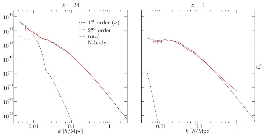
As is well known, any free streaming relativistic species gives rise to anisotropic stress which sources even at the linear level, see e.g. [55]. At second order also nonrelativistic species and even geometry contribute, the latter by virtue of the nonlinear terms in the weak field expansion of the Einstein tensor, see eq. (2.10). Figure 7 shows the numerical power spectrum of at two different redshifts. We also indicate the contribution of the neutrino shear stress as computed in linear perturbation theory, as well as the second order contribution from CDM and geometry. The radiation field also has some anisotropic stress, but it is subdominant at these redshifts. We remind the reader that perturbations in the radiation field are neglected in the simulation.
At the neutrino shear stress is still the dominant contribution to at large scales /Mpc, while the second order contributions from CDM and geometry dominate at smaller scales. Later, at , the neutrino shear stress has decayed due to further redshifting of the neutrino distribution. At the smallest scales, /Mpc, the power spectrum of gets enhanced due to nonlinear evolution, an effect that is missed in the perturbative calculation which only goes to second order.

Figure 8 shows a Mpc/ region around a massive cluster at . As is evident from the right panel, the neutrinos form a very smooth component of the matter distribution. Only the most massive objects are able to truly bind the neutrinos within their potential wells. One should keep in mind that the mean thermal velocity for a eV neutrino is about km/s at , more than the escape velocity of most small scale structures.
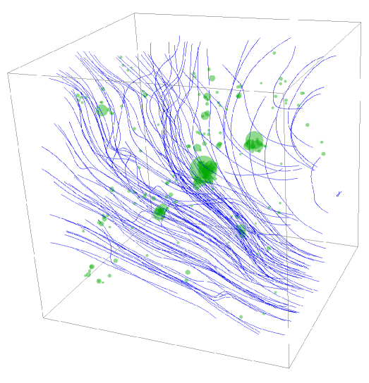
A three-dimensional rendering of the same region is shown in Figure 9 where we also include a stream plot of the curl of the spin-1 metric component, . Here we note that at leading post-Newtonian order (i.e. at lowest order in inverse powers of the speed of light) the frame dragging force is given by a term in the geodesic equation, see e.g. [19]. Therefore the curl of plays a role analogous to the one of the magnetic field in the Lorentz force (while the gradient of is analogous to the electric field). The magnitude of in the particular volume shown in Figure 9 is of the order of /s in proper units. Due to the equivalence principle all nonrelativistic matter gyrates at this frequency. However, the corresponding period is five orders of magnitude larger than the present age of the Universe.
5.4.4 Newtonian and relativistic particle trajectories
In order to challenge the Newtonian approach used in traditional N-body codes we did a few smaller simulations using the Newtonian equations of motion (5.7), (5.8) for the particle update of the neutrinos. While this approximation introduces large errors on individual particle trajectories, the impact on expectation values (such as the power spectrum) seems to be quite small. However, at early times the Newtonian propagation does not respect causality, as the velocity of some particles becomes much larger than the speed of light. We therefore expect some errors to appear at the free streaming scale .
If we define precisely as the mean comoving distance covered by a neutrino particle between the big bang () and today (), one finds that for mass eigenstates of eV and eV the corresponding relativistic free streaming scales are Mpc/ and Mpc/, respectively. Switching to the Newtonian approximation at some initial redshift changes these numbers somewhat. For an initial redshift of the apparent free streaming length increases to Mpc/ and Mpc/ for those neutrino masses, a respective change of and . The change is larger the smaller the neutrino mass and the earlier one chooses the initial redshift for the Newtonian evolution. It is quite possible that percent errors on the free streaming length may propagate into the results of high-precision Newtonian simulations, but a thorough investigation of this issue is left for future work.
We also note that the large distances travelled by the “superluminal” particles forces the Newtonian scheme to use a smaller time step. However, we think that all these issues can easily be mitigated by making use of the relativistic equations of motion. For any Newtonian code simulating neutrinos we therefore propose to use what we may call, somewhat imprecisely, “Newtonian gravity with special relativity.” By this we mean that we maintain the Poisson equation (5.6) which determines the Newtonian gravitational potential, but we change the equations of motion (5.7), (5.8) to
| (5.13) | |||||
| (5.14) |
which are approximations to the geodesic equations (3.4), (3.5) that are however valid at all orders in the velocity. Note the factor in front of the term which ensures the correct extremely relativistic limit: massless particles are deflected by which in the Newtonian limit is simply .
In this way it is guaranteed that the propagation of particles is causal, the free streaming length is computed accurately, and even the deflection of relativistic “test particles” by local potentials is treated correctly up to subleading weak field corrections. The above equations can easily be implemented in Newtonian N-body codes, even those which use tree algorithms that are based on two-body forces.
6 Summary
In this paper we have presented in detail our new, publicly available relativistic N-body code. In a previously published letter [19] we have shown the results for the relativistic degrees of freedom of the gravitational field, in particular frame dragging and gravitational waves. Here we explain in detail the theoretical underpinnings of the code, the approximation scheme used in our approach and the code structure. The details of the implementation of initial conditions, the particle to mesh projection and force interpolation as well as the Fourier space solver of the Einstein equations are presented in three appendices. The source files and a manual are available on a public Git repository:
After studying this paper we hope that people working in the field should be able not only to run the present version, but also to modify it for all interesting purposes like for studying models with dynamical dark energy or with modified gravity. The code is distributed under a free software license and we encourage everyone to share their developments with the community.
In order to validate the code we perform two numerical tests. First we compare with an analytic solution by computing the metric of a single point mass. We find that it fares considerably better than the Newtonian solution and correctly includes also the terms in the Schwarzschild metric which are of order and which are not present in a Newtonian approach. Our implementation of the particle-mesh scheme is further validated using a Newtonian setting where we can compare to existing N-body codes. Comparing to a simulation carried out with Gadget-2 we find that for a CDM universe the power spectra of density perturbations agree within 1% on scales larger than 10 times the Nyqvist frequency and within 2% for scales larger than 5 times the Nyqvist frequency down to redshift . Our code runs faster than Gadget-2, but of course being a pure particle-mesh code based on field theory, it cannot resolve scales smaller than the grid spacing. Gadget-2, on the other hand, follows the nonlinear evolution also on scales smaller than the Nyqvist frequency of its initial particle distribution.
In order to disentangle this resolution effect from other numerical differences we also compare to a simulation which was carried out with RAMSES at fixed spatial resolution, i.e. without using the adaptive mesh refinement capability of that Newtonian N-body code. In this case the agreement remains within 1% up to scales 3 times the Nyqvist frequency. As one approaches even closer to the Nyqvist frequency one expects that differences in the discretization scheme become increasingly relevant.
Thanks to the highly scalable latfield2 library [37] gevolution runs efficiently on the largest supercomputers with tens to hundreds of thousands of processor cores and supports very large grid sizes. Our relativistic code is therefore suitable especially on large to intermediate scales. On scales below Mpc/ the modelling of structure formation is probably limited by our understanding of baryonic physics rather than by relativistic effects.
As opposed to Newtonian simulations where the Hubble function is an external input and dissociated from the simulation dynamics, our relativistic approach jointly solves for background and perturbations in a self-consistent manner. We demonstrate numerically that small changes in the background model are automatically accounted for by the perturbations, leading to a unique “resummed” geometry which is independent of the arbitrary split between background model and perturbations. This renormalization procedure works as long as the assumed background model remains perturbatively close to the “resummed” one, a requirement which can easily be diagnosed by monitoring the homogeneous mode of the scalar metric perturbation.
We finally show first results obtained with our code for a cosmology with massive neutrinos. Contrary to other procedures used in the literature, which are based on Newtonian N-body codes, we treat the neutrinos fully relativistically and in a fully non-linear way from the beginning. We calculate which is dominated by free streaming neutrinos at early times and on large scales. Especially at late times we find no striking differences of our relativistic neutrino simulations compared to the Newtonian ones, but a detailed comparison is non-trivial and has to be presented in a future project.
Acknowledgments
We thank C. Fidler, M. Gosenca, S. Hotchkiss, C. Rampf, R. Teyssier, T. Tram and F. Villaescusa-Navarro for discussions. The numerical simulations were carried out on Piz Daint at the Swiss National Supercomputing Centre (CSCS). This work was supported by the CSCS under project ID d45, and by the Swiss National Science Foundation.
Appendix A Initial conditions
The general procedure for setting up initial data for a simulation is as follows. First, one chooses an initial time at which perturbation theory is still valid. This allows to make the connection with “initial” conditions set at the hot big bang using perturbative methods and known physics. These “initial” conditions are well constrained by observations of the cosmic microwave background. In this appendix, we explain how initial data for non-interacting particle species (relativistic or not) can be constructed in linear theory. The construction can be improved by including higher orders in the perturbation series, but this is beyond the scope of this paper. We also do not provide a discussion of additional sources here, such as scalar fields. For every particular model with new ingredients, one has to consider initial conditions appropriately. For the purpose of this work, we assume that it is sufficient to compute the initial perturbation amplitudes using a linear Boltzmann code such as CAMB or CLASS. The output power spectra of such a code are the input we need in order to generate a realization in terms of metric perturbations and the particle phase space distribution.
It should be stressed that the generation of initial conditions for our relativistic scheme, even though it follows similar procedures, is not identical to the Newtonian case. This is partially owed to the fact that gauge issues have to be considered and treated properly. Furthermore, our scheme is more complete in several respects. For instance, it is straightforward to take into account the fact that the potentials have a decaying mode originating from the transition between radiation and matter domination. The presence of the radiation era has a noticeable effect at high redshifts, , which is notoriously difficult to treat within a Newtonian N-body scheme. Our new framework is designed in order to take care of precisely such relativistic aspects.121212The anisotropic stress due to perturbations in the radiation field, especially for relativistic neutrinos, causes a mismatch between and at the percent level even in linear theory for and scales Gpc. Since and both correspond to first-order gauge-invariant quantities this effect is present in any gauge and can only be treated correctly if the two potentials are kept independent. While this is the case in our framework, the current implementation still ignores perturbations in the radiation field. Therefore the potentials inevitably still fail to match the ones computed with a linear Boltzmann code. This shortcoming could be overcome in the future, for instance by adding the linear perturbations of radiation to the N-body scheme.
The particle positions are generated by the action of a linear displacement field on a homogeneous “template”. In the simplest case, the template can be a regular arrangement of N-body particles similar to a crystal, but one could also use a template more similar to a glass, for instance. The displacement field corresponding to a particular realization of the density perturbation can always131313Since linear curl-type displacements do not change the density, this is true in linear theory even in the case where vector modes are present. The presence of vector modes would only affect the initial velocities. be written as a gradient, , which can be worked out from the linearized version of eq. (2.9),
| (A.1) |
where we introduce , and is the corresponding density parameter, . We follow the notation of [56].
To simplify the discussion, let us assume that one can separate all particle species into two classes at the initial redshift of the simulation, one where is a good approximation and one with . If a species is at the transition from being ultra-relativistic to non-relativistic, the initial redshift can be chosen differently in order to avoid this situation. Inspecting eq. (3.2) it is easy to see141414A simple way to see this is to go to the continuum limit where the sum over particles can be replaced by an integral over the initial particle positions. The “” arises as the Jacobian when changing the integral measure from – where the distribution in position space is uniform – to . See also [40]. that for nonrelativistic species, ,
| (A.2) |
For relativistic species there are various ways to implement a given density perturbation since the energy density depends on both, the number density and the particle momenta at leading order. The simplest setting is the one where the phase space distribution is thermal, in which case the number density and momenta are uniquely given by a temperature. In this case one finds
| (A.3) |
and a perturbation is added to the temperature in order to determine the thermal momentum distribution. Incidentally, in the case of adiabatic initial conditions where ], the displacement field for all particle species (relativistic or not) is given by the same scalar field . Here, the equation of state for nonrelativistic species, whereas for particles that are ultra-relativistic. We assume adiabatic initial conditions from now on, such that eq. (A.1) in Fourier space becomes
| (A.4) |
If and are Gaussian random fields, then so is , and its amplitude (rms value) can be obtained from the above equation as a function of the initial amplitudes of and , their deterministic mode evolution, and the known time-dependent background functions , and .
If adiabaticity is not a good approximation, for instance on sub-horizon scales for species which evolve differently after horizon entry of the modes, the displacement field is not given by a relation as in eq. (A.4). In general, each species has its own displacement field, related to its density perturbation according to eq. (A.2) or eq. (A.3). The displacement fields can therefore be constructed using the respective transfer functions computed with a linear Boltzmann code. Note that these transfer functions are often computed in the comoving synchronous gauge whose density perturbation is related to in Fourier space as
| (A.5) |
where the scalar velocity potential will be introduced below.
This concludes the discussion of the initial particle displacement. To summarize, the initial condition generator implemented in gevolution generates a Gaussian realization of according to eq. (A.4) using the output of a linear Boltzmann code, and the displacement acts on a given homogeneous template. Mode by mode this also determines the initial amplitude of and corresponding to this particular realization. In the remaining part of this appendix we discuss how to set initial momenta.
In general, the momenta for an ensemble of particles are given by a phase space distribution function. Even in cases where this function takes a simple form to begin with, its evolution can become very complicated which is the whole point of N-body simulations. For the purpose of setting initial conditions we however assume that the phase space distribution is determined to a good approximation by its first two moments. These are essentially given by the density, , and the momentum flux, , and we assume that the anisotropic stress (the traceless part of ) can be neglected. This situation is often compared to a perfect fluid which is locally described by its density and velocity fields.
We should stress that this so-called fluid approximation is a very restrictive assumption. While the stress-energy tensor can be constructed for any phase space distribution function by means of eqs. (3.2)–(3.10), the inverse is only possible in very special cases. We discuss two distinct cases here. In the first case, which is the one relevant for non-relativistic species, the momentum flux of the particle flow is much larger than the momentum dispersion. This means that the phase space distribution function is essentially a Dirac delta function in momentum space. In this case we do not care about the momentum dispersion, and the phase space distribution function can be sampled with a single particle whose momentum is set by the momentum flux of the flow.
In the second case, relevant for ultra-relativistic species, the momentum flux is generally much smaller than the momentum dispersion. The peculiar momenta are therefore dynamically important as they give rise, for instance, to a sound horizon and an effective pressure which even affects the background. The distribution of momenta is very broad and can certainly not be approximated by a delta function. For the purpose of setting initial conditions, we assume that the distribution takes a simple parametric form. In particular, the momentum flux is realized by displacing an isotropic distribution by an appropriate momentum vector in momentum space. An example would be a thermal momentum distribution which is boosted into a frame to match the desired momentum flux.
In order to be more specific, let us discuss again the situation where the perturbations of stress-energy are generated by a mixture of relativistic and non-relativistic species. We define a scalar potential for each species which characterizes the curl-free part of the momentum flux as151515Another frequently used quantity is the divergence of the velocity field, characterized by which is given by in Fourier space, cf. [55]. Note also that [56] uses yet another quantity denoted as and related to as . The motivation for this definition is that is dimensionless. However, we prefer to work with since it is related to the velocity field (in configuration space) by a local operation.
| (A.6) |
In the linear regime the curl part can usually be neglected. Furthermore, for adiabatic initial conditions the potentials defined in this way are identical for all species. We can therefore sum over all species and read off the potential from eq. (2.11),
| (A.7) |
By considering eqs. (3.2) and (3.10) this allows us to immediately set the initial momenta for non-relativistic N-body particles as
| (A.8) |
Note that the momentum depends on the mass of the N-body particle which is a simulation parameter without any physical significance. The code therefore internally works with the dimensionless quantity .
The momenta of relativistic particles, however, are given by a large stochastic component with a simple parametric, isotropic distribution and a comparatively small deterministic component which sets the mean momentum vector to
| (A.9) |
where denotes a (mass-weighted) mean over the particle distribution at fixed position. The main difference to eq. (A.8) is the fact that the momentum flux is realized in an average sense, and that the individual momenta can be vastly different from this average. The last term on the right hand side is the mean energy per particle (in the ultra-relativistic limit).
Adhering to the N-body concept, we model the phase space distribution by a large number of particles whose momenta are randomly drawn from the distribution function. However, the number of particles is limited by computational resources and therefore the sampling of phase space is generally very sparse. In our simulation reported in Section 5.4, we admit 5 neutrinos per lattice site, each with momentum , where is randomly sampling the momentum distribution and is typically much larger than . For a broad distribution (like the extremely relativistic Fermi-Dirac distribution of cosmic neutrinos) shot noise becomes a serious issue. In the power spectra we can reduce the noise significantly by cross-correlating neutrinos from two sub-ensembles which sample the same distribution. Furthermore, the relativistic species give a subdominant contribution to the energy density, so that the imprint of the noise onto the gravitational potential is negligible.
Note again that eq. (A.7) assumes adiabaticity; in situations where this assumption is dropped one can instead employ eq. (A.6) directly, using the transfer functions of as computed for each species separately. For non-relativistic species this equation implies
| (A.10) |
whereas the ultra-relativistic limit reads
| (A.11) |
Appendix B Particle-to-mesh projection and force interpolation
In any particle-mesh N-body scheme there are two different concepts for the representation of simulation data. One set of data represents a phase space distribution. It is most conveniently discretized by sampling it with N-body particles. The particle ensemble is stored as a list with six real-valued phase space coordinates per particle, the position and the momenta of the particles. Hence particles do not sit on the lattice sites. These coordinates are real-valued in order to allow for smooth particle trajectories. Another set of data represents fields. Such data is most conveniently discretized by sampling the field values on a discrete lattice which spans the three-dimensional simulation volume.
In order to couple the evolution of fields to the evolution of particles (and vice versa), one needs to provide methods which connect the two different ways the data is represented. This is achieved by two types of operations which are dual to one another. The particle-to-mesh projection converts some information contained in the particle ensemble into fields. In a Newtonian code one would, for instance, compute a density field from a given particle distribution. In our relativistic framework the quantity of interest is the stress-energy tensor of the particle ensemble. The dual operation is often called force interpolation because the Newtonian force on each particle is determined by interpolation of the gravitational potential to the particle position. We adhere to this terminology even though interpolation is not only used for forces, but any time we need to determine the value of a field at the position of a particle.
A systematic way to construct these operations can be found in textbooks, e.g. [57]. For our purpose it is useful to define two one-dimensional weight functions,
| (B.1) |
and
| (B.2) |
where denotes the lattice unit, i.e. the coordinate distance between neighboring lattice points. The utility of these weight functions becomes evident when considering the respective constructions of a (one-dimensional) density field,
| (B.3) | |||||
| (B.4) |
where and are the mass and position of the th particle, and is a discrete index labelling the lattice points. The subscript NGP refers to nearest grid point assignment since using the weight function corresponds to assigning all the mass of a particle to the nearest lattice point. This is often considered the zeroth-order approximation to the density field. CIC stands for cloud-in-cell, and the weight function corresponds to distributing the mass of a particle between the two neighboring lattice points in such a way that the mass assignment changes linearly with the particle position. Higher order assignment schemes can be constructed but we do not discuss them here.
The weight functions also naturally define corresponding interpolation operations,
| (B.5) | |||||
| (B.6) |
Note that the sum is now performed over the lattice points.
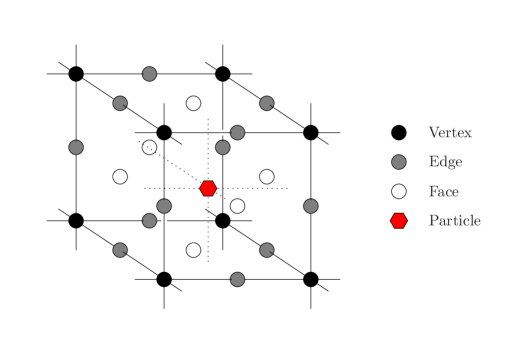
Another aspect of the lattice discretization concerns the definition of discrete derivative operators. Here we always employ the one-sided two-point gradient, which in one dimension is defined as
| (B.7) |
Note that this type of gradient would naturally be associated with a lattice which is shifted by half a lattice unit. The three dimensional generalization of this gradient operator has the three components of the gradient being associated with three different shifted lattices, as the shift always applies in the direction in which the derivative is taken.
We apply this prescription to all vector-valued fields. Figure 10 shows a sketch of a lattice cell indicating the various locations to which field values can be associated. All scalar fields are associated with the vertices of the primary lattice. The components of a vector field are associated to the edges connecting the vertices, each possible orientation of the edges corresponding to one component of the vector. Note that this convention ensures that the divergence of a vector field – which is a scalar – is again associated with the vertices if one uses our discrete choice of derivative operator. Finally, the off-diagonal elements of a tensor field are associated to the faces of the lattice cell, while the diagonal components are represented once more at the vertices. This ensures again the compatibility with our previous conventions when constructing vectors or scalars by applying discrete derivative operations on a tensor field (and vice versa). Note also that the curl acting on a vector field associated with the edges gives a result which is naturally associated with the faces, and vice versa. This is due to the fact that the curl of a vector is truly an anti-symmetric tensor, , which only in 3 dimensions can be represented as a (pseudo-)vector. A double curl does not change the association with lattice sites, and neither does the gradient acting on a divergence.
Let us now turn back to the problem of particle-mesh projection and force interpolation. In order to construct a scalar quantity (like the rest-mass density in a Newtonian setting or, for instance, in our framework) from an N-body ensemble we employ the three-dimensional version of the CIC operation. This means that we evaluate eq. (3.2) at the lattice points by replacing
| (B.8) |
in that equation. Here and in the following, , , are the discrete indices labelling the vertices of the three dimensional lattice. The geometric corrections brought by the -dependent terms in eq. (3.2) are incorporated by evaluating directly at the lattice points161616This choice is arbitrary and other choices lead to different discretization errors. As the geometric corrections themselves are small we are not so much interested in the discretization error on them, and therefore make a choice based on convenience of implementation.. In Newtonian theory these corrections are not present and essentially reduces to the CIC rest-mass density.
One could, of course, proceed with the same prescription also for the construction of vector or tensor fields. However, we adhere to a somewhat different construction principle. We require that the projection and interpolation operations for each particle only depend on the lattice quantities which are associated with the boundaries of the lattice cell containing the particle. These are the quantities associated with the eight vertices, the twelve edges and the six faces belonging to that cell (see Figure 10).
The vector projector used to construct is obtained by replacing
| (B.9) |
in eq. (3.10) for the component which is associated with the lattice edge sites , and analogous replacements for the other two vector components. This assignment scheme is a mixture between the NGP and CIC method. Observing that
| (B.10) |
reveals a special property of this assignment scheme. Namely, if the rest-mass density is constructed on the lattice using CIC assignment, and the momentum field is constructed using the vector projection above, the continuity equation
| (B.11) |
is satisfied identically on the lattice with our definition of the discrete divergence operator. The general relativistic counterpart to this equation is the time component of the covariant conservation equation,
| (B.12) |
At zeroth order in the metric perturbations the only non-vanishing Christoffel symbols are , and . To satisfy eq. (B.12) at zeroth order exactly when using the CIC assignment scheme (B.8) for , one not only has to choose the assignment (B.9) for the vector field : interestingly, the CIC assignment scheme (B.8) has to be chosen also for the diagonal components of .
What about the off-diagonal elements of ? Looking at the spatial part of the covariant conservation equation,
| (B.13) |
again at the zeroth order, one finds that the best choice seems to be the replacement
| (B.14) |
in eq. (3.2) to compute the projection for at the lattice face , and analogous expressions for the other off-diagonal elements. This choice ensures that the contributions to eq. (B.13) from the off-diagonal quantities cancel exactly with corresponding terms coming from . Unfortunately there remains a residual coming from the one diagonal term of which contributes to this equation. It seems difficult to satisfy the condition which makes this residual vanish, in particular if one wants to maintain also eq. (B.12). The same problem is already present in the Newtonian framework if one considers the Euler equation which is the nonrelativistic counterpart of eq. (B.13). At the present stage this remains an artefact of the lattice discretization that we have to bear with.
To summarize, with the choices of projection operations given above, the following coherent picture emerges. The contributions of each N-body particle to the stress-energy tensor are projected onto lattice sites belonging to the cell in which the particle resides (see Figure 10). For components associated with the vertices of the lattice, such as and the diagonal elements of , the projection weights for the eight relevant vertices are piecewise trilinear functions of the three particle coordinates, corresponding to a three-dimensional CIC assignment. For components associated with edges of the lattice, such as and , the projection weights for the four relevant edges (per vector component) are given by piecewise bilinear functions of the two particle coordinates orthogonal to the edge direction, corresponding to a two-dimensional CIC assignment. Along the coordinate of the edge direction the weights are piecewise constant as in the NGP assignment. Finally, for components associated with the faces of the lattice, such as the off-diagonal elements of , the projection weights are piecewise linear functions of the particle coordinate orthogonal to the face plane, corresponding to a one-dimensional CIC assignment. Along the other two coordinates the weights are piecewise constant. Discretization errors are absent in eq. (B.12) and minimal (in some sense) in eq. (B.13), at zeroth order in the metric perturbations171717At first order in the metric perturbations the discretization errors depend on the way one chooses to evaluate the first-order contributions to the Christoffel symbols as well as on various other choices (see also footnote 16). They are therefore not a property of the particle-to-mesh projection alone..
Our force interpolation is simply the dual of this prescription. For instance, in order to evaluate a vector field at a location inside a lattice cell, the values specified on the edge sites of that cell are interpolated using the bilinear weights of the two-dimensional CIC assignment. In short, the interpolation amounts to an appropriately weighted average of the field values present at sites on the boundary of the cell.
Appendix C Fourier-space solvers for Einstein’s equations
In this appendix we explain the numerical algorithms implemented in our code for solving eqs. (2.9) and (2.10) in order to determine the metric perturbations , , and on the lattice. Let us begin with eq. (2.9) which is a nonlinear parabolic (diffusion-type) equation for . We employ a first-order in time solution strategy, which allows us to effectively decouple the equation from the other set of Einstein’s equations at each update step. This is because we can choose to evaluate the -dependent term at the initial time where it is already known. In order to ensure unconditional stability of the solution strategy, we have to use an implicit method (see [58] for more details). In the following, we label the time steps by a discrete index and the lattice points again by discrete indices , , . The finite difference between time steps are denoted as , and the lattice unit is denoted as as before. Let us also introduce the shorthand . With these conventions, we can write a finite-difference version of eq. (2.9) as
| (C.1) |
where we have divided out a factor to move it to the right hand side. The implicit character of this finite-difference equation comes from the prescription to evaluate the discrete Laplace operator at the final time . Had we chosen to evaluate it at instead, we would obtain an explicit equation which could be solved for immediately. However, this strategy would impose a condition on in order to maintain stability. This so-called Courant-Friedrichs-Lewy condition requires that information may not travel farther than one lattice unit in each update, i.e. . Such a requirement would render high-resolution simulations prohibitively expensive.
Once we have ensured stability, the choice of when to evaluate any of the remaining terms is not important in a first-order scheme. For convenience, we evaluate the stress-energy tensor at but we compute the geometric corrections using the values of the perturbations at . Also the remaining terms on the left hand side are evaluated at . In a second-order in time integration scheme these choices would have to be modified, and all the evolution equations would have to be solved concurrently (for instance, would occur in the above equation as well). This could be achieved using a predictor-corrector method, but we do not discuss this here since a first-order in time scheme is sufficient for our purpose. Note also that the Poisson equation used to compute the Newtonian potential would effectively be solved using a zeroth-order (in time) scheme, as time derivatives do not occur in this approximation at all.
In order to solve eq. (C.1), the code collects all the known terms, i.e. the stress-energy tensor and the terms built with known field values (those at ), and combines them to a single (nonperturbative) source field ,
| (C.2) |
With this definition, the unknown field values of at are given implicitly by
| (C.3) |
Note that this equation is linear in the unknown field values, and we can therefore invert the finite-difference operator on the left hand side using Fourier analysis181818Numerically this may not be the most efficient approach. For instance, the so-called multigrid algorithm is known to be superior in many cases and can even be generalized in order to invert nonlinear operators. In our previous work [27] we considered yet a different algorithm based on an operator splitting method that performs an approximate inversion. It turned out that, once the symmetry assumption used in that work was dropped, the errors introduced by this approach were intolerable in practice. We decided to use Fourier analysis (which is an exact method) because we use a similar solution strategy for eq. (2.10). The latter requires more execution time than eq. (2.9) in any case, and optimizing on eq. (2.9) would therefore not have a large impact on total performance.. The discrete Fourier transform
| (C.4) |
is computed using a distributed three dimensional FFT algorithm provided by the latfield2 library. Here, , , are discrete indices labelling the Fourier wave vector and denotes the number of lattice points in each dimension, the total lattice having points. In discrete Fourier space eq. (C.3) becomes
| (C.5) |
As usual, the linear finite-difference operator in position space corresponds to a multiplicative function which depends on the Fourier wave vector. We can now simply solve this algebraic equation for and perform the inverse FFT in order to obtain . At this point it is important to note that the equation gives a meaningful value also for at . In other words, if has a homogeneous mode it sources a homogeneous mode in . This property is crucial for internal consistency of the scheme. In the Newtonian limit, does not have a homogeneous mode by construction, and it is hence consistent to set the homogeneous mode of to zero.
Next, we have to solve for the remaining perturbation variables , and ; we follow a very similar philosophy. We construct a nonperturbative source tensor by moving the nonlinear terms of eq. (2.10) to the right hand side. As explained in Appendix B, scalar quantities like and are represented at the vertices of the lattice, as are the diagonal components of spatial tensors, e.g. . The components of are represented on the edges, and the off-diagonal elements of a spatial tensor on the faces of the lattice, respectively. This needs to be taken into account when constructing the source tensor . In order to avoid too many messy equations, we give the construction of one diagonal element, , and one off-diagonal element, . The other components of the tensor are constructed analogously.
| (C.6) |
| (C.7) |
We have written eq. (C.7) in a suggestive way such that the terms can be easily identified. For instance, the second line is the product with the two gradients interpolated to the face of the lattice cell at . Within the code though, these expressions are rearranged in order to minimize the number of operations required to construct . Note also that the terms proportional to in eqs. (C.6) and (C.7) are neglected in the public version of the code. This is done for efficiency reasons and is justified as long as , since only appears in the combination within these equations.
With , the continuum version of eq. (2.10) reads
| (C.8) |
which is linear in the unknown perturbation variables191919The dependence of on these variables is very subleading and for the purpose of solving this equation we simply estimate their contributions using the values from the previous time step. This is fine within a first-order in time integration scheme as the one we use here. If one were to move to a higher-order scheme, one could again employ a predictor-corrector method. , and , meaning that we can again use Fourier analysis as a solution strategy. There is a great advantage to this approach: in Fourier space, the separation into spin-0, spin-1, and spin-2 components is straightforward.
For the spin-0 component, we simply contract the indices with two Fourier wave vectors. The gauge conditions then imply that
| (C.9) |
The spin-1 component is projected out by applying the transverse projector on one of the indices and contracting the other one again with a Fourier wave vector. We obtain
| (C.10) |
Finally, for the spin-2 projection, we apply , which yields
| (C.11) |
The equations (C.9), (C.10) and (C.11) are valid in the continuum limit where the Fourier wave vectors correspond to spatial derivatives in position space. On the lattice, we have to replace these wave vectors by the algebraic expressions corresponding to the specific notion of finite-difference operators chosen in the discretization procedure. For instance, one can find a version of acting in discrete Fourier space in such a way that, after inverse Fourier transform, the discrete divergence of vanishes exactly, satisfying the discrete version of the gauge condition.
Explicitly, we define the discrete Fourier components of as
| (C.12) | ||||
| (C.13) |
and similarly for the remaining components. Note that the off-diagonal elements are defined with a phase factor which accounts for the fact that these components exist on the faces of the lattice cells and not on the vertices. Let us also define a lattice momentum as
| (C.14) |
With these definitions, the discrete versions of eqs. (C.9) – (C.11) are simply given by replacing , , , and so forth. The discrete Fourier transform of is defined in the same way as the one for , while the one for takes the form
| (C.15) |
and similarly for the other components, taking into account the fact that the components of a vector reside on the edges of the lattice cells.
In order to evolve , the code keeps a copy of in Fourier space. According to eq. (C.10), the update step for is then performed as
| (C.16) |
Even though we have all the ingredients ready for solving eq. (C.11), in the present version of the code this is not what we do. The reason is that, for the scenarios studied in this work, the scattering of particles with the spin-2 metric perturbation is a very small effect and is therefore neglected. The effect is much smaller than the frame dragging caused by , which is taken into account in the code and which is already much smaller than the gravitational forces due to the potentials. For the purpose of evolution we therefore ignore the backreaction from . This is not a limitation of our framework as one could easily take it into account202020Actually, in CDM the amplitude of coming from large scale structure is so tiny that its effect on the geodesic equation or the geometric factors in the particle-to-mesh projection would be drowned in the numerical rounding errors when working at single precision (four-byte floating point numbers)..
In the case where is (mainly) sourced through non-relativistic matter, we can still reconstruct it at any time using the quasi-static approximation. This approximation relies on the fact that the sources (and the potentials) evolve slowly such that the solution of eq. (C.11) adiabatically follows the equilibrium configuration, at least at scales well inside the horizon. The equilibrium configuration is defined through eq. (C.11) by neglecting the time derivatives of . It should be noted that does not describe a free gravitational wave in this case. It corresponds to a static spin-2 perturbation of the geometry. Oscillations on top of this equilibrium configuration only occur through violation of the adiabatic approximation.
For CDM the quasi-static approximation for the gravitational wave spectrum is certainly sufficient. To go beyond it is however not trivial because contrary to , and , the non-quasistatic contribution to varies rapidly in time. One possibility is to update the rapidly oscillating (but very small) tensor fluctuations in much shorter time steps than all the other variables. Another way would be to store the unequal time correlator of the tensor anisotropic stress in Fourier space, , and compute the gravitational wave spectrum with the Wronskian method,
| (C.17) |
where is the Green function for the tensor differential operator. This method has not been implemented in the present version of the code as it would require to compute the source unequal time correlator at many time steps which is relatively expensive.
References
- [1] A. Einstein, The Field Equations of Gravitation, Sitzungsber. Preuss. Akad. Wiss. Berlin (Math. Phys.) 1915 (1915) 844–847.
- [2] G. Lemaître, A homogeneous Universe of constant mass and growing radius accounting for the radial velocity of extragalactic nebulae, Annales Soc. Sci. Brux. Ser. I Sci. Math. Astron. Phys. A47 (1927) 49–59.
- [3] E. Hubble, A relation between distance and radial velocity among extra-galactic nebulae, Proc. Nat. Acad. Sci. 15 (1929) 168–173.
- [4] Planck Collaboration, R. Adam et al., Planck 2015 results. I. Overview of products and scientific results, arXiv:1502.01582.
- [5] C. L. Carilli and S. Rawlings, Science with the Square Kilometer Array: Motivation, key science projects, standards and assumptions, New Astron. Rev. 48 (2004) 979, [astro-ph/0409274].
- [6] LSST Project Collaboration, P. A. Abell et al., LSST Science Book, Version 2.0, arXiv:0912.0201.
- [7] EUCLID Collaboration, R. Laureijs et al., Euclid Definition Study Report, arXiv:1110.3193.
- [8] L. Baudis, Dark matter searches, Annalen Phys. 528 (2016) 74–83, [arXiv:1509.00869].
- [9] N. E. Chisari and M. Zaldarriaga, Connection between Newtonian simulations and general relativity, Phys. Rev. D83 (2011) 123505, [arXiv:1101.3555]. [Erratum: Phys. Rev.D84,089901(2011)].
- [10] S. R. Green and R. M. Wald, Newtonian and Relativistic Cosmologies, Phys. Rev. D85 (2012) 063512, [arXiv:1111.2997].
- [11] S. F. Flender and D. J. Schwarz, Newtonian versus relativistic cosmology, Phys. Rev. D86 (2012) 063527, [arXiv:1207.2035].
- [12] G. Rigopoulos and W. Valkenburg, On the accuracy of N-body simulations at very large scales, Mon. Not. Roy. Astron. Soc. 446 (2015) 677–682, [arXiv:1308.0057].
- [13] C. Fidler, C. Rampf, T. Tram, R. Crittenden, K. Koyama, and D. Wands, General relativistic corrections to -body simulations and the Zel’dovich approximation, Phys. Rev. D92 (2015), no. 12 123517, [arXiv:1505.04756].
- [14] F. Schmidt, Self-Consistent Cosmological Simulations of DGP Braneworld Gravity, Phys. Rev. D80 (2009) 043001, [arXiv:0905.0858].
- [15] B. Li, G.-B. Zhao, R. Teyssier, and K. Koyama, ECOSMOG: An Efficient Code for Simulating Modified Gravity, JCAP 1201 (2012) 051, [arXiv:1110.1379].
- [16] E. Puchwein, M. Baldi, and V. Springel, Modified Gravity-GADGET: A new code for cosmological hydrodynamical simulations of modified gravity models, Mon. Not. Roy. Astron. Soc. 436 (2013) 348, [arXiv:1305.2418].
- [17] C. Llinares, D. F. Mota, and H. A. Winther, ISIS: a new N-body cosmological code with scalar fields based on RAMSES. Code presentation and application to the shapes of clusters, Astron. Astrophys. 562 (2014) A78, [arXiv:1307.6748].
- [18] I. Sawicki and E. Bellini, Limits of quasistatic approximation in modified-gravity cosmologies, Phys. Rev. D92 (2015), no. 8 084061, [arXiv:1503.06831].
- [19] J. Adamek, D. Daverio, R. Durrer, and M. Kunz, General relativity and cosmic structure formation, Nature Phys. 12 (2016) 346–349, [arXiv:1509.01699].
- [20] E. Bentivegna and M. Bruni, Effects of nonlinear inhomogeneity on the cosmic expansion with numerical relativity, Phys. Rev. Lett. 116 (2016), no. 25 251302, [arXiv:1511.05124].
- [21] J. B. Mertens, J. T. Giblin, and G. D. Starkman, Integration of inhomogeneous cosmological spacetimes in the BSSN formalism, Phys. Rev. D93 (2016), no. 12 124059, [arXiv:1511.01106].
- [22] T. Buchert and S. Räsänen, Backreaction in late-time cosmology, Ann. Rev. Nucl. Part. Sci. 62 (2012) 57–79, [arXiv:1112.5335].
- [23] C. Clarkson, G. Ellis, J. Larena, and O. Umeh, Does the growth of structure affect our dynamical models of the universe? The averaging, backreaction and fitting problems in cosmology, Rept. Prog. Phys. 74 (2011) 112901, [arXiv:1109.2314].
- [24] J. Adamek, C. Clarkson, R. Durrer, and M. Kunz, Does small scale structure significantly affect cosmological dynamics?, Phys. Rev. Lett. 114 (2015), no. 5 051302, [arXiv:1408.2741].
- [25] R. Brustein, M. Gasperini, M. Giovannini, V. F. Mukhanov, and G. Veneziano, Metric perturbations in dilaton driven inflation, Phys. Rev. D51 (1995) 6744–6756, [hep-th/9501066].
- [26] I. Milillo, D. Bertacca, M. Bruni, and A. Maselli, Missing link: A nonlinear post-Friedmann framework for small and large scales, Phys. Rev. D92 (2015), no. 2 023519, [arXiv:1502.02985].
- [27] J. Adamek, R. Durrer, and M. Kunz, N-body methods for relativistic cosmology, Class. Quant. Grav. 31 (2014), no. 23 234006, [arXiv:1408.3352].
- [28] C. W. Chou, D. B. Hume, T. Rosenband, and D. J. Wineland, Optical Clocks and Relativity, Science 329 (2010) 1630–1633.
- [29] I. Ciufolini and E. C. Pavlis, A confirmation of the general relativistic prediction of the Lense-Thirring effect, Nature 431 (2004) 958–960.
- [30] C. W. F. Everitt et al., Gravity Probe B: Final Results of a Space Experiment to Test General Relativity, Phys. Rev. Lett. 106 (2011) 221101, [arXiv:1105.3456].
- [31] Virgo, LIGO Scientific Collaboration, B. P. Abbott et al., Observation of Gravitational Waves from a Binary Black Hole Merger, Phys. Rev. Lett. 116 (2016), no. 6 061102, [arXiv:1602.03837].
- [32] J. Adamek, D. Daverio, R. Durrer, and M. Kunz, General Relativistic -body simulations in the weak field limit, Phys. Rev. D88 (2013), no. 10 103527, [arXiv:1308.6524].
- [33] P. Bode, J. P. Ostriker, and N. Turok, Halo formation in warm dark matter models, Astrophys. J. 556 (2001) 93–107, [astro-ph/0010389].
- [34] F. Villaescusa-Navarro, S. Bird, C. Peña-Garay, and M. Viel, Non-linear evolution of the cosmic neutrino background, JCAP 1303 (2013) 019, [arXiv:1212.4855].
- [35] D. Inman, J. Emberson, U.-L. Pen, A. Farchi, H.-R. Yu, and J. Harnois-Déraps, Precision reconstruction of the cold dark matter-neutrino relative velocity from -body simulations, Phys. Rev. D92 (2015), no. 2 023502, [arXiv:1503.07480].
- [36] C.-P. Ma and E. Bertschinger, A Calculation of the full neutrino phase space in cold + hot dark matter models, Astrophys. J. 429 (1994) 22, [astro-ph/9308006].
- [37] D. Daverio, M. Hindmarsh, and N. Bevis, Latfield2: A c++ library for classical lattice field theory, arXiv:1508.05610.
- [38] W. Valkenburg and B. Hu, Initial conditions for cosmological N-body simulations of the scalar sector of theories of Newtonian, Relativistic and Modified Gravity, JCAP 1509 (2015), no. 09 054, [arXiv:1505.05865].
- [39] A. S. Eddington, The Mathematical Theory of Relativity, p. 93. Cambridge University Press, 1923.
- [40] J. Adamek, M. Gosenca, and S. Hotchkiss, Spherically Symmetric N-body Simulations with General Relativistic Dynamics, Phys. Rev. D93 (2016), no. 2 023526, [arXiv:1509.01163].
- [41] V. Springel, N. Yoshida, and S. D. M. White, GADGET: A Code for collisionless and gasdynamical cosmological simulations, New Astron. 6 (2001) 79, [astro-ph/0003162].
- [42] V. Springel, The Cosmological simulation code GADGET-2, Mon. Not. Roy. Astron. Soc. 364 (2005) 1105–1134, [astro-ph/0505010].
- [43] R. Teyssier, Cosmological hydrodynamics with adaptive mesh refinement: a new high resolution code called RAMSES, Astron. Astrophys. 385 (2002) 337–364, [astro-ph/0111367].
- [44] A. Schneider, R. Teyssier, D. Potter, J. Stadel, J. Onions, D. S. Reed, R. E. Smith, V. Springel, F. R. Pearce, and R. Scoccimarro, Matter power spectrum and the challenge of percent accuracy, JCAP 1604 (2016), no. 04 047, [arXiv:1503.05920].
- [45] P. S. Behroozi, R. H. Wechsler, and H.-Y. Wu, The Rockstar Phase-Space Temporal Halo Finder and the Velocity Offsets of Cluster Cores, Astrophys. J. 762 (2013) 109, [arXiv:1110.4372].
- [46] A. Lewis, A. Challinor, and A. Lasenby, Efficient computation of CMB anisotropies in closed FRW models, Astrophys. J. 538 (2000) 473–476, [astro-ph/9911177].
- [47] D. Blas, J. Lesgourgues, and T. Tram, The Cosmic Linear Anisotropy Solving System (CLASS) II: Approximation schemes, JCAP 1107 (2011) 034, [arXiv:1104.2933].
- [48] A. Font-Ribera, P. McDonald, N. Mostek, B. A. Reid, H.-J. Seo, and A. Slosar, DESI and other dark energy experiments in the era of neutrino mass measurements, JCAP 1405 (2014) 023, [arXiv:1308.4164].
- [49] Euclid Theory Working Group Collaboration, L. Amendola et al., Cosmology and fundamental physics with the Euclid satellite, Living Rev. Rel. 16 (2013) 6, [arXiv:1206.1225].
- [50] LSST Dark Energy Science Collaboration, Large Synoptic Survey Telescope: Dark Energy Science Collaboration, ArXiv e-prints (Nov., 2012) [arXiv:1211.0310].
- [51] J. Lesgourgues, G. Mangano, G. Miele, and S. Pastor, Neutrino Cosmology. Cambridge University Press, 2013.
- [52] J. Brandbyge and S. Hannestad, Grid Based Linear Neutrino Perturbations in Cosmological N-body Simulations, JCAP 0905 (2009) 002, [arXiv:0812.3149].
- [53] Y. Ali-Haïmoud and S. Bird, An efficient implementation of massive neutrinos in non-linear structure formation simulations, Mon. Not. Roy. Astron. Soc. 428 (2012) 3375–3389, [arXiv:1209.0461].
- [54] Planck Collaboration, P. Ade et al., Planck 2015 results. XIII. Cosmological parameters, arXiv:1502.01589.
- [55] C.-P. Ma and E. Bertschinger, Cosmological perturbation theory in the synchronous and conformal Newtonian gauges, Astrophys. J. 455 (1995) 7–25, [astro-ph/9506072].
- [56] R. Durrer, The Cosmic Microwave Background. Cambridge University Press, 2008.
- [57] R. W. Hockney and J. W. Eastwood, Computer Simulation Using Particles. Institute of Physics Publ., 1999.
- [58] W. H. Press, S. A. Teukolsky, W. T. Vetterling, and B. P. Flannery, Numerical Recipes, ch. 20. Cambridge University Press, 3rd ed., 2007.