Succinct Choice Dictionaries

Abstract

The choice dictionary is introduced as a data structure that can be initialized with a parameter $n\in\mathbb{N}=\{1,2,\ldots\}$ and subsequently maintains an initially empty subset $S$ of $\{1,\ldots,n\}$ under insertion, deletion, membership queries and an operation choice that returns an arbitrary element of $S$. The choice dictionary appears to be fundamental in space-efficient computing. We show that there is a choice dictionary that can be initialized with $n$ and an additional parameter $t\in\mathbb{N}$ and subsequently occupies $n+O(n({t/w})^{t}+\log n)$ bits of memory and executes each of the four operations insert, delete, contains (i.e., a membership query) and choice in $O(t)$ time on a word RAM with a word length of $w=\Omega(\log n)$ bits. In particular, with $w=\Theta(\log n)$, we can support insert, delete, contains and choice in constant time using $n+O({n/{(\log n)^{t}})}$ bits for arbitrary fixed $t$. We extend our results to maintaining several pairwise disjoint subsets of $\{1,\ldots,n\}$.

A static representation of a subset $S$ of $\{1,\ldots,n\}$ that consists of $n+s$ bits $b_{1},\ldots,b_{n+s}$ is called systematic if $b_{\ell}=1\Leftrightarrow\ell\in S$ for $\ell=1,\ldots,n$ and is said to have redundancy $s$. We extend the former definition to dynamic data structures and prove that the minimum redundancy of a systematic choice dictionary with parameter $n$ that executes every operation in $O(t)$ time on a $w$-bit word RAM is $\Theta({n/{(tw)}})$, provided that $tw=O({n/{\log n}})$. Allowing a redundancy of $\Theta({{n\log(t\log n)}/{(t\log n)}}+n^{\epsilon})$ for arbitrary fixed $\epsilon>0$, we can support additional $O(t)$-time operations p-rank and p-select that realize a bijection from $S$ to $\{1,\ldots,|S|\}$ and its inverse. The bijection may be chosen arbitrarily by the data structure, but must remain fixed as long as $S$ is not changed. In particular, an element of $S$ can be drawn uniformly at random in constant time with a redundancy of $O({{n\log\log n}/{\log n}})$.

We study additional space-efficient data structures for subsets $S$ of $\{1,\ldots,n\}$, including one that supports only insertion and an operation extract-choice that returns and deletes an arbitrary element of $S$. All our main data structures can be initialized in constant time and support efficient iteration over the set $S$, and we can allow changes to $S$ while an iteration over $S$ is in progress. We use these abilities crucially in designing the most space-efficient algorithms known for solving a number of graph and other combinatorial problems in linear time. In particular, given an undirected graph $G$ with $n$ vertices and $m$ edges, we can output a spanning forest of $G$ in $O(n+m)$ time with at most $(1+\epsilon)n$ bits of working memory for arbitrary fixed $\epsilon>0$, and if $G$ is connected, we can output a shortest-path spanning tree of $G$ rooted at a designated vertex in $O(n+m)$ time with $n\log_{2}3+O({n/{(\log n)^{t}}})$ bits of working memory for arbitrary fixed $t\in\mathbb{N}$.

Keywords. Data structures, space efficiency, bounded universes, constant-time initialization, lower bounds, bit probes, graph algorithms, random generation.

1 Introduction

The redundancy of a data structure $D$ capable of representing an arbitrary object in a nonempty set $\mathcal{S}$ is the (worst-case) number of bits of memory occupied by $D$ beyond the so-called information-theoretic lower bound, i.e., beyond $\lceil\log|\mathcal{S}|\rceil$—in this paper “$\log$” always denotes the binary logarithm function $\log_{2}$. If $\mathcal{S}$ depends on one or more size parameters, $D$ is said to be succinct if its redundancy is $o(\log|\mathcal{S}|)$. Whereas constant factors have traditionally been ignored for both time and space bounds in the theoretical analysis of algorithms and data structures, in recent years there has been increased interest in succinct data structures [8, 14, 15, 23, 30, 32, 40, 47, 50, 51, 56]. Most of the succinct data structures developed to date are static, i.e., they support certain queries about the object $S\in\mathcal{S}$ stored, but no updates of $S$, and, in fact, even the time to construct the data structure from $S$ has frequently been ignored. Of the dynamic succinct data structures developed to date, a major part is concerned with navigation in trees [6, 16, 22, 48, 49, 57], and there are only few other contributions in areas such as text processing [38, 45, 46, 58] and the maintenance of arrays, dictionaries and prefix sums [13, 34, 55]. We add to the rather small collection of known dynamic succinct data structures that represent structures other than trees.

Data structures that represent an (arbitrary) subset $S$ of a universe of the form $U=\{1,\ldots,n\}$ and support various sets of operations have been studied in computer science for decades [2, 3, 4, 9, 10, 17, 21, 24, 25, 26, 27, 33, 41, 53, 54, 59, 61, 62, 63, 64]. Our work continues this tradition and suggests new sets of operations to be supported. In the setting under consideration, the condition of succinctness translates into space requirements of $n+o(n)$ bits. A powerful dynamic data type that we now call a ragged dictionary was introduced in [20] and shown there to have a number of applications in space-efficient graph algorithms. In many situations the full power of the ragged dictionary is not needed, and the currently known construction of ragged dictionaries is so involved that its description is still in preparation. In this paper we trim the ragged dictionary, retaining only a set of operations that is simpler to implement, allows a succinct realization, and suffices in most—but not all—applications of ragged dictionaries. The resulting data type is characterized formally below.

Definition 1.1.

A choice dictionary is a data type that can be initialized with an arbitrary integer $n\in\mathbb{N}=\{1,2,\ldots\}$, subsequently maintains an initially empty subset $S$ of $U=\{1,\ldots,n\}$ and supports the following operations, whose preconditions are stated in parentheses:

$\hbox{{insert\/}}(\ell)$	($\ell\in U$):	Replaces $S$ by $S\cup\{\ell\}$.
$\hbox{{delete\/}}(\ell)$	($\ell\in U$):	Replaces $S$ by $S\setminus\{\ell\}$.
$\hbox{{contains\/}}(\ell)$	($\ell\in U$):	Returns 1 if $\ell\in S$, 0 otherwise.
choice:		Returns an (arbitrary) element of $S$ if $S\not=\emptyset$, 0 otherwise.

As is common and convenient, we use the term “choice dictionary” also to denote data structures that implement the choice-dictionary data type. Following the initialization of a choice dictionary $D$ with an integer $n$, we call (the constant) $n$ the universe size of $D$ and (the variable) $S$ its client set. The operation choice, named so by analogy with the axiom of choice, is central and lends its name to the entire data type as its most characteristic feature. The operation is unusual in that a client set $S$ is not mapped deterministically to a unique prescribed return value; instead, many return values may be legal for a given $S$. The operation, while not exactly new, appears not to have been considered often in the past. In fact, it is not uncommon for algorithms to comprise steps that could be implemented via calls of choice. For many classic data structures, however, finding an (arbitrary) element is no easier than finding a certain specific element (such as the minimum or the element most recently inserted), for which reason such steps are often overspecified by being formulated as queries for specific elements. In our setting, the flexibility inherent in choice is crucial to obtaining the most efficient choice dictionaries and algorithms.

For integers $n_{1}$ and $n_{2}$ with $n_{1}\leq n_{2}$, the bit-vector representation over $U^{\prime}=\{n_{1},\ldots,n_{2}\}$ of a subset $S$ of $U^{\prime}$ is the sequence $(b_{n_{1}},\ldots,b_{n_{2}})$ of $|U^{\prime}|$ bits with $b_{\ell}=1\Leftrightarrow\ell\in S$, for $\ell=n_{1},\ldots,n_{2}$, or its obvious layout in $|U^{\prime}|$ successive bits in memory. If only the operations insert, delete and contains are to be supported, a subset $S$ of $U=\{1,\ldots,n\}$ can be stored simply as its bit-vector representation over $U$. On the other hand, if the operation delete is omitted, the three remaining operations are trivial to support in constant time with close to $n$ bits. It is the combination of insert and delete with choice that makes the choice dictionary useful and its design interesting.

It is often possible to equip a choice dictionary with facilities beyond the four core operations. One of the most useful extensions is an operation iterate, which allows a user to process the elements of $S$ one by one. In fact, we consider iterate as a virtual operation that is a shorthand for three concrete operations: $\hbox{{iterate\/}}.\hbox{{init\/}}$, which prepares for a new iteration over $S$, $\hbox{{iterate\/}}.\hbox{{next\/}}$, which yields the next element $\ell$ of $S$ (we say that $\ell$ is enumerated; if all elements have already been enumerated, 0 is returned), and $\hbox{{iterate\/}}.\hbox{{more\/}}$, which returns 1 if one or more elements of $S$ remain to be enumerated and 0 otherwise. When stating that a choice dictionary allows iteration in a certain time $t$, what we mean is that each of the three operations $\hbox{{iterate\/}}.\hbox{{init\/}}$, $\hbox{{iterate\/}}.\hbox{{next\/}}$ and $\hbox{{iterate\/}}.\hbox{{more\/}}$ runs in time bounded by $t$. Our iterations are robust, by which we mean the following: First and foremost, changes to the client set $S$ through insertions and deletions can be tolerated during an iteration. Second, every element of $U$ present in $S$ during the entire iteration is certain to be enumerated by the iteration, while on the other hand no element is enumerated more than once or at a time when it does not belong to $S$—in particular, if an element does not belong to $S$ at any time during the iteration, it is certain not to be enumerated.

Another useful extension is the ability to work not only with the client set $S$, but also with its complement $\overline{S}=U\setminus S$. This involves an operation $\overline{\hbox{{choice\/}}}$, which returns an arbitrary element of $\overline{S}$ (0 if $\overline{S}=\emptyset$), and possibly a virtual operation $\overline{\hbox{{iterate\/}}}$, whose three concrete suboperations enumerate $\overline{S}$. Viewing membership in $S$ and in $\overline{S}$ as two different colors, we call a choice dictionary extended in this way a $2$-color choice dictionary, whereas the original bare-bones choice dictionary will be said to be colorless. We extend the concept of color to $c$ colors, for integer $c\in\mathbb{N}$. A $c$-color choice dictionary maintains a semipartition $(S_{0},\ldots,S_{c-1})$ of $U=\{1,\ldots,n\}$, i.e., a sequence of (possibly empty) disjoint subsets of $U$ whose union is $U$, called its client vector. The operations insert, delete and contains are replaced by

$\hbox{{setcolor\/}}(j,\ell)$

($j\in\{0,\ldots,c-1\}$ and $\ell\in U$): Changes the color of $\ell$ to $j$, i.e., moves $\ell$ to $S_{j}$ (if it is not already there).

$\hbox{{color\/}}(\ell)$:

Returns the color of $\ell$, i.e., the unique $j\in\{0,\ldots,c-1\}$ with $\ell\in S_{j}$.

Moreover, the operations choice and iterate (with its three suboperations) take an additional (first) argument $j\in\{0,\ldots,c-1\}$ that indicates the set $S_{j}$ to which the operations are to apply; e.g., $\hbox{{choice\/}}(j)$ returns an arbitrary element of $S_{j}$ (0 if $S_{j}=\emptyset$). In applications $c$ is often a small constant. To emphasize this view, we may write the argument $j$ as a subscript of the operation name (e.g., $\hbox{{iterate\/}}_{j}.\hbox{{next\/}}$ instead of $\hbox{{iterate\/}}(j).\hbox{{next\/}}$). Initially all elements of $U$ belong to $S_{0}$. In the special case $c=2$, we may write, e.g., choice and $\overline{\hbox{{choice\/}}}$ or $\hbox{{choice\/}}_{1}$ and $\hbox{{choice\/}}_{0}$, as convenient. We have not attempted to optimize our results for large values of $c$. Formally, we allow $c=1$, but a choice dictionary with just one color is trivial and useless, and in proofs we tacitly assume $c\geq 2$. A view equivalent to that of a semipartition $(S_{0},\ldots,S_{c-1})$ of $\{1,\ldots,n\}$ is that a $c$-color choice dictionary with universe size $n$ must maintain an array of $n$ values drawn from $\{0,\ldots,c-1\}$ under certain obvious operations.

Of course, all operations of the colorless choice dictionary with universe size $n$ and many more can be supported in $O(\log n)$ time by a balanced binary tree. Our interest, however, lies with data structures that are more efficient than binary trees in terms of both time and space. Our model of computation is a word RAM [5, 35] with a word length of $w\in\mathbb{N}$ bits, where we assume that $w$ is large enough to allow all memory words in use to be addressed. As part of ensuring this, in the context of a universe or an input of size $n$, we always assume that $w\geq\log n$. The word RAM has constant-time operations for addition, subtraction and multiplication modulo $2^{w}$, division with truncation ($(x,y)\mapsto\lfloor{x/y}\rfloor$ for $y>0$), left shift modulo $2^{w}$ ($(x,y)\mapsto(x\ll y)\bmod 2^{w}$, where $x\ll y=x\cdot 2^{y}$), right shift ($(x,y)\mapsto x\gg y=\lfloor{x/{2^{y}}}\rfloor$), and bitwise Boolean operations (and, or and xor (exclusive or)). We also assume a constant-time operation to load an integer that deviates from $\sqrt{w}$ by at most a constant factor—this enables the proof of Lemma 3.3(a). We do not assume the availability of constant-time exponentiation, a feature that would simplify some of our data structures. When nothing else is clear from the context, integers manipulated algorithmically are assumed to be of $O(w)$ bits, so that they can be operated on in constant time. Integers for which this assumption is not made may be qualified as “multiword”. Multiword integers are assumed to be represented in the positional system with base $2^{w}$, i.e., in a sequence of words, $w$ bits per word.

Our most surprising result, proved in Section 7, yields a colorless choice dictionary that can be initialized for universe size $n$ in constant time, that executes insert, delete, contains and choice in constant time and whose redundancy is $O({n/{(\log n)^{t}}})$ for arbitrary fixed $t\in\mathbb{N}$, significantly better than the best bound of $O(n)$ known for ragged dictionaries used as choice dictionaries. We generalize to several colors and to an upper-bound tradeoff between time and space:

Theorem 7.17.

For every fixed $\epsilon>0$, there is a choice dictionary that, for arbitrary $n,c,t\in\mathbb{N}$, can be initialized for universe size $n$, $c$ colors and tradeoff parameter $t$ in constant time and subsequently occupies $n\log_{2}c+O(cn({{\epsilon c^{2}(\log c)t}/{\log(n+1)}})^{t}+c^{3c}n^{\epsilon})$ bits and supports color, setcolor, choice and robust iteration in $O(t)$ time.

When $c$ is a power of 2, and in particular for $c=2$, we achieve a better space bound of $n\log c+O(cn({{c^{2}(\log c)t}/w})^{t}+c^{\epsilon c^{2}}+\log n)$ bits, albeit with a time bound for setcolor of $O(t+c)$ instead of $O(t)$ (Theorem 7.11). For $c=2$, this yields a redundancy of essentially $O(n({t/w})^{t})$ for execution times of $O(t)$, the same as that achieved by Pǎtraşcu for a different problem [51, Theorem 4]. Interestingly, we employ Pǎtraşcu’s technique, as extended by Dodis, Pătraşcu and Thorup [18], in the proof of Theorem 7.17, but not in that of Theorem 7.11. At a technical level, the problem of realizing choice can be viewed as that of finding an arbitrary leaf with a given color in a tree with colored leaves, but practically no space available for navigational information at inner nodes. Our solution forms groups of leaves and exploits the fact that if a leaf group lacks some color completely, it offers a certain potential for storing foreign (namely navigational) information. If below an inner node $u$ there is no such “deficient” leaf group, on the other hand, the search can proceed blindly from $u$—there are no “dangerous” subtrees.

For $n\in\mathbb{N}$, a static data structure that represents a subset $S$ of $U=\{1,\ldots,n\}$ is called systematic if its encoding of $S$ has the bit-vector representation of $S$ over $U$ as a prefix [29]—in other words, $S$ is stored as its “raw” form, possibly followed by other information. The definition can be applied as it is to dynamic data structures, but then precludes initialization in $o({n/w})$ time and, more significantly, prevents the representation from having a size indication such as an encoding of the integer $n$ as a prefix. We therefore use the following alternative definition: A dynamic data structure $D$ that represents a subset $S$ of $U=\{1,\ldots,n\}$ is systematic if, beginning in a bit position that depends only on $n$, it contains a sequence $(b_{1},\ldots,b_{n})$ of $n$ bits such that for each $\ell\in U$, $b_{\ell}=1\Leftrightarrow\ell\in S$ holds at all times after $D$’s first writing to $b_{\ell}$, if any. In a word RAM, the bit $b_{\ell}$ is part of a word $H$ in memory, and $D$ first writes to $b_{\ell}$ when it first stores a value in $H$. Until that point in time, we assume that $H$ and therefore $b_{\ell}$ may contain arbitrary values (“be uninitialized”). It is sometimes considered desirable for a data structure to be systematic [29]. Our proof of Theorem 7.17 does not yield a systematic data structure, but in Section 5 we propose an alternative and systematic choice dictionary:

Theorem 5.7.

There is a 2-color systematic choice dictionary that, for arbitrary $n,t\in\mathbb{N}$, can be initialized for universe size $n$ and tradeoff parameter $t$ in constant time and subsequently occupies $n+{n/{(tw)}}+O({n/{(tw)^{2}}}+\log n)$ bits and executes insert, delete, contains, choice, $\overline{\hbox{{choice\/}}}$ and robust iteration over the client set and its complement in $O(t)$ time.

For $tw=O({n/{\log n}})$ (a condition that excludes only cases of scant interest), the product of the redundancy and the execution time per operation is $O({n/w})$ for the choice dictionary of Theorem 5.7. We prove in Subsection 5.2 that this is optimal in the sense that every systematic choice dictionary with universe size $n$ must have a redundancy-time product of $\Omega({n/w})$. Our result, in fact, is considerably more precise: In the bit-probe model [29, 64], if a systematic choice dictionary with universe size $n$ has redundancy $s$ and inspects at most $t$ bits during each execution of an operation, then $(s+O(1))t\geq\alpha n$, where $\alpha={1/{(e\ln 2)}}\approx 0.53$, and we argue that this statement does not hold if $\alpha$ is replaced by an arbitrary constant larger than 1. In a certain sense, therefore, the tradeoff between redundancy and operation time has been determined to within a factor of less than 2. While there are linear or near-linear lower bounds for the product of redundancy and query time for certain static systematic data structures, such as ones that support queries for the sum, modulo 2, of the bits in prefixes of a fixed bit string (the prefix-sum problem) [29], we are not aware of nontrivial previous such bounds for dynamic data structures.

Following the introduction of the ragged dictionary, another systematic choice dictionary was developed independently by Banerjee, Chakraborty and Raman [7]. Their construction is similar to that of the special case of Theorem 5.7 obtained by taking $t=\Theta(1)$ and $w=\Theta(\log n)$. The redundancy is indicated only as $o(n)$, however, and an inspection of the proof shows the redundancy to be $\Theta({{n\log\log n}/{\log n}})$, not the optimal $O({n/{\log n}})$ of Theorem 5.7. Moreover, the data structure of [7] supports neither robust iteration nor $\overline{\hbox{{choice\/}}}$, and it cannot be initialized in constant time. An early choice dictionary (with the choice operation called choose-one) was described by Briggs and Torczon [12]. Their data structure requires $\Theta(n\log n)$ bits.

A first space-efficient algorithm for (essentially) the problem of linear-time computation of a shortest-path tree with a given root in a connected unweighted graph was indicated in [20, Theorem 5.1]. For input graphs with $n$ vertices and $m$ edges, this took the form of a simple $O(n+m)$-time reduction to the problem of executing $O(n+m)$ operations on a 4-color choice dictionary with universe size $n$. Given that the interest in [20] was not with constant factors, a ragged dictionary was used for the choice dictionary, and the bound on the necessary amount of working memory (i.e., memory in addition to read-only memory that holds the input) was indicated as $O(n)$ bits. Restating the reduction and plugging in their own choice dictionary, Banerjee et al. [7] derived a new space bound for the problem, given as $2n+o(n)$ bits. Substituting our superior choice dictionaries of either Theorem 5.7 or Theorem 7.17, we could improve the lower-order term of this bound. We instead obtain a more substantial improvement (Theorem 8.8) by giving a new reduction of the shortest-path problem to that of executing $O(n+m)$ operations on a choice dictionary that has only 3 colors but must support robust iteration. With Theorem 7.17, our space bound becomes $n\log 3+O({n/{(\log n)^{t}}})$ bits for arbitrary fixed $t\in\mathbb{N}$.

Much previous work has gone into the development of rank-select structures (also known as indexable dictionaries) that support operations rank and select [40]. Formulated in terms of a client set $S\subseteq\{1,\ldots,n\}$, the two operations are defined as follows:

$\hbox{{rank\/}}(\ell)$

($\ell\in\{0,\ldots,n\}$): Returns $|S\cap\{1,\ldots,\ell\}|$.

$\hbox{{select\/}}(k)$

($k\in\{1,\ldots,n\}$): Returns the unique $\ell\in S$ with $\hbox{{rank\/}}(\ell)=k$ if $k\leq|S|$, 0 otherwise.

Pǎtraşcu showed that for arbitrary fixed $t\in\mathbb{N}$, there is a static rank-select structure that occupies $n+O({n/{(\log n)^{t}}})$ bits and executes both rank and select in constant time [51, Theorem 2] (his result, in fact, is more general). For systematic static rank-select structures with constant query time the optimal redundancy is known to be $\Theta({{n\log\log n}/{\log n}})$ [31, 56]. For the corresponding dynamic data type, i.e., one that supports insert and delete in addition to rank and select, a lower bound of $\Omega({{\log n}/{\log w}})$ on the execution time of the slowest operation [26] precludes all hope of achieving a similar performance. Returning to the setting of $c$ colors, we introduce “poor man’s substitutes” for rank and select called p-rank and p-select and show in Subsection 6.3 that, for arbitrary fixed $c\in\mathbb{N}$ and $\epsilon>0$, for arbitrary $t\in\mathbb{N}$ and allowing a redundancy of $\Theta({{n\log(t\log n)}/{(t\log n)}}+n^{\epsilon})$, we can support p-rank and p-select in $O(t)$ time in addition to the usual choice-dictionary operations (Theorem 6.14). When the client vector is $(S_{0},\ldots,S_{c-1})$, both operations are defined in terms of a sequence $(\pi_{0},\ldots,\pi_{c-1})$, where $\pi_{j}$ is a bijection from $S_{j}$ to $\{1,\ldots,|S_{j}|\}$, for $j=0,\ldots,c-1$:

$\hbox{{p-rank\/}}(\ell)$

($\ell\in U$): Returns $\pi_{j}(\ell)$, where $j$ is the color of $\ell$.

$\hbox{{p-select\/}}(j,k)$

($j\in\{0,\ldots,c-1\}$ and $k\in\{1,\ldots,n\}$): Returns $\pi_{j}^{-1}(k)$ if $k\leq|S_{j}|$, and 0 otherwise.

If the bijections $\pi_{0},\ldots,\pi_{c-1}$ are viewed as numbering the elements within each of the sets $S_{0},\ldots,S_{c-1}$, $\hbox{{p-rank\/}}(\ell)$ therefore returns the number of $\ell$ in its set, and $\hbox{{p-select\/}}(j,k)$ (that we may write as $\hbox{{p-select\/}}_{j}(k)$) returns the element in $S_{j}$ numbered $k$ (0 if there is no such element). The sequence $(\pi_{0},\ldots,\pi_{c-1})$ may be chosen arbitrarily by the choice dictionary, subject only to the condition that it must remain unchanged between calls of setcolor (or of insert and delete). The operations p-rank and p-select are approximate inverses of each other in the sense that $\hbox{{p-select\/}}(\hbox{{color\/}}(\ell),\hbox{{p-rank\/}}(\ell))=\ell$ for all $\ell\in U$ and $\hbox{{p-rank\/}}(\hbox{{p-select\/}}(j,k))=k$ for all $j\in\{0,\ldots,c-1\}$ and all $k\in\{1,\ldots,|S_{j}|\}$. The operations rank and select generalize approximately to $c$ colors as the special cases $\hbox{{rank\/}}_{j}$ and $\hbox{{select\/}}_{j}$ of $\hbox{{p-rank\/}}_{j}$ and $\hbox{{p-select\/}}_{j}$ obtained by requiring $\pi_{j}$ to be the increasing bijection from $S_{j}$ to $\{1,\ldots,|S_{j}|\}$, for $j=0,\ldots,c-1$. We obtain our result through a nonobvious combination (illustrated in Fig. 2 on p. 2) of (usual) choice dictionaries and other data structures.

The “p-” in p-rank and p-select can be thought of as an abbreviation for “pseudo-” or “permuted”. The operations p-rank and p-select are closely related to the classic ranking and unranking operations within static but more complicated classes of combinatorial objects [44]. Despite the arbitrariness inherent in p-rank and p-select, the latter operation has at least one important application, namely to the generation of random elements:

$\hbox{{uniform-choice\/}}(j)$

($j\in\{0,\ldots,c-1\}$): Returns an element drawn uniformly at random from $S_{j}$ if $S_{j}\not=\emptyset$, and 0 otherwise.

The realization of uniform-choice in terms of p-select is obvious: A call $\hbox{{uniform-choice\/}}(j)$ draws an integer $k$ uniformly at random from $\{1,\ldots,|S_{j}|\}$ and returns $\hbox{{p-select\/}}(j,k)$. The uncolored version of uniform-choice is called sample in [60, Problem 1.3.35].

We also study choice and choice-like dictionaries that use fewer than $n$ bits when the number $m$ of elements of nonzero color is considerably smaller than $n$. In particular, we show that constant-time insert, delete, contains and choice can be achieved with $O(cmn^{\epsilon}+1)$ bits, for arbitrary fixed $\epsilon>0$ (Theorem 5.9), and in Subsection 6.1 we describe a data structure that uses $O(m\log(2+{n/{(m+1)}})+1)$ bits and supports constant-time insert and extract-choice, where the latter operation removes and returns an arbitrary element of the client set $S$ (if $S$ is empty, 0 is returned). Our data structure is similar to the pool data structure of [39], where the operations insert and extract-choice are called put and get, respectively. To represent $S$ using little space, our data structure stores $S$ in difference form, i.e., as a sequence of differences between consecutive elements of $S$. For this to make sense, $S$ must be sorted, but this renders constant-time insertion in $S$ difficult. We set up a system of sorted reservoirs and unsorted buffers and merge buffers into reservoirs before they become too large. Employing this data structure as the work-horse, we can compute a spanning forest of an undirected graph with $n$ vertices and $m$ edges in $O(n+m)$ time with at most $(1+\epsilon)n$ bits of working memory, for arbitrary fixed $\epsilon>0$ (Theorem 8.6). An algorithm that, slightly modified, can solve the same problem in linear time was described previously [20, Theorem 5.1], but the number of bits was specified only as $O(n)$, and even with our best choice dictionary the algorithm of [20] would use at least $n\log 3$ bits.

Our choice dictionaries have found uses elsewhere as modest but crucial components of space-efficient algorithms for Euler partition and edge coloring of bipartite graphs [37] and recognition of outerplanar graphs [42]. We currently explore their applications in space-efficient solutions to a number of vertex-coloring problems.

Although we do not assume the memory allocated to hold a data structure to have been initialized in any way—it may hold arbitrary values—all our main data structures can be initialized in constant time. Whereas this is standard and trivial to achieve for data structures such as binary trees, we have to develop new techniques to achieve the same for our succinct data structures for universes of the form $\{1,\ldots,n\}$. It is a convenient property to have, and it is essential to some of our algorithmic applications. What makes initialization in constant time difficult is, above all, that small instances cannot in general be handled by means of table lookup.

2 A Very Simple Choice Dictionary

Before embarking on a more comprehensive development, in this section we indicate the shortest route to one of our results that, though elementary, suffices for many applications: A basic choice dictonary that supports each of the four core operations in constant time and uses $n+O({n/{\log n}})$ bits to maintain a subset of $\{1,\ldots,n\}$. The description will demonstrate, in particular, that our choice dictionary not only uses less space, but is also simpler than the construction of Banerjee et al. [7]. Readers who want more details, a greater generality, additional operations or a tighter space bound are referred to Sections 3–5.

The result is obtained by the combination of three ingredients, each of which is very simple. One is a choice dictionary that is wasteful in terms of space, one is a choice dictionary for very small universes, and the final component is the combination of many choice dictionaries in the standard pattern of a trie.

Recall that a systematic choice dictionary with universe size $n$ contains a bit-vector representation $B$ over $\{1,\ldots,n\}$ of the client set and that $B$ immediately supports insert, delete and contains, so that the only remaining problem is to support choice. Once the search for a 1 in $B$ has been narrowed down to a group of $\beta\log n$ consecutive bits, for a suitable constant $\beta>0$, it can be concluded, e.g., by table lookup (aiming for constant-time initialization, we do it differently). Representing each group by the disjunction of its constituent bits (altogether $O({n/{\log n}})$ bits), we are left with the task of locating a 1 among the group bits, i.e., the universe size has been reduced by a factor of $\Theta(\log n)$. Playing the same trick once more, we have “supergroups” of $\Theta((\log n)^{2})$ bits each, some of which are empty, and the task is to find a nonempty supergroup. To this end we spend $O({n/{\log n}})$ bits on storing a permutation $\pi$ that sorts the supergroups by their status, empty or nonempty, and direct choice to the supergroup at the “nonempty” end of the sorted list. When a supergroup changes its status, the sorting can be maintained by first interchanging the supergroup in question (located with the aid of $\pi^{-1}$) with a supergroup at the border between empty and nonempty.

3 Preliminaries

We view our data structures as “coming to life” during an initialization that fixes certain parameters, typically a universe size, $n$, and possibly a number of colors, $c$, and/or a tradeoff parameter, $t$, that expresses the relative weight to be given to speed versus economy of space. After initialization, we may consider these parameters as constants. It is natural, e.g., to speak of a choice dictionary with a particular universe size.

When we state that a data structure uses a certain number of bits of memory, this is a statement about the number of bits occupied by the data structure when it is in a quiescent state, i.e., between the execution of operations. During the execution of an operation, the data structure may temporarily need more working space—we speak of transient space requirements. By definition, the $w$-bit word RAM uses at least $\Theta(w)$ bits whenever it executes an instruction, so that every operation of every data structure has transient space requirements of at least $\Theta(w)$ bits. All our operations get by with $\Theta(w)$ bits of transient space that will not be mentioned explicitly. Most of our data structures must store a constant number of integers such as the parameters with which the structures were initialized. In consequence, most of our space bounds include a term of $O(\log n)$ bits that will not be discussed in every case. When several data structures are initialized with the same parameters and do not need to support independent iterations, they can generally share the same $O(\log n)$ bits.

Many operations of a choice dictionary can be faced with “unusual” situations, such as the insertion of an element that is already present, or choice called when the client set is empty. We have chosen—fairly arbitrarily—to define the operations so that they either do nothing or return the special value 0 in such circumstances. Since the unusual situations can easily be detected, the operations could be redefined to instead issue an error message or take some other suitable action.

The following is an attempted formalization of the standard “initialization on the fly” technique of [1, Exercise 2.12].

Lemma 3.1.

There is a data structure with the following properties: First, for every $n\in\mathbb{N}$, it can be initialized for universe size $n$ and subsequently maintains a function $g$ from $U=\{1,\ldots,n\}$ to $\{0,\ldots,n\}$, initially the zero function that maps every element of $U$ to 0, under evaluation of $g$ and the following operation:

$\hbox{{allocate\/}}(\ell)$

($\ell\in U$): If $g(\ell)=0$, changes the value of $g$ on $\ell$ from 0 to an element of $\{1,\ldots,n\}\setminus g(U)$. Otherwise does nothing.

Second, for known $n$, the data structure uses at most $2n\lceil\log n\rceil+\lceil\log(n+1)\rceil$ bits, can be initialized in constant time, and evaluates $g$ and supports allocate in constant time. (If $n$ is not known, it can be stored in the data structure in another $O(\log(n+1))$ bits).

Proof 3.2.

The data structure stores an integer $\mu$, initially 0, and two arrays $G[1\mathinner{\ldotp\ldotp}n]$ and $G^{-1}[1\mathinner{\ldotp\ldotp}n]$ such that for all $\ell\in U$ with $g(\ell)\not=0$, $G[\ell]=g(\ell)\leq\mu$ and $G^{-1}[G[\ell]]=\ell$. To execute $\hbox{{allocate\/}}(\ell)$ for $\ell\in U$ when $g(\ell)=0$, increment $\mu$ and store $\mu$ in $G[\ell]$ and $\ell$ in $G^{-1}[\mu]$. To evaluate $g(\ell)$ for $\ell\in U$, test whether $1\leq G[\ell]\leq\mu$ and $G^{-1}[G[\ell]]=\ell$. If this is the case, return $G[\ell]$; otherwise return 0.

The application of Lemma 3.1 highlighted in [1, Exercise 2.12] is to the constant-time initialization of all entries of an array $A[1\mathinner{\ldotp\ldotp}n]$ to some value $\xi_{0}$. More generally, if $\Xi$ is the set of values storable in cells of $A$, we can allow $\xi_{0}$ to be an arbitrary function from $U=\{1,\ldots,n\}$ to $\Xi$ that can be evaluated in constant time using a negligible amount of memory. The access to $A$ can take the form of two functions: $\hbox{{read\/}}(\ell)$, where $\ell\in U$, returns $A[\ell]$, and $\hbox{{write\/}}(\ell,\xi)$, where $\ell\in U$ and $\xi\in\Xi$, assigns the value $\xi$ to $A[\ell]$. If $D$ is an instance of the data structure of Lemma 3.1 for universe size $n$ and $g$ is the function that it maintains, read and write can be realized as follows:

$\hbox{{read\/}}(\ell)$:	if $g(\ell)=0$ then return $\xi_{0}(\ell)$; else return $A[g(\ell)]$;
$\hbox{{write\/}}(\ell,\xi)$:	if $g(\ell)=0$ then	$D.\hbox{{allocate\/}}(\ell)$;
	$A[g(\ell)]:=\xi$;

Thus an array of $n$ entries can be assumed initialized at the price of an additional $O(n\log n)$ bits. By using such an array with single-bit entries only to keep track of the initialization of segments of $A$ of $\Theta(w)$ bits each and representing $\xi_{0}(\ell)$ by the bit pattern $00\cdots 0$ for $\ell=1,\ldots,n$, using the vacated bit pattern for $\xi_{0}(\ell)$ to represent the value that used to be represented by $00\cdots 0$ (thus initializing a segment amounts to clearing an area of $\Theta(w)$ bits), we can reduce the number of additional bits to $O({{(N\log n)}/w})$, where $N$ is the number of bits occupied by $A$. These considerations imply, in particular, that an array can always be assumed initialized at the price of a constant-factor overhead in the space requirements. Stronger results are known (see [28]), but the bound indicated suffices for our purposes.

In addition to the operations considered in the introduction, our discussion will refer to a number of further operations that can be added to a $c$-color choice dictionary with universe size $n$ and client vector $(S_{0},\ldots,S_{c-1})$ and are collected here for easy reference:

universe-size:

Returns $n$.

$\hbox{{size\/}}(j)$

($j\in\{0,\ldots,c-1\}$): Returns $|S_{j}|$.

$\hbox{{isempty\/}}(j)$

($j\in\{0,\ldots,c-1\}$): Returns 1 if $S_{j}=\emptyset$, and 0 otherwise.

$\hbox{{swap-colors\/}}(j,j^{\prime})$

($j,j^{\prime}\in\{0,\ldots,c-1\}$): Interchanges $S_{j}$ and $S_{j^{\prime}}$ (does nothing if $j=j^{\prime}$).

$\hbox{{elements\/}}(j)$

($j\in\{0,\ldots,c-1\}$): Returns all elements of $S_{j}$ (packaged, e.g., in an array or a list).

$\hbox{{successor\/}}(j,\ell)$

($j\in\{0,\ldots,c-1\}$ and $\ell$ is an integer): With $I=\{i\in S_{j}\mid i>\ell\}$, returns $\min I$ if $I\not=\emptyset$, and 0 otherwise.

$\hbox{{predecessor\/}}(j,\ell)$

($j\in\{0,\ldots,c-1\}$ and $\ell$ is an integer): With $I=\{i\in S_{j}\mid i<\ell\}$, returns $\max I$ if $I\not=\emptyset$, and 0 otherwise.

The first three operations can be added to an arbitrary choice dictionary at a very modest price, namely constant time per call of the new operations, constant additional time per call of the original operations, and $O(c\log(n+1))$ additional bits, used to store $(n,|S_{0}|,\ldots,|S_{c-1}|)$ while preserving a constant initialization time with Lemma 3.1. Similarly, using Lemma 3.1, we can realize swap-colors in constant time by storing a permutation that translates between “internal” and “external” colors and needs an additional $O(c\log c)$ bits. So as not to clutter the picture, these operations were not included in the repertoire of Definition 1.1. On the other hand, they can usually be assumed to be available. If the original choice dictionary supports iteration in constant time, $\hbox{{elements\/}}(j)$ can carry out its job in $O(|S_{j}|+1)$ time by executing a full iteration over $S_{j}$.

Whenever convenient, we can assume that the argument $\ell$ of $\hbox{{successor\/}}_{j}$ and $\hbox{{predecessor\/}}_{j}$ satisfies $\ell\in\{1,\ldots,n-1\}$: For $\hbox{{successor\/}}_{j}$, a value of $\ell$ larger than $n-1$ is always associated with a return value of 0, a value of $\ell$ smaller than 0 is equivalent to $\ell=0$, and $\ell=0$ is equivalent to $\ell=1$ unless $1\in S_{j}$, in which case the return value is 1.

Several reductions among different operations are obvious. E.g., choice reduces to p-select in the sense that if p-select is available, $\hbox{{choice\/}}(j)$ can be implemented simply as $\hbox{{p-select\/}}(j,1)$. We may express this succinctly by writing

$\hbox{{choice\/}}(j)$:

$\hbox{{p-select\/}}(j,1)$;

Similarly, choice reduces to iterate, except that a call of choice executed in this manner interferes with the ongoing iteration, if any:

$\hbox{{choice\/}}(j)$:

$\hbox{{iterate\/}}(j).\hbox{{init\/}}$; return $\hbox{{iterate\/}}(j).\hbox{{next\/}}$;

For colorless data structures, choice and extract-choice are mutually reducible if insertion and deletion are available and calls of choice and extract-choice can be allowed to interfere with iteration, p-rank and p-select:

choice:	$\ell:=\hbox{{extract-choice\/}}$; $\hbox{{insert\/}}(\ell)$; return $\ell$;
extract-choice:	$\ell:=\hbox{{choice\/}}$; $\hbox{{delete\/}}(\ell)$; return $\ell$;

The following reductions were mentioned earlier. Again, a call of elements interferes with any ongoing iteration. A call $\hbox{{random\/}}(k)$ is assumed to return an integer drawn uniformly at random from $\{1,\ldots,k\}$.

$\hbox{{uniform-choice\/}}(j)$:	$\hbox{{p-select\/}}(j,\hbox{{random\/}}(\hbox{{size\/}}(j)))$;
$\hbox{{elements\/}}(j)$:	$X:=\emptyset$; $\hbox{{iterate\/}}(j).\hbox{{init\/}}$;
	while $\hbox{{iterate\/}}(j).\hbox{{more\/}}$ do $X:=X\cup\{\hbox{{iterate\/}}(j).\hbox{{next\/}}\}$;
	return $X$;

Finally, if $\lceil\log(n+1)\rceil$ additional bits per iteration are available to hold a private variable $\ell$, several simultaneous iterations reduce to any one of successor, predecessor and p-select, the latter only if robustness of the iteration is not required. We give the details in the case of successor.

$\hbox{{iterate\/}}(j).\hbox{{init\/}}$:	$\ell:=0$;
$\hbox{{iterate\/}}(j).\hbox{{next\/}}$:	$\ell:=\hbox{{successor\/}}(j,\ell)$; return $\ell$;
$\hbox{{iterate\/}}(j).\hbox{{more\/}}$:	if $\hbox{{successor\/}}(j,\ell)=0$ then return $0$; else return $1$;

For $m,f\in\mathbb{N}$, let $1_{m,f}=\sum_{i=0}^{m-1}2^{if}={{(2^{mf}-1)}/{(2^{f}-1)}}$. If the $(mf)$-bit binary representation of $1_{m,f}$ is divided into $m$ fields of $f$ bits each, each field contains the value 1. The possibly multiword integer $1_{m,f}$ can be computed from $m$ and $f$ in $O(1+{{mf}/w})$ time [36, Theorem 2.5]. Given a sequence $A=(a_{1},\ldots,a_{m})$ of $m$ integers and an integer $k$, let $\hbox{{rank\/}}(k,A)=|\{i\in\mathbb{N}:1\leq i\leq m$ and $k\geq a_{i}\}|$. The following lemma is proved with standard word-RAM techniques, more background on which can be found, e.g., in [35].

Lemma 3.3.

Let $m$ and $f$ be given integers with $1\leq m,f<2^{w}$ and suppose that a sequence $A=(a_{1},\ldots,a_{m})$ with $a_{i}\in\{0,\ldots,2^{f}-1\}$ for $i=1,\ldots,m$ is given in the form of the $(mf)$-bit binary representation of the integer $x=\sum_{i=0}^{m-1}2^{if}a_{i+1}$. Then the following holds:

• Let $I_{>0}=\{i\in\mathbb{N}:1\leq i\leq m$ and $a_{i}>0\}$. Then, in $O(1+{{mf}/w})$ time, we can test whether $I_{>0}=\emptyset$ and, if not, compute $\min I_{>0}$ and $\max I_{>0}$.

• Let $I_{0}=\{i\in\mathbb{N}:1\leq i\leq m$ and $a_{i}=0\}$. Then, in $O(1+{{mf}/w})$ time, we can test whether $I_{0}=\emptyset$ and, if not, compute $\min I_{0}$ and $\max I_{0}$.

• If an additional integer $k\in\{0,\ldots,2^{f}-1\}$ is given, then $O(1+{{mf}/w})$ time suffices to compute the integer $z=\sum_{i=0}^{m-1}2^{if}b_{i+1}$, where $b_{i}=1$ if $k\geq a_{i}$ and $b_{i}=0$ otherwise for $i=1,\ldots,m$.

• If $m<2^{f}$ and an additional integer $k\in\{0,\ldots,2^{f}-1\}$ is given, then $\hbox{{rank\/}}(k,A)$ can be computed in $O(1+{{mf}/w})$ time.

Proof 3.4.

(a) $I_{>0}=\emptyset$ if and only if $x=0$, which is trivial to test. Assume that $x>0$. Then $\max I_{>0}=\lfloor{{\lfloor\log x\rfloor}/f}\rfloor+1$, so the problem of finding $\max I_{>0}$ reduces to that of computing $\lfloor\log x\rfloor$. Fredman and Willard [27, pp. 431–432] showed how to do this in constant time for $mf\leq w$ (a number of quantities needed by their algorithm, such as $C_{1}$, can be computed in constant time with the methods of [36]). Testing $w$ bits at a time for being zero, it is easy to extend their algorithm to the general case. Computing $\min I_{>0}$ reduces to computing $\max I_{>0}$ if one replaces $x$ by ${{((x\textsc{ xor }(x-1))+1)}/2}$ (cf. [43, Eq. 7.1.3-(40)]).

(b) If the binary representation of $x$ is viewed as consisting of $m$ fields of $f$ bits each, the task is to locate the leftmost or rightmost zero field in $x$. We reduce this problem to that solved in part (a) by computing an $(mf)$-bit integer $\overline{x}$, each of whose fields is nonzero if and only if the corresponding field in $x$ is zero:

$t:=1_{m,f}\ll(f-1)$;

$y:=x\mathbin{\textsc{and}}t$;

$z:=(x-y)\mathbin{\textsc{or}}(y\gg(f-1))$;

$\overline{x}:=(t-z)\mathbin{\textsc{and}}t$;

Within each field, $t$ has a 1 in the most significant bit position, called the position of the test bit, and $y$ has only the test bits of $x$. If $f=1$, $z$ equals $x$, while otherwise all test bits in $z$ are 0. In either case, a field is nonzero in $z$ if and only if it is nonzero in $x$. It is now easy to see that $\overline{x}$ has the required property.

(c) Reusing the notions of fields and test bits of the proof of part (b), we first compute an integer $z^{\prime}$ such that the $i$th test bit in $z^{\prime}$, counted from the right, is 1 if and only if $k\geq a_{i}$, for $i=1,\ldots,m$. Disregarding the values of the test bits in $k$ and $x$, this can be done by replicating the value of $k$ to all fields through a multiplication by $1_{m,f}$, setting all test bits in the resulting integer $k^{\prime}$ to 1, clearing them in $x$, and subtracting the latter from the former to obtain an integer $y$. Subsequently the original test-bit values of $k$ and $x$ are incorporated in the test to obtain $z^{\prime}$ through bitwise manipulation of $k^{\prime}$, $y$ and $x$. In detail, the value of a particular test bit in $z^{\prime}$ should be 1 exactly if at least one of the corresponding bits in $k^{\prime}$ and $y$ is 1 and either both these bits are 1 or the corresponding bit in $x$ is 0. Obtaining $z$ from $z^{\prime}$ is just a matter of “masking away” unwanted bits and shifting right by $f-1$ bits.

$t:=1_{m,f}\ll(f-1)$;

$k^{\prime}:=k\cdot 1_{m,f}$;

$y:=(k^{\prime}\mathbin{\textsc{or}}t)-(x-(x\mathbin{\textsc{and}}t))$;

$z^{\prime}:=(k^{\prime}\mathbin{\textsc{or}}y)\mathbin{\textsc{and}}((k^{\prime}\mathbin{\textsc{and}}y)\mathbin{\textsc{or}}(x\mathbin{\textsc{xor}}t))$;

$z:=(z^{\prime}\mathbin{\textsc{and}}t)\gg(f-1)$;

(d) The task reduces to summing the bits in the integer $z$ of part (c), which can be carried out in $O(1+{{mf}/w})$ time by computing $((z\cdot 1_{m,f})\gg((m-1)f))\mathbin{\textsc{and}}(2^{f}-1)$.

For all parts of the lemma, intermediate results should be produced and consumed in streams, $O(w)$ bits at a time, in order to keep the transient space at $O(w)$ bits.

We assume the memory available to a data structure to be a single sequence of $w$-bit words. Occasionally, however, it will be convenient to assume the availability of $k$ independent memories, where $k\in\mathbb{N}$ is a constant. It is a simple matter to simulate $k$ virtual memories in the single actual memory. For $i=1,\ldots,k$, let $s_{i}$ be the number of bits used in the $i$th virtual memory and take $s=\sum_{i=1}^{k}s_{i}$. During times when $s\leq w$, we store a unary encoding of $(s_{1},\ldots,s_{k})$ followed by the actual contents of the virtual memories in $O(s)$ bits. When $s>w$, the actual memory words are instead distributed among the $k$ virtual memories in a round-robin fashion. For $i=1,\ldots,k$, the contents of the $i$th virtual memory are therefore stored in the actual memory words numbered $i,i+k,i+2k,\ldots,$ so that the total number of bits used is $O(k(s+w))=O(s)$. Both representations support reading and writing of virtual memory words in constant time—in the case of the first representation, carrying out the necessary unary-to-binary conversion with an algorithm of Lemma 3.3(a)—and we can also switch between the two representations in constant time. The number of bits used is always $O(s)$. When employing this technique, we will say that we use memory interleaving.

4 Tries of Choice Dictionaries

We shall often have occasion to combine several choice dictionaries in a trie structure to obtain a choice dictionary for a larger universe. This section explains the simple principles involved without formalizing them completely.

Let $n\geq 2$ and suppose that we have a data structure that realizes an ordered tree $T$ with the leaf set $U=\{1,\ldots,n\}$ in which each inner node $u$ has an associated choice dictionary $D_{u}$ whose universe size equals the degree (number of children) of $u$ and all leaves have the same depth and that also maintains a current node in $T$. Let $r$ be the root of $T$. Suppose that the data structure supports the following operations:

movetoroot:

Sets the current node to be $r$.

movetoparent

(the current node is not $r$): Replaces the current node by its parent in $T$.

$\hbox{{movetochild\/}}(i)$

(the current node $u$ is an inner node in $T$ and $i$ is a positive integer bounded by the degree of $u$): Replaces the current node by its $i$th child (in the order from left to right).

height:

Returns the height in $T$ of the current node.

degree:

Returns the degree in $T$ of the current node.

leftindex:

Returns one more than the number of nodes in $T$ of the same height as the current node and strictly to its left.

$\hbox{{viachild\/}}(\ell)$

(the current node $u$ is an inner node in $T$ and $\ell$ is a leaf descendant of $u$): Returns the integer $i$ such that the $i$th child of $u$ is an ancestor of $\ell$.

data:

Returns the memory address of the choice dictionary associated with the current node.

Then, after initializing $D_{r}$, we can execute the operations of a colorless choice dictionary with universe size $n$ and client set $S$ as described below. For each inner node $u$ in $T$, the client set of $D_{u}$ will contain an integer $i$ if and only if at least one leaf descendant of $u$’s $i$th child belongs to $S$. In the interest of clarity, we indicate the current node as a (first) argument of height, leftindex and viachild.

choice:

Return 0 if $D_{r}.\hbox{{isempty\/}}=1$. Otherwise, starting at $r$ and as long as the current node $u$ is not a leaf, step from $u$ to its $i$th child, where $i$ is obtained with a call of $D_{u}.\hbox{{choice\/}}$. When a leaf $v$ is reached, return $\hbox{{leftindex\/}}(v)$.

contains$(\ell)$:

Starting at $r$ and as long as the height in $T$ of the current node $u$ is at least 2, let $i=\hbox{{viachild\/}}(u,\ell)$ and, if $D_{u}.\hbox{{contains\/}}(i)=1$, step from $u$ to its $i$th child; otherwise return 0. If and when a node $u$ of height 1 is reached, return $D_{u}.\hbox{{contains\/}}(\hbox{{viachild\/}}(u,\ell))$.

insert$(\ell)$:

Starting at $r$ and as long as the height in $T$ of the current node $u$ is at least 2, let $i=\hbox{{viachild\/}}(u,\ell)$ and let $v$ be the $i$th child of $u$. If $D_{u}.\hbox{{contains\/}}(i)=0$, initialize $D_{v}$ (possibly not for the first time) for universe size $d$, where $d$ is the degree of $v$, and execute $D_{u}.\hbox{{insert\/}}(i)$. Subsequently step from $u$ to $v$. When a node $u$ of height 1 is reached, execute $D_{u}.\hbox{{insert\/}}(\hbox{{viachild\/}}(u,\ell))$.

delete$(\ell)$:

Starting at $r$ and as long as the height in $T$ of the current node $u$ is at least 2, let $i=\hbox{{viachild\/}}(u,\ell)$. If $D_{u}.\hbox{{contains\/}}(i)=1$, step from $u$ to its $i$th child; otherwise abandon the deletion ($\ell\not\in S$). If and when a node $v$ of height 1 is reached, execute $D_{v}.\hbox{{delete\/}}(viachild(v,\ell))$. Then, as long as the current node $v$ is not $r$ and $D_{v}.\hbox{{isempty\/}}=1$, step from $v$ to its parent $u$ and execute $D_{u}.\hbox{{delete\/}}(\hbox{{viachild\/}}(u,\ell))$.

A tree data structure that supports the operations movetoroot, etc., in constant time is simple to design if $T$ is sufficiently regular. For given $n\geq 2$, let $(p_{1},p_{2},\ldots)$ be a finite or infinite degree sequence of positive integers whose product is at least $n$ and, for $j=0,1,\ldots,$ take $P_{j}=\prod_{i=1}^{j}p_{i}$. Let $h$ be the smallest positive integer with $P_{h}\geq n$. Then we can let $T$ be an ordered tree on the leaf set $\{1,\ldots,n\}$ in which all leaves have depth $h$ and every node of height $j$, except possibly the rightmost one, has degree exactly $p_{j}$, for $j=1,\ldots,h$. Suppose that we represent the current node $u$ through the triple $(j,k,P_{j})$, where $j=\hbox{{height\/}}(u)$ and $k=\hbox{{leftindex\/}}(u)$. Then we can navigate in $T$ through the following simple observations: The parent of $u$ is $(j+1,\lceil{k/{p_{j+1}}}\rceil,P_{j}\cdot p_{j+1})$, its $i$th child is $(j-1,(k-1)p_{j}+i,{{P_{j}}/{p_{j}}})$, and $\hbox{{viachild\/}}(u,\ell)=\lceil p_{j}({\ell/{P_{j}}}-k+1)\rceil$. The evaluation of the operations height and leftindex is trivial, and the root of $T$ is (represented by) $(h,1,P_{h})$. As for accessing the choice dictionary of the current node, i.e., evaluating data, suppose that $f_{1},\ldots,f_{h}$ are given nonnegative integers and that each choice dictionary of a node of height $j$ in $T$ can be accommodated in a block of memory of $f_{j}$ bits, for $j=1,\ldots,h$. For $j=0,\ldots,h$, let $F_{j}=\sum_{i=1}^{j}f_{j}\lceil{n/{P_{j}}}\rceil$ be the total number of bits needed for the blocks of nodes in $T$ of height at most $j$. Then, when the current node is $(j,k,P_{j})$ and $j\geq 1$, data can return $F_{j-1}+(k-1)f_{j}$ plus the starting address of a global segment of $F_{h}$ bits reserved for all blocks of nodes in $T$. If we also maintain $F_{j}$, i.e., if we extend the triple $(j,k,P_{j})$ by $F_{j}$ as a fourth component, data can be executed in constant time as well.

If the choice dictionaries of all nodes in $T$ support iterate, the overall choice dictionary can also support iterate with the following procedure, which is explained below:

iterate.init:

Execute $D_{r}.\hbox{{iterate\/}}.\hbox{{init\/}}$ and initialize an integer $\ell$ to 0.

iterate.more:

If $\ell=0$, return $D_{r}.\hbox{{iterate\/}}.\hbox{{more\/}}$. Otherwise, starting at $r$ and as long as the current node $u$ is not a leaf and no value was returned, return 1 if $D_{u}.\hbox{{iterate\/}}.\hbox{{more\/}}=1$. Otherwise step to the $i$th child of $u$, where $i=\hbox{{viachild\/}}(u,\ell)$. If and when a leaf is reached, return 0.

iterate.next:

If $\hbox{{iterate\/}}.\hbox{{more\/}}=0$, return 0. Otherwise proceed as follows:

If $\ell=0$, start at $r$ and, as long as the current node $u$ is not of height 1, step to the $i$th child $v$ of $u$, where $i=D_{u}.\hbox{{iterate\/}}.\hbox{{next\/}}$, and execute $D_{v}.\hbox{{iterate\/}}.\hbox{{init\/}}$.

If $\ell>0$, instead start at $r$ and, as long as the current node $u$ is not of height 1, step to the $i$th child of $u$, where $i=\hbox{{viachild\/}}(u,\ell)$. Then, as long as $D_{u}.\hbox{{iterate\/}}.\hbox{{more\/}}=0$, where $u$ is the current node, step to the parent of $u$. Subsequently, as long as the current node $u$ is not of height 1, step to the $i$th child $v$ of $u$, where $i=D_{u}.\hbox{{iterate\/}}.\hbox{{next\/}}$, and execute $D_{v}.\hbox{{iterate\/}}.\hbox{{init\/}}$.

Whether or not $\ell=0$, when a node $u$ of height 1 is reached, let $v$ be its $i$th child, where $i=D_{u}.\hbox{{iterate\/}}.\hbox{{next\/}}$, set $\ell:=\hbox{{leftindex\/}}(v)$ and return $\ell$.

If we say that the choice dictionary of a node $u$ in $T$ is activated through a call of $D_{u}.\hbox{{iterate\/}}.\hbox{{init\/}}$, becomes exhausted when $D_{u}.\hbox{{iterate\/}}.\hbox{{more\/}}$ first evaluates to 0, and is active between the two events, the iteration procedure above maintains a single root-to-leaf path of active choice dictionaries, which it remembers in the integer $\ell$, with $\ell=0$ denoting an initial situation in which such an active path has not yet been established. The global call $\hbox{{iterate\/}}.\hbox{{next\/}}$ finds a first active path (if $\ell=0$) or (if $\ell>0$) exhausts the choice dictionaries of the current active path in a bottom-up fashion until reaching a node $u$ with $D_{u}.\hbox{{iterate\/}}.\hbox{{more\/}}=1$, then steps to the “next” child $v$ of $u$ and changes the last part of the current path to be the path from $v$ to its “first” leaf descendant.

If the choice dictionaries of some nodes in $T$ support successor (or predecessor) instead of iterate, the overall choice dictionary can still support iteration through the reduction of iterate to successor (or predecessor) described in Section 3. This needs additional space for a set of “state variables” that record the active path, but it is easy to see that the single variable $\ell$ can represent these compactly, so that the overall space cost of an iteration is $\lceil\log(n+1)\rceil$ bits.

If the nodes of height 1 in $T$ have $c$-color choice dictionaries, for some $c\geq 2$, the overall choice dictionary can also support $c$ colors and therefore maintain a client vector $(S_{0},\ldots,S_{c-1})$. In this case we equip every node $u$ in $T$ of height $\geq 2$ with $c$ choice dictionaries, each with universe size equal to the degree of $u$ and associated with a different color in $\{0,\ldots,c-1\}$. Conceptually, the choice dictionaries associated with each color $j\in\{0,\ldots,c-1\}$ form an upper tree $T_{j}$ that realizes a choice dictionary $D_{j}$, called the choice dictionary of $T_{j}$, with universe size $n_{1}=\lceil n/{p_{1}}\rceil$ and with client set $\{i\in\mathbb{N}\mid 1\leq i\leq n_{1}$ and $S_{j}\cap\{(i-1)p_{1}+1,\ldots,ip_{1}\}\not=\emptyset\}$. For $j\in\{1,\ldots,c-1\}$ the choice dictionaries in $T_{j}$ and $D_{j}$ are all colorless. Because $S_{0}=U$ initially, the choice dictionaries in $T_{0}$ and $D_{0}$ must instead allow two colors and use the elements of color 0 as their “client set”. For $i=1,\ldots,n_{1}$, the $i$th leaves of all of $T_{0},\ldots,T_{c-1}$ are associated with the same $i$th lower tree, the tree induced by the $i$th node of height 1 in $T$ and the children of that node. An additional colorless dictionary $D^{*}$ with universe size $n_{1}+c$ is used to keep track of which choice dictionaries of upper and lower trees have been initialized. The realization of the “colored” choice-dictionary operations in terms of “colorless” operations on upper trees and “colored” operations on lower trees is easy. For instance, to execute $\hbox{{choice\/}}(j)$, call $D_{j}.\hbox{{choice\/}}$ to find a lower tree $\widetilde{T}$ in which the color $j$ is “represented” and call $\hbox{{choice\/}}(j)$ in the choice dictionary of (the root of) $\widetilde{T}$ to determine an element of $S_{j}$. To execute $\hbox{{color\/}}(\ell)$, consult the appropriate lower tree $\widetilde{T}$. In all cases, before operating on the dictionary $D$ of an upper or lower tree, use $D^{*}$ to initialize $D$ if this has not been done before. The remaining details are left to the reader. When putting together a choice dictionary as described in this section, we will say that we apply the trie-combination method.

5 Systematic and Related Choice Dictionaries

5.1 Upper Bounds

One is frequently faced with the problem of maintaining a permutation $\pi$ of $\{1,\ldots,n\}$ initialized to the identity permutation of that set, say, under inspection of function values and updates of $\pi$ of some kind. Allowing an initialization time of $\Theta(n)$, the problem is trivial. Assume that we want the initialization time to be constant. Proceeding as described after Lemma 3.1, we can maintain $\pi$ using around $n\log n$ bits for the values of $\pi$ itself and $2n\log n$ bits for its “initialization on the fly” component. If the inverse permutation $\pi^{-1}$ is also maintained in the same manner, the space requirements grow to approximately $6n\log n$ bits. In the following lemma we demonstrate how to maintain both $\pi$ and $\pi^{-1}$ using only about a third of this space. Our data structure shows some similarity to an algorithm of Brassard and Kannan for computing random permutations “on the fly” [11].

The data structure of Lemma 5.1 must be employed with a little care because the user acquires full “control” over $\pi$ only gradually in the course of $n$ calls of an operation consolidate. More precisely, when $r\leq n$ calls of consolidate have been executed, the value of $\pi$ after an update, which is supposed to “rotate” the function values within a given subset of $\{1,\ldots,n\}$, is in fact known only on the $r$ largest elements of $\{1,\ldots,n\}$. One way of coping with the associated uncertainty is illustrated in the proof of Theorem 5.3.

The space savings by a factor of 3 discussed above plays no role in our development after Theorem 5.3, but we consider Lemma 5.1 to be of independent interest.

Lemma 5.1.

There is a data structure with the following properties: First, for every $n\in\mathbb{N}$, it can be initialized for universe size $n$ and subsequently maintains a pair $(\pi,\mu)$ composed of a permutation $\pi$ of $U=\{1,\ldots,n\}$, initially the identity permutation $\hbox{{id\/}}_{n}$ of $U$, and an integer $\mu$, initially $n$, under evaluation of $\pi$ and $\pi^{-1}$ and the following operations:

consolidate:

Replaces $\mu$ by $\max\{\mu-1,0\}$.

$\hbox{{rotate\/}}(j_{1},\ldots,j_{k})$

($k\in\mathbb{N}$ and $j_{1},\ldots,j_{k}$ are distinct elements of $U$): Replaces $\pi$ by a permutation of $U$ that agrees on $\{\mu+1,\mu+2,\ldots,n\}$ with the permutation $\pi^{\prime}$ of $U$ with $\pi^{\prime}(j_{i})=\pi(j_{i+1})$ for $i=1,\ldots,k-1$, $\pi^{\prime}(j_{k})=\pi(j_{1})$, and $\pi^{\prime}(\ell)=\pi(\ell)$ for all $\ell\in U\setminus\{j_{1},\ldots,j_{k}\}$.

Second, for known $n$, the data structure uses at most $(2n+1)\lceil\log n\rceil$ bits, can be initialized in constant time, executes queries and calls of consolidate in constant time and executes $k$-argument calls of rotate in $O(k)$ time, for all $k\in\mathbb{N}$.

Proof 5.2.

The permutation $\pi$ is represented through two arrays $P[1\mathinner{\ldotp\ldotp}n]$ and $P^{-1}[1\mathinner{\ldotp\ldotp}n]$, each of whose entries can hold an arbitrary element of $U$. For $\ell\in U$, say that $\ell$ is proper in $P$ if $P[\ell]\in U$, $P^{-1}[P[\ell]]=\ell$, and $\max\{\ell,P[\ell]\}>\mu$. Correspondingly, $\ell$ is proper in $P^{-1}$ if $P^{-1}[\ell]\in U$, $P[P^{-1}[\ell]]=\ell$, and $\max\{\ell,P^{-1}[\ell]\}>\mu$. If some $\ell\in U$ is not proper in $P$ or $P^{-1}$, we say that $\ell$ is improper in that array. Observe that if $\ell\in U$ is proper in $P$, then $P[\ell]$ is proper in $P^{-1}$. When $\ell$ is improper in $P$, say, $P[\ell]$ may contain an arbitrary value (“be uninitialized”). The following invariant will hold at all times between operations: For all $\ell\in U$, $\ell$ is proper in $P$ if and only if $\ell$ is proper in $P^{-1}$; for $\ell=\mu+1,\ldots,n$, $\ell$ is proper in both $P$ and $P^{-1}$. When saying simply that $\ell$ is proper, we will mean that $\ell$ is proper in both $P$ and $P^{-1}$. The arrays $P$ and $P^{-1}$ represent a permutation $\pi$ of $U$ in the following manner: For $\ell\in U$, if $\ell$ is proper, then $\pi(\ell)=P[\ell]$; if not, $\pi(\ell)=\ell$. To see that this really defines $\pi$ as a permutation of $U$, let $W=\{\ell\in U\mid\ell$ is proper$\}$ and observe that $\pi$ is a function from $U$ to $U$ that maps $W$ to $W$ and is injective both on $W$ (because $P^{-1}[\pi(\ell)]=\ell$ for each $\ell\in W$) and on $U\setminus W$. It is easy to see that $\pi$ and $\pi^{-1}$ can be evaluated in constant time on arbitrary arguments in $U$. Informally, $\ell$ is proper in $P$ and $P[\ell]=\pi(\ell)$ if $P[\ell]$ is a “plausible” value for $\pi(\ell)$ (i.e., $P[\ell]\in U$) and that value is confirmed by $P^{-1}$ (i.e., $P^{-1}[P[\ell]]=\ell$). However, only values of $P[\ell]$ and $P^{-1}[\ell]$ with $\ell>\mu$ are considered trustworthy, and if both $\ell$ and $P[\ell]$ are $\leq\mu$, $\ell$ is improper and $P[\ell]$ is ignored. Initially, the invariant is satisfied, and the permutation $\pi$ represented through $P$ and $P^{-1}$ is the identity permutation $\hbox{{id\/}}_{n}$.

To execute consolidate when $\mu>0$, store $\mu$ in both $P[\mu]$ and $P^{-1}[\mu]$ if $\mu$ is improper. Then, whether or not $\mu$ is proper, decrement $\mu$. It can be seen that neither step invalidates the invariant or changes $\pi$.

The implementation of rotate is illustrated in Fig 1. To execute $\hbox{{rotate\/}}(j_{1},\ldots,j_{k})$ in the situation of Fig. 1(a), let $J=\{j_{1},\ldots,j_{k}\}$ and begin by setting $P[j]:=j$ for each improper $j\in J$ (Fig. 1(b)). Then change $P$ in a way that reflects the permutation $\pi^{\prime}$ in the definition of rotate: Save $P[j_{1}]$ in a temporary variable, then, for $i=1,\ldots,k-1$, execute $P[j_{i}]:=P[j_{i+1}]$, and next store the original value of $P[j_{1}]$ in $P[j_{k}]$. Subsequently change $P^{-1}$ accordingly by setting $P^{-1}[P[j]]:=j$ for all $j\in J$. At this point $P[j]=\pi^{\prime}(j)$ for all $j\in J$, but the invariant may be violated (Fig. 1(c)).

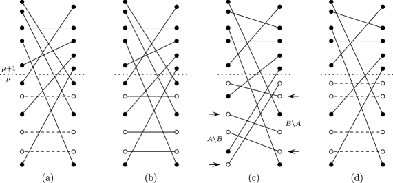
Figure 1: The execution of $\hbox{{rotate\/}}(j_{1},\ldots,j_{k})$, step by step, starting from an example permutation $\pi$. The example is chosen to have $j_{1}>\cdots>j_{k}$. Each of parts (a)–(d) shows $J=\{j_{1},\ldots,j_{k}\}$ on the left and $\pi(J)$ on the right. The sets $\{1,\ldots,\mu\}$ and $\{\mu+1,\ldots,n\}$ are separated by a dotted line. (a): The initial situation. For each $j\in J$, $j$ and $\pi(j)$ are connected by a fully drawn line if $j$ is proper (then $P[j]=\pi(j)$) and by a dashed line if $j$ is improper (then $P[j]$ may be arbitrary). (b): After the execution of $P[j]:=j$ for each improper $j\in J$. Each $j\in J$ is connected to $P[j]$. (c): After the actual rotation. Now $P[j]=\pi^{\prime}(j)$ for all $j\in J$, where $\pi^{\prime}$ is as in Lemma 5.1. The elements of $A\setminus B$ and $B\setminus A$ are indicated by arrows. (d): After the restoration of the invariant. The final permutation is shown with conventions as in part (a).

Let us say that the invariant is violated at some $\ell\in U$ if $\ell\leq\mu$ and $\ell$ is improper in exactly one of $P$ and $P^{-1}$ or $\ell>\mu$ and $\ell$ is improper in at least one of $P$ and $P^{-1}$. Let $J^{\prime}=J\cap\{1,\ldots,\mu\}$, $A=\{j\in J^{\prime}\mid P[j]\leq\mu\}$ and $B=\{P[j]\mid j\in A\}$. Obviously $|A|=|B|$. It can be seen that the invariant is not violated at any element outside of $A\cup B$. Moreover, for $j\in A\cup B$, $j$ is improper in $P$ exactly if $j\in A$, whereas $j$ is improper in $P^{-1}$ exactly if $j\in B$. Therefore the invariant is violated exactly at each $j$ in the symmetric difference of $A$ and $B$. Observe that $|A\setminus B|=|B\setminus A|$ and finally restore the invariant by changing the values of $P$ on $A\setminus B$ to make $P$ map $A\setminus B$ injectively to $\pi^{\prime}(B\setminus A)$ and then setting $P^{-1}[P[j]]:=j$ for all $j\in A\setminus B$. This simultaneously makes the elements of $A\setminus B$ proper in $P$ and makes the elements of $B\setminus A$ improper in $P$ (Fig. 1(d)).

The data structure uses slightly more space than claimed because $\mu$ can take arbitrary values in $\{0,\ldots,n\}$ and so needs $\lceil\log(n+1)\rceil$ bits for its storage. To lower this to $\lceil\log n\rceil$ bits, execute consolidate one first time already as part of the initialization, so that $\mu$ never has the value $n$.

Recall from Section 2 that our main result about systematic choice dictionaries is obtained by the combination of three simple ingredients: A choice dictionary that is wasteful in terms of space (Theorem 5.3), a choice dictionary for very small universes (Lemma 5.5), and the trie-combination method of Section 4.

Theorem 5.3.

There is a choice dictionary that, for arbitrary $n,c\in\mathbb{N}$, can be initialized for universe size $n$ and $c$ colors in constant time and subsequently occupies at most $(2n+4c)\lceil\log(n+1)\rceil+n\lceil\log(2c)\rceil+O(c\log c)=O((n+c)\log(n+c))$ bits and supports color, p-rank, p-select (and hence choice and uniform-choice) and robust iteration in constant time and setcolor in $O(c)$ time. A more precise time bound for setcolor is that the execution of a call $\hbox{{setcolor\/}}(j^{\prime},\ell)$, for all $j^{\prime}\in\{0,\ldots,c-1\}$ and $\ell\in\{1,\ldots,n\}$, takes $O(|j^{\prime}-j|+1)$ time, where $j$ is the color of $\ell$ immediately before the call.

Proof 5.4.

Denote the client vector by $(S_{0},\ldots,S_{c-1})$. The choice dictionary maintains a semipartition $(R_{0},\ldots,R_{2c-1})$ of $U=\{1,\ldots,n\}$, whose sets will be called segments. The intended meaning of the segments is that for $j=0,\ldots,c-1$, $R_{2j}$ and $R_{2j+1}$ are the sets of those elements of $S_{j}$ that are (still) to be enumerated and are not to be enumerated, respectively, in the current iteration over $S_{j}$, if any; thus at all times $R_{2j}\cup R_{2j+1}=S_{j}$. For brevity, let us say that the elements in $R_{k}$ are of hue $k$, for $k=0,\ldots,2c-1$, and denote the hue of each $\ell\in U$ by $\hbox{{hue\/}}(\ell)$. The segments are realized via $2c$ integers $m_{0},\ldots,m_{2c-1}$ that store $|R_{0}|,\ldots,|R_{2c-1}|$, respectively, and a pair $(\pi,\mu)$, where $\pi$ is a permutation of $U$ and $\mu\in\{0,\ldots,n\}$, together with the convention that $\pi$ sorts the elements of $U$ by hue, i.e., $\hbox{{hue\/}}(\pi(1))\leq\cdots\leq\hbox{{hue\/}}(\pi(n))$. We also maintain the prefix sums $s_{k}=\sum_{i=0}^{k}m_{i}$, for $k=-1,\ldots,2c-1$, and the hue of each element of $U\setminus R_{0}$ explicitly in two arrays, so that $\hbox{{hue\/}}(\ell)$ can be determined in constant time for each $\ell\in U$. The invariant $\mu\leq m_{0}$ will hold at all times.

The pair $(\pi,\mu)$ is maintained in an instance $D$ of the data structure of Lemma 5.1. $D$’s rotate operation can be used to move elements from one segment to another. E.g., to move an element $\ell$ from $R_{j}$ to $R_{j^{\prime}}$, where $j<j^{\prime}$, execute $D.\hbox{{rotate\/}}(j_{1},\ldots,j_{k})$, where $(j_{1},\ldots,j_{k})$ is the sequence obtained from $(\pi^{-1}(\ell),s_{j},s_{j+1},\ldots,s_{j^{\prime}-1})$ by eliminating duplicates, i.e., by removing every element equal to an earlier element, and subsequently decrement $m_{j}$ and each of $s_{j},\ldots,s_{j^{\prime}-1}$ and increment $m_{j^{\prime}}$. This takes $O(j^{\prime}-j)$ time. Note how the condition $\mu\leq m_{0}$ prevents unintended transfers of elements from one segment to another by the rotate operation. The operations of the choice dictionary are implemented as follows:

$\hbox{{color\/}}(\ell)$:

Return $\lfloor{{\hbox{{hue\/}}(\ell)}/2}\rfloor$.

$\hbox{{setcolor\/}}_{j}(\ell)$:

If $\hbox{{color\/}}(\ell)\not=j$, then execute $D.\hbox{{consolidate\/}}$ and subsequently move $\ell$ from its current segment to $R_{2j+1}$ and record $\hbox{{hue\/}}(\ell)=2j+1$.

$\hbox{{p-rank\/}}(\ell)$:

Return $\pi^{-1}(\ell)-s_{2j-1}$, where $j=\hbox{{color\/}}(\ell)$.

$\hbox{{p-select\/}}_{j}(k)$:

Return $\pi(s_{2j-1}+k)$ if $1\leq k\leq|S_{j}|=m_{2j}+m_{2j+1}$, and 0 otherwise.

$\hbox{{iterate\/}}_{j}.\hbox{{init\/}}$:

Merge $R_{2j+1}$ into $R_{2j}$, i.e., execute first $m_{2j}:=m_{2j}+m_{2j+1}$ and $s_{2j}:=s_{2j+1}$ and then $m_{2j+1}:=0$.

$\hbox{{iterate\/}}_{j}.\hbox{{more\/}}$:

Return 1 if $R_{2j}\not=\emptyset$, i.e., if $m_{2j}>0$, and 0 otherwise.

$\hbox{{iterate\/}}_{j}.\hbox{{next\/}}$:

Return $0$ if $\hbox{{iterate\/}}.\hbox{{more\/}}=0$. Otherwise execute $D.\hbox{{consolidate\/}}$ and subsequently move the boundary between $S_{2j}$ and $S_{2j+1}$ backward by one element and return the element that crosses the boundary. In other words, decrement $m_{2j}$ and $s_{2j}$, increment $m_{2j+1}$ and return $\pi(s_{2j}+1)$.

The initialization sets $m_{0}:=n$, $m_{j}:=0$ for $j=1,\ldots,2c-1$, $s_{-1}:=0$ and $s_{j}:=n$ for $j=0,\ldots,2c-1$ and initializes $D$. To achieve a constant initialization time, use Lemma 3.1. After the initialization $R_{0}=U$, $R_{1}=\cdots=R_{2c-1}=\emptyset$, $\mu=n$ and $\pi$ is the identity permutation $\hbox{{id\/}}_{n}$, so the client vector represented is $(U,\emptyset,\ldots,\emptyset)$, as required, and the invariant is satisfied. The only operations that may decrease $m_{0}$ are setcolor and $\hbox{{iterate\/}}.\hbox{{next\/}}$, and the decrease is only by 1. Both operations call $D.\hbox{{consolidate\/}}$ before they carry out any other change, so the invariant $\mu\leq m_{0}$ is always satisfied. Only the operation setcolor calls $D.\hbox{{rotate\/}}$, and therefore the elements returned by calls of p-rank and p-select are consistent with bijections that do not change between calls of setcolor. Storing elements that are moved to $S_{j}$ in $R_{2j+1}$ rather than in $R_{2j}$ prevents the elements from being enumerated more than once during an iteration over $S_{j}$. Therefore the iterations over $S_{j}$ are robust.

An accurate count of the size of the data structures introduced above yields an upper bound of $(2n+4c+2)\lceil\log(n+1)\rceil+n\lceil\log(2c)\rceil+O(c\log c)$ bits. To this should be added a number of bits needed to store the parameters $n$ and $c$. On the other hand, we can omit every second prefix sum $s_{i}$, so the space bound stated in the theorem is easily achievable.

Lemma 5.5.

There is a choice dictionary that, for arbitrary $n,c\in\mathbb{N}$, can be initialized for universe size $n$ and $c$ colors in $O(1+{{(n\log c)}/w})$ time and subsequently occupies $n\lceil\log c\rceil$ bits and executes color and setcolor in constant time and successor and predecessor (and hence also choice) in $O(1+{{(n\log c)}/w})$ time.

Proof 5.6.

Store only the $n$ color values, each in a field of $\lceil\log c\rceil$ bits. The realization of $\hbox{{color\/}}(\ell)$ and $\hbox{{setcolor\/}}_{j}(\ell)$ is obvious—read and overwrite the contents of the $\ell$th field, respectively. To execute $\hbox{{successor\/}}_{j}(\ell)$ for $j\in\{0,\ldots,c-1\}$ and $\ell\in\{0,\ldots,n\}$, remove the $\ell$ leftmost fields in a copy, replace the value in every remaining field by its bitwise xor with $j$, and use an algorithm of Lemma 3.3(b). The implementation of predecessor is analogous.

Theorem 5.7.

There is a 2-color systematic choice dictionary that, for arbitrary $n,t\in\mathbb{N}$, can be initialized for universe size $n$ and tradeoff parameter $t$ in constant time and subsequently occupies $n+{n/{(tw)}}+O({n/{(tw)^{2}}}+\log n)$ bits and executes insert, delete, contains, choice, $\overline{\hbox{{choice\/}}}$ and robust iteration over the client set and its complement in $O(t)$ time.

Proof 5.8.

Take $k=tw$ and assume without loss of generality that $k\geq 2$. Compute $q\in\mathbb{N}$ so that $q\geq n^{1/t}$, but $q=O(n^{1/t})$. We compose the choice dictionaries of Theorem 5.3 and Lemma 5.5, both initialized for 2 colors, with the trie-combination method of Section 4 and with the degree sequence $(p_{1},p_{2},\ldots)$, where $p_{1}=p_{2}=k$, $p_{3}=\Theta(\log n)$, and $p_{j}=q$ for $j\geq 4$. Every inner node of height at most 3 in the resulting trie $T$ is equipped with an instance of the choice dictionary of Lemma 5.5, while every node in $T$ of height at least 4 has an instance of the choice dictionary of Theorem 5.3. Every operation on the overall choice dictionary spends $O(t)$ time on each of the three bottom levels of $T$ above the leaves and constant time on every other level. Since the height of $T$ is $O(t)$, this sums to $O(t)$. The choice dictionaries of the nodes in $T$ of height $1$ need a total of exactly $n$ bits, and the most natural layout ensures that the overall dictionary is systematic. The height-2 and height-3 choice dictionaries, if present, need $\lceil n/k\rceil$ bits and $O({n/{k^{2}}})$ bits, respectively. The number of nodes in $T$ of height $4$ is $O(({{{n/{k^{2}}})}/{\log n}})$, so the number of bits required for all instances of the dictionary of Theorem 5.3 is $O({n/{k^{2}}})$.

If we allow the dictionary not to be systematic, we can generalize to several colors and obtain an additional space bound that depends on the maximum size of the client set. In order to support $c$ simultaneous iterations, one for each color, the theorem below requires $O(c\log n)$ additional bits. In general, with enough additional space to keep track of their states, a smaller or larger number of simultaneous iterations can be supported, here and in data structures described later.

Theorem 5.9.

There is a choice dictionary that, for arbitrary $n,c,t,k\in\mathbb{N}$ with $k\log c=O(tw)$, can be initialized for universe size $n$, $c$ colors and tradeoff parameters $t$ and $k$ in constant time and subsequently uses $n\lceil\log_{2}c\rceil+{{cn}/k}+O({{cn}/{k^{2}}}+\log n)$ bits of memory and supports color, setcolor, choice and, given $O(c\log n)$ additional bits, robust iteration in $O(t)$ time. Moreover, as long as the number of elements of nonzero color remains bounded by $m\in\mathbb{N}$, the number of bits of memory used is $O(((t+c)n^{1/t}+ck^{2})m\log n)$. In particular, for every fixed $\epsilon>0$, there is a choice dictionary that executes all operations in constant time and uses $O(cmn^{\epsilon}+1)$ bits to store semipartitions that never have more than $m$ elements of nonzero color.

Proof 5.10.

If $n<8k$, the result follows from Lemma 5.5. Assume therefore that $n\geq 8k$. We use largely the same construction as in the previous proof and with $p_{3}=\Theta(\log n)$ and $q$ chosen as there, but now for general values of $k$ and with $p_{1}=p_{2}=4k$ instead of $p_{1}=p_{2}=k$. There are two additional changes:

First, the choice dictionaries of nodes of height 1 in the trie $T$ are initialized for $c$ rather than 2 colors and, as detailed in Section 4, each choice dictionary of a node of height 2 or more in $T$ is replaced by $c$ independent 2-color choice dictionaries, one for each color. As also discussed in Section 4, this change makes it necessary to keep track explicitly of the initialization of upper and lower trees. Instead of using a single dictionary $D^{*}$ of universe size $\lceil n/{p_{1}}\rceil+c$ as suggested in Section 4, we handle the initialization of the $c$ upper trees in a separate choice dictionary with universe size $c$ (realized according to Theorem 5.7, say) and equip each node $u$ of height 2 with a colorless instance of the choice dictionary of Lemma 5.5 that records the initialization of the choice dictionaries at $u$’s children. The total number of bits needed for the dictionaries that take the place of $D^{*}$ can be bounded by $\lceil n/{p_{1}}\rceil+2c$.

Second, rather than reserving space permanently for every choice dictionary, we allocate space to the $c$ choice dictionaries of a node $u$ of height $\geq 3$ in $T$ only when one of them acquires its first element ($u$ becomes nonempty) and reclaim that space if and when $u$ returns to being empty. When space for the choice dictionaries of a node $u$ of height $\leq 3$ is allocated, we also allocate space for the choice dictionaries of all children of $u$ (and, recursively, for those of their children).

If $n\leq(4k)^{2}$, the height of $T$ is bounded by 2, and its choice dictionaries can be accommodated in a total of $n\lceil\log c\rceil+(c+1)\lceil n/{p_{1}}\rceil+2c\leq n\lceil\log c\rceil+2c({n/{(4k)}}+1)+2c=n\lceil\log c\rceil+c({n/{(2k)}}+4)\leq n\lceil\log c\rceil+{{cn}/k}$ bits, a bound easily seen to be covered by those of the theorem (recall that $k^{2}=\Omega(n)$). In the rest of the proof assume that $n>(4k)^{2}$, so that $T$ is of height at least 3.

The total number of bits needed by the choice dictionaries of the descendants of a node of height 3 is $s_{\mbox{\scriptsize L}}=p_{1}p_{2}p_{3}\lceil\log c\rceil+(c+1)p_{2}p_{3}+cp_{3}$, and these choice dictionaries are accommodated in a leaf chunk of $s_{\mbox{\scriptsize L}}=O(ck^{2}\log n)$ bits. An exception concerns the descendants of the rightmost node of height 3, whose choice dictionaries may need less space; exactly the required number of bits is set aside statically for these dictionaries. In the interest of simplicity, let us ignore this exception for most of the following discussion and return to it briefly at the end of the proof. The $c$ choice dictionaries of a node $u$ of height $\geq 4$ occupy $O(cq\log q)$ bits. Because the neighbors of $u$ in $T$ are no longer stored in fixed places in memory, the representation of $u$ must be augmented by $q+1$ explicit pointers of $O(\log n)$ bits each that allow navigation in $T$. Altogether, $u$ and its choice dictionaries can be accommodated in an inner chunk of $s_{\mbox{\scriptsize I}}=O(q\log n+cq\log q)=O((1+{c/t})q\log n)$ bits.

The total number of nodes of height 3 in $T$ is $n_{\mbox{\scriptsize L}}=\lceil n/{(p_{1}p_{2}p_{3})}\rceil$, and the total number $n_{\mbox{\scriptsize I}}$ of nodes of height $\geq 4$ can be computed in $O(t)$ time. Accordingly, the available memory is conceptually partitioned into $n_{\mbox{\scriptsize L}}$ leaf slots of $s_{\mbox{\scriptsize L}}$ bits each and $n_{\mbox{\scriptsize I}}$ inner slots of $s_{\mbox{\scriptsize I}}$ bits each. When space for a chunk is needed, a free slot of the right size is allocated to it, and returned slots are kept in one of two free lists, one for each chunk size, that can easily be maintained in the free slots themselves. When a free slot is requested, it is taken from the relevant free list unless the latter is empty. If the relevant free list is empty, the first slot of the right size and unused so far is put into service; two simple variables suffice to keep track of the borders between slots that were allocated at least once and new slots.

A leaf slot is exactly as large as the choice dictionaries that may be stored in the slot. An inner slot is larger by the $O(q\log n)$ bits for pointers to other slots, but since the number of inner slots is $O({n/{(qk^{2}\log n)}})$, the total number of additional bits is $O({n/{k^{2}}})$. Therefore the number of bits used by the entire data structure never exceeds $n\lceil\log c\rceil+(c+1)\lceil n/{(4k)}\rceil+O({{cn}/{k^{2}}}+\log n)=n\lceil\log c\rceil+{{cn}/k}+O({{cn}/{k^{2}}}+\log n)$.

As long as the number of elements with nonzero colors remains bounded by $m\in\mathbb{N}$, the data structure allocates at most the first $tm$ inner slots and the first $m$ leaf slots. The total number of bits in these slots is $tms_{\mbox{\scriptsize I}}+ms_{\mbox{\scriptsize L}}=O(tm(1+{c/t})q\log n+cmk^{2}\log n)=O(((t+c)n^{1/t}+ck^{2})m\log n)$. The slots cannot be packed tightly because they are allocated from two different pools, but we can still ensure that they come from a block of memory of $O(((t+c)n^{1/t}+ck^{2})m\log n)$ bits by laying out the slots in memory according to the following pattern: First a leaf slot, then $t$ inner slots, then again a leaf slot, and so on. The space bound easily admits the few choice dictionaries that were allocated statically above.

5.2 A Lower Bound for Systematic Choice Dictionaries

In this subsection we show that the systematic choice dictionary of Theorem 5.7 is optimal, up to a constant factor, in the tradeoff that it offers among redundancy, execution time and word length.

For all integers $h,r,s$, let an $(h,r,s)$-language be a language $L$ over $\Sigma=\{\mathtt{a}_{0},\mathtt{a}_{1},\mathtt{b}_{0},\mathtt{b}_{1}\}$ that does not contain two words of the form $uav_{1}$ and $ubv_{2}$ with $u,v_{1},v_{2}\in\Sigma^{*}$, $a\in\{\mathtt{a}_{0},\mathtt{a}_{1}\}$ and $b\in\{\mathtt{b}_{0},\mathtt{b}_{1}\}$ and for which each $u\in L$ satisfies $|u|=h$, $|u|_{\mathtt{a}_{1}}\leq r$ and $|u|_{\mathtt{b}_{0}}+|u|_{\mathtt{b}_{1}}\leq s$. Here $|u|_{\mathtt{a}_{1}}$, e.g., denotes the number of occurrences of the character $\mathtt{a}_{1}$ in $u$. Let $\mathbb{N}_{0}=\mathbb{N}\cup\{0\}$.

Lemma 5.11.

For all integers $h,r,s$, the cardinality of every $(h,r,s)$-language is bounded by $2^{s^{\prime}}{{h-s^{\prime}+r}\choose r}$, where $s^{\prime}=\min\{h,s\}$.

Proof. For all integers $h,r,s$, let $N(h,r,s)$ be the maximum cardinality of an $(h,r,s)$-language. The bound of the lemma can be shown by induction on $h$ using the recurrence

$$N(h,r,s)=\begin{cases}0,&\mbox{if $h<0$ or $r<0$ or $s<0$};\cr 1,&\mbox{if $h=0$ and $r,s\geq 0$};\cr\hbox{}\,\vbox{\openup 3.0pt\halign{\strut\hfil$\displaystyle{#}$&$\displaystyle{{}#}$\hfil\cr\max\{2&N(h-1,r,s-1),\cr\vglue-1.0pt\cr&N(h-1,r,s)+N(h-1,r-1,s)\}\cr}}\,&\mbox{if $h>0$ and $r,s\geq 0$}.\cr\end{cases} \Box$$

Theorem 5.12.

Let $n,s,t\in\mathbb{N}_{0}$, let $n\geq 2$ and assume that some systematic data structure $D$ can represent every subset of $U=\{1,\ldots,n\}$ in a sequence $B$ of $n+s$ bits. Assume further that for each $r\in\{1,\ldots,n\}$, it is possible to distinguish among the $n\choose r$ subsets $S$ of $U$ of size $r$ with at most $rt$ bit probes to an arbitrary sequence $B(S)$ that represents each set $S$ according to $D$’s conventions. Then $(s+{1/{\ln 2}})t\geq{n/{(e\ln 2)}}$ and, if $s>0$, $st\geq{n/2}$.

Proof 5.13.

The second assumption of the theorem cannot hold for $t=0$. We can therefore assume without loss of generality that $t\geq 1$ and that $s\leq n$. For an $r\in\{1,\ldots,n\}$ to be chosen later, we associate a word $u_{S}$ over $\Sigma$ with each $S\in\mathcal{S}=\{S\subseteq\{1,\ldots,n\}:|S|=r\}$. Let $\mathcal{A}$ be an algorithm that can distinguish among the sets in $\mathcal{S}$ with at most $rt$ bit probes. Without loss of generality, $\mathcal{A}$ probes no bit more than once. For each $S\in\mathcal{S}$, we apply $\mathcal{A}$ to a bit sequence $B(S)$ used by $D$ to represent $S$ and chosen to be minimal in the sense that no sequence $B\not=B(S)$ of $n+s$ bits that also represents $S$ satisfies $B\leq B(S)$, where $\leq$ denotes the conjunction of bitwise $\leq$ in all bit positions. Informally, the minimality of $B(S)$ implies that every uninitialized bit in $B(S)$ has the value 0. Without loss of generality, assume that the first $n$ bits of $B(S)$ are the bits $b_{1},\ldots,b_{n}$ referred to in the definition of a systematic data structure (informally, the bit-vector representation of $S$). For each $S\in\mathcal{S}$, $u_{S}$ is obtained as follows: Initialize $u_{S}$ to be the empty word and append a character to $u_{S}$ at each probe carried out by $\mathcal{A}$ on input $B(S)$, choosing the character as $c_{i}$, where $i\in\{0,1\}$ is the value of the bit probed, $c=\mathtt{a}$ if the bit probed is among the first $n$ bits of $B(S)$, and $c=\mathtt{b}$ if the bit probed is among the last $s$ bits of $B(S)$. At this point, since $\mathcal{A}$ uses at most $h=rt$ probes, $|u_{S}|\leq h$. Finally increase $|u_{S}|$ to exactly $h$ by appending $h-|u_{S}|$ occurrences of $\mathtt{a}_{0}$ to $u_{S}$.

For each $S\in\mathcal{S}$, with $u=u_{S}$, $\mathcal{A}$ probes each bit at most once, and so $|u|_{\mathtt{a}_{1}}\leq r$ since $B(S)$ is minimal and $|S|=r$, and $|u|_{\mathtt{b}_{0}}+|u|_{\mathtt{b}_{1}}\leq s$ since there are only $s$ bits in addition to $b_{1},\ldots,b_{n}$. $L=\{u_{S}\mid S\in\mathcal{S}\}$ is therefore an $(h,r,s)$-language. For $S_{1},S_{2}\in\mathcal{S}$ with $S_{1}\not=S_{2}$, we cannot have $u_{S_{1}}=u_{S_{2}}$, so Lemma 5.11 shows that

$${n\choose r}=|\mathcal{S}|=|L|\leq 2^{s^{\prime}}{{h-s^{\prime}+r}\choose r},$$

where $s^{\prime}=\min\{h,s\}$. If $s=0$, choose $r=1$, which turns the inequality $(*)$ into $n\leq t+1$ or $t\geq n-1$. Adding $t\geq 1$, we obtain $t\geq{n/2}$, which implies the inequality $(s\ln 2+1)t\geq{n/e}$ of the theorem. In the following assume that $s\geq 1$.

We will make sure to choose $r\leq s$ and therefore $r\leq s^{\prime}$, so that $h-s^{\prime}+r\leq h$. Then, since $h=rt\leq st$, we may assume without loss of generality that $h\leq n$. Now

$$2^{s}\geq 2^{s^{\prime}}\geq{{n\choose r}\Biggm{/}{h\choose r}}={{n(n-1)\cdots(n-r+1)}\over{h(h-1)\cdots(h-r+1)}}\geq\left({n\over h}\right)^{r}=\left({n\over{rt}}\right)^{r}.$$

If we choose $r=s$, the requirement $r\leq s$ is certainly satisfied, $(**)$ becomes

$$2^{s}\geq\left({n\over{st}}\right)^{s},$$

and the inequalities $2\geq{n/{(st)}}$ and $st\geq{n/2}$ follow. If $t\leq{n/e}$ and we instead choose $r=\lfloor{n/{(et)}}\rfloor\geq 1$, the inequality $s\geq{n/{(2t)}}$ that was just established shows that the requirement $r\leq s$ is again satisfied. With this choice of $r$, ${n/{(rt)}}\geq e$ and therefore $2^{s}\geq e^{r}$ and $s\ln 2+1\geq r+1\geq{n/{(et)}}$. Thus $(s\ln 2+1)t\geq{n/e}$, a relation that also holds if $t>{n/e}$. The theorem follows.

Corollary 5.14.

Let $n\in\mathbb{N}$ and $s\in\mathbb{N}_{0}$ and let $D$ be a systematic choice dictionary with universe size $n$ that never occupies more than $n+s$ bits. Let $t_{\mathit{delete}}$ and $t_{\mathit{choice}}$ be upper bounds on the number of bits read from memory during an execution of $D$’s operations delete and choice, respectively (the two quantities may depend on $n$). Then $(s+{1/{\ln 2}})(t_{\mathit{delete}}+t_{\mathit{choice}})\geq{n/{(e\ln 2)}}$ and, if $s>0$, $s(t_{\mathit{delete}}+t_{\mathit{choice}})\geq{n/2}$.

Proof 5.15.

The return value of choice cannot be independent of $D$’s client set $S$, so we must have $t_{\mathit{choice}}\geq 1$. We can therefore assume without loss of generality that $n\geq 2$.

Given knowledge of $r=|S|$, we can output $S$ with $r$ iterations of a loop in which an element of $S$ is first obtained with a call of choice and subsequently output and removed from $S$ with a call of delete. The procedure reads at most $r(t_{\mathit{delete}}+t_{\mathit{choice}})$ bits of $D$’s representation of $S$, i.e., Theorem 5.12 can be applied with $t=t_{\mathit{delete}}+t_{\mathit{choice}}$.

With a very similar argument we can obtain a lower bound on the amortized complexity of insert, delete and choice.

Corollary 5.16.

Let $n\in\mathbb{N}$ and $s\in\mathbb{N}_{0}$ and let $D$ be a systematic choice dictionary with universe size $n$ that never occupies more than $n+s$ bits. Fix an arbitrary potential function for $D$ and assume that every representation of the empty client set has the same potential. Let $t_{\mathit{insert}}$, $t_{\mathit{delete}}$ and $t_{\mathit{choice}}$ be upper bounds on the worst-case amortized number of bits read from memory during $D$’s execution of insert, delete and choice, respectively (the three quantities may depend on $n$). Then $(s+{1/{\ln 2}})(t_{\mathit{insert}}+t_{\mathit{delete}}+t_{\mathit{choice}})\geq{n/{(e\ln 2)}}$ and, if $s>0$, $s(t_{\mathit{insert}}+t_{\mathit{delete}}+t_{\mathit{choice}})\geq{n/2}$.

Proof 5.17.

As above, assume without loss of generality that $n\geq 2$. For every $r\in\{1,\ldots,n\}$ and every $S\subseteq\{1,\ldots,n\}$ with $|S|=r$, we can take $D$ from its initial state with empty client set via a state in which its client set is $S$ and back to a state with empty client set using exactly $r$ calls of each of insert, delete and choice. By assumption, the final potential is the same as the initial potential, so the total amortized number of bits read is the same as the total actual number of bits read. Therefore Theorem 5.12 is applicable with $t=t_{\mathit{insert}}+t_{\mathit{delete}}+t_{\mathit{choice}}$.

With $n$, $s$ and $t$ as in Theorem 5.12, the theorem states that $(s+O(1))t\geq\alpha n$, where $\alpha={1/{(e\ln 2)}}\approx 0.53$. We complement this result by showing that for every sufficiently easily computable function $t:\mathbb{N}\to\mathbb{N}$ with $t(n)=\omega(\log n)$ but $t(n)=o(n)$, there is a 2-color systematic choice dictionary $D$ that, when initialized for universe size $n\in\mathbb{N}$, reads $t(n)+o(t(n))$ bits of its internal representation during the execution of each operation and has a redundancy $s(n)$ for which $s(n)t(n)=n+o(n)$. $D$ is simple. It is a three-level trie constructed as described in Section 4 with the degree sequence $(p_{1},p_{2},p_{3})$, where $p_{1}=t(n)$, $p_{2}=\Theta(\sqrt{t(n)\log n})$ and $p_{3}=n$. The two bottom levels of choice dictionaries are realized according to Lemma 5.5 with $c=2$, whereas the choice dictionary of the root is an instance of that of Theorem 5.3, again with $c=2$. The redundancy of the overall choice dictionary is $\lceil{n/{p_{1}}}\rceil+O(1+({n/{(p_{1}p_{2})}})\log n)=({n/{t(n)}})(1+o(1))$, and it is easy to see that the number of bits read during the execution of an operation is bounded by $p_{1}+p_{2}+O(\log n)=t(n)(1+o(1))$. The product of the two, indeed, is $n+o(n)$.

6 Restricted and Extended Choice Dictionaries

6.1 A Data Structure with insert and extract-choice

The main result of this subsection (Theorem 6.4) is a choice-like dictionary with universe size $n$ that stores a client set $S$ of size $m$ in fewer than $n$ bits even when $m$ is not much smaller than $n$. More precisely, the number of bits used is $O(m\log(2+{n/{(m+1)}})+1)$. Since $\log{n\choose m}\geq\log(({n/m})^{m})=m\log({n/m})$ for $m>0$, the space used by our data structure is within a constant factor of the information-theoretic lower bound for most combinations of $n$ and $m$. What we show is that this tight space bound still admits certain dynamic operations. More precisely, we can support insertion and the operation extract-choice that returns and deletes an (arbitrary) element of $S$, but neither unrestricted deletion nor queries about specific elements such as contains.

There is an apparent conflict between fast insertion and a very space-efficient representation in fewer than $n$ bits. To represent the client set $S$ using little space, we can store it in difference form, i.e., as the sequence of differences between successive elements of $S$ (in sorted order). With this representation, however, insertion is easily seen to be prohibitively expensive. On the other hand, insertion is easy if we store the elements of $S$ in no particular order, but then we need about $\log n$ bits per element of $S$, which is excessive. Our solution is to store $S$ permanently in difference form, but to insert new elements into an unsorted buffer. The buffer is wasteful of space, and so has to be sorted and merged into the rest of $S$ before it becomes too large. Because every operation is supposed to work in constant time, this entails a certain technical complexity. As a warm-up before tackling this, we illustrate the use of the difference form by developing a data structure of possible independent interest, a space-efficient stack that requires its elements to occur in sorted order at all times.

Definition 6.1.

A bounded-universe sorted stack is a data structure that, for every $n\in\mathbb{N}$, can be initialized for universe size $n$ and subsequently maintains an initially empty sequence $(x_{1},\ldots,x_{m})$ with $1\leq x_{1}\leq\cdots\leq x_{m}\leq n$ while supporting the following operations:

$\hbox{{sorted-push\/}}(x)$

($x\in\{1,\ldots,n\}$): Replaces $(x_{1},\ldots,x_{m})$ by $(x_{1},\ldots,x_{m},x)$ if $x_{m}\leq x$ and does nothing otherwise.

pop:

Replaces $(x_{1},\ldots,x_{m})$ by $(x_{1},\ldots,x_{m-1})$ and returns $x_{m}$ if $m>0$; returns 0 and does nothing else if $m=0$.

Lemma 6.2.

There is a bounded-universe sorted stack that, for arbitrary $n\in\mathbb{N}$, can be initialized for universe size $n$ in constant time, subsequently supports sorted-push and pop in constant time and, when it currently holds a sequence $(x_{1},\ldots,x_{m})$ of $m\in\mathbb{N}_{0}$ elements, uses at most $m\log(q+1)+O(m\log\log(q+4)+\log n+1)$ bits, where $q={{(n-1)}/{(m+1)}}$.

Proof 6.3.

We encode integers using a scheme quite similar to Elias’ $\delta$ representation [19]: Every nonnegative integer $d$ can be represented in binary in $\lfloor\lambda(d)\rfloor$ bits, where $\lambda(d)=\log(d+1)+1$ for all $d\in\mathbb{N}_{0}$, but this presupposes knowledge of the length of the representation of $d$, i.e., of $\lfloor\lambda(d)\rfloor$. To add this information, we append to the representation of $d$ a sequence of $\ell=\lfloor\lambda(\lfloor\lambda(d)\rfloor)\rfloor$ bits that encode $\lfloor\lambda(d)\rfloor$, followed by another $\ell+1$ bits that encode $\ell$ suitably in unary. Altogether, this encodes $d$ in a string of at most $\lambda(d)+3\lambda(\lambda(d))$ bits that, read backwards, can be decoded in constant time without prior knowledge of the length of the string.

With $x_{0}=1$ and $x_{m+1}=n$, we store a bit string $B$ that encodes $(d_{1},\ldots,d_{m+1})$, where $d_{i}=x_{i}-x_{i-1}$, for $i=1,\ldots,m+1$, is encoded as described above and the encodings of $d_{1},\ldots,d_{m+1}$ are simply concatenated. Before storing $B$ itself, we store the encoding of its length $|B|$, so that we can find the end of $B$ in constant time. By the implicit assumption $n,m<2^{w}$, $O(w)$ bits suffice for this purpose. Accordingly, we always store $|B|$ in a field of $\kappa w$ bits for some suitable constant $\kappa\in\mathbb{N}$. In order not to waste the last part of the field, however, we move to there a suffix of $B$ of the appropriate length.

It is easy to see that the operations sorted-push and pop can be supported in constant time. $|B|$ is bounded by $\sum_{i=1}^{m+1}(\lambda(d_{i})+3\lambda(\lambda(d_{i})))$. Because $\sum_{i=1}^{m+1}d_{i}=n-1$ and $\lambda$ and $\lambda\circ\lambda$ are concave on the set of nonnegative real numbers, $|B|\leq(m+1)(\lambda(q)+3\lambda(\lambda(q)))$ by Jensen’s inequality. Since the number of bits used is $|B|+O(\log|B|)$, the lemma follows.

Theorem 6.4.

There is a data structure $D$ with the following properties: First, for every $n\in\mathbb{N}$, $D$ can be initialized for universe size $n$ in constant time and subsequently maintains an initially empty multiset $S$ with elements drawn from $U=\{1,\ldots,n\}$ and executes the following operations in constant time:

$\hbox{{insert\/}}(\ell)$

($\ell\in U$): Inserts (another copy of) $\ell$ in $S$.

extract-choice:

Removes an arbitrary (copy of an) element of $S$ and returns it.

Second, $D$ allows robust iteration over $S$ in constant time per element enumerated, and when the current size of $S$ (counting each element with its multiplicity) is $m\in\mathbb{N}_{0}$, the number of bits used by $D$ is $O(m\log(2+{n/{(m+1)}})+1)$.

Proof 6.5.

A single bit indicates whether $S=\emptyset$. If this is not the case, $S$ is realized as the disjoint union of four multisets, $S_{1}$, $S_{2}$, $S^{*}_{1}$ and $S^{*}_{2}$. $S_{1}$ and $S_{2}$ are called reservoirs. The elements of each reservoir are stored in sorted order in a data structure that is exactly as the bounded-universe sorted stack of Lemma 6.2, except that the binary representation of each difference between consecutive elements is not only followed, but also preceded by an encoding of its length. Thus a reservoir can be read both in the forward and in the backward direction, and it respects the space bound even if it contains all $m$ elements of $S$. $S^{*}_{1}$ and $S^{*}_{2}$ are called buffers. For $i=1,2$, the elements of $S^{*}_{i}$ are stored in no particular order in an array of $|S^{*}_{i}|$ cells of $\lceil\log n\rceil$ bits each. We also store $|S^{*}_{1}|$ and $|S^{*}_{2}|$, and the representations of $S_{1}$, $S_{2}$, $S^{*}_{1}$, $S^{*}_{2}$, $|S^{*}_{1}|$ and $|S^{*}_{2}|$ are interleaved in memory so that the space occupied by them is within a constant factor of the size of a largest among them.

At all times, exactly one buffer is called active. New elements are always inserted in the active buffer. Consider a particular point in time and let $k\in\{1,2\}$ be the index of the active buffer at that time. As soon as $S^{*}_{k}$ both contains at least $2\sqrt{n}$ elements and occupies at least as many bits as $S_{k}$, it stops being active, and the other buffer, $S^{*}_{3-k}$, which is empty at this time, takes over as the active buffer. From this point on, in a background process carried out piecemeal and interleaved with the execution of calls of insert and extract-choice, $S^{*}_{k}$ is sorted in linear time with 2-phase radix sort and merged with $S_{k}$. The resulting sequence is stored in $S_{3-k}$, after which $S^{*}_{k}$ and $S_{k}$ are emptied. While $S_{3-k}$ is under construction, its size is artificially taken to be $\infty$, in the sense that $S^{*}_{3-k}$ is kept active at least until $S_{3-k}$ is finished. The elements to be removed and returned by calls of extract-choice are taken from $S_{k}$ during the sorting of $S^{*}_{k}$ and from $S_{3-k}$ during the merge of $S^{*}_{k}$ and $S_{k}$. The background process should be fast enough to keep $S_{k}$ nonempty during the sorting of $S^{*}_{k}$, to keep $S_{3-k}$ nonempty once the merge has started, and to complete before $S^{*}_{3-k}$ occupies as many bits as $S_{3-k}$ will when it is finished.

In order for the background process to require only constant time per operation executed by $D$, the merge of $S_{k}^{*}$ with $S_{k}$ to obtain $S_{3-k}$ must happen in $O(|S_{k}^{*}|)$ time, which generally means sublinear time with respect to the number of elements in the reservoir $S_{k}$. Using the compactness of the representation of $S_{k}$, we achieve this by carrying out the merge using table lookup. Recall that $S_{k}$ and $S_{3-k}$ are stored in difference form. During the merge, we therefore keep track of the element most recently removed from $S_{k}$ and the element most recently written to $S_{3-k}$, so that future elements can be decoded or encoded correctly. As detailed above, the elements of $S_{k}$ are represented through variable-length bit segments, each complete with its length encoding. At any given time during the merge, initial parts of $S_{k}^{*}$ and $S_{k}$ have been merged, while the remaining elements are still to be processed. To continue the merge, we use table lookup to find the last element, $x$, of $S_{k}$, if any, whose segment is fully contained in the next $\lfloor({1/5)}\log n\rfloor$ bits of the representation of $S_{k}$. If $x$ exists and is no larger than the next element $x^{*}$ of $S_{k}^{*}$ ($\infty$ if $S_{k}^{*}$ is exhausted), the elements of $S_{k}$ up to and including $x$ can be moved from $S_{k}$ to the output sequence $S_{3-k}$. If $x$ exists but $x^{*}<x$, all remaining elements of $S_{k}$ no larger than $x^{*}$ can be identified with a second table lookup (applied to the next $\lfloor({1/5})\log n\rfloor$ bits of the representation of $S_{k}$ and the difference between the first elements of $S_{k}$ and $S_{k}^{*}$, a total of at most $({2/5})\log n$ bits) and moved to $S_{3-k}$. In both cases, subsequently the first remaining element of $S_{k}$ ($\infty$ is $S_{k}$ is exhausted) can be compared with $x^{*}$, and the smaller of the two can be moved to $S_{3-k}$. All of this takes constant time, and it consumes $\Omega(\log n)$ bits of the representation of either $S_{k}$ or $S_{k}^{*}$. Therefore the total time needed to sort $S^{*}_{k}$ and to merge it with $S_{k}$ is $O(|S^{*}_{k}|)$. As anticipated above, this shows that executing a constant number of steps of the background process for each call of insert and extract-choice suffices to let the process finish in time. Thus $D$ executes every operation in constant time.

The tables needed for the merge occupy $O(\sqrt{n})$ bits and can be constructed in $O(\sqrt{n})$ time. This happens in another background process that is advanced by a constant number of steps (if it has not completed) whenever the active buffer contains at least $\sqrt{n}$ elements and that finishes before the active buffer reaches $2\sqrt{n}$ elements. Whenever the number of elements in the active buffer drops below $\sqrt{n}$—in particular, when an empty buffer becomes active—the tables are discarded, so that the space that they occupy is always within a constant factor of that taken up by the active buffer.

In order to support robust iteration over $S$, we add more structural information to the data structure. Call an element of $S$ live if it was present in $S$ at the time of the most recent preceding call of $\hbox{{iterate\/}}.\hbox{{init\/}}$, if any, and has not since been enumerated. If an element of $S$ is not live, it is dead. An initial part of each reservoir or buffer that was not emptied since the most recent preceding call of $\hbox{{iterate\/}}.\hbox{{init\/}}$ (informally, that existed at that time) is marked off as its live area. If one or more live areas are nonempty just before a call of $\hbox{{iterate\/}}.\hbox{{next\/}}$, the next element enumerated is the last element of some live area. If the last element of a live area is enumerated or deleted in a call of extract-choice, the live area shrinks by one element. A call of $\hbox{{iterate\/}}.\hbox{{init\/}}$ sets the live area of each reservoir and of each buffer to be the entire reservoir or buffer. This is the only occasion on which a live area expands.

When a buffer is sorted and merged with a reservoir to create a new reservoir, the live elements can no longer be kept in a contiguous area. On the other hand, constant-time iteration is possible only if the next live element to be enumerated can be found in constant time. For this reason reservoirs and buffers created since the most recent preceding call of $\hbox{{iterate\/}}.\hbox{{init\/}}$ have empty live areas, and the live elements in each such reservoir are kept in a linked list in the opposite of the order in which they occur in the reservoir. Each live element in the list is labeled by its distance, measured in bits, to the next live element in the list. It is easy to see that the labels do not add to the total space requirements by more than a constant factor (small labels could even be represented in unary). Any list labels present in the live area of a reservoir are ignored—all elements in the live area are alive.

Before a buffer is sorted in preparation for being merged with a reservoir, each buffer element is given a bit of satellite data that indicates whether the element is alive or dead. The bit is carried along with the element during the sorting and used in the merge to equip the resulting reservoir with the linked list of its live elements described above. The table that drives the merge, instead of merely indicating a number of bits that can be copied from the old to the new reservoir, must be changed to supply a “piece of reservoir” complete with list labels. The at most one label that points outside of the current piece, namely to an element in the part of the new reservoir that has already been constructed (the nonlocal pointer), must be filled in separately and outside of the table lookup. Correspondingly, it is convenient to split the table lookup into two: The first table lookup yields the piece of reservoir that precedes the nonlocal pointer (thus the piece specifies only dead elements), and the second table lookup yields the piece of reservoir that follows it (if there is no nonlocal pointer, let the first table lookup provide the entire piece of reservoir). Even with these additional computational steps, the time and space bounds established above remain valid.

Since an iteration enumerates only elements that were present when the iteration started and were not deleted before their enumeration, iterations are robust.

As is easy to see, the data structure of Theorem 6.4 also supports constant-time choice. This operation, however, is not likely to be very useful except in the combination extract-choice.

6.2 A Data Structure with color and setcolor

In this subsection we reconsider a data structure of Dodis et al. [18] and extend it to support constant-time initialization. The data structure basically emulates $c$-ary memory, for arbitrary $c\geq 2$, on standard binary memory almost without losing space. This is essential to the choice dictionaries of Subsection 6.3 and Section 7 in the case where the number of colors is not a power of 2.

For $b=\lfloor\log n\rfloor$ the following lemma essentially coincides with the result of Dodis et al. Only in extreme cases can it be useful to choose smaller values for $b$, but we need the present form of Lemma 6.6 to prove Lemma 7.15 in full generality. In Lemma 6.6 and Theorem 6.8 the sequence $(c_{1},\ldots,c_{n})$ is assumed to be represented in a way that allows it to be communicated to the initialization routine in constant time, most naturally as a list of constant length of (value, multiplicity) pairs.

Lemma 6.6.

There is a data structure that, for all given $n,b\in\mathbb{N}$ and for every given sequence $(c_{1},\ldots,c_{n})$ of $n$ positive integers with $|\{\ell\in\mathbb{N}:1\leq\ell<n$ and $c_{\ell}\not=c_{\ell+1}\}|=O(1)$, can be initialized in constant time and subsequently occupies $\sum_{\ell=1}^{n}\log c_{\ell}+O({n/{2^{b}}}+\log n+1)$ bits, needs access to a table of $O(b^{2})$ bits that can be computed in $O(b)$ time and depends only on $n$, $b$ and $(c_{1},\ldots,c_{n})$, and maintains a sequence $(a_{1},\ldots,a_{n})$ drawn from $\{0,\ldots,c_{1}-1\}\times\cdots\times\{0,\ldots,c_{n}-1\}$ under constant-time reading and writing of individual elements in the sequence. The data structure does not initialize the sequence.

Proof 6.7.

Dodis et al. [18] considered the fundamental problem of realizing an array of $n$ entries, each drawn from a set of the form $\{0,\ldots,c-1\}$ for integer $c\geq 2$. They described a beautifully simple construction that allows individual array entries (called small digits in what follows) to be read and written in constant time, yet needs just $n\log c+O(1)$ bits (the authors even argue that $\lceil n\log c\rceil$ bits suffice). A few details not considered by Dodis et al. can easily be handled: (1) The authors actually group $r$ small digits into one big digit drawn from $\{0,\ldots,c^{r}-1\}$, where $r\in\mathbb{N}$ is chosen to make $c^{r}=\Theta(n^{2})$, and accordingly store approximately $n/r$ big digits instead of $n$ small digits. The proof in fact is correct for arbitrary $r$ as long as $c^{r}$ is $\Omega(n^{2})$ (but still $2^{O(w)}$, so that big digits can be manipulated in constant time); this allows us to handle values of $c$ larger than $\Theta(n^{2})$. (2) The big digits are associated with the nodes of a binary tree $T$. The proof remains correct if the big digit associated with the root of $T$ in fact is drawn from a smaller domain than the other big digits; this allows us to deal with the fact that $r$ may not divide $n$. (3) The construction needs a table $Y$ of $O((\log n)^{2})$ bits of precomputed numbers that depend on $n$ and $c$. The authors do not mention the time needed to obtain $Y$ from $n$ and $c$, but it is easy to see that it can be done in $O(\log n)$ time, namely constant time per level in $T$. In particular, a part of $Y$ indicates the size and memory layout of the data structure. The same time allows us to compute the powers $c^{i}$, for $i=2,\ldots,r$, which are needed to extract small digits from big digits and update small digits within big digits in constant time.

Lemma 6.6 follows by splitting the sequence $(a_{1},\ldots,a_{n})$ into $O(1+{n/{2^{b}}})$ subsequences $(a_{i},\ldots,a_{j})$ with $c_{i}=\cdots=c_{j}$ and $j-i=O(2^{b})$ and applying the construction of Dodis et al. independently to each such subsequence.

For $n\in\mathbb{N}$ and $\epsilon>0$, let us call a sequence $(c_{1},\ldots,c_{n})$ of $n$ positive integers $\epsilon$-balanced if $\epsilon(\log n)^{2}\sum_{\ell\in S}\log c_{\ell}\leq\sum_{\ell=1}^{n}\log c_{\ell}$ for all $S\subseteq\{1,\ldots,n\}$ with $|S|\leq(\log n)^{3}$. The theorem below requires $(c_{1},\ldots,c_{n})$ to be $\epsilon$-balanced for some fixed $\epsilon>0$. While this requirement is necessary for our proof, it is a technicality of scant interest. In order for a sequence $(c_{1},\ldots,c_{n})$ not to be $\epsilon$-balanced for any fixed $\epsilon>0$, at least some of its elements must be very large relative to $n$. Indeed, provided that $c_{i}\geq 2$ for $i=1,\ldots,n$, our implicit convention $\log c_{i}=O(w)$ for $i=1,\ldots,n$ implies that the condition of $\epsilon$-balance is automatically satisfied for some fixed $\epsilon>0$ if $w=O({n/{(\log n)^{5}}})$.

Theorem 6.8.

For all fixed $\epsilon>0$, there is a data structure that, for all given $n\in\mathbb{N}$ and for every given $\epsilon$-balanced sequence $(c_{1},\ldots,c_{n})$ of $n$ integers with $c_{\ell}\geq 2$ for $\ell=1,\ldots,n$ and $|\{\ell\in\mathbb{N}:1\leq\ell<n$ and $c_{\ell}\not=c_{\ell+1}\}|=O(1)$, can be initialized in constant time and subsequently occupies $\sum_{\ell=1}^{n}\log_{2}c_{\ell}+O((\log n)^{2}+1)$ bits and maintains a sequence $(a_{1},\ldots,a_{n})$ of $n$ integers, drawn from $\{0,\ldots,c_{1}-1\}\times\cdots\times\{0,\ldots,c_{n}-1\}$, under constant-time reading and writing of individual elements in the sequence. The data structure does not initialize the sequence. For $\ell=1,\ldots,n$, the parameter $c_{\ell}$ may be presented to the data structure in the form of a pair $(x_{\ell},y_{\ell})$ of positive integers with $c_{\ell}=x_{\ell}^{y_{\ell}}$ and $y_{\ell}=n^{O(1)}$.

Proof 6.9.

Let $Y$ be the table used by the data structure of Lemma 6.6. Aside from the question of $(c_{1},\ldots,c_{n})$ being $\epsilon$-balanced, the only essential difference between Theorem 6.8 and Lemma 6.6 is that the theorem does not assume $Y$ to be externally available. The theorem provides space for storing $Y$, but no time for computing it before the first operation must be served. Assume without loss of generality that $n\geq 2$ and let $U=\{1,\ldots,n\}$ and $b=\lfloor\log n\rfloor$. Recall that $Y$ can be computed from $(c_{1},\ldots,c_{n})$ in $O(b)$ time—if necessary, this time bound also allows for the calculation of $c_{\ell}$ from $x_{\ell}$ and $y_{\ell}$ for $\ell=1,\ldots,n$ via repeated squaring.

Consider first the special case $c_{1}=\cdots=c_{n}=c$. We allocate first $\Theta(b^{2})$ bits for $Y$, then a block of $\Theta(b\log b)$ additional bits whose use will be explained later, and finally space for a data structure $D^{\mbox{\scriptsize T}}$. $D^{\mbox{\scriptsize T}}$ is a trie of constant depth with $n$ potential leaves, the $\ell$th of which, for $\ell=1,\ldots,n$, holds $a_{\ell}$ in $\lceil\log c\rceil$ bits if $a_{\ell}$ has changed from its initial value of 0. Disregarding the question of space, $D^{\mbox{\scriptsize T}}$ can provide the functionality promised in the theorem. Choose the (constant) depth of $D^{\mbox{\scriptsize T}}$ to be at least $4$. We will use $D^{\mbox{\scriptsize T}}$ for at most $2b$ operations. Thus, even without paying particular attention to economy of space, we can easily ensure that the number of bits needed for $D^{\mbox{\scriptsize T}}$ is $O(2b(n^{{1/4}}\log n+\log c))$ and therefore, for $n$ larger than a constant, at most $({1/{(2b+2)}})n\log c$.

We construct $Y$ in a background process interleaved with the execution of the first $b$ operations (the first phase), using $D^{\mbox{\scriptsize T}}$ to serve these $b$ operations. At the end of the first phase, when $Y$ is ready, we start running an instance $D$ of the data structure of Lemma 6.6 in parallel with $D^{\mbox{\scriptsize T}}$, making sure that every $\ell\in U$ that is written to after the first phase has the correct associated value in $D$ and, if $\ell$ is still present in $D^{\mbox{\scriptsize T}}$, in $D^{\mbox{\scriptsize T}}$. Interleaved with the execution of the second group of $b$ operations (the second phase), we empty $D^{\mbox{\scriptsize T}}$ element by element, making sure that every element deleted from $D^{\mbox{\scriptsize T}}$ has the correct value in $D$—informally, we transfer the element from $D^{\mbox{\scriptsize T}}$ to $D$. To determine $a_{\ell}$ for some $\ell\in\{1,\ldots,n\}$ in the second phase, we first query $D^{\mbox{\scriptsize T}}$. If $\ell$ is present in $D^{\mbox{\scriptsize T}}$, the associated value is returned. Otherwise we return the value associated with $\ell$ in $D$. All operations can still be executed in constant time during the parallel operation of $D$ and $D^{\mbox{\scriptsize T}}$. After the second phase, $D^{\mbox{\scriptsize T}}$ is empty and can be considered to have disappeared.

A problem that was ignored until now is that $D^{\mbox{\scriptsize T}}$ and $D$ must use the same memory area during the second phase. Partition $U$ into $2b+2$ sectors $U_{1},\ldots,U_{2b+2}$ of consecutive elements, all of the same size $n^{\prime}$, except that $U_{2b+2}$ may be smaller. We call $U_{1}$ the forbidden sector and $U_{2b+2}$ the incomplete sector. $D$ is in fact split into three instances of the data structure of Lemma 6.6: $D_{1}$, whose universe is the forbidden sector $U_{1}$, and two instances $D_{*}$ and $D_{2b+2}$ whose universes are $\bigcup_{i=2}^{2b+1}U_{i}$ and $U_{2b+2}$ (both translated suitably to begin at 1), respectively. At the end of the first phase, aided by $Y$, we can compute the exact number of bits required for each of $D_{1}$, $D_{*}$ and $D_{2b+2}$ in constant time. Overlapping the memory space used for $D^{\mbox{\scriptsize T}}$, we allocate space first for $D_{1}$ and then for $D_{*}$ and $D_{2b+2}$. Since $D_{1}$ occupies at least $n^{\prime}\log c$ bits and $D^{\mbox{\scriptsize T}}$ occupies at most $n^{\prime}\log c$ bits, $D_{1}$ is the only component of $D$ whose memory area overlaps that of $D^{\mbox{\scriptsize T}}$.

During the transfer of elements from $D^{\mbox{\scriptsize T}}$ to $D$ in the second phase, it is easy to handle elements outside of the forbidden sector. As concerns elements destined for $D_{1}$, however, a problem arises because $D_{1}$ overlaps $D^{\mbox{\scriptsize T}}$, which is still in use. In order to circumvent this problem, we will ensure that during the execution of the first $2b$ operations, no element located in the forbidden sector acquires a nonzero value. We achieve this by storing the elements not directly, but according to a rudimentary hash function that is data-dependent and defined in a lazy manner. The hash function takes the form of a bijection $g$ from $U$ to itself. Every element in the incomplete sector is mapped to itself by $g$, and the rest of $g$ is induced by a permutation $\pi$ of $I=\{1,\ldots,2b+1\}$ in the following way: For each $i\in I$, the $\ell$th element of $U_{i}$ is mapped by $g$ to the $\ell$th element of $U_{\pi(i)}$, for $\ell=1,\ldots,n^{\prime}$. Arguments in $U$ of operations to be executed are mapped under $g$ before being passed on to one of the three components of $D$, and answers obtained from the components of $D$ are mapped under $g^{-1}$ to obtain the appropriate return values. The permutation $\pi$ and its inverse must be stored in the data structure, the necessary space being furnished by the block of $\Theta(b\log b)$ bits allocated but not used so far.

It remains to describe the permutation $\pi$ of $I$. When an element outside of the incomplete sector is first given a nonzero value, suppose that it belongs to $U_{i_{1}}$. Then $\pi(i_{1})$ is defined to be an arbitrary element of $I\setminus\{1\}$, such as its minimum. Similarly, if $U_{i_{2}}$ is the second sector other than $U_{2b+2}$ to receive a nonzero value, $\pi(i_{2})$ is defined to be an arbitrary element of $I\setminus\{1,\pi(i_{1})\}$. Continuing in the same manner, we can avoid $1$ as a value of $\pi$ for the duration of at least $|I|-1=2b$ operations, which was our goal.

Let us now turn to the general case. While $(c_{1},\ldots,c_{n})$ may contain distinct values, by assumption there is a constant $q\in\mathbb{N}$ for which $U$ can be partitioned into $q$ segments $V_{1},\ldots,V_{q}$ of consecutive elements such that for $i=1,\ldots,q$, $c_{\ell}=c_{\ell^{\prime}}$ for all $\ell,\ell^{\prime}\in V_{i}$. Informally, our plan is to run the procedure described for a single segment in parallel for all segments, with a shared temporary data structure $D^{\mbox{\scriptsize T}}$ “hiding” in the memory area that holds the union of the forbidden sectors of all segments.

For $\ell\in U$, if and when $a_{\ell}$ becomes nonzero during the execution of the first $2b$ operations, $D^{\mbox{\scriptsize T}}$ now stores $a_{\ell}$ in $\lceil\log c_{\ell}\rceil$ bits. The total number of bits, $s^{\mbox{\scriptsize T}}$, required for $D^{\mbox{\scriptsize T}}$ is therefore $O(2bn^{1/4}\log n)$ plus $\sum_{\ell\in S}\lceil\log c_{\ell}\rceil$ for a set $S\subseteq U$ with $|S|\leq 2b$. Let $Z=\sum_{\ell\in U}\log c_{\ell}$. Since $(c_{1},\ldots,c_{n})$ is $\epsilon$-balanced and $Z\geq n$, $s^{\mbox{\scriptsize T}}\leq({1/{(\epsilon(\log n)^{2})}}+2{b/n}+O(2bn^{{-3}/4}\log n))Z$, which, for $n$ larger than a constant, is at most ${Z/{(4b+4)}}$.

Call a segment small if it contains at most $(2b+2)^{2}$ elements, and large otherwise. The reason for distinguishing between small and large segments is that a large segment can always be divided into $2b+2$ sectors, all of the same size, except that one segment may be smaller. Because this is not necessarily the case for a small segment, the small segments do not contribute forbidden sectors. We must show that, even so, the forbidden sectors together require enough space for the values associated with their elements to “cover” the temporary data structure $D^{\mbox{\scriptsize T}}$. If this is so, the parallel procedure will work as intended: During the first $2b$ operations, a shared permutation $\pi$ is defined so that the at most $2b$ elements that receive nonzero values in the first and second phases avoid all forbidden sectors, and in the second phase the elements stored in $D^{\mbox{\scriptsize T}}$ are transferred to at most $3q$ instances of the data structure of Lemma 6.6.

If $S$ is the set of elements in small segments, then $|S|\leq q(2b+2)^{2}$, which, for $n$ larger than a constant, is at most $(\log n)^{3}$. Since $(c_{1},\ldots,c_{n})$ is $\epsilon$-balanced, we may conclude, still for $n$ larger than a constant, that $\sum_{\ell\in S}\log c_{\ell}\leq{Z/{(\epsilon(\log n)^{2})}}$. If this relation holds and $S_{\mbox{\scriptsize F}}$ is the set of elements in forbidden sectors, it is easy to see that $\sum_{\ell\in S_{\mathrm{F}}}\log c_{\ell}\geq({{{1-1/{(\epsilon(\log n)^{2})}})Z}/{(2b+2)}}.$ Thus, for $n$ larger than a constant, $\sum_{\ell\in S_{\mathrm{F}}}\log c_{\ell}\geq{Z/{(4b+4)}}\geq s^{\mbox{\scriptsize T}}$, from which the desired conclusion follows.

6.3 Choice Dictionaries with p-rank and p-select

In this subsection we describe an extended choice dictionary that supports the additional operations p-rank and p-select. Before delving into the technical details, we provide a brief overview of the main ideas involved in the special case of constant operation times and for the special application of uniform random generation.

First, using methods that are fairly standard, at least if suitable tables are assumed to be available, the operations p-rank and p-select and even rank and select can be supported within segments of polylogarithmic size (Lemma 6.12): One maintains a summation tree $T$ of constant depth and almost-logarithmic degree, with each node storing the number of elements of the client set $S$ below each of its children, and the procedures of accumulating prefix sums along a root-to-leaf path in $T$ (for rank) and of searching within the prefix sums along such a path (for select) are carried out with table lookup.

At this point the uniform generation boils down to choosing a random segment. The choice should not be uniform, however. Instead a segment should have a probability or weight proportional to the number of elements of $S$ in the segment. This partitions the segments dynamically into a polylogarithmic number of weight classes, and the uniform generation can proceed by first picking a random weight class, according to a suitable probability distribution, and subsequently picking a segment uniformly at random within the chosen weight class. The latter task can be solved with a data structure that we already have, namely that of Theorem 5.3. It is wasteful in terms of space, but because it is applied to segments of polylogarithmic size and not directly to elements of the original universe, the space requirements can be made sufficiently small.

As for picking a random weight class, the relevant probability distribution changes dynamically and can be almost arbitrary, which renders the problem difficult. What makes it manageable nonetheless is the fact that the number of weight classes is only polylogarithmic. We solve the problem using a data structure of Pǎtraşcu and Demaine [52], slightly modified to suit our needs (Lemma 6.10). Conveniently, although it is more powerful than what is required, the same data structure can also be used within segments. This ends the overview of this subsection.

If the operations rank and select or p-rank and p-select are to be realized with the trie-combination method of Section 4, the inner nodes in the trie must be generalized. As usual, identify the leaves of the trie, in the order from left to right, with the integers $1,\ldots,n$ and consider the colorless case and rank and select. An inner node $u$ with $d$ children, rather than maintaining a subset of $\{1,\ldots,d\}$ or, what amounts to the same, a bit vector of length $d$, must maintain a sequence $A$ of $d$ nonnegative integers, the $i$th of which, for $i=1,\ldots,d$, is the number of leaf descendants of the $i$th child of $u$ that belong to the client set, and rank and select must be generalized to the functions sum and search defined below.

Given a sequence $A$ of $m$ integers, where $m\in\mathbb{N}$, let us denote its $j$th entry, for $j=1,\ldots,m$, by $A[j]$. Moreover, let $\sigma(A)$ be the sequence of prefix sums of $A$, i.e., the sequence of length $m$ with $\sigma(A)[j]=\sum_{i=1}^{j}A[i]$ for $j=1,\ldots,m$. Note that $\sigma$ is a linear operator. Say that an atomic ranking structure for $A$ is a data structure that can return $\hbox{{rank\/}}(x,A)$ in constant time for arbitrary integer $x$. Let a searchable prefix-sums structure be a data structure that, for arbitrary $n,b,\delta\in\mathbb{N}$ with $\delta\leq b\leq w$, can be initialized for parameters $(n,b,\delta)$ and subsequently maintains a sequence $A$ of $n$ integers, initially $(0,\ldots,0)$, under the following operations:

$\hbox{{sum\/}}(j)$

($j\in\{0,\ldots,n\}$): Returns $\sigma(A)[j]$ if $j>0$ and 0 if $j=0$.

$\hbox{{search\/}}(x)$

($x\in\{1,\ldots,2^{b}-1\}$): Returns $\hbox{{rank\/}}(x-1,\sigma(A))+1$.

$\hbox{{update\/}}(j,\Delta)$

($j\in\{1,\ldots,n\}$ and $\Delta\in\{-(2^{\delta}-1),\ldots,2^{\delta}-1\}\cap\{-A[j],\ldots,2^{b}-1-\sigma(A)[n]\}$): Replaces $A[j]$ by $A[j]+\Delta$.

The complicated precondition of update simply stipulates that $\Delta$ be a signed $\delta$-bit quantity whose addition to $A[j]$ neither causes $A[j]$ to become negative nor causes some entry in $\sigma(A)$ to exceed $2^{b}-1$. Negative values for $\Delta$ are assumed to be represented suitably. Following the initialization for parameters $(n,b,\delta)$, we call $n$ the universe size, $b$ the sum bit length and $\delta$ the update bit length of a searchable prefix-sums structure. Although the definition does not list an operation value such that $\hbox{{value\/}}(j)$ returns $A[j]$, for $j=1,\ldots,n$, it can easily be derived as $\hbox{{value\/}}(j)=\hbox{{sum\/}}(j)-\hbox{{sum\/}}(j-1)$.

Assume that each inner node $u$ of a trie $T$ constructed as described in Section 4 is equipped with a searchable prefix-sums structure $D_{u}$ with universe size $d$, where $d$ is the degree of $u$, sum bit length at least $\lceil\log(n+1)\rceil$ and update bit length 1. Informally, the $i$th integer maintained by $D_{u}$ will be the sum of the values “below” $u$’s $i$th child. With notation as in Section 4, rank and select for the uncolored case can be realized as follows:

$\hbox{{rank\/}}(\ell)$:

Initialize a variable $s$ to 0. Then, starting at the root $r$ of $T$ and as long as the height of the current node $u$ is at least 2, let $i=\hbox{{viachild\/}}(u,\ell)$, add $D_{u}.\hbox{{sum\/}}(i-1)$ to $s$ and step to the $i$th child of $u$. When a node $u$ of height 1 is reached, return $s+D_{u}.\hbox{{sum\/}}(\hbox{{viachild\/}}(u,\ell))$.

$\hbox{{select\/}}(k)$:

Starting at $r$ and as long as the current node $u$ is not a leaf, let $i=D_{u}.\hbox{{search\/}}(k)$, subtract $D_{u}.\hbox{{sum\/}}(i-1)$ from $k$ and step to the $i$th child of $u$. When a leaf $v$ is reached, return $\hbox{{leftindex\/}}(v)$.

The operations insert and delete given in Section 4 have to be modified in minor ways. E.g., the test $D_{u}.\hbox{{contains\/}}(i)=1$ should be replaced by $D_{u}.\hbox{{value\/}}(i)\geq 1$. The details are left to the reader. The remaining operations will not be needed.

A suitable searchable prefix-sums structure for our purposes is the slight generalization of a data structure due to Pǎtraşcu and Demaine [52, Section 8] expressed in the following lemma. Our result differs from that of [52] in that we allow entries in the array $A$ to be zero and distinguish between the sum bit length $b$ (which bounds the values in $A$) and the word size $w$ (which determines the computational power of the RAM). We provide a proof that is somewhat simpler and more explicit than that of [52].

Lemma 6.10.

There is a searchable prefix-sums structure that, for arbitrary $n,b,\delta\in\mathbb{N}$ with $\delta\leq b\leq w$, can be initialized for parameters $(n,b,\delta)$ in constant time and subsequently occupies $O(nb)$ bits and supports sum, search and update in $O(1+{{\log n}/{\log(1+{w/\delta})}})$ time.

Proof 6.11.

For the time being ignore the claim about constant-time initialization. Choose $m$ as an integer with $m\geq 2$ and $m=\Theta(\min\{\sqrt{{w/\delta}},n\})$. As noted by Pǎtraşcu and Demaine, it suffices to prove the lemma for universe size at most $m$. This is because, similarly as in the trie-combination method, the overall data structure can be organized as a tree $T$ of height $O(1+{{\log n}/{\log m}})=O(1+{{\log n}/{\log(1+{w/\delta})}})$, each of whose $O({n/m})$ nodes contains a data structure for the same problem, but for a sequence of length at most $m$. Assume therefore that the universe size is bounded by $m$ and, in fact, that it is exactly $m$.

Let $h=2^{\delta+1}m$ and choose $f\in\mathbb{N}$ with $f=O(\delta+\log m)=O(m\delta)=O({w/m})$ such that for each $a\in\mathbb{N}$ with $a\leq 6mh$, an integer $x\in\{-a,\ldots,a\}$ can be encoded through the binary representation of (the nonnegative integer) $x+a$ in a field of $f$ bits. A sequence of $m$ integers encoded in this way, called a small vector with offset $a$, fits in $O(w)$ bits and can be manipulated in constant time. In particular, provided that no overflow occurs, $\sigma$ can be applied to a small vector in constant time through multiplication by $1_{m,f}$ and use of the relation $\sigma(x)=\sigma(x+a)-\sigma(a)$. Let a big vector be a sequence of $m$ integers drawn from $\{0,\ldots,2^{b}-1\}$. In the following, when an integer $a$ is used in a context that requires a vector, $a$ is shorthand for the vector $(a,\ldots,a)$. For $a\in\mathbb{N}$ and integer $x$, let $R_{a}(x)$ be the number in $\{-a,\ldots,a\}$ closest to $x$, i.e., $R_{a}(x)=\min\{\max\{x,-a\},a\}$.

For simplicity, assume that the number of calls of update is infinite. For $t=1,2,\ldots,$ if the $t$th update is $\hbox{{update\/}}(j,\Delta)$, briefly define $E_{t}$ as the sequence of length $m$ with $E_{t}[j]=\Delta$ and $E_{t}[i]=0$ for $i\in\{1,\ldots,m\}\setminus\{j\}$. For arbitrary integers $s$ and $t$, let $A_{t}=\sum_{i=1}^{t}E_{i}$ if $t>0$, $A_{t}=0$ ($=(0,\ldots,0)$) if $t\leq 0$, $A_{s\mathinner{\ldotp\ldotp}t}=\sum_{i=s+1}^{t}E_{i}$ if $0\leq s<t$, and $A_{s\mathinner{\ldotp\ldotp}t}=0$ otherwise. Let phase 0 be the period of time from the initialization until and including the execution of the $m$th update and, for $k=1,2,\ldots,$ let phase $k$ be the time from the end of phase $k-1$ until and including the execution of the $((k+1)m)$th update.

We pretend to keep track of the number $t$ of updates executed so far; it will be easy to see that it suffices to know $t\bmod(2m)$. During phase $k$, for $k=0,1,\ldots,$ we store $A_{t}$ and $\sigma(A_{(k-1)m})$ as big vectors and $A_{(k-1)m\mathinner{\ldotp\ldotp}km}$, $A_{km\mathinner{\ldotp\ldotp}t}$ and $R_{2h}(A_{t})$ as small vectors with offset $2h$. Moreover, we have an atomic ranking dictionary $D_{(k-1)m}$ for $\sigma(A_{(k-1)m})$. Throughout the phase and piecemeal, interleaved with the execution of updates, we add $\sigma(A_{(k-1)m})$ and $\sigma(A_{(k-1)m\mathinner{\ldotp\ldotp}km})$ componentwise to obtain $\sigma(A_{km})$ and compute an atomic ranking dictionary $D_{km}$ for $\sigma(A_{km})$. Since the latter can also be done in $O(m)$ time [35, Corollary 8], it suffices to spend constant time per update on this background process in order for $\sigma(A_{km})$ and $D_{km}$ to be ready at the beginning of the next phase, which is when they are needed.

To execute $\hbox{{update\/}}(j,\Delta)$ in phase $k$, for some $k\geq 0$, add $\Delta$ to the $j$th components of $A_{t}$ and $A_{km\mathinner{\ldotp\ldotp}t}$ to obtain $A_{t+1}$ and $A_{km\mathinner{\ldotp\ldotp}t+1}$, respectively, replace the $j$th component of $R_{2h}(A_{t})$ by $R_{2h}(A_{t+1}[j])$ to obtain $R_{2h}(A_{t+1})$, and increment $t$. If subsequently $t\bmod m=0$ and hence $t=(k+1)m$, prepare for phase $k+1$ by initializing to zero an integer variable that held $A_{(k-1)m\mathinner{\ldotp\ldotp}km}$ in the phase that ends and will hold $A_{(k+1)m\mathinner{\ldotp\ldotp}t}$ in the phase that begins.

To execute $\hbox{{sum\/}}(j)$ in phase $k$, for some $k\geq 0$, return the sum of the $j$th components of $\sigma(A_{(k-1)m})$, $\sigma(A_{(k-1)m\mathinner{\ldotp\ldotp}km})$ and $\sigma(A_{km\mathinner{\ldotp\ldotp}t})$.

To support search, it suffices to be able to compute $\hbox{{rank\/}}(x,\sigma(A_{t}))$ for arbitrary given $x\in\{0,\ldots,2^{b}-1\}$. To solve this problem in phase $k$, for some $k\geq 0$, let $s=(k-1)m$ and use $D_{s}$ to identify a $j^{*}\in\{1,\ldots,m\}$ with $|x-\sigma(A_{s})[j^{*}]|=\min\{|x-\sigma(A_{s})[j]|:1\leq j\leq m\}$. Then compute $x_{0}=\sigma(A_{s})[j^{*}]$ and $\widetilde{B}=\sigma(R_{2h}(A_{t}))-(\sigma(R_{2h}(A_{t}))-\sigma(A_{s\mathinner{\ldotp\ldotp}t}))[j^{*}]$ (of course, $A_{s\mathinner{\ldotp\ldotp}t}$ can be obtained as $A_{s\mathinner{\ldotp\ldotp}km}+A_{km\mathinner{\ldotp\ldotp}t}$) and return $\hbox{{rank\/}}(R_{h}(x-x_{0}),\widetilde{B})$. By Lemma 3.3(d), this can be done in constant time.

To see that the computation of $\hbox{{rank\/}}(x,\sigma(A_{t}))$ is correct, let $B=\sigma(A_{t})-(\sigma(A_{t})-\sigma(A_{s\mathinner{\ldotp\ldotp}t}))[j^{*}]$ $=\sigma(A_{t})-x_{0}$. Informally, $B$ is the current state (i.e., after $t$ updates) of the sequence $\sigma(A)$ of prefix sums, but “normalized” through the subtraction of $x_{0}$ to have the value 0 at time $s$ and at the index $j^{*}$. Of course, instead of computing $\hbox{{rank\/}}(x,\sigma(A_{t}))$, we can just as well determine $\hbox{{rank\/}}(x-x_{0},\sigma(A_{t})-x_{0})=\hbox{{rank\/}}(x-x_{0},B)$. We cannot compute ranks in $B$ with Lemma 3.3(d), however, because $B$ may contain large values, and $x-x_{0}$ can also be large. Instead of finding $\hbox{{rank\/}}(x-x_{0},B)$ directly, we therefore compute and return $\hbox{{rank\/}}(y,\widetilde{B})$, where $y=R_{h}(x-x_{0})$ and $\widetilde{B}$ can be viewed as approximations of $x-x_{0}$ and $B$, respectively, that contain only small values. What remains to be shown is that the differences between $B$ and $\widetilde{B}$ and between $x-x_{0}$ and $y$ do not influence the result.

$B[j^{*}]$ and $\widetilde{B}[j^{*}]$ coincide and are small. Indeed, $|B[j^{*}]|=|\widetilde{B}[j^{*}]|=|\sigma(A_{s\mathinner{\ldotp\ldotp}t})[j^{*}]|\leq(t-s)\cdot 2^{\delta}<2^{\delta+1}m=h$. $\widetilde{B}$ is defined similarly as $B$, but where $B$ is $\sigma(A_{t})$ plus a constant (vector), $\widetilde{B}$ is $\sigma(R_{2h}(A_{t}))$ plus a constant. If we define the jump in $B$ at $j\in\{1,\ldots,m-1\}$ as $B[j+1]-B[j]$ and the jump in $\widetilde{B}$ at $j$ analogously, it follows that for $j=1,\ldots,m-1$, either $B$ and $\widetilde{B}$ have the same jump at $j$, or the jump in $\widetilde{B}$ at $j$ is $2h$. We may conclude that for $j=1,\ldots,m$, if $\widetilde{B}[j]\not=B[j]$, then $|\widetilde{B}[j]|>2h-h=h$. Because $|y|\leq h$, we have $\hbox{{rank\/}}(y,\widetilde{B})=\hbox{{rank\/}}(y,B)$. In other words, for our purposes $\widetilde{B}$ is a sufficiently good approximation of $B$.

To finish the argument, we must demonstrate that $\hbox{{rank\/}}(y,B)=\hbox{{rank\/}}(x-x_{0},B)$. The basic reason why this is so is that if $x$ is far from $x_{0}$, it is also far from all components of $\sigma(A_{t})$, so that even the very bad approximation $y$ of $x-x_{0}$ has the same rank in $B$ as $x-x_{0}$. It suffices to show that if $y\not=x-x_{0}$, then $|(x-x_{0})-y|<|(x-x_{0})-B[j]|$ for $j=1,\ldots,m$. But if $y\not=x-x_{0}$ and $j\in\{1,\ldots,m\}$, then, by the choice of $j^{*}$,

 

$${|(x-x_{0})-y|}$$

 

For each node $u$ in the tree $T$, let $D_{u}$ be the searchable prefix-sums structure at $u$. The leaves of $T$ can be identified with the $n$ positions in the sequence of integers maintained by the overall data structure, and when $u$ is a node in $T$ and $v$ is a child of $u$, the value recorded for $v$ in $D_{u}$ is the sum $s_{v}$ of the values stored in the leaf descendants of $v$. In order to achieve a constant initialization time, we (re-)initialize $D_{v}$ only when $s_{v}$ changes from 0 to some other value. Initializing $D_{v}$ involves initializing a constant number of simple variables and small vectors, which can certainly happen in constant time, and initializing two big vectors of $O(mb)$ bits each, which can be done with the method of Lemma 3.1 using another $O(mb)$ bits.

Lemma 6.12.

There is a choice dictionary that, for arbitrary $N,c,t,r\in\mathbb{N}$ with $r\log c=O(w)$, can be initialized for universe size $N$, $c$ colors and tradeoff parameters $t$ and $r$ in constant time and subsequently occupies $N\log c+O({{cN\log N}/{(rt)}}+(\log N)^{2}+1)$ bits and, if $r=1$ or if given access to tables of $O(c^{r})$ bits that can be computed in $O(c^{r})$ time and depend only on $N$, $c$, $t$ and $r$, executes color in constant time and setcolor, rank and select in $O(t+{{\log N}/{\log w}})$ time.

Proof 6.13.

Without loss of generality assume that $N\geq 2$. View each of the $N$ color values to be maintained as a small digit in the range $\{0,\ldots,c-1\}$ and take $\overline{r}=\lceil\sqrt{{r/2}}\rceil$ and $r^{\prime}=\overline{r}^{2}$ ($\overline{r}$ is introduced only for the sake of the proof of Theorem 6.14). Partition the $N$ small digits into $N^{\prime}=\lceil{N/{r^{\prime}}}\rceil$ groups of $r^{\prime}$ consecutive small digits each, except that the last group may be smaller, and represent the small digits in each group through a big digit in the range $\{0,\ldots,C-1\}$, where $C=c^{r^{\prime}}$, except that the last big digit may come from a smaller range. A natural scheme represents small digits $a_{0},\ldots,a_{r^{\prime}-1}$ through the integer $\sum_{i=0}^{r^{\prime}-1}a_{i}c^{i}$, but from the point of view of correctness, the encoding function can be an arbitrary bijection from $\{0,\ldots,c-1\}^{r^{\prime}}$ to $\{0,\ldots,C-1\}$. We realize the encoding function and its inverse through tables $Y_{\mbox{\scriptsize E}}$ and $Y^{-1}_{\mbox{\scriptsize E}}$. In more detail, the encoding table $Y_{\mbox{\scriptsize E}}$ maps $(r^{\prime}\lceil\log c\rceil)$-bit concatenations of the binary representations of $r^{\prime}$ small digits, called a loose representation of the $r^{\prime}$ small digits, to the corresponding big digit, and the decoding table $Y^{-1}_{\mbox{\scriptsize E}}$ realizes the exact inverse mapping. If the last group of small digits contains fewer than $r^{\prime}$ small digits, it needs separate encoding and decoding tables. This is easy to handle and will be ignored in the following.

We maintain the sequence of $N^{\prime}$ big digits in an instance $D$ of the data structure of Theorem 6.8, whose space requirements are $N\log c+O((\log N)^{2})$ bits. Forming $N^{\prime\prime}=\lceil{{N^{\prime}}/t}\rceil=\lceil N/{(r^{\prime}t)}\rceil=O({N/{(rt)}}+1)$ ranges $R_{1},\ldots,R_{N^{\prime\prime}}$ of ${t}$ consecutive big digits each, except that the last range may be smaller, we initialize all big digits in a range exactly when for the first time a digit in the range acquires a nonzero value. We keep track of the ranges that have been initialized using an instance of the choice dictionary of Theorem 5.7 with universe size $N^{\prime\prime}$ and therefore negligible space requirements.

In order to support rank and select, we maintain for each $j\in\{0,\ldots,c-1\}$ in an instance $D_{j}$ of the searchable prefix-sums structure of Lemma 6.10, initialized with sum bit length $\lceil\log(N+1)\rceil$ and update bit length $1$, a sequence of $N^{\prime\prime}$ integers, the $i$th of which is the number of occurrences of the color $j$ in the range $R_{i}$, for $i=1,\ldots,N^{\prime\prime}$. An exception concerns the color 0: Instead of storing the number $n_{i,0}$ of occurrences of 0 in $R_{i}$, we store the complementary number $s_{i}-n_{i,0}$, where $s_{i}$ is the number of small digits in $R_{i}$ (usually $r^{\prime}t$). The reason is that $s_{i}-n_{i,0}$ is initially zero, which matches the initial value provided by $D_{j}$. In the following we assume that $D_{0}$ is modified to replace counts of occurrences communicated to and from a caller by their complementary numbers. The number of bits needed for $D_{0},\ldots,D_{c-1}$ is $O({{cN\log N}/{(rt)}}+\log N)$.

To execute color, we obtain the relevant big digit from $D$ and use $Y^{-1}_{\mbox{\scriptsize E}}$ to convert it to the corresponding loose representation, after which answering the query is trivial. The realization of setcolor is similar, except that a call $\hbox{{setcolor\/}}_{j}(\ell)$ must additionally call update in $D_{j_{0}}$ and $D_{j}$, where $j_{0}$ is the color of $\ell$ just before the call under consideration. For $r$ larger than a constant—the only case in which $Y_{\mbox{\scriptsize E}}$ and $Y^{-1}_{\mbox{\scriptsize E}}$ are actually needed—the tables occupy $O(2^{\lceil\log c\rceil r^{\prime}}r\log c)=O(c^{r})$ bits and can, if realized according to the natural scheme discussed above, be computed in $O(c^{r})$ time.

To execute $\hbox{{rank\/}}(\ell)$, where $\ell\in\{1,\ldots,N\}$, we first compute $i=\lceil{\ell/{(r^{\prime}t)}}\rceil$ and $m=\ell-(i-1)r^{\prime}t$ and find $j=\hbox{{color\/}}(\ell)$. The value to be returned is $D_{j}.\hbox{{sum\/}}(i-1)$ plus the number of occurrences of the color $j$ among the $m$ first small digits of $R_{i}$. We compute the latter quantity by obtaining the at most $t$ big digits of $R_{i}$ from $D$ one by one and processing each in constant time as follows while accumulating a count of the number of relevant occurrences of $j$ seen: After obtaining the loose representation of the big digit at hand with the aid of $Y^{-1}_{\mbox{\scriptsize E}}$, we use the algorithm of Lemma 3.3(c) to reduce the problem of counting the number of relevant occurrences of $j$ in the loose representation to one of counting the total number of 1s in at most $r^{\prime}$ fields, each of which occupies $\lceil\log c\rceil$ bits and holds a value of either 0 or 1. Finally the latter problem is solved by lookup in a table $Y_{\mbox{\scriptsize R}}$. For $r$ larger than a constant, $Y_{\mbox{\scriptsize R}}$ occupies $O(2^{\lceil\log c\rceil r^{\prime}}r\log r)=O(c^{r})$ bits and can be computed in $O(c^{r})$ time.

To execute $\hbox{{select\/}}(j,k)$, where $j\in\{0,\ldots,c-1\}$ and $k\in\{1,\ldots,N\}$, we first compute $i=D_{j}.\hbox{{search\/}}(k)$. If $i\leq N^{\prime\prime}$, the $k$th occurrence of $j$ is in $R_{i}$, and the value to be returned is the position of the $m$th occurrence of $j$ in $R_{i}$, where $m=k-D_{j}.\hbox{{sum\/}}(i-1)$. If $i=N^{\prime\prime}+1$, $k$ is larger than the total number of occurrences of $j$, and we return 0. To find the $m$th occurrence of $j$ in $R_{i}$ if $i\leq N^{\prime\prime}$, we proceed similarly as in the case of rank and obtain the big digits of $R_{i}$ one by one from $D$. Using $Y^{-1}_{\mbox{\scriptsize E}}$ and $Y_{\mbox{\scriptsize R}}$ and spending $O(t)$ time, it is easy to identify the big digit that contains the $m$th occurrence of $j$ in $R_{i}$ and the number of occurrences of $j$ before that big digit. Again using $Y^{-1}_{\mbox{\scriptsize E}}$ and the algorithm of Lemma 3.3(c) to replace occurrences of $j$ by occurrences of 1 in fields of $\lceil\log c\rceil$ bits, we finish the computation by consulting an appropriate table $Y_{\mbox{\scriptsize S}}$ that, for $r$ larger than a constant, also occupies $O(2^{\lceil\log c\rceil r^{\prime}}r\log r)=O(c^{r})$ bits and can be computed in $O(c^{r})$ time.

For $j\in\{0,\ldots,c-1\}$, each operation on $D_{j}$ runs in $O(1+{{\log N^{\prime\prime}}/{\log w}})=O(1+{{\log N}/{\log w}})$ time, and every consultation of $D$ takes constant time. Therefore color runs in constant time and every other operation runs in $O(t+{{\log N}/{\log w}})$ time.

Theorem 6.14.

For all fixed $\epsilon>0$, there is a choice dictionary that, for arbitrary $n,c,t\in\mathbb{N}$, can be initialized for universe size $n$, $c$ colors and tradeoff parameter $t$ in constant time and subsequently occupies $n\log_{2}c+O({{cn\log c\log(1+t\log n)}/{(1+t\log n)}}+n^{\epsilon})$ bits and executes color in constant time and setcolor, p-rank and p-select (and hence choice and uniform-choice) and, given $O(c\log n)$ additional bits, robust iteration in $O(t)$ time.

Proof 6.15.

For the time being ignore the claim about constant-time initialization and assume the tables $Y_{\mbox{\scriptsize E}}$, $Y^{-1}_{\mbox{\scriptsize E}}$, $Y_{\mbox{\scriptsize R}}$ and $Y_{\mbox{\scriptsize S}}$ of the previous proof to be available. Let $K$ be an integer constant with $K\geq{1/\epsilon}$. If $c^{K}\geq n$ choose $r=1$. Otherwise let $q={{(\log n)}/{(K\log c)}}\geq 1$ and choose $r$ as a positive integer with $r\leq q$, but $r=\Omega(q)$. For $t\geq n^{1/3}$, the claim follows from the previous lemma, used with $N=n$. For $t<n^{1/3}$ we use the construction shown in Fig. 2.

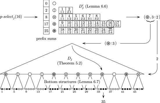
Figure 2: An example evaluation of $\hbox{{p-select\/}}_{j}$ for some color $j$ with the combined data structure of Theorem 6.14. First the argument of $\hbox{{p-select\/}}_{j}$, 16, is translated by $D^{\prime}_{j}$ to the triple $(3,3,2)$ (shown as ($\mskip 1.0mu\lower 0.0pt\hbox{\epsfbox{weight.eps}}\mskip 1.0mu,\mskip 2.0mu$3$\mskip 2.0mu:\mskip 2.0mu$2)) consisting of the relevant weight, $\hbox{$\lower 0.0pt\hbox{\epsfbox{weight.eps}}\mskip 1.0mu$}=3$, the index, 3, of the relevant segment of weight 3 among all segments of weight 3, and the index, 2, of the relevant element within that segment. Then the relevant segment is identified with the aid of $D_{j}$, and finally the relevant element in that segment is located with the corresponding bottom structure, expressed in the form of its global index, 35, and returned. In the interest of clarity, the figure assumes that the $\hbox{{p-select\/}}_{3}$ function of $D_{j}$ in fact coincides with $\hbox{{select\/}}_{3}$.

Computing $N$ as a positive integer with $N=\Theta(t(\log n)^{2})$, we partition the $n$ color values to be maintained into $m=\lceil{n/N}\rceil$ segments of $N$ color values each, except that the last segment may be smaller, and maintain each segment in an instance of the data structure of Lemma 6.12 called a bottom structure. The total number of bits occupied by all bottom structures is $m(N\log c+O({{cN\log N}/{(rt)}}+(\log N)^{2}+1))=n\log c+O({{cn\log(t\log n)}/{(rt)}})=n\log c+O({{cn\log c\log(t\log n)}/{(t\log n)}})$, plus $O(c^{r})=O(n^{\epsilon})$ bits for shared tables.

For each color $j\in\{0,\ldots,c-1\}$, define the $j$-weight of each segment as the number of elements of color $j$ in the segment. We maintain the $j$-weights of all segments in an instance $D_{j}$ of the data structure of Theorem 5.3, with the $j$-weights playing the role of the colors in $D_{j}$. Thus $D_{j}$ is initialized for universe size $m$ and $N+1$ colors. With $a_{i}$ equal to the number of elements of color $j$ in segments of $j$-weight $i$, for $i=0,\ldots,N$, we also maintain the sequence $(a_{0},\ldots,a_{N})$ in an instance $D^{\prime}_{j}$ of the searchable prefix-sum structure of Lemma 6.10, initialized with sum bit length $b=\lceil\log(n+1)\rceil$ and update bit length $\delta=\lceil\log(N+1)\rceil$. As in the previous proof, $D_{0}$ and $D^{\prime}_{0}$ must be treated slightly differently. The total number of bits occupied by $D_{0},D^{\prime}_{0},\ldots,D_{c-1},D^{\prime}_{c-1}$ is $O(c(m+N)\log(m+N)+cN\log n)=O({cn/{(t\log n)}})$. As described at the end of Section 4, we use an additional choice dictionary $D^{*}$ with universe size $m+c$ and therefore negligible space requirements to keep track of and carry out the initialization of the bottom structures and $D_{0},D^{\prime}_{0},\ldots,D_{c-1},D^{\prime}_{c-1}$ as appropriate.

A color query can be answered in constant time by the relevant bottom structure. Because $t\geq\log n$ or $\log N=O(\log w)$, every operation of a bottom structure executes in $O(t)$ time. When a call of setcolor changes the color of an element, from $j_{0}$ to $j$, say, this can be recorded in the relevant bottom structure in $O(t)$ time, after which the update must be reflected in $D_{j_{0}}$, $D_{j}$, $D^{\prime}_{j_{0}}$ and $D^{\prime}_{j}$. Since each of the two weight changes is by 1 or $-1$, each of the updates of $D_{j_{0}}$ and $D_{j}$ can happen in constant time—from the perspective of $D_{j_{0}}$ and $D_{j}$, a color changes into a neighboring color. Similarly, in each of $D^{\prime}_{j_{0}}$ and $D^{\prime}_{j}$, the update changes two values in the sequence maintained, each by at most $N$. A change of this magnitude is covered by the update bit length of $D^{\prime}_{j_{0}}$ and $D^{\prime}_{j}$, and the update can be executed in $O(1+{{\log N}/{\log(1+{w/\delta})}})=O(t)$ time.

Consider a call $\hbox{{p-select\/}}_{j}(k)$ with $j\in\{0,\ldots,c-1\}$ and $k\in\{1,\ldots,n\}$ (Fig. 2). In the sequence $(a_{0},\ldots,a_{N})$ maintained by $D^{\prime}_{j}$, each element $a_{i}$ can be thought of as representing $a_{i}$ elements of the top-level universe $U=\{1,\ldots,n\}$, namely precisely those that have color $j$ and are located in segments of $j$-weight $i$. In particular, $a_{i}$ is always a multiple of $i$. Provided that $k\leq\sum_{i=0}^{N}a_{i}$, $k$ designates a particular element $\ell\in U$ of color $j$ in a natural way: First $i=D^{\prime}_{j}.\hbox{{search\/}}(k)$ selects a particular $j$-weight, $i$, as the weight of $\ell$. Then $p=k-D^{\prime}_{j}.\hbox{{sum\/}}(i-1)$ is the index of $\ell$ in the sequence of all elements of $U$ of color $j$ in segments of $j$-weight $i$, and finally $q=\lceil{p/i}\rceil$ is the index of the segment that contains $\ell$, among those of $j$-weight $i$, and $p-(q-1)i$ is the index of $\ell$ within that segment. Here “index” is to be understood as relative to the orders imposed by the operation $\hbox{{p-select\/}}_{i}$ in $D_{j}$ and the operation $\hbox{{select\/}}_{j}$ in the relevant bottom structure. Altogether, the top-level call $\hbox{{p-select\/}}_{j}(\ell)$ reduces to one call of each of search and sum in $D^{\prime}_{j}$, one call of p-select in $D_{j}$, and one call of select in a bottom structure. It can therefore be executed in $O(t)$ time.

To execute $\hbox{{p-rank\/}}(\ell)$ for $\ell\in U$, we first consult the relevant bottom structure to find the color $j$ of $\ell$ and the index $k$ of $\ell$ among the elements of color $j$ in its segment $R$. Then $D_{j}$ is queried for the $j$-weight $i$ of $R$ and the index $q$ of $R$ among the segments of $j$-weight $i$. Finally the return value is obtained as $D^{\prime}_{j}.\hbox{{sum\/}}(i-1)+(q-1)i+k$. The procedure works in $O(t)$ time.

To equip the data structure with robust iteration, we “plant” $c$ additional instances of the choice dictionary of Theorem 5.3, one for each color, on top of the bottom structures and appeal to the general trie-combination method of Section 4.

Let us now drop the assumption that the tables $Y_{\mbox{\scriptsize E}}$, $Y^{-1}_{\mbox{\scriptsize E}}$, $Y_{\mbox{\scriptsize R}}$ and $Y_{\mbox{\scriptsize S}}$ are available for free. As in the proof of Lemma 6.12, define $\overline{r}=\lceil\sqrt{{r/2}}\rceil$ and $r^{\prime}=\overline{r}^{2}$.

Recall that the task of $Y_{\mbox{\scriptsize E}}$ is to map loose representations of sequences of $r^{\prime}$ small digits to big digits in an arbitrary bijective manner and that $Y^{-1}_{\mbox{\scriptsize E}}$ should realize the inverse mapping. We compute $Y_{\mbox{\scriptsize E}}$ and $Y^{-1}_{\mbox{\scriptsize E}}$ in a lazy fashion that combines techniques used already in the proofs of Lemmas 3.1 and 5.1. We begin by setting $Y_{\mbox{\scriptsize E}}[0]:=0$ and $Y^{-1}_{\mbox{\scriptsize E}}[Y_{\mbox{\scriptsize E}}[0]]:=0$ and initializing an integer $\mu$ to 0. Subsequent loose representations are mapped to the big digits $1,2,\ldots$ in the order in which they present themselves to the encoding table. More precisely, in order to compute the big digit corresponding to a loose representation $a$, we first check whether $a$ was mapped previously in the same manner. This is the case if $0\leq Y_{\mbox{\scriptsize E}}[a]\leq\mu$ and $Y^{-1}_{\mbox{\scriptsize E}}[Y_{\mbox{\scriptsize E}}[a]]=a$. If so, the big digit corresponding to $a$ is simply $Y_{\mbox{\scriptsize E}}[a]$. Otherwise $\mu$ is incremented, and the new value of $\mu$ becomes the big digit corresponding to $a$, a fact recorded by executing $Y_{\mbox{\scriptsize E}}[a]:=\mu$ and $Y^{-1}_{\mbox{\scriptsize E}}[Y_{\mbox{\scriptsize E}}[a]]:=a$. It is easy to see that whenever an entry in $Y^{-1}_{\mbox{\scriptsize E}}$ is inspected by the data structure of Lemma 6.12, it has already been computed (only encoded values are decoded).

$Y_{\mbox{\scriptsize R}}$ and $Y_{\mbox{\scriptsize S}}$ are also provided in a lazy fashion, but present minor additional technical difficulties. We in fact realize $Y_{\mbox{\scriptsize R}}$ and $Y_{\mbox{\scriptsize S}}$ not as tables, but as constant-time functions that carry out two table lookups each.

Recall that $Y_{\mbox{\scriptsize R}}$ operates on “binarized” loose representations of big digits, ones in which all occurrences of a color $j$ of interest have been replaced by 1 and all occurrences of colors other than $j$ have been replaced by 0, with each such value stored in a field of $\lceil\log c\rceil$ bits. Correspondingly, define a big vector to be a sequence of $r^{\prime}$ fields, each of $\lceil\log c\rceil$ bits and containing a value drawn from $\{0,1\}$, and view a big vector as composed of $\overline{r}$ blocks of $\overline{r}$ fields each. After a slight redefinition, the task of $Y_{\mbox{\scriptsize R}}$ is to map each pair $(a,p)$, where $a$ is a big vector and $p\in\{1,\ldots,r^{\prime}\}$, to the sum of the $p$ first fields in $a$. We divide this task into two subtasks: sum the fields in the first $i-1$ blocks in $a$, where $i=\lceil{p/{\overline{r}}}\rceil$; and sum the first $p-(i-1)\overline{r}$ fields in the $i$th block in $a$.

The first subtask is solved with a table $Y^{(1)}_{\mbox{\scriptsize R}}$: For each big vector $a$, $Y^{(1)}_{\mbox{\scriptsize R}}[a]$ is the sequence $(n_{1},\ldots,n_{\overline{r}})$, where $n_{i}$ is the sum of the fields in the $i$ first blocks in $a$, for $i=1,\ldots,\overline{r}$. Thus $Y^{(1)}_{\mbox{\scriptsize R}}$ is a table of sequences of prefix sums. Note that each sequence is of $O(\overline{r}\log r^{\prime})=O(w)$ bits, so that it can be handled in constant time (this is the reason for introducing $\overline{r}$). Each use of the table needs only a single prefix sum that must be picked out from the full sequence. This organization of the table ensures that it can be computed in a lazy fashion: Each color change leads to at most two new big vectors, the entry in $Y^{(1)}_{\mbox{\scriptsize R}}$ of each of which can be computed in constant time using word parallelism from an old entry. The second subtask is handled in a very similar way using a second table $Y^{(2)}_{\mbox{\scriptsize R}}$.

The task of $Y_{\mbox{\scriptsize S}}$ is to map each pair $(a,k)$, where $a$ is a big vector and $k\in\{1,\ldots,r^{\prime}\}$, to the position of the $k$th 1 in $a$, if any. Again the task is divided into two subtasks, each of which is handled in constant time. For the first subtask, we find the number $i$ of the block in $a$ that contains the $k$th 1—assume for simplicity that there is such a block—by computing $i=\hbox{{rank\/}}(k-1,Y^{(1)}_{\mbox{\scriptsize R}}[a])+1$ with the algorithm of Lemma 3.3(d). Let $n_{i-1}$ be the $(i-1)$th number in the sequence $Y^{(1)}_{\mbox{\scriptsize R}}[a]$ (0 if $i=1$). For the second subtask, we have to locate the $(k-n_{i-1})$th 1 in the $i$th block of $a$. This can be done in a similar way using $Y^{(2)}_{\mbox{\scriptsize R}}$ in place of $Y^{(1)}_{\mbox{\scriptsize R}}$.

One may remark that the $O(c\log n)$ bits required to carry out robust iteration are already contained in the bound of the theorem except in the extreme case $t=\Omega({n/{\log n}})$.

If only p-select and not p-rank is to be supported (e.g., if the only goal is to realize the operation uniform-choice), it is possible to avoid the use of Lemma 6.10 for $t=(\log n)^{O(1)}$. In the context of Theorem 6.14 and with $N$ and $\delta$ defined as in its proof, the “bottom” instances of the data structure of Lemma 6.10 (those incorporated, via Lemma 6.12, in the bottom structures in the proof of Theorem 6.14 and in Fig. 2) can easily be replaced by tries of constant height of data structures that maintain the prefix sums directly, realize update via a multiplication by $1_{N,\delta}$, two shifts and an addition, and execute search with the algorithm of Lemma 3.3(d). In slightly greater generality, this method yields a constant-time searchable prefix-sums structure that maintains a sequence of $N+1$ integers, each drawn from $\{0,\ldots,N\}$, under arbitrary updates of single sequence elements. Let us call such a structure an $N$-structure.

For the “top” instances $D^{\prime}_{j}$ in the proof of Theorem 6.14 and in Fig. 2, avoiding Lemma 6.10 is more involved. We sketch the construction. The essential task of a top instance $D^{\prime}_{j}$ can be viewed as that of maintaining a set of $s\leq n$ indistinguishable items, each with a weight in $\{0,\ldots,N\}$ (put differently, a multiset of weights), under insertion and deletion of some (arbitrary) item with a given weight and an operation p-select that maps each argument $k\in\{1,\ldots,s\}$ to the pair $(i,p)$, where $i$ is the weight of the $k$th item and $p$ is its index within the set of items of weight $i$, for some ordering of the items. A first solution to this problems stores the items of weight $i$ in a doubly-linked list $L_{i}$, for $i=0,\ldots,N$, and marks each list item with its weight and its distance to the end of its list. The $N+1$ lists are stored compactly together in an array $A$ of $s$ cells, each of $\Theta(\log n)$ bits, and the positions in $A$ of the first items in each list are recorded in a second array. A new item of weight $i$ is stored in the first free cell in $A$ and inserted at the beginning of $L_{i}$ and computes its distance-to-end value as one more than that of the formerly first item in $L_{i}$. To delete an item of weight $i\in\{0,\ldots,N\}$, we first swap the first item in $L_{i}$ with the item stored in the last used cell in $A$ and then delete it, which does not upset the distance-to-end value of any other item. To execute $\hbox{{p-select\/}}(\ell)$, simply return the pair of the weight and one more than the distance-to-end value of the item in $A[\ell]$.

Assume $n\geq 2$. In order to reduce the space requirements per color from $O(n\log n)$ to $O({n/{(t\log n)}})$, we aggregate the $s$ items into superitems of $N$ items of a common weight each, with up to $N-1$ items left over for each weight in $\{0,\ldots,N\}$. We store the numbers of left-over items for each weight in an $N$-structure $D_{\mbox{\scriptsize L}}$. The superitems are maintained in $N+1$ lists as described above. Since their number is $O({n/N})$, the total number of bits used is indeed $O({n/{(t\log n)}})$. Consider an execution of $\hbox{{p-select\/}}_{j}(k)$, where $j$ is the color under consideration, and let $n_{\mbox{\scriptsize L}}=D_{\mbox{\scriptsize L}}.\hbox{{sum\/}}(N)$ be the total number of left-over items. If $k\leq n_{\mbox{\scriptsize L}}$, compute $i=D_{\mbox{\scriptsize L}}.\hbox{{search\/}}(k)$ and return the pair $(i,k-D_{\mbox{\scriptsize L}}.\hbox{{sum\/}}(i-1))$ as for the original top-level structure $D^{\prime}_{j}$. Otherwise, with $k^{\prime}=k-n_{\mbox{\scriptsize L}}$, let $(i,p)$ be the pair returned by the list-based structure, called with argument $\lceil{{k^{\prime}}/N}\rceil$, and return the pair $(i,(p-\lceil{k^{\prime}}/N\rceil)N+k^{\prime})$. Thus the left-over items are numbered before the items in superitems, and the global number of an item in a superitem is $n_{\mbox{\scriptsize L}}$ plus $N$ times the number of superitems before its own superitem plus its number within the superitem.

7 Nonsystematic Choice Dictionaries

In this section we describe our most space-efficient but also most complicated choice dictionaries. We first consider the (somewhat easier) case in which the number $c$ of colors is a power of 2—until and including Theorem 7.11—and subsequently detail the changes necessary to cope with general values of $c$.

As the reader may recall from the introduction, the game is basically one of squeezing navigational information into the leaves of a tree. Lemma 7.1 below describes a leaf that can be in either the standard representation, which offers no potential for storing additional information, or the ${\bar{j}}$-free representation for some color ${\bar{j}}$ that happens not to be represented at the leaf. In the latter case, information pertaining to the tree path that ends at the leaf can be stored in the leaf together with the usual information kept there. The proof of the central Lemma 7.3 describes how to combine many such leaves to obtain a tree that supports the operations color, setcolor and successor. We first address the overall data organization of the tree and then discuss how to navigate in the tree, after which the implementation of the query operations color and successor is fairly straightforward. The final part of the proof of Lemma 7.3 describes how to re-establish the data-representation invariants of the tree after a call of the update operation setcolor. Lemma 7.9 essentially shows how to put many such trees next to each other to cover a larger universe, and Theorem 7.11 finally obviates the need for precomputed tables.

In the following, let $f$ and $t$ be given positive integers, take $w^{\prime}={w/f}$ and $c=2^{f}$, assume that $d={w/{(2c^{2}ft)}}$ is an integer and at least 2 and let $N=d^{t}$.

Lemma 7.1.

There is a choice dictionary $D$ with universe size $w^{\prime}$ and for $c$ colors that can be initialized in constant time and subsequently occupies $w$ bits and executes color and setcolor in $O(f)$ time and successor in $O(c)$ time. Moreover, during periods in which $S_{\bar{j}}=\emptyset$, where $(S_{0},\ldots,S_{c-1})$ is $D$’s client vector and ${\bar{j}}\in\{0,\ldots,c-1\}$, $D$ supports two additional operations that execute in $O(c)$ time: Conversion from the (initial) standard representation to the ${\bar{j}}$-free representation and conversion back to the standard representation. When $D$ is in the ${\bar{j}}$-free representation, ${\bar{j}}$ must be supplied as an additional argument in calls of color, setcolor and successor and in requests for conversion to the standard representation (we will, however, suppress this in our notation). In return, the $cdt$ bits of the ${\bar{j}}$-free representation of $D$ whose positions are multiples of $2cf$ are unused, i.e., free to hold unrelated information.

Alternatively, for arbitrary fixed $\epsilon>0$, if given access to tables of $O(c^{\epsilon c^{2}})$ bits that can be computed in $O(c^{\epsilon c^{2}})$ time and depend only on $c$, $D$ can execute color, setcolor and successor in constant time.

Proof 7.2.

We can view $D$’s task as that of maintaining a sequence of $w^{\prime}$ digits to base $c$. The standard representation is simply the concatenation, in order, of the $f$-bit binary representations of the $w^{\prime}$ digits. With this representation, the operations can be carried out as for the data structure of Lemma 5.5.

For each ${\bar{j}}\in\{0,\ldots,c-1\}$, the ${\bar{j}}$-free representation partitions the $w^{\prime}$ digits into big groups of $2c^{2}$ consecutive digits each and stores each big group in $(2cf-1)c$ rather than $2c^{2}f$ bits, leaving free every bit whose position is a multiple of $2cf$, as promised in the lemma. First, using the increasing bijection $\hbox{{skip\/}}_{\bar{j}}$ from $\{0,\ldots,c-1\}\setminus\{{\bar{j}}\}$ to $\{0,\ldots,c-2\}$, the $2c^{2}$ digits to base $c$ of each big group are transformed into $2c^{2}$ digits to base $c-1$. Call this the ${\bar{j}}$-intermediate representation. Then the $2c^{2}$ transformed digits are partitioned into $2c$ small groups of $c$ consecutive digits each, and each small group is viewed as a $c$-digit integer written to base $c-1$ and is represented in binary in $cf-1$ bits, which is possible because $c\log(c-1)=c\log c+c\log(1-{1/c})\leq cf+c\ln(1-{1/c})\leq cf-1$. At this point, within each big group, the $2c$ bits whose positions are multiples of $cf$ are unused. For $j=0,\ldots,c-2$, we store in the $(2j+1)$st such bit a summary bit equal to 1 exactly if the color $\hbox{{skip\/}}^{-1}_{{\bar{j}}}(j)$ occurs as a transformed digit in the big group. The summary bits are redundant, but help us to execute successor in constant time. One bit is wasted, and the other half of the $2c$ bits are the promised free bits.

In order to convert $D$ from the standard to the ${\bar{j}}$-free representation, for some ${\bar{j}}\in\{0,\ldots,c-1\}$ with $S_{\bar{j}}=\emptyset$, first the function $\hbox{{skip\/}}_{\bar{j}}$ is applied independently to each digit. Say that the $f$ consecutive bits in which a digit is stored form a field. By Lemma 3.3(c), we can compute an integer $z$, each of whose fields stores 1 if the corresponding digit is $\leq{\bar{j}}$ and 0 otherwise. The function $\hbox{{skip\/}}_{\bar{j}}$ can now be applied in parallel to all fields by a subtraction of $1_{w^{\prime},f}-z$. Subsequently, within each small group of $c$ digits, say $a_{0},\ldots,a_{c-1}$, we must convert $\sum_{i=0}^{c-1}a_{i}c^{i}$ to $\sum_{i=0}^{c-1}a_{i}(c-1)^{i}$. Since the digits $a_{i}$ are readily available as the values of $f$-bit fields, this can be done in $O(c)$ time for all small groups using a word-parallel version of Horner’s scheme in a straightforward manner. Finally, for each $j\in\{0,\ldots,c-2\}$, within each big group a summary bit must be computed and stored in the appropriate position within the big group. To this end, first apply the algorithm of Lemma 3.3(c) at most twice, with $k=j$ and, if $j>0$, with $k=j-1$, followed by bitwise Boolean operations, to obtain an integer in which the most significant digit of each big group is zero, while the remaining bits of the big group are also zero if and only if the digit $j$ does not occur in the big group. A subtraction from $1_{{{w^{\prime}}/{(2c^{2})}},2c^{2}f}\ll(2c^{2}f-1)$ followed by the computation of and and xor with the same number and a suitable shift finishes the computation.

For the conversion in the other direction, i.e., the conversion from $\sum_{i=0}^{c-1}a_{i}(c-1)^{i}$ to $\sum_{i=0}^{c-1}a_{i}c^{i}$ within each small group, after clearing the bits whose positions are multiples of $cf$ (those that held summary and extraneous bits), we compute the digits $a_{0},\ldots,a_{c-1}$ by repeatedly obtaining the remainder modulo $c-1$, which yields the next digit, and keeping only the integer part of the quotient with $c-1$. Except for the division by $c-1$ with truncation, the necessary steps are easily carried out in constant time per digit and $O(c)$ time altogether. Since division is not readily amenable to word parallelism, we replace division by $c-1$ by multiplication by its approximate inverse. More precisely, we carry out the division in constant time using the relation $\lfloor a/{(c-1)}\rfloor=\lfloor{{a\cdot\lceil{{c^{2c}}/{(c-1)}}\rceil}/{c^{2c}}}\rfloor$. To see the validity of the relation for all integers $a$ with $0\leq a<c^{c}$, simply observe that ${a/{(c-1)}}\leq{{a\cdot\lceil{{c^{2c}}/{(c-1)}}\rceil}/{c^{2c}}}<{a/{(c-1)}}+{1/{c^{c}}}<{{(a+1)}/{(c-1)}}$ and note that there is no integer strictly between ${a/{(c-1)}}$ and ${{(a+1)}/{(c-1)}}$. The product $a\cdot\lceil{{c^{2c}}/{(c-1)}}\rceil$ may have more than $cf$ bits. It has no more than $3cf$ bits, however, so it can be computed using “triple precision”, which we simulate by handling the small groups in three rounds, each round operating only on every third group. Truncated division by $c^{2c}$ is, of course, realized as a right shift by $2cf$ bit positions followed by a “masking away” of the unwanted bits. At the very end, to get from the ${\bar{j}}$-intermediate to the standard representation, $\hbox{{skip\/}}^{-1}_{\bar{j}}$ must be applied independently to each field. This can be done similarly as described above for $\hbox{{skip\/}}_{\bar{j}}$.

As detailed above, the conversion between the standard and the ${\bar{j}}$-intermediate representations depends on ${\bar{j}}$, but takes only constant time. In contrast, the conversion between the ${\bar{j}}$-intermediate and the ${\bar{j}}$-free representations takes $\Theta(c)$ time, but is independent of ${\bar{j}}$. This observation is important to the proof of Theorem 7.11.

Assume that $D$ is in the ${\bar{j}}$-free representation, for some ${\bar{j}}\in\{0,\ldots,c-1\}$, and that a call $\hbox{{successor\/}}(j,\ell)$ is to be executed for some $j\in\{0,\ldots,c-1\}\setminus\{{\bar{j}}\}$ and $\ell\in\{0,\ldots,w^{\prime}-1\}$. Suppose, for ease of discussion, that the return value $\ell^{\prime}$ is nonzero, and let $G$ and $G^{\prime}$ be the big groups that contain the $(\ell+1)$st and the $(\ell^{\prime})$th digit, respectively. Applying to $G$ a computation that, informally, converts the single big group $G$ to the standard representation, we can test whether the $(\ell^{\prime})$th digit belongs to $G$ and, if so, find and return $\ell^{\prime}$. Otherwise we locate $G^{\prime}$ by applying an algorithm of Lemma 3.3(a) to a suitable suffix of those summary bits that pertain to the color $j$, with all other bits cleared, after which $\ell^{\prime}$ can be found by converting $G^{\prime}$ to the standard representation as done previously for $G$. The computation runs in $O(c)$ time, its bottleneck being the conversions to the standard representation. It is easy to see that color and setcolor can be executed in $O(f)$ time by computing the relevant power of $c$ via repeated squaring.

Alternatively, the conversion of single big groups from the ${\bar{j}}$-intermediate to the ${\bar{j}}$-free representation and vice versa can be carried out by table lookup. A table for each direction of the conversion maps each sequence of $c^{2}$ possible digits to the corresponding other representation and therefore has $O(c^{c^{2}})$ entries of $O(c^{2}f)$ bits each. For fixed $\epsilon>0$ and for $c$ larger than a suitable constant, we can instead use repeated table lookup, mapping at most ${{\epsilon c}/2}$ small groups of $c$ digits each at a time. This reduces the number of bits in the tables and the time needed to compute them to $O(c^{3+{{\epsilon c^{2}}/2}})=O(c^{\epsilon c^{2}})$. In the case of the conversion to the ${\bar{j}}$-free representation, each table entry for at most ${{\epsilon c}/2}$ small groups must provide suitable summary bits for the small groups concerned, and the composition of such entries includes forming the bitwise or of the partial summaries.

Lemma 7.3.

There is a choice dictionary $D$ with universe size $Nw^{\prime}$ and for $c$ colors that can be initialized in constant time, uses $Nw+2$ bits and supports color in $O(t+f)$ time and setcolor and successor in $O(t+c)$ time.

Alternatively, for arbitrary fixed $\epsilon>0$, if given access to tables of $O(c^{\epsilon c^{2}})$ bits that can be computed in $O(c^{\epsilon c^{2}})$ time and depend only on $c$, $D$ can execute color and successor in $O(t)$ time.

Proof 7.4.

Let $T=(V,E)$ be a complete $d$-ary outtree of depth $t$, whose leaves, in the order from left to right, we will identify with the integers $1,\ldots,N$. Let $r$ be the root of $T$ and, for all $u\in V$, take $T_{u}$ to be the maximal subtree of $T$ rooted at $u$.

Let the client vector of $D$ be $(S_{0},\ldots,S_{c-1})$. We divide the universe $U=\{1,\ldots,Nw^{\prime}\}$ into $N$ segments $U_{1},\ldots,U_{N}$ of $w^{\prime}$ consecutive integers each. For each $u\in V$, call $u$ full if $S_{j}\cap U_{i}\not=\emptyset$ for all $j\in\{0,\ldots,c-1\}$ and all leaf descendants $i$ of $u$, and deficient otherwise. Informally, a deficient node is one that has a leaf descendant with a missing color. For each $u\in V$, let the spectrum of $u$ be the string $b_{0}\cdots b_{c-1}$ of $c$ bits defined as follows: If $u$ is deficient, then for $j=0,\ldots,c-1$, $b_{j}=1$ exactly if $S_{j}\cap U_{i}\not=\emptyset$ for some leaf descendant $i$ of $u$ (informally, if the color $j$ is represented in $T_{u}$). If $u$ is full, as a special convention, $b_{0}\cdots b_{c-1}=0\cdots 0$, a bit combination that cannot otherwise occur. If $b_{0}\cdots b_{c-1}=100\cdots 0$ (only the color 0 is represented in $T_{u}$), we say that $u$ is empty; this is initially the case for every node $u$. If a node in $T$ is deficient but not empty, we call it light. For each inner node $u$ in $T$, define the navigation vector of $u$ to be the concatenation $\gamma_{1}\cdots\gamma_{d}$, where $\gamma_{1},\ldots,\gamma_{d}$ are the spectra of the $d$ children of $u$ in the order from left to right.

For $i=1,\ldots,N$, let $\mathcal{P}^{\prime}_{i}$ be the semipartition $(S_{0}\cap U_{i},\ldots,S_{c-1}\cap U_{i})$ of $U_{i}$ and let $\mathcal{P}_{i}$ be the semipartition of $\{1,\ldots,w^{\prime}\}$ obtained from $\mathcal{P}^{\prime}_{i}$ by subtracting $(i-1)w^{\prime}$ from every element in each of its sets. We do not store $T$. Instead, for $i=1,\ldots,N$, $\mathcal{P}_{i}$ is stored in an instance $D_{i}$ of the choice dictionary of Lemma 7.1 called a leaf dictionary, and $D_{1},\ldots,D_{N}$ are in turn stored in $N$ words $H_{1},\ldots,H_{N}$ of $w$ bits each. Two additional root bits indicate whether the root $r$ of $T$ is full and whether it is empty. It is helpful to think of $H_{i}$ as “normally” storing $D_{i}$, for $i=1,\ldots,N$. If this were always the case and all navigation vectors were available, a call of $\hbox{{successor\/}}(j,\ell)$ could essentially use navigation vectors to find a path from $r$ to the leftmost leaf $i$ in $T$ such that $S_{j}\cap U_{i}$ contains an element larger than $\ell$, if any, and the smallest such element could be obtained through a call of $D_{i}.\hbox{{successor\/}}$. Moreover, setcolor could update navigation vectors as appropriate. However, we have no space left to store navigation vectors, and so have to proceed differently.

The parent of every light node in $T$ other than $r$ is also light, and every deficient inner node in $T$ has at least one deficient child. Let the preferred child of a deficient inner node be its leftmost light child if it has at least one light child, and its leftmost empty child otherwise. Let $Q=(V_{Q},E_{Q})$ be the subgraph of $T$ induced by the edge set $E_{Q}$ obtained as follows: First include in $E_{Q}$ all edges from a light inner node to its preferred child. Then, for every empty node $v$ that has an incoming edge in $E_{Q}$, include in $E_{Q}$ the edges on the path from $v$ to its leftmost leaf descendant. $Q$ is a collection of node-disjoint paths called light paths, each of which ends at a leaf in $T$. When $P$ is a light path that starts at a (light) node $u$ and ends at a (deficient) leaf $v$, we call $u$ the top node, $v$ the proxy and the leftmost leaf descendant of $u$ (that may coincide with $v$) the historian of $P$ and of every node on $P$. A light node in $T$ that is neither the root nor a leaf is a top node exactly if it is not the preferred child of its parent, i.e., if it has at least one light left sibling. No proper ancestor of a top node $u$ can have a descendant of $u$ as its leftmost leaf descendant, so a leaf is the historian of at most one light path. If $h$ is the historian of a light path $P$, the top node and the proxy of $P$ are also said to be the top node and the proxy, respectively, of $h$. These concepts are illustrated in Fig. 3. A leaf $i$ cannot be the historian of one light path and the proxy of another, since otherwise the two corresponding top nodes would both be ancestors of $i$ and the path between them would contain only gray nodes and be part of a light path, an impossibility. A similar argument shows that in the left-to-right order of the leaves of $T$, no historian or proxy lies strictly between a historian and its proxy.

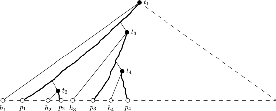
Figure 3: Example light paths (drawn thicker). Top nodes, historians and proxies are labeled “$t$”, “$h$” and “$p$”, respectively, and a subscript identifies the associated light path.

Suppose that the nodes on a light path $P$ are $u_{1},\ldots,u_{k}$, in that order. Then the history of $P$ and of each of $u_{1},\ldots,u_{k}$ is the concatenation of the navigation vectors of $u_{1},\ldots,u_{k-1}$, in that order ($u_{k}$, as a leaf, has no navigation vector). An important fact to note is that if a leaf dictionary is in the ${\bar{j}}$-free representation for some ${\bar{j}}\in\{0,\ldots,c-1\}$, then it allows the history of a light path to be stored in its $cdt$ free bits. In order for this actually to be possible, we assume that histories (and, by extension, navigation vectors and spectra) are represented with gaps of $2cf-1$ bit positions between consecutive bits, so that a history spreads over up to an entire $w$-bit word. To fill up the word, we store a history of $cdk$ bits prefixed by $cd(t-k)$ arbitrary bits, so that the positions in the word of the bits that make up the navigation vector of a node $u$ depend only on the height of $u$.

We represent $(S_{0},\ldots,S_{c-1})$ using the following storage scheme: Let $\pi$ be the permutation of $\{1,\ldots,N\}$ that maps each $i\in\{1,\ldots,N\}$ to itself, except that $\pi(p)=h$ and $\pi(h)=p$ for each pair of a proxy $p$ and its historian $h$. Then the following holds for $i=1,\ldots,N$: $D_{i}$ is stored in $H_{\pi(i)}$, and

• if $i$ is a proxy (and therefore deficient), $D_{i}$ is in the ${\bar{j}}$-free representation, where ${\bar{j}}=\min\{j\in\mathbb{N}_{0}\mid 0\leq j\leq c-1$ and $S_{j}\cap U_{i}=\emptyset\}$—we will say that $D_{i}$ is in the compact representation—and $H_{\pi(i)}$ stores not only $D_{i}$, but also the history of $i$;

• if $i$ is empty but not a proxy, $D_{i}$ may not have been initialized; equivalently, $H_{\pi(i)}$ may hold an arbitrary value;

• in all remaining cases, i.e., if $i$ is neither a proxy nor empty, $D_{i}$ is in the standard representation.

This paragraph tries to motivate the not-so-natural storage scheme. The usefulness of navigation vectors was already observed above. All nontrivial navigation vectors are contained in the histories of the proxies. As we have seen, if $p$ is a proxy and therefore deficient, $\mathcal{P}_{p}$ can be represented sufficiently compactly to allow the history of $p$ to be stored with it. However, when the history of a proxy $p$ is needed, $p$ is not known, so $H_{p}$ cannot be located. The top node of $p$ and hence also the historian $h$ of $p$ are known, however, so we store $D_{p}$ and the history of $p$ in $H_{h}$ rather than in $H_{p}$. In return (unless $h=p$), $H_{p}$ must hold (the standard representation of) $D_{h}$. The terms “historian” and “proxy” serve as reminders that a historian (more precisely, the corresponding storage word) holds a history (namely that of its proxy), whereas a proxy holds the data of what may be another leaf (namely of its historian). The convention that $H_{i}$ may be arbitrary if $i$ is an empty leaf that is not in use as a proxy is necessary to guarantee a constant initialization time.

If we represent a current node in $T$ as suggested in Section 4, i.e., through the triple $(j,k,d^{j})$, where $j$ is the height in $T$ of the current node and $k$ is one more than the number of nodes of height $j$ to its left, we can navigate in $T$ as described in Section 4. One operation that was not considered there and that we need now is computing the leafmost leaf descendant of the current node. This is easy: If the current node is (represented through) $(j,k,d^{j})$, its leftmost leaf descendant in $T$ is $(0,(k-1)\cdot d^{j}+1,1)$.

Proposition 7.5.

Let $u$ and $v$ be inner nodes in $T$ such that $v$ is a child of $u$ and assume that we know the navigation vector of $u$, whether $u\in V_{Q}$ (i.e., whether $u$ belongs to a light path) and, if $u$ is light, its history. Then, in constant time, we can compute the spectrum and the navigation vector of $v$, decide whether $v\in V_{Q}$ and whether $v$ is a top node and, if $v$ is light, compute its history.

Proof 7.6.

The spectrum of $v$ can be read off the navigation vector of $u$. If $v$ is full or empty, its navigation vector is trivial, namely the concatenation of $d$ copies of either $0\cdots 0$ or $100\cdots 0$, $v$ is not a top node, and $v\in V_{Q}$ exactly if $u\in V_{Q}$ and $v$ is $u$’s preferred child. The latter condition can be tested in constant time by inspection of the navigation vector of $u$. Assume now that $v$ is light, so that $v\in V_{Q}$. Then $v$ is a top node exactly if it has at least one light left sibling. If this is the case, the history of $v$ is stored at $v$’s leftmost leaf descendant $h$ (more precisely, in $H_{h}$), from where it can be retrieved in constant time. If $v$ is not a top node, it belongs to the same light path as $u$, whose history is known by assumption. The navigation vector of $v$ can be extracted from $v$’s history in constant time.

Proposition 7.5 provides the general step in an inductive argument to show that we can traverse a root-to-leaf path in $T$ in constant time per edge, always—until a leaf is reached—knowing the navigation vector of the current node, whether it is a top node, whether it belongs to a light path and, except in the case of the root $r$ of $T$, its spectrum. As for the inductive basis, $r$ is a top node and belongs to a light path if and only if $r$ is light, and whether this is the case is indicated by the two root bits. If $r$ is a top node, its history is available in $H_{1}$ and, as above, the navigation vector of $r$ can be extracted from its history in constant time. If $r$ is not a top node, it is full or empty, and its navigation vector is trivial, as above.

Our traversals of root-to-leaf paths in $T$ (called “descents”) will be carried out by starting at $r$ and repeatedly applying a selection rule at the current node $u$ until a leaf is reached. The selection rule indicates the child of $u$ at which the descent is to be continued. We use three different selection rules that we name for easier reference:

“leaf-seeking”$(i)$

($i$ is a leaf descendant of the current node $u$): Step to that child of $u$ that is an ancestor of $i$.

“proxy-seeking”

(the current node $u$ belongs to a light path): Step from $u$ to its preferred child.

“color-seeking”$(j)$

($j\in\{0,\ldots,c-1\}$ and the color $j$ is represented in $T_{u}$, where $u$ is the current node): Step from $u$ to the leftmost child of $u$ in whose spectrum the $(j+1)$st bit is set.

Using algorithms of Lemma 3.3 for the rules “proxy-seeking” and “color-seeking”, we can apply each of the selection rules above in constant time.

The permutation $\pi$ is not explicitly recorded. As the following proposition shows, however, we can compute $\pi(i)$ for arbitrary given $i\in\{1,\ldots,N\}$. What the proposition actually says is that we can compute both $\pi(i)$ and the information necessary to make sense of the contents of $H_{\pi(i)}$.

Proposition 7.7.

Given $i\in\{1,\ldots,N\}$, in $O(t)$ time we can compute $\pi(i)$, the spectrum of $i$, and whether $i$ is a proxy.

Proof 7.8.

Use a first descent in $T$ with the selection rule “leaf-seeking”$(i)$ to determine if $i\in V_{Q}$ and to compute the spectrum of $i$, which will be known when the leaf $i$ is reached. Now $i$ is a proxy exactly if $i\in V_{Q}$. In a second descent in $T$, initially again use the selection rule “leaf-seeking”$(i)$. Starting at the time when the current node is first a top node, if ever, always remember the historian $h$ of the most recently visited top node (the history stored in $H_{h}$ is used for navigational purposes anyway). If and when the current node becomes a top node with $i$ as its leftmost leaf descendant, (this will happen at some point exactly if $i$ is a historian), permanently change the selection rule to “proxy-seeking” and continue the descent. Let $k$ be the leaf reached. If the selection rule is still “leaf-seeking” at this time and $k=i\in V_{Q}$, $i$ is a proxy with historian $h$ and $\pi(i)=h$; otherwise $\pi(i)=k$.

$D$’s operations are implemented as follows:

color: To execute $\hbox{{color\/}}(\ell)$ for $\ell\in\{1,\ldots,Nw^{\prime}\}$, take $i=\lceil{\ell/{w^{\prime}}}\rceil$ and $m=\ell-(i-1)w^{\prime}$. Thus $\ell$ is the $m$th element of the $i$th segment $U_{i}$. Use the algorithm of Proposition 7.7 to compute $\pi(i)$ and the related information. If $i$ is empty, return 0. Otherwise determine whether $D_{i}$ (stored in $H_{\pi(i)}$) is in the ${\bar{j}}$-free representation for some ${\bar{j}}$ and, if so, for which ${\bar{j}}$ (Lemma 3.3(b)). Using the information just computed to consult $D_{i}$, return $D_{i}.\hbox{{color\/}}(m)$.

successor: To execute $\hbox{{successor\/}}(j,\ell)$ for $j\in\{0,\ldots,c-1\}$ and $\ell\in\{1,\ldots,Nw^{\prime}\}$, initially proceed similarly as in the case of color: Take $i=\lceil{\ell/{w^{\prime}}}\rceil$ and $m=\ell-(i-1)w^{\prime}$ and use the algorithm of Proposition 7.7 to compute $\pi(i)$ and the related information. If $i$ is empty, $m<w^{\prime}$ and $j=0$, return $\ell+1$. If $i$ is nonempty, use $D_{i}$ (stored in $H_{\pi(i)}$) to compute $k=D_{i}.\hbox{{successor\/}}(j,m)$ and, if $k\not=0$, return $(i-1)w^{\prime}+k$.

If no value was returned until this point (the answer could not be established locally in the $i$th segment), again traverse the path $P$ in $T$ from $r$ to $i$. With $X$ equal to the set of right siblings $u$ of inner nodes on $P$ such that the $(j+1)$st bit is set in $u$’s spectrum, determine whether $X=\emptyset$ and, if so, return 0. Otherwise proceed as follows: Compute the node $u$ in $X$ that follows $i$ most closely in a preorder traversal of $T$ (thus $u$ is the closest right sibling in $X$ of the node on $P$ of maximum depth among those with right siblings in $X$). Carry out a partial descent in $T$ that starts at $u$ and uses the selection rule “color-seeking”$(j)$ throughout. Let $k$ be the leaf reached and use the algorithm of Proposition 7.7 to compute $\pi(k)$ and the related information. If $k$ is empty, return $(k-1)w^{\prime}+1$ (we must have $j=0$). Otherwise use $D_{k}$ (stored in $H_{\pi(k)}$) to return $(k-1)w^{\prime}+D_{k}.\hbox{{successor\/}}(j,0)$.

setcolor: Let us use the terms “old” and “new” to refer to states before and after the update under consideration, respectively. To execute $\hbox{{setcolor\/}}(j,\ell)$ for $j\in\{0,\ldots,c-1\}$ and $\ell\in\{1,\ldots,Nw^{\prime}\}$, once more take $i=\lceil{\ell/{w^{\prime}}}\rceil$ and $m=\ell-(i-1)w^{\prime}$. Find the old color $j_{0}$ of $\ell$, determine whether $S_{j_{0}}\cap U_{i}=\emptyset$ after the update and use this to compute the new spectrum of $i$. Save the old root bits and traverse the path $P$ in $T$ from $r$ to $i$, collecting the concatenation $\Gamma$ of the navigation vectors of all inner nodes on $P$. Use $\Gamma$ to traverse $P$ backwards and update the histories of all old top nodes encountered and the root bits to reflect the change, if any, in the spectrum of $i$. Since the spectrum of every inner node in $T$ is a simple function of those of its children, this is a straightforward bottom-up computation. Also explicitly compute the concatenation $\Gamma^{\prime}$ of the new navigation vectors of the inner nodes on $P$. Guided by $\Gamma$ and $\Gamma^{\prime}$, we can traverse $P$ in the forward and backward directions in constant time per node visited, always knowing both the old and the new navigation vector of the current node, even though the histories stored in $H$ may be temporarily inconsistent during the update. What remains is to actually record the new color of $\ell$ and to modify the light paths implicit in the values in $H$ accordingly. After describing a procedure for achieving this, we will argue that whenever the procedure needs the (old and new) navigation vector of a node outside of $P$, the navigation vector can be obtained from the history stored in a word that has not (yet) been modified in the course of the update.

We consider three cases. In Case 1 the set of light paths does not change. In Case 2 the update creates a new light path, which may shorten a single existing light path. In Case 3 the update destroys a light path, which may lengthen a single existing light path. The update either leaves invariant the status of every node in $T$ with respect to being empty, light or full, or it causes the same transition from light to empty or full or from empty or full to light at all nodes on a last (bottom) part of $P$, while the other nodes on $P$ remain light and no other node changes its status.

Case 1: $i\in V_{Q}$ is true after the update if and only if it was true before the update.
If the update changes $i$’s status with respect to being empty, light or full, we must have one of two situations: Either $i\not\in V_{Q}$ even when $i$ is light, in which case $i$ has at least one light leaf as a left sibling, or $i\in V_{Q}$ even when $i$ is not light, in which case the status of $i$ switches between light and empty and the light path that ends at $i$ when $i$ is empty coincides with the light path that ends at $i$ when $i$ is light (informally, the switch to light of some nodes on the path but not its first node—which is always light—only makes those nodes “more preferred children”). It is now easy to see that the update does not change the set of light paths.

Use the algorithm of Proposition 7.7 to compute $\pi(i)$ and the related information. If $i$ is a proxy before and therefore also after the update, convert $D_{i}$ (found in $H_{\pi(i)}$) to the standard representation after saving the history stored in its free bits in a temporary variable, then execute $D_{i}.\hbox{{setcolor\/}}(j,m)$, and finally reconvert $D_{i}$ to the compact representation (which may be the ${\bar{j}}$-free representation for a different ${\bar{j}}$) and store the history saved in its free bits. If $i$ was empty but not a proxy before the update, let $D_{i}$ be a newly initialized leaf dictionary, execute $D_{i}.\hbox{{setcolor\/}}(j,m)$ and store $D_{i}$ in $H_{\pi(i)}$. In the remaining case only execute $D_{i}.\hbox{{setcolor\/}}(j,m)$.

Case 2: $i\in V_{Q}$ holds after the update, but not before it.
In this case $i$ is the last node of a new light path $P^{\prime}$. Again traverse $P$ backwards to find the first node $v$ on $P$ (i.e., the node on $P$ of maximum height) that did not belong to a light path before the update. The update changes the status of $i$ and $v$ from empty or full to light. Moreover, after the update every proper descendant of $v$ on $P$ is the only light child of its parent and therefore its preferred child.

If $v$ has at least one light left sibling or is the root $r$ of $T$, $v$ is not a preferred child even after the update and so must be an inner node in $T$, i.e., we cannot have $v=i$ (and nontheless be in Case 2). Then $v$ is the top node of $P^{\prime}$, $i$ is its proxy, and the leftmost leaf descendant $h$ of $v$ is the historian of $P^{\prime}$ (see Fig. 4(a)). Since neither $i$ nor $h$ was the leftmost leaf descendant of a light node in $T$ or belonged to a light path before the update, neither was a proxy or a historian before the update. Thus $\pi$ changes into a permutation $\pi^{\prime}$ of $\{1,\ldots,N\}$ that coincides with $\pi$, except that $\pi(i)=i=\pi^{\prime}(h)$ and $\pi(h)=h=\pi^{\prime}(i)$. Accordingly carry out the following steps: If $i$ was empty before the update, let $D_{i}$ be a newly initialized leaf dictionary. Subsequently, whether or not $i$ was empty, execute $D_{i}.\hbox{{setcolor\/}}(j,m)$ and convert $D_{i}$ to the compact representation. Then store $D_{i}$ together with the new history of $i$, which is a suffix of $\Gamma^{\prime}$, in $H_{h}$ while saving the old value of $H_{h}$ in $H_{i}$ if $h\not=i$.

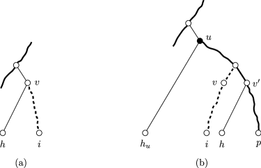
Figure 4: (a) A new light path $P^{\prime}$ (from $v$ to $i$) is added without changes to the existing light paths. (b) A new light path (from $u$ to $i$) grabs an initial part of an old light path (from $u$ to $p$).

If $v$ has no light left sibling and is not $r$, the situation is more complicated (see Fig. 4(b)). This is because the update switches the preferred child of the parent of $v$ from some sibling $v^{\prime}$ of $v$ to $v$. Carry out a partial descent in $T$, starting at $v^{\prime}$ and with the selection rule “proxy-seeking”, to find the end node $p$ of the old light path through $v^{\prime}$ and let $h$ be the leftmost leaf descendant of $v^{\prime}$. Also ascend in $T$ from $v$ until finding the last (deepest) node $u$ on $P$ that was a top node before the update. After the update $u$ is still a top node, but with proxy $i$ instead of its old proxy $p$. Assume first that $v^{\prime}$ is a nonempty inner node in $T$. Then $v^{\prime}$ is a right sibling of $v$ and a new top node with proxy $p$ and historian $h$. Let $h_{u}$ be the historian of $u$ (which does not change as a result of the update). Before the update, $i$ was neither a proxy nor a historian unless $i=h_{u}$, and $h$ was neither a proxy nor a historian unless $h=p$. The update therefore changes $\pi$ into the permutation $\pi^{\prime}$ of $\{1,\ldots,N\}$ that coincides with $\pi$, except that

$\pi(h)$ $=$ $h$ $=$ $\pi^{\prime}(p)$          (only if $h\not=p$) $\pi(p)$ $=$ $h_{u}$ $=$ $\pi^{\prime}(i)$ $\pi(i)$ $=$ $i$ $=$ $\pi^{\prime}(h_{u})$          (only if $i\not=h_{u}$) $\pi(h_{u})$ $=$ $p$ $=$ $\pi^{\prime}(h)\hbox to0.0pt{.\hss}$

Accordingly, move the old value of $H_{h}$ to $H_{p}$ (superfluous if $h=p$), move the old value of $H_{p}$ to $H_{i}$ (superfluous if $i=h_{u}$), let $D_{i}$ be a newly initialized leaf dictionary if $i$ was empty before the update and otherwise obtain $D_{i}$ from the old value of $H_{\pi(i)}$, execute $D_{i}.\hbox{{setcolor\/}}(j,m)$, store the compact representation of $D_{i}$ together with the new history of $i$ (which is a suffix of $\Gamma^{\prime}$) in $H_{h_{u}}$, and finally move the old value of $H_{h_{u}}$ to $H_{h}$. The latter value contains $D_{p}$ together with the old history of $p$. The new history of $p$ is a proper suffix of its old history, but storing the latter does no harm (the extra bits are considered unused anyway).

If $v^{\prime}$ is empty, the steps executed are the same, except that we refrain from moving the old value of $H_{h_{u}}$ to $H_{h}$ (if $h=h_{u}$ the appropriate value was already stored in $H_{h}$, and if $h\not=h_{u}$ the new value of $H_{h}$ can be arbitrary). Finally, if $v^{\prime}$ is a nonempty leaf, the procedure is also the same, except that at the end, since $v^{\prime}=p=h$ stops being a proxy, $D_{p}$ (stored in $H_{p}$) must be converted to the standard representation. Its free bits contain no relevant information.

Case 3: $i\in V_{Q}$ holds before the update, but not after it.
This case essentially entails undoing the steps described for the previous case. Traverse $P$ backwards to find the first node $v$ on $P$ that ceases to belong to $V_{Q}$ as a result of the update. The update changes the status of $i$ and $v$ from light to empty or full.

If $v$ was a top node before the update, $i$ was its proxy, and neither $i$ nor the old historian $h$ of $v$ is a proxy or a historian after the update. Thus $\pi$ changes into the permutation $\pi^{\prime}$ of $\{1,\ldots,N\}$ that coincides with $\pi$, except that $\pi(i)=h=\pi^{\prime}(h)$ and $\pi(h)=i=\pi^{\prime}(i)$. Accordingly obtain $D_{i}$ from $H_{h}$, convert it to the standard representation, execute $D_{i}.\hbox{{setcolor\/}}(j,m)$ and store $D_{i}$ in $H_{i}$ while saving the old value of $H_{i}$ in $H_{h}$ if $h\not=i$.

If $v$ was not a top node before the update, let $v^{\prime}$ be the preferred child of the parent of $v$ after the update and let $h$ be the leftmost leaf descendant of $v^{\prime}$. If $v^{\prime}$ is empty take $p=h$, and otherwise let $p$ be the leaf reached by a partial descent in $T$ that starts at $v^{\prime}$ and uses the selection rule “proxy-seeking”. Assume first that $v^{\prime}$ is a nonempty inner node in $T$. Then $v^{\prime}$ was a top node with proxy $p$ and historian $h$ before the update. Ascend in $T$ from $v$ to find the last node $u$ on $P$ that was a top node before the update. After the update $u$ is still a top node, but with proxy $p$ instead of its old proxy $i$, and $v^{\prime}$ is not a top node. Let $h_{u}$ be the historian of $u$ (which does not change as a result of the update). After the update, $i$ is neither a proxy nor a historian unless $i=h_{u}$, and $h$ is neither a proxy nor a historian unless $h=p$. Therefore the update changes $\pi$ into the permutation $\pi^{\prime}$ of $\{1,\ldots,N\}$ that coincides with $\pi$, except that

$\pi(h)$ $=$ $p$ $=$ $\pi^{\prime}(h_{u})$ $\pi(h_{u})$ $=$ $i$ $=$ $\pi^{\prime}(i)$          (only if $i\not=h_{u}$) $\pi(i)$ $=$ $h_{u}$ $=$ $\pi^{\prime}(p)$ $\pi(p)$ $=$ $h$ $=$ $\pi^{\prime}(h)$          (only if $h\not=p$).

Accordingly, move the old value of $H_{h}$ to $H_{h_{u}}$ after prefixing the history stored in $H_{h}$ by the subsequence of $\Gamma^{\prime}$ that pertains to the part of $P$ from $u$ to the parent of $v^{\prime}$, convert $D_{i}$ (found in the old value of $H_{h_{u}}$) to the standard representation, execute $D_{i}.\hbox{{setcolor\/}}(j,m)$ and store $D_{i}$ in $H_{\pi^{\prime}(i)}$. Finally move the old value of $H_{i}$ to $H_{p}$ if $i\not=h_{u}$ and move the old value of $H_{p}$ to $H_{h}$ if $h\not=p$.

If $v^{\prime}$ is empty, the steps executed are the same, except that in place of the old value of $H_{h}$ (which can be arbitrary) we use a newly initialized leaf dictionary, converted to the compact representation and equipped with a history that shows every node as being empty. If $v^{\prime}$ is a nonempty leaf, the procedure is also the same, except that since $v^{\prime}=h=p$ was not a proxy before the update, the old value of $H_{h}$, before being moved to $H_{h_{u}}$, must be converted to the compact representation and equipped with a history equal to (the empty sequence prefixed by) the subsequence of $\Gamma^{\prime}$ that pertains to the part of $P$ from $u$ to the parent of $v^{\prime}$.

Observe that within each of Cases 1–3, all reading from some of $H_{1},\ldots,H_{N}$ can take place before all writing to some of the same words. Therefore the only possible source of inconsistency in the data read is the update of histories of nodes on $P$ carried out before the computation splits into Cases 1–3. Most of the update conceptually happens on the path $P$, on which we can navigate using $\Gamma$ and $\Gamma^{\prime}$. The only occasion on which we need to navigate outside of $P$ is during the partial descent from $v^{\prime}$ that takes place in Cases 2 and 3. But if $v^{\prime}$ is empty, the descent is trivial and needs no inspection of histories, and if $v^{\prime}$ is light, it is necessarily to the right of $v$, which implies that every history inspected during the descent from $v^{\prime}$ is stored strictly to the right of every history of a node on $P$, and thus of every leaf whose associated word might already have changed.

Every operation of $D$ inspects or changes $O(t)$ parts of histories stored in leaf dictionaries, which takes $O(t)$ time. In addition to this, $D.\hbox{{color\/}}$ calls color once in a leaf dictionary and $D.\hbox{{successor\/}}$ calls successor at most twice in a leaf dictionary. Therefore these operations execute in $O(t+f)$ and $O(t+c)$ time, respectively. $D.\hbox{{setcolor\/}}$ carries out a constant number of conversions between standard and compact representations in leaf dictionaries and therefore altogether executes in $O(t+c)$ time. If tables are available that allow the leaf dictionaries to execute color and successor in constant time, $D$’s operations color and successor work in $O(t)$ time (whereas the time bound for setcolor does not change). This ends the proof of Lemma 7.3.

Lemma 7.9.

There is a choice dictionary that, for arbitrary $n,f,t\in\mathbb{N}$, can be initialized for universe size $n$, $c=2^{f}$ colors and tradeoff parameter $t$ in constant time and that subsequently occupies $nf+O({{cn(c^{2}ft}/w})^{t}+\log n)$ bits and supports color in $O(t+f)$ time and setcolor, choice and, given $O(c\log n)$ additional bits, robust iteration in $O(t+c)$ time.

Alternatively, for arbitrary fixed $\epsilon>0$, if given access to tables of $O(c^{\epsilon c^{2}})$ bits that can be computed in $O(c^{\epsilon c^{2}})$ time and depend only on $c$, the data structure supports color, choice and, given $O(c\log n)$ additional bits, robust iteration in $O(t)$ time.

Proof 7.10.

A data structure composed of $c$ instances of the data structure of Theorem 5.7, one for each color, can support each operation in constant time. Assume therefore without loss of generality that $c^{2}ft<w$. A word RAM with a word length of $w$ bits can simulate one with a word length of $2w$ bits with constant slowdown. This allows us to assume not only that $c^{2}ft<w$, but that $w$ is a multiple of $c^{2}ft$ and that the available word length is in fact $2w$. Therefore define $d={{2w}/{(2c^{2}ft)}}={w/{(c^{2}ft)}}\geq 2$ and $N=d^{t}$ and let $w^{\prime}={{2w}/f}$, in accordance with the conventions used in this section until this point. Define $m=\lceil{n/{(Nw^{\prime})}}\rceil$. If $m=1$, the result follows directly from Lemma 7.3. The latter assumes the universe size to be exactly $Nw^{\prime}$, but a tree with fewer than $N$ leaves can be accommodated with straightforward changes—essentially, each node should adapt to the number of its children—and an “incomplete leaf”, one whose universe size is smaller than $w^{\prime}$, can be handled separately with Lemma 5.5.

If $m\geq 2$, we employ the trie-combination method of Section 4 with the degree sequence $(Nw^{\prime},n)$, so that the overall trie is of height 2. The 2-color choice dictionaries of (the root of) the upper trie of height 1, one for each of the $c$ colors and one to keep track of initialization, are instances of the data structure of Theorem 5.7. The number of bits needed for these choice dictionaries is $O(cm)=O(cn/{d^{t}})=O(cn({{c^{2}ft}/w})^{t})$.

The choice dictionaries of (the roots of) the lower tries, also of height 1, are instances of the data structure of Lemma 7.3. The same simple changes as above to reduce the universe size yield a data structure suitable for use at the rightmost lower trie. Each instance uses a number of bits equal to $2$ plus $f$ times its universe size, so the total number of bits needed by all instances is $nf+2m$. This shows the space bounds of the theorem. The time bounds follow from those of Lemma 7.3.

Theorem 7.11.

For every fixed $\epsilon>0$, there is a choice dictionary that, for arbitrary $n,f,t\in\mathbb{N}$, can be initialized for universe size $n$, $c=2^{f}$ colors and tradeoff parameter $t$ in constant time and subsequently occupies $nf+O({{cn(c^{2}ft}/w})^{t}+c^{\epsilon c^{2}}+\log n)$ bits and supports setcolor in $O(t+c)$ time and color, choice and, given $O(c\log n)$ additional bits, robust iteration in $O(t)$ time. In particular, if $c=O(\sqrt{{{\log n}}/{\log\log n}})$, there is a data structure with the functionality indicated that occupies $nf+O({{cn(c^{2}ft}/w})^{t}+n^{\epsilon})$ bits.

Proof 7.12.

We essentially use the data structure of Lemma 7.9, but incorporate its tables into the data structure itself. We need the tables exclusively to speed up the operations color and successor of the data structure of Lemma 7.1 from $O(c)$ time to constant time. The only part of the realization of these two operations described in the proof of Lemma 7.1 that needs more than constant time without the use of tables is a constant number of conversions from the compact to the ${\bar{j}}$-intermediate representation within blocks of a certain number (approximately ${{\epsilon c}/2}$) of small groups. Let $Y_{\mbox{\scriptsize C}}$ be the table, introduced in the proof of Lemma 7.1, that realizes this conversion. We must prove that $Y_{\mbox{\scriptsize C}}$ can be computed in a lazy manner so that all entries ever inspected have the correct value. But this is easy: Whenever a new block arises, it does so in an execution of setcolor, and the time bound of setcolor of the present theorem allows for the $O(c)$-time conversion of the block, as described in the proof of Lemma 7.1, after which the relevant table entry can be filled in. In the very first call of setcolor, we also use $O(c)$ initial steps to compute the size of the table, so that the table can be allocated before the other parts of the data structure.

Theorem 7.11 can be used to improve the lower-order terms of Theorem 5.7. Replacing all choice dictionaries at nodes of height at least 2 in the construction of the proof of Theorem 5.7 by a single instance of the choice dictionary of Theorem 7.11 with $c=2$, we obtain a bound of $n+{n/{(tw)}}+O(n({t/w})^{t}+\log n)$ bits.

Lemma 7.9 and Theorem 7.11 deal with the case in which the number $c$ of colors is a power of 2. We now turn to the case of general values of $c$ and first provide an analogue of Lemma 7.1.

Lemma 7.13.

Let $c$, $r$ and $K$ be positive integers with $c\geq 2$ and $r\log c=O(w)$ and assume that $r$ is a multiple of $c$. Then there is a choice dictionary $D$ with universe size $2r$ and for $c$ colors that can be initialized in constant time and subsequently, for integers $K^{\prime}$, $q$ and $q^{\prime}$ with $1\leq K^{\prime}\leq K$, $1\leq q,q^{\prime}\leq\lceil{r/{(cK)}}\rceil$ and $r=cq(K^{\prime}-1)+cq^{\prime}$, stores its state as an element of $\{0,\ldots,c^{2cq}-1\}^{K^{\prime}-1}\times\{0,\ldots,c^{2cq^{\prime}}-1\}$ and, if given access to tables of $O(s)$ bits that can be computed in $O(s)$ time and depend only on $c$, $r$ and $K$, where $s=2^{\lceil\log c\rceil\cdot 2c\lceil{r/{(cK)}}\rceil}r\log c=O(c^{3c+{{3r}/K}}r)$, executes color, setcolor and successor in $O(K)$ time. Moreover, during periods in which $S_{{\bar{j}}}=\emptyset$, where $(S_{0},\ldots,S_{c-1})$ is $D$’s client vector and ${\bar{j}}\in\{0,\ldots,c-1\}$, $D$ supports $O(K)$-time conversion to and from a ${\bar{j}}$-free representation in which $D$ can store ${r/c}$ unrelated bits, spaced apart by gaps of $\lfloor 2c\log c\rfloor-1$ bits, that can be read and written together in $O(K)$ time.

Proof 7.14.

Write $r^{\prime}={r/c}$ as $r^{\prime}=(K^{\prime}-1)q+q^{\prime}$ for integers $K^{\prime}$, $q$ and $q^{\prime}$ with $1\leq K^{\prime}\leq K$ and $1\leq q,q^{\prime}\leq\lceil{r^{\prime}}/K\rceil$, which is clearly possible (e.g., take $q=\lceil{r^{\prime}}/K\rceil$ and choose $K^{\prime}$ as large as possible). $D$ operates with three types of representations. In the standard representation, the $2r$ digits, each drawn from $\{0,\ldots,c-1\}$, are partitioned into segments of consecutive digits, $K^{\prime}-1$ segments of $2cq$ digits each and a final segment of $2cq^{\prime}$ digits, the digits within each segment are represented through an integer in $\{0,\ldots,c^{2cq}-1\}$ for the $K^{\prime}-1$ first segments and in $\{0,\ldots,c^{2cq^{\prime}}-1\}$ for the final segment, and $D$ stores the resulting $K$-tuple of integers. In the compact representation, i.e., the ${\bar{j}}$-free representation for some ${\bar{j}}\in\{0,\ldots,c-1\}$, the digits are partitioned into small groups of $2c$ consecutive digits each, and the digits in each small group are represented through an integer in $\{0,\ldots,(c-1)^{2c}-1\}$. Since $2c\log(c-1)\leq 2c\log c+2c\ln(1-{1/c})\leq\lfloor 2c\log c\rfloor-1$, each small group can be stored in a field of $f=\lfloor 2c\log c\rfloor$ bits, with one bit in the field left unused. The summary bits of the proof of Lemma 7.1 are not needed in the present data structure. $D$ stores for each segment the integer whose binary representation is the concatenation of the bit sequences in the fields of the small groups in the segment. In the loose representation, finally, each of the $2r$ digits is stored in $\lceil\log c\rceil$ bits, and the entire sequence of $2r$ digits occupies $2r\lceil\log c\rceil=O(w)$ bits.

Conversion between the standard and compact representations is carried out, segment by segment, via the loose representation and with the aid of tables. This takes constant time per segment and $O(K)$ time altogether. As argued in the proof of Lemma 7.1, when $D$ is in the loose representation and ${\bar{j}}\in\{0,\ldots,c-1\}$, the functions $\hbox{{skip\/}}_{{\bar{j}}}$ and $\hbox{{skip\/}}^{-1}_{{\bar{j}}}$ can be applied to all digits in constant time using word parallelism. Because of this, the tables that map to and from the ${\bar{j}}$-free representation can be made independent of ${\bar{j}}$. As a consequence, the largest conversion tables have at most $2^{\lceil\log c\rceil\cdot 2c\lceil r/{(cK)}\rceil}$ entries of $O(r\log c)$ bits each, so the tables are of total size $O(s)$ bits and can be computed in $O(s)$ time.

When $D$ is in the loose representation, it can execute color, setcolor and successor in constant time as shown in the proof of Lemma 7.1. Since each operation requires at most two conversions between representations, it can be carried out in $O(K)$ time. There is one unused bit for every small group, i.e., for every $2c$ digits, yielding a total of ${r/c}$ unused bits, and within each segment the unused bits are spaced apart by gaps of $f-1$ bits. The unused bits can be read or written in constant time per segment, i.e., in $O(K)$ time altogether.

Substituting Lemma 7.13 for Lemma 7.1, we can prove the following analogue of Lemma 7.9:

Lemma 7.15.

For every fixed $\delta>0$, there is a choice dictionary that, for arbitrary $n,c,t,r\in\mathbb{N}$ with $r\log c=O(w)$, can be initialized for universe size $n$, $c$ colors and tradeoff parameters $t$ and $r$ in constant time and subsequently occupies $n\log c+O(cn({{c^{2}t}/r})^{t}+\log n+1)$ bits and, if given access to tables of $O(c^{\delta r+3c})$ bits that can be computed in $O(c^{\delta r+3c})$ time and depend only on $c$ and $r$, supports color, setcolor, choice and, given $O(c\log n)$ additional bits, robust iteration in $O(t)$ time.

Proof 7.16.

Without loss of generality assume that $c^{2}t<r$ and, since an arbitrary increase of $r$ by at most a constant factor can be “compensated for” by a corresponding decrease in $\delta$, that $r$ is a multiple of $2c^{2}t$.

We use a similar construction as in the proof of Lemma 7.9. Instead of storing ${w/{\log c}}$ digits to base $c$ in a $w$-bit word maintained in an instance of the data structure of Lemma 7.1, however, we now store $2r$ digits to base $c$ in an instance of the data structure of Lemma 7.13, called a leaf dictionary and initialized with $K$ chosen as an integer constant larger than $3/\delta$. This choice of $K$ ensures that the tables used by the data structure of Lemma 7.13 are of $O(c^{\delta r+3c})$ bits, for $r$ larger than a constant, and can be computed in $O(c^{\delta r+3c})$ time.

The integers that constitute the states of all leaf dictionaries—one for each segment—are stored in an instance of the data structure of Lemma 6.6, initialized with $b=r$. This needs $n\log c+O({n/{2^{b}}}+\log n+1)=n\log c+O(n({{c^{2}t}/r})^{t}+\log n+1)$ bits, requires a table of $O(b^{2})=O(c^{\delta r})$ bits and allows us to read and write states of leaf dictionaries in constant time. As a result, a leaf dictionary can execute every operation in constant time. The data structure of Lemma 7.13 may employ segments of two different sizes (namely $2cq$ and $2cq^{\prime}$), which, in the context of Lemma 6.6, translates into a sequence $(c_{1},\ldots,c_{p})$ that contains two different values. Because Lemma 6.6 tolerates only a constant number of changes, i.e., positions $i\in\{1,\ldots,p-1\}$ with $c_{i}\not=c_{i+1}$, we present the values of segments to the data structure in an order that ensures that $(c_{1},\ldots,c_{p})$ has at most one change.

Take $d={r/{(c^{2}t)}}$ and $N=d^{t}$. Similarly as in the proof of Lemma 7.9, the $n$ color values are stored in $m=\lfloor{n/{(2rN)}}\rfloor$ complete $d$-ary trees of depth $t$, “surmounted” by $c+1$ instances of the choice dictionary of Theorem 5.7 that need $O(cm)=O({{cn}/{d^{t}}})=O(cn({{c^{2}t}/r})^{t})$ bits, and possibly one incomplete tree that can be dealt with as indicated in the proof of Lemma 7.9. If the rightmost leaf is “incomplete”, we consider it not to belong to any of the trees. Instead we handle the associated color values separately, storing them as up to $K$ integers in an “incomplete standard representation” that are converted to a loose representation whenever we need to operate on them.

The crucial inequality $cdt\leq{r/c}$ shows that the free storage offered by a leaf dictionary in the compact representation is sufficient to hold the history of a leaf. Using the same algorithms as in the proof of Lemma 7.3, we can therefore execute color, setcolor, choice and robust iteration in $O(t)$ time.

Theorem 7.17.

For every fixed $\epsilon>0$, there is a choice dictionary that, for arbitrary $n,c,t\in\mathbb{N}$, can be initialized for universe size $n$, $c$ colors and tradeoff parameter $t$ in constant time and subsequently occupies $n\log_{2}c+O(cn({{\epsilon c^{2}(\log c)t}/{\log(n+1)}})^{t}+c^{3c}n^{\epsilon})$ bits and supports color, setcolor, choice and robust iteration in $O(t)$ time.

Proof 7.18.

We use two data structures, $D^{\mbox{\scriptsize T}}$ and $D$, that interact in a way described in greater detail in the proof of Theorem 6.8. The first $c$ operations are served by $D^{\mbox{\scriptsize T}}$, while an interleaved background process computes certain quantities needed by $D$. After $c$ operations $D$ is ready, and during the next $c$ operations $D^{\mbox{\scriptsize T}}$ and $D$ work in parallel while a background process gradually transfers the elements in $D^{\mbox{\scriptsize T}}$ of nonzero color to $D$. After $2c$ operations $D^{\mbox{\scriptsize T}}$ is dropped.

$D^{\mbox{\scriptsize T}}$ is an instance of the choice dictionary of Theorem 5.9. Since it is used only during the first $2c$ operations, it fits in $O(c^{2}n^{\epsilon})$ bits, a negligible quantity in the present context.

Assume without loss of generality that $c^{\epsilon}\leq n+1$ (we could even assume $c\leq\log(n+1)$). The second data structure, $D$, is closely related to that of Lemma 7.15, initialized with $\delta=\epsilon^{2}/2$ and with $r$ chosen as an integer with ${r/2}\leq{{\log(n+1)}/{(\epsilon\log c)}}\leq r$, so that $c^{\delta r}\leq(n+1)^{\epsilon}=O(n^{\epsilon})$. We incorporate the tables used by the choice dictionary of the lemma into $D$ itself. What remains is essentially to show how to compute the tables sufficiently fast.

The preprocessing for $D$ serves to obtain $c^{2c}$ and, with it, the quantity $f=\lfloor 2c\log c\rfloor$ used by the data structure of Lemma 7.13, as well as $c^{3c}$, needed to estimate the size of its tables in preparation for their allocation.

The tables employed by the data structure of Lemma 7.13 are used to convert segments in the loose representation to and from the standard and compact representations. Since all computation takes place on segments in the loose representation, the two other representations can in fact be arbitrary encodings of segments, except that they should fit in the available space. We can therefore deal with both the standard and the compact representation as described in the proof of Theorem 6.14 in the case of the tables $Y_{\mbox{\scriptsize E}}$ and $Y^{-1}_{\mbox{\scriptsize E}}$, i.e., hand out the codes $0,1,2,\ldots$ in that order and compute the tables in a lazy fashion.

Finally, as concerns the data structure of Lemma 6.6, we can simply replace it by the data structure of Theorem 6.8, which uses no external tables. The sequence $(c_{1},\ldots,c_{p})$ of the previous proof is $\epsilon$-balanced for some fixed $\epsilon>0$ because either all segments are of the same size or the larger segments are at least as many as the smaller segments. For $i=1,\ldots,p$, $c_{i}$ is either $c^{2cq}$ or $c^{2cq^{\prime}}$, where $q$ and $q^{\prime}$ are defined in the proof of Lemma 7.13. Since here we have $q,q^{\prime}=O(\log n)$, the sequence $(c_{1},\ldots,c_{p})$ can be communicated to the data structure of Theorem 6.8 as a sequence of the form $(x^{y_{1}},\ldots,x^{y_{p}})$, where $x=c^{2c}$ and each of $y_{1},\ldots,y_{p}$ is either $q$ or $q^{\prime}$ (the computation of $x$ was considered above).

8 Applications of Choice Dictionaries

When considering algorithmic problems, we assume that the input is provided in read-only memory and the output is sent to write-only memory and count only the bits of working memory used. When the input includes a graph $G=(V,E)$, we make the standard assumption that $V=\{1,\ldots,|V|\}$.

For all integers $n$ and $k$ with $1\leq k\leq n$, a $k$-permutation of $\{1,\ldots,n\}$ is a sequence of $k$ pairwise distinct elements of $\{1,\ldots,n\}$.

Theorem 8.1.

For all fixed $\epsilon>0$ and for arbitrary $n,k,t\in\mathbb{N}$ with $1\leq k\leq n$, a $k$-permutation of $\{1,\ldots,n\}$ can be drawn uniformly at random from the set of all $k$-permutations of $\{1,\ldots,n\}$ and output in $O(tk)$ time using $n+O({{n\log(t\log n)}/{(t\log n)}}+n^{\epsilon})$ bits of working memory.

Proof 8.2.

Initialize a 2-color instance of the choice dictionary of Theorem 6.14 for universe size $n$, call its client set $S$ and, $k$ times, draw an element uniformly at random from $\overline{S}$, output it and insert it in $S$.

Corollary 8.3.

For all fixed $\epsilon>0$ and for arbitrary $n,t\in\mathbb{N}$, a permutation of $\{1,\ldots,n\}$ can be drawn uniformly at random from the set of all permutations of $\{1,\ldots,n\}$ and output in $O(tn)$ time using $n+O({{n\log(t\log n)}/{(t\log n)}}+n^{\epsilon})$ bits of working memory.

Simple as the algorithm of the corollary is, we can prove that it is close to using the minimum possible amount of working memory. Assume that for all $n\in\mathbb{N}$, $L_{n}$ is a finite language of binary strings such that no string in $L_{n}$ is a proper prefix of another string in $L_{n}$ ($L_{n}$ is prefix-free) and $g_{n}$ is a function from $L_{n}$ to $\{1,\ldots,n\}$. For the lower bound below, we relax the requirements for what it means to output a permutation $\pi$ of $\{1,\ldots,n\}$. Rather than demanding that the output be a sequence of exactly $n$ $w$-bit integers, the $i$th of which is $\pi(i)$, for $i=1,\ldots,n$, we allow the output to be a sequence $(u_{1},\ldots,u_{m})$ of a possibly variable number of bit strings of possibly variable lengths such that the concatenation $u_{1}\cdots u_{m}$ can be written in the form $v_{1}\cdots v_{n}$, where $v_{i}\in L_{n}$ and $g_{n}(v_{i})=\pi(i)$ for $i=1,\ldots,n$. For example, this allows several values of $\pi$ to be output in the same word or a nonstandard representation of integers to be used.

Theorem 8.4.

Let $\mathcal{A}$ be a randomized algorithm that outputs a permutation of $\{1,\ldots,n\}$ for some $n\in\mathbb{N}$, with each of the $n!$ such permutations being output with positive probability. Then $\mathcal{A}$ uses at least $n-\log_{2}(n+1)$ bits of working memory.

Proof 8.5.

Suppose that the output of $\mathcal{A}$ is a sequence $(u_{1},\ldots,u_{m})$ and write $u_{1}\cdots u_{m}=v_{1}\cdots v_{n}$ as discussed above. Let $k\in\{1,\ldots,m\}$ be minimal with $|u_{1}\cdots u_{k}|\geq|v_{1}\cdots v_{\lfloor{n/2}\rfloor}|$ and consider the point in time just before $u_{k}$ is output. Now $v_{1}\cdots v_{\lfloor{n/2}\rfloor}$ determines $\pi(1),\ldots,\pi(\lfloor{n/2}\rfloor)$, where $\pi$ is the permutation computed by $\mathcal{A}$. There are ${n\choose{\lfloor{n/2}\rfloor}}$ possibilities for the set $\{\pi(1),\ldots,\pi(\lfloor{n/2}\rfloor)\}$, each of which occurs with positive probability, and $u_{k}\cdots u_{m}$ cannot be the same for any two distinct such possibilities. Therefore, at the point in time under consideration there must be at least ${n\choose{\lfloor{n/2}\rfloor}}$ possibilities for the state of $\mathcal{A}$. Since ${n\choose{\lfloor{n/2}\rfloor}}\geq{n\choose i}$ for $i=0,\ldots,n$ and $\sum_{i=0}^{n}{n\choose i}=2^{n}$, ${n\choose{\lfloor{n/2}\rfloor}}\geq{{2^{n}}/{(n+1)}}$, which implies that the number of bits used by $\mathcal{A}$ is at least $\log({{2^{n}}/{(n+1)}})=n-\log(n+1)$.

Given a directed or undirected $n$-vertex graph $G=(V,E)$ and a permutation $\pi$ of $V$, i.e., a bijection from $\{1,\ldots,n\}$ to $V$, we define a spanning forest of $G$ consistent with $\pi$ to be a sequence $F=(T_{1},\ldots,T_{q})$, where $T_{1},\ldots,T_{q}$ are vertex-disjoint outtrees that are subtrees of $G$ (if $G$ is directed) or of the directed version of $G$ (if $G$ is undirected) and the union of whose vertex sets is $V$, such that for each $v\in V$, the root of the tree in $\{T_{1},\ldots,T_{q}\}$ that contains $v$ is the first vertex in the sequence $(\pi(1),\ldots,\pi(n))$ from which $v$ is reachable in $G$. If, in addition, every path in the union of $T_{1},\ldots,T_{q}$ is a shortest path in $G$, $F$ is a shortest-path spanning forest of $G$ consistent with $\pi$. Thus a spanning forest of $G$ consistent with $\pi$ can be produced, e.g., by a depth-first search that, whenever its stack of partially processed vertices is empty, picks its new start vertex as the first undiscovered vertex in the order prescribed by $\pi$. If a breadth-first search is used instead of the depth-first search, the result will be a shortest-path spanning forest of $G$ consistent with $\pi$.

In the following, by computing a spanning forest $F=(T_{1},\ldots,T_{q})$ of an $n$-vertex graph $G=(V,E)$ consistent with a permutation $\pi$ of $G$ we will mean producing a sequence $((u_{1},v_{1},k_{1}),\ldots,$$(u_{n},v_{n},k_{n}))$ of triples with $u_{i}\in V\cup\{0\}$, $v_{i}\in V$ and $k_{i}\in\mathbb{N}$ for $i=1,\ldots,n$ such that $k_{1}\leq\cdots\leq k_{n}$ and such that for $j=1,\ldots,q$, $\{v_{i}\mid 1\leq i\leq n$ and $k_{i}=j\}$ and $\{(u_{i},v_{i})\mid 1\leq i\leq n$, $k_{i}=j$ and $u_{i}\not=0\}$ are precisely the vertex and edge sets of $T_{j}$, respectively. If, in addition, for each $\ell\in\{1,\ldots,n\}$ with $u_{\ell}\not=0$ there is an $i\in\{1,\ldots,\ell-1\}$ with $v_{i}=u_{\ell}$, we say that $F$ is computed in top-down order. Thus for $j=1,\ldots,q$, the root and the edges of $T_{j}$ are to be output (in a top-down order), each with the index $j$ of its tree $T_{j}$. The meaning of a shortest-path spanning forest $F=(T_{1},\ldots,T_{q})$ of $G$ consistent with $\pi$ (in top-down order) is analogous, except that each triple $(u_{i},v_{i},k_{i})$ is extended by a fourth component equal to the depth of $v_{i}$ in $T_{k_{i}}$. Of course, computing a spanning forest of an undirected graph also solves the (suitably defined) connected-components problem.

Theorem 8.6.

Given a directed or undirected graph $G=(V,E)$ with $n$ vertices and $m$ edges, a permutation $\pi$ of $V$ and a $t\in\mathbb{N}$, a spanning forest of $G$ consistent with $\pi$ can be computed in top-down order in $O((n+m)t\log(t+1))$ time with $n+{n/t}+O(\log n)$ bits of working memory. In particular, for every fixed $\epsilon>0$, a spanning forest of $G$ consistent with $\pi$ can be computed in $O(n+m)$ time with at most $(1+\epsilon)n$ bits.

Proof 8.7.

We use $n$ bits to mark each vertex as unvisited or visited. Initially all vertices are unvisited. In addition, we store an initially empty set $S$ of vertices in an instance $D$ of the data structure of Theorem 6.4. We also maintain a current tree index $k$, initially 0.

Compute $s\in\mathbb{N}$ with $s=\Omega(1+{n/{(t\log(t+1))}})$ such that when $|S|\leq s$, $D$ occupies at most ${n/t}+O(\log n)$ bits. We will ensure that $|S|\leq s$ always holds, so the space used by the algorithm is as stated in the theorem.

In an outermost loop, we step through $V$ in the order indicated by $\pi$, i.e., in the order $\pi(1),\ldots,\pi(n)$, and, for each vertex $r$ found to be unvisited at this time, increment $k$ (a new tree $T_{k}$ is begun), mark $r$ as visited, output $(0,r,k)$ ($r$ is the root of $T_{k}$ and has no parent), and insert $r$ in $S$. Then, as long as $0<|S|<s$, we use extract-choice to delete a vertex $u$ from $S$ and process $u$. Processing $u$ means, for each unvisited (out)neighbor $v$ of $u$, marking $v$ as visited, outputting $(u,v,k)$ ($v$ belongs to $T_{k}$ and its parent is $u$), and inserting $v$ in $S$. If and immediately when $|S|$ reaches $s$, we abandon what we are doing and start a global sweep. A global sweep reinitializes $D$ to reset $S$ to $\emptyset$ (or achieves the same though a sequence of calls of extract-choice) and iterates over $V$, processing each visited vertex encountered. If $|S|$ reaches $s$ during a global sweep, the current global sweep is abandoned, and a new global sweep is immediately begun. Whenever $S$ becomes empty outside of a global sweep, the current iteration of the outermost loop terminates (no more vertices are reachable from $T_{k}$).

The algorithm is easily seen to be correct. In particular, as long as $E$ contains an edge $(u,v)$ or $\{u,v\}$ such that $u$ is visited but $v$ is not, $u$ belongs to $S$ or will eventually be processed in a global sweep. Outside of global sweeps, the running time of the algorithm is $O(n+m)$. Between any two global sweeps, at least $s$ vertices are marked as visited. Since this happens only once for each vertex, the number of global sweeps is bounded by $1+{n/s}=O(t\log(t+1))$. A global sweep runs in $O(n+m)$ time, so the total running time of the algorithm is $O((n+m)t\log(t+1))$.

Theorem 8.8.

Given a directed or undirected graph $G=(V,E)$ with $n$ vertices and $m$ edges, a permutation $\pi$ of $V$, a $t\in\mathbb{N}$ and a fixed $\epsilon>0$, a shortest-path spanning forest of $G$ consistent with $\pi$ can be computed in top-down order in $O((n+m)t)$ time with $n\log_{2}3+O(n({t/{\log n}})^{t}+n^{\epsilon})$ bits of working memory. If $G$ is directed, its representation must allow iteration over the inneighbors and outneighbors of a given vertex in time proportional to their number plus a constant (in the terminology of [20], $G$ must be given with in/out adjacency lists).

Proof 8.9.

Using a 3-color instance of the choice dictionary of Theorem 7.17, we store for each vertex $v\in V$ a color: white, gray or black. Initially all vertices are white. We also store a current tree index, $k$, initially 0, and a current distance counter, $d$. In the following, the prefixes “(in)” and “(out)” are intended to apply if $G$ is directed; if $G$ is undirected, they should be ignored.

In an outermost loop, we step through $V$ in the order indicated by $\pi$ and, for each vertex $r$ found to be white at this time, increment $k$ (a new tree $T_{k}$ is begun), set $d$ to 0, color $r$ gray and output $(0,r,k,0)$ ($r$ is the root $r_{k}$ of $T_{k}$, it has no parent and its depth in $T_{k}$ is $0$). We also remember $r=r_{k}$ as the root of the current tree. Then, as long as at least one vertex is gray, we carry out an exploration round followed by a consolidation round and then increment $d$.

In the exploration round, we iterate over the gray vertices. For each gray vertex $u$, we test whether $u=r$ or $u$ has one or more black (in)neighbors. If this is the case, we process all white (out)neighbors of $u$, for each such vertex $v$ coloring $v$ gray and outputting $(u,v,k,d+1)$ ($v$ belongs to $T_{k}$, its parent is $u$ and its depth in $T_{k}$ is $d+1$). In the consolidation round, we again iterate over the gray vertices, now coloring black each gray vertex without white (out)neighbors. If there are no gray vertices after a consolidation round, the current iteration of the outermost loop terminates (no more vertices are reachable from $T_{k}$).

Consider a particular value of $k$ and let $V_{k}$ be the set of vertices $v\in V$ reachable in $G$ from $r_{k}$ but not from any vertex before $r_{k}$ in the sequence $(\pi(1),\ldots,\pi(n))$ (i.e., $V_{k}$ is the intended vertex set of the final tree $T_{k}$). The following can be proved by induction on $d$: Immediately before an exploration round, suppose that $v\in V_{k}$ and let $d_{v}$ be the length of a shortest path in $G$ from $r_{k}$ to $v$. Then $v$ is black if $d_{v}<d$, white if $d_{v}>d$, gray or black if $d_{v}=d$ and $v$ has no white (out)neighbors, and gray if $d_{v}=d$ and $v$ has at least one white (out)neighbor. The exploration round may enumerate some vertices at distance $d+1$ from $r_{k}$ that were colored gray earlier in the same round, but the test “is gray and either equals $r_{k}$ or has a black (in)neighbor” employed in the exploration round is passed precisely by the vertices that were gray at the beginning of the round. It is now easy to see that the tuples output by the exploration round are correct and that, immediately after the exploration round, $v$ is (still) black if $d_{v}<d$, gray or black if $d_{v}=d$, gray if $d_{v}=d+1$ and white if $d_{v}>d+1$. The test “is gray and has no white (out)neighbor” employed in the consolidation round is passed precisely by those vertices in $V_{k}$ that either have distance $d$ from $r_{k}$ and are not already black or have distance $d+1$ from $r_{k}$ and no white (out)neighbors. Thus the induction hypothesis holds at the beginning of the next exploration round, if any.

Since each vertex is gray for at most two values of $d$, i.e., for at most two exploration rounds and two consolidation rounds, the running time of the algorithm is readily seen to be $O((n+m)t)$. The space bound follows from Theorem 7.17.

The vertex set $V^{*}$ of a maximal clique in an undirected graph $G=(V,E)$ can be computed greedily by starting with $V^{*}=\emptyset$ and stepping through the vertices of $G$, including each in $V^{*}$ if it is adjacent to all vertices already in $V^{*}$. With $n=|V|$ and $m=|E|$, this takes $O(n+m)$ time and uses $n+O(\log n)$ bits. Below we present an output-sensitive algorithm that is potentially faster and uses only slightly more space. For $u\in V$, let $N_{G}(u)$ be the neighborhood of $u$, i.e., $N_{G}(u)=\{v\in V\mid\{u,v\}\in E\}$. Moreover, for $W\subseteq V$, denote by $\deg_{G}(W)$ the total degree of the vertices in $W$, i.e., $\deg_{G}(W)=\sum_{u\in W}|N_{G}(u)|$.

Theorem 8.10.

Given an undirected $n$-vertex graph $G=(V,E)$, a $t\in\mathbb{N}$ and a fixed $\epsilon>0$, the vertex set $V^{*}$ of a maximal clique in $G$ can be computed in $O(t\deg_{G}(V^{*})+1)$ time with $n\log_{2}3+O(n({t/{\log n}})^{t}+n^{\epsilon})$ bits of working memory. If the adjacency lists of $G$ are sorted, i.e., each lists the neighbors of a vertex in sorted order, the problem can be solved in $O(\deg_{G}(V^{*})+1)$ time with $n+O({{n(\log w)}/w}+\log n)$ bits of working memory.

Proof 8.11.

We use the following algorithm: Output the vertex 1 and initialize a set $W$ to $N_{G}(1)$. Then, as long as $W$ is nonempty, output an element $u$ of $W$ and replace $W$ by $W\cap N_{G}(u)$. The correctness of the algorithm is obvious—$W$ is always the set of neighbors common to all vertices that were already output.

Without loss of generality assume in the rest of the proof that $|N_{G}(1)|\geq 1$. We store $W$ as the elements of color 1 in a 3-color instance of the choice dictionary of Theorem 7.17. To replace $W$ by $W\cap N_{G}(u)$, temporarily color the elements of $W\cap N_{G}(u)$ with color 2 in a scan over $N_{G}(u)$ and subsequently replace first the color 1 by 0 and then the color 2 by 1 at all vertices. Following the initialization, the time needed is $O(t)$ times the sum of $\deg_{G}(V^{*})$ and the number of color decrements. Since the number of color decrements is bounded by the number of color increments, which is at most $\deg_{G}(V^{*})$, the total running time is $O(t\deg_{G}(V^{*}))$.

Assume now that the adjacency lists of $G$ are sorted. Then, as long as $|W|\geq{n/w}$, we store $W$ differently, namely through its bit-vector representation. We can find a vertex $u$ in $W$ in $O(1+{n/w})$ time, and to replace $W$ by $W\cap N_{G}(u)$, we step through the (sorted) adjacency list of $u$ and the bit-vector representation of $W$ in parallel, clearing all bits in the latter that do not correspond to neighbors of $u$. This can be done in $O(\deg_{G}(u)+{n/w})$ time. Since the procedure is carried out at most once with $\deg_{G}(u)<{n/w}$, the total time used until $|W|<{n/w}$ is $O(\deg_{G}(V^{*}))$.

When $|W|$ has dropped below ${n/w}$, we spend $O({n/w})$ time to extract $W$ from the bit vector and store the set in a colorless instance $D$ of the choice dictionary of Theorem 7.11. To replace $W$ by $W\cap N_{G}(u)$, we scan over $N_{G}(u)$ and store $W\cap N_{G}(u)$ in an instance $D^{\prime}$ of the data structure of Theorem 6.4, after which we empty $D$, extract all elements stored in $D^{\prime}$ and insert them in $D$. The time spent in this part of the algorithm is obviously $O(\deg_{G}(V^{*}))$. Since $D^{\prime}$ never contains more than $n/w$ elements, it occupies $O({{n(\log w)}/w}+\log n)$ bits. The space bound follows.

References

- [1] Alfred V. Aho, John E. Hopcroft, and Jeffrey D. Ullman. The Design and Analysis of Computer Algorithms. Addison-Wesley, 1974.
- [2] M. Ajtai. A lower bound for finding predecessors in Yao’s cell probe model. Combinatorica, 8(3):235–247, 1988.
- [3] M. Ajtai, M. Fredman, and J. Komlós. Hash functions for priority queues. Inform. Control, 63(3):217–225, 1984.
- [4] Arne Andersson and Mikkel Thorup. Dynamic ordered sets with exponential search trees. J. ACM, 54(3), 2007.
- [5] D. Angluin and L. G. Valiant. Fast probabilistic algorithms for Hamiltonian circuits and matchings. J. Comput. Syst. Sci., 18(2):155–193, 1979.
- [6] Diego Arroyuelo. An improved succinct representation for dynamic -ary trees. In Proc. 19th Annual Symposium on Combinatorial Pattern Matching (CPM 2008), volume 5029 of LNCS, pages 277–289. Springer, 2008.
- [7] Niranka Banerjee, Sankardeep Chakraborty, and Venkatesh Raman. Improved space efficient algorithms for BFS, DFS and applications. In Proc. 22nd International Conference on Computing and Combinatorics (COCOON 2016), volume 9797 of LNCS, pages 119–130. Springer, 2016.
- [8] Jérémy Barbay, Luca Castelli Aleardi, Meng He, and J. Ian Munro. Succinct representation of labeled graphs. Algorithmica, 62(1):224–257, 2012.
- [9] Paul Beame and Faith E. Fich. Optimal bounds for the predecessor problem and related problems. J. Comput. Syst. Sci., 65(1):38–72, 2002.
- [10] Prosenjit Bose, Karim Douïeb, Vida Dujmović, John Howat, and Pat Morin. Fast local searches and updates in bounded universes. Comput. Geom., 46(2):181–189, 2013.
- [11] Gilles Brassard and Sampath Kannan. The generation of random permutations on the fly. Inform. Process. Lett., 28(4):207–212, 1988.
- [12] Preston Briggs and Linda Torczon. An efficient representation for sparse sets. ACM Lett. Program. Lang. Syst., 2(1-4):59–69, 1993.
- [13] Andrej Brodnik, Svante Carlsson, Erik D. Demaine, J. Ian Munro, and Robert Sedgewick. Resizable arrays in optimal time and space. In Proc. 6th International Workshop on Algorithms and Data Structures (WADS 1999), volume 1663 of LNCS, pages 37–48. Springer, 1999.
- [14] Andrej Brodnik and J. Ian Munro. Membership in constant time and almost-minimum space. SIAM J. Comput., 28(5):1627–1640, 1999.
- [15] David Clark. Compact Pat Trees. PhD thesis, University of Waterloo, 1996.
- [16] Pooya Davoodi and Satti Srinivasa Rao. Succinct dynamic cardinal trees with constant time operations for small alphabet. In Proc. 8th Annual Conference on Theory and Applications of Models of Computation (TAMC 2011), volume 6648 of LNCS, pages 195–205. Springer, 2011.
- [17] Martin Dietzfelbinger, Anna Karlin, Kurt Mehlhorn, Friedhelm Meyer auf der Heide, Hans Rohnert, and Robert E. Tarjan. Dynamic perfect hashing: Upper and lower bounds. SIAM J. Comput., 23(4):738–761, 1994.
- [18] Yevgeniy Dodis, Mihai Pǎtraşcu, and Mikkel Thorup. Changing base without losing space. In Proc. 42nd ACM Symposium on Theory of Computing (STOC 2010), pages 593–602. ACM, 2010.
- [19] Peter Elias. Universal codeword sets and representations of the integers. IEEE Trans. Inform. Theory, 21(2):194–203, 1975.
- [20] Amr Elmasry, Torben Hagerup, and Frank Kammer. Space-efficient basic graph algorithms. In Proc. 32nd International Symposium on Theoretical Aspects of Computer Science (STACS 2015), volume 30 of LIPIcs, pages 288–301. Schloss Dagstuhl – Leibniz-Zentrum für Informatik, 2015.
- [21] P. van Emde Boas, R. Kaas, and E. Zijlstra. Design and implementation of an efficient priority queue. Math. Syst. Theory, 10(1):99–127, 1977.
- [22] Arash Farzan and J. Ian Munro. Succinct representation of dynamic trees. Theor. Comput. Sci., 412(24):2668–2678, 2011.
- [23] Paolo Ferragina, Fabrizio Luccio, Giovanni Manzini, and S. Muthukrishnan. Compressing and indexing labeled trees, with applications. J. ACM, 57(1), 2009.
- [24] Amos Fiat and Moni Naor. Implicit O(1) probe search. SIAM J. Comput., 22(1):1–10, 1993.
- [25] Michael L. Fredman, János Komlós, and Endre Szemerédi. Storing a sparse table with O(1) worst case access time. J. ACM, 31(3):538–544, 1984.
- [26] Michael L. Fredman and Michael E. Saks. The cell probe complexity of dynamic data structures. In Proc. 21st Annual ACM Symposium on Theory of Computing (STOC 1989), pages 345–354. ACM, 1989.
- [27] Michael L. Fredman and Dan E. Willard. Surpassing the information theoretic bound with fusion trees. J. Comput. Syst. Sci., 47(3):424–436, 1993.
- [28] Kimmo Fredriksson and Pekka Kilpeläinen. Practically efficient array initialization. Softw. Pract. Exper., 46(4):435–467, 2016.
- [29] Anna Gál and Peter Bro Miltersen. The cell probe complexity of succinct data structures. Theor. Comput. Sci., 379(3):405–417, 2007.
- [30] Richard F. Geary, Naila Rahman, Rajeev Raman, and Venkatesh Raman. A simple optimal representation for balanced parentheses. Theor. Comput. Sci., 368(3):231–246, 2006.
- [31] Alexander Golynski. Optimal lower bounds for rank and select indexes. Theor. Comput. Sci., 387(3):348–359, 2007.
- [32] Alexander Golynski, Roberto Grossi, Ankur Gupta, Rajeev Raman, and Satti Srinivasa Rao. On the size of succinct indices. In Proc. 15th Annual European Symposium on Algorithms (ESA 2007), volume 4698 of LNCS, pages 371–382. Springer, 2007.
- [33] Ankur Gupta, Wing-Kai Hon, Rahul Shah, and Jeffrey Scott Vitter. Compressed data structures: Dictionaries and data-aware measures. Theor. Comput. Sci., 387(3):313–331, 2007.
- [34] Ankur Gupta, Wing-Kai Hon, Rahul Shah, and Jeffrey Scott Vitter. A framework for dynamizing succinct data structures. In Proc. 34th International Colloquium on Automata, Languages and Programming (ICALP 2007), volume 4596 of LNCS, pages 521–532. Springer, 2007.
- [35] Torben Hagerup. Sorting and searching on the word RAM. In Proc. 15th Annual Symposium on Theoretical Aspects of Computer Science (STACS 1998), volume 1373 of LNCS, pages 366–398. Springer, 1998.
- [36] Torben Hagerup. Easy multiple-precision divisors and word-RAM constants. In Proc. 40th International Symposium on Mathematical Foundations of Computer Science (MFCS 2015), Part II, volume 9235 of LNCS, pages 372–383. Springer, 2015.
- [37] Torben Hagerup, Frank Kammer, and Moritz Laudahn. Space-efficient Euler partition and bipartite edge coloring. In Proc. 10th International Conference on Algorithms and Complexity (CIAC 2017), LNCS. Springer, 2017. To appear.
- [38] Meng He and J. Ian Munro. Succinct representations of dynamic strings. In Proc. 17th International Symposium on String Processing and Information Retrieval (SPIRE 2010), volume 6393 of LNCS, pages 334–346. Springer, 2010.
- [39] Maurice Herlihy and Nir Shavit. The Art of Multiprocessor Programming. Morgan Kaufmann Publishers, 2008.
- [40] Guy Jacobson. Space-efficient static trees and graphs. In Proc. 30th Annual Symposium on Foundations of Computer Science (FOCS 1989), pages 549–554. IEEE Computer Society, 1989.
- [41] Donald B. Johnson. A priority queue in which initialization and queue operations take time. Math. Syst. Theory, 15(1):295–309, 1982.
- [42] Frank Kammer, Dieter Kratsch, and Moritz Laudahn. Space-efficient biconnected components and recognition of outerplanar graphs. In Proc. 41st International Symposium on Mathematical Foundations of Computer Science (MFCS 2016), volume 58 of LIPIcs, pages 56:1–56:14. Schloss Dagstuhl – Leibniz-Zentrum für Informatik, 2016.
- [43] Donald E. Knuth. The Art of Computer Programming, Volume 4A: Combinatorial Algorithms, Part 1. Addison-Wesley, 2011.
- [44] Donald L. Kreher and Douglas R. Stinson. Combinatorial Algorithms: Generation, Enumeration, and Search. CRC Press, 1999.
- [45] Sunho Lee and Kunsoo Park. Dynamic rank/select structures with applications to run-length encoded texts. Theor. Comput. Sci., 410(43):4402–4413, 2009.
- [46] Veli Mäkinen and Gonzalo Navarro. Dynamic entropy-compressed sequences and full-text indexes. ACM Trans. Algorithms, 4(3), 2008.
- [47] J. Ian Munro, Rajeev Raman, Venkatesh Raman, and S. Srinivasa Rao. Succinct representations of permutations and functions. Theor. Comput. Sci., 438:74–88, 2012.
- [48] J. Ian Munro, Venkatesh Raman, and Adam J. Storm. Representing dynamic binary trees succinctly. In Proc. 12th Annual Symposium on Discrete Algorithms (SODA 2001), pages 529–536. ACM/SIAM, 2001.
- [49] Gonzalo Navarro and Kunihiko Sadakane. Fully functional static and dynamic succinct trees. ACM Trans. Algorithms, 10(3):16:1–16:39, 2014.
- [50] Rasmus Pagh. Low redundancy in static dictionaries with constant query time. SIAM J. Comput., 31(2):353–363, 2001.
- [51] Mihai Pǎtraşcu. Succincter. In Proc. 49th Annual IEEE Symposium on Foundations of Computer Science (FOCS 2008), pages 305–313. IEEE Computer Society, 2008.
- [52] Mihai Pǎtraşcu and Erik D. Demaine. Logarithmic lower bounds in the cell-probe model. SIAM J. Comput., 35(4):932–963, 2006.
- [53] Mihai Pǎtraşcu and Mikkel Thorup. Dynamic integer sets with optimal rank, select, and predecessor search. In Proc. 55th IEEE Annual Symposium on Foundations of Computer Science (FOCS 2014), pages 166–175. IEEE Computer Society, 2014.
- [54] Rajeev Raman. Priority queues: Small, monotone and trans-dichotomous. In Proc. 40th Annual European Symposium on Algorithms (ESA 1996), volume 1136 of LNCS, pages 121–137. Springer, 1996.
- [55] Rajeev Raman, Venkatesh Raman, and S. Srinivasa Rao. Succinct dynamic data structures. In Proc 7th International Workshop on Algorithms and Data Structures (WADS 2001), volume 2125 of LNCS, pages 426–437. Springer, 2001.
- [56] Rajeev Raman, Venkatesh Raman, and Srinivasa Rao Satti. Succinct indexable dictionaries with applications to encoding k-ary trees, prefix sums and multisets. ACM Trans. Algorithms, 3(4), 2007.
- [57] Rajeev Raman and Satti Srinivasa Rao. Succinct dynamic dictionaries and trees. In Proc. 30th International Colloquium on Automata, Languages and Programming (ICALP 2003), volume 2719 of LNCS, pages 357–368. Springer, 2003.
- [58] Luís M. S. Russo, Gonzalo Navarro, and Arlindo L. Oliveira. Fully compressed suffix trees. ACM Trans. Algorithms, 7(4), 2011.
- [59] Milan Ružić. Constructing efficient dictionaries in close to sorting time. In Proc. 35th International Colloquium on Automata, Languages and Programming (ICALP 2008), Part I, volume 5125 of LNCS, pages 84–95. Springer, 2008.
- [60] Robert Sedgewick and Kevin Wayne. Algorithms. Addison-Wesley, 4th edition, 2011.
- [61] Robert Endre Tarjan and Andrew Chi-Chih Yao. Storing a sparse table. Commun. ACM, 22(11):606–611, 1979.
- [62] Mikkel Thorup. On RAM priority queues. SIAM J. Comput., 30(1):86–109, 2000.
- [63] Dan E. Willard. New trie data structures which support very fast search operations. J. Comput. Syst. Sci., 28(3):379–394, 1984.
- [64] Andrew Chi-Chih Yao. Should tables be sorted? J. ACM, 28(3):615–628, 1981.