Airy plasmons in graphene based waveguides

Abstract

In this paper, we propose that both the quasi-transverse-magnetic (TM) and quasi-transverse-electric (TE) Airy plasmons can be supported in graphene-based waveguides. The solution of Airy plasmons is calculated analytically and the existence of Airy plasmons is studied under the paraxial approximation. Due to the tunability of the chemical potential of graphene, the self-accelerating behavior of quasi-TM Airy plasmons can be steered effectively, especially in multilayer graphene based waveguides. Besides the metals, graphene provides an additional platform to investigate the propagation of Airy plasmons and to design various plasmonic devices.

I Introduction

Quantum-optical analogies have always been the hot research topics in recent years analogy ; LPR3-243 . The concept of “Airy beams” is first proposed within the context of quantum mechanics, where the probability density of the Airy wave packet propagates without spreading, and accelerates even though no force acts AJP . Optics provides a fertile ground to realize the Airy beams. To extend the concept of “Airy beams” into optics, the amplitude must be truncated to ensure the containment of finite energy OL32-979 ; OL32-2447 and to enable the experimental realizations PRL99-213901 . In optics, Airy beams are non-diffracting waves that propagate along a parabolic trajectory in a homogeneous medium. Besides, Airy beams have the remarkable property of self-healing, where the beams tend to reform during propagation after the action of perturbations OE16-12880 . Due to their intriguing properties, the concept of Airy beams have been extended into various fields of physics, such as temporal pulses nphoton4-103 ; OE19-2286 , spin waves PRL104-197203 , plasma science324-229 , and water waves PRL115-034501 .

Airy plasmons are surface plasmon polaritons (SPPs) that propagate along the metal-dielectric interface in the form of Airy beams LPR8-221 . Considering the subwavelength confinement of SPPs, Airy plasmons are very attractive for ultra-compact planar plasmonic devices. To insure the validity of the paraxial approximation and a large enough self-deflection distance, Airy plasmons can only exist in certain parameter ranges OL35-2082 . For the metal-based plasmonic waveguides, the generation PRL107-116802 ; OL36-3191 ; PRL107-126804 , collision OL37-3402 , and control OL36-1164 ; OL38-1443 of Airy plasmons have all been studied.

In recent years, graphene, a two dimensional hexagonal crystal carbon sheet with only one atom thick, has attracted much attention as a good counterpart in the THz frequencies of metals in the optical frequencies NL11-3370 . Since its ballistic transport and ultrahigh electron mobility RMP81-109 ; RMP82-2673 ; RMP83-407 , the surface conductivity of graphene is almost purely imaginary in the THz frequencies science332-1291 . In other words, graphene can be treated as a thin film of metal with a low loss. Due to this intriguing property, Airy plasmons have been proposed in a plasmonic waveguide based on the monolayer graphene without the paraxial approximation ieeepj . However, strictly speaking, Airy beam is a solution of the Schrödinger equation in the paraxial approximation. The validity of the paraxial approximation and the properties of Airy plasmons in graphene based waveguides should be discussed. In this paper, based on the analytical solution of Airy plasmons in the paraxial approximation, we will show that both the quasi-transverse-magnetic (TM) and quasi-transverse-electric (TE) Airy plasmons can be supported in graphene-based waveguides. Compared with the metal based waveguides, the self-accelerating behavior of Airy plasmons in graphene based waveguides can be steered effectively by tuning the chemical potential of graphene.

This paper is organized as follows. First, in section II, we briefly review the plasmonic modes of graphene based waveguides. Second, the Airy plasmons supported in graphene based waveguides are discussed in section III. Third, in section IV, the self-accelerating behavior of Airy plasmons is steered effectively both in monolayer and multilayer graphene based waveguides by tuning the chemical potential of graphene. Finally, section V is the conclusion.

II Plasmonic modes

For completeness, in this section, we will briefly review the plasmonic modes supported by the planar dielectric-graphene-dielectric waveguide structure. The structure is schematically shown in Fig. 1, where the graphene layer is placed on the $xz$ plane, and sandwiched by the dielectric 1 (yellow area) and dielectric 2 (pink area). The permittivities and permeabilities of the two dielectrics are ($\varepsilon_{1}$, $\mu_{1}$) and ($\varepsilon_{2}$, $\mu_{2}$), respectively.

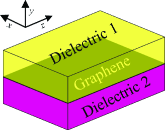
Figure 1: (Color Online) Schematic of the structure, where the graphene layer is placed on the $xz$ plane, and sandwiched by the dielectric 1 (yellow area) and dielectric 2 (pink area). The permittivities and permeabilities of the two dielectrics are ($\varepsilon_{1}$, $\mu_{1}$) and ($\varepsilon_{2}$, $\mu_{2}$), respectively.

This planar waveguide supports both the TM and TE plasmonic modes PRL99-016803 ; nanotechnology24-345203 , where the dispersion relation is

$$\frac{\varepsilon_{1}}{k_{1}}+\frac{\varepsilon_{2}}{k_{2}}+i\frac{\sigma_{g}}{\omega\varepsilon_{0}}=0$$ (1)

for the TM mode,

$$\frac{k_{1}}{\mu_{1}}+\frac{k_{2}}{\mu_{2}}-i\sigma_{g}\omega\mu_{0}=0$$ (2)

for the TE mode, $k_{1}=\sqrt{\beta^{2}-k_{0}^{2}\varepsilon_{1}\mu_{1}}$, $k_{2}=\sqrt{\beta^{2}-k_{0}^{2}\varepsilon_{2}\mu_{2}}$, $\omega=2\pi f$ is the angular frequency, $k_{0}=\omega/c$ is the wavenumber in free space, $\sigma_{g}$ is the surface conductivity of graphene, and $\beta$ is the propagation constant. If both the dielectric 1 and dielectric 2 are air, namely $\varepsilon_{1}=\varepsilon_{2}=1$ and $\mu_{1}=\mu_{2}=1$, the dispersion relation for the TM plasmonic mode reduces to

$$\beta=k_{0}\sqrt{1-\left(\frac{2}{\eta_{0}\sigma_{g}}\right)^{2}},$$ (3)

and the dispersion relation for the TE plasmonic mode reduces to

$$\beta=k_{0}\sqrt{1-\left(\frac{\eta_{0}\sigma_{g}}{2}\right)^{2}},$$ (4)

where $\eta_{0}=\sqrt{\mu_{0}/\varepsilon_{0}}$ is the characteristic impedance of free space.

Besides, the surface conductivity of monolayer graphene can be calculated according to the Kubo formula $\sigma_{g}\left(\omega,\mu_{c},\tau,T\right)=\sigma_{\text{intra}}+\sigma_{\text{inter}}$, where

$$\sigma_{\text{intra}}=\frac{ie^{2}k_{B}T}{\pi\hbar^{2}\left(\omega+i\tau^{-1}\right)}\left[\frac{\mu_{c}}{k_{B}T}+2\ln\left(e^{-\mu_{c}/k_{B}T}+1\right)\right]$$ (5)

is due to intraband contribution, and

$$\sigma_{\text{inter}}=\frac{ie^{2}\left(\omega+i\tau^{-1}\right)}{\pi\hbar^{2}}\int_{0}^{\infty}\frac{f_{d}\left(-\varepsilon\right)-f_{d}\left(\varepsilon\right)}{\left(\omega+i\tau^{-1}\right)^{2}-4\left(\varepsilon/\hbar\right)^{2}}d\varepsilon$$ (6)

is due to interband contribution JAP103-064302 ; JP19-026222 . In the above formula, $-e$ is the charge of an electron, $\hbar=h/2\pi$ is the reduced Plank’s constant, $T$ is the temperature, $\mu_{c}$ is the chemical potential, $\tau=\mu\mu_{c}/ev_{F}^{2}$ is the carrier relaxation time, $\mu$ is the carrier mobility which ranges from 1 000 $\text{cm}^{2}/(\text{V}\cdot\text{s})$ to 230 000 $\text{cm}^{2}/(\text{V}\cdot\text{s})$ ACSnano , $v_{F}=c/300$ is the Fermi velocity, $f_{d}\left(\varepsilon\right)=1/\left[e^{\left(\varepsilon-\mu_{c}\right)/k_{B}T}+1\right]$ is the Fermi-Dirac distribution, and $k_{B}$ is the Boltzmann’s constant. In the following, we choose a moderate mobility of $\mu=$ 50 000 $\text{cm}^{2}/(\text{V}\cdot\text{s})$, $T=300$ K, and the chemical potential $\mu_{c}$ is tuned between $0$ eV to $1$ eV JAP103-064302 . Due to the finite carrier relaxation time, the surface conductivity of graphene can be expressed as $\sigma_{g}=\sigma_{g,r}+i\sigma_{g,i}$, where the real part $\sigma_{g,r}$ is related to the optical loss of graphene, and the imaginary part $\sigma_{g,i}$ is related to the permittivity science332-1291 . Correspondingly, the propagation constant can also be expressed as $\beta=\beta_{r}+i\beta_{i}$ according to Eqs. (3)-(4), where the imaginary part $\beta_{i}$ is related to the propagation length of the plasmonic mode with $L=1/2\beta_{i}$ maier .

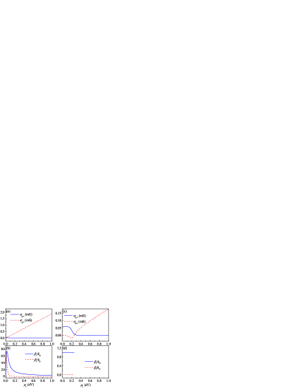
Figure 2: (Color Online) Top row: The dependence between the surface conductivity and the chemical potential, where $\sigma_{g,r}$ is the real part of surface conductivity, and $\sigma_{g,i}$ is the imaginary part. Bottom row: The dependence between the propagation constant and the chemical potential, where $\beta_{r}$ is the real part of propagation constant, and $\beta_{i}$ is the imaginary part. The incident frequency is $f=10$ THz for (a)-(b) and $f=100$ THz for (c)-(d).

Based on Eqs. (5)-(6), we can get the surface conductivity of monolayer graphene at different frequencies. As shown in Fig. 2(a), for $f=10$ THz, both the real and imaginary parts of surface conductivity are always positive. Since a positive $\sigma_{g,i}$ can lead to a negative permittivity, this implies that this structure supports the TM plasmonic mode, where the dependence between the propagation constant and the chemical potential is shown in Fig. 2 (b). From the imaginary part of surface conductivity, the propagation length of the TM plasmonic mode decreases for small chemical potentials. In contrast, the dependence between the surface conductivity and the chemical potential shows a different behavior for $f=100$ THz, as shown in Fig. 2(c). The imaginary part of surface conductivity is negative for $0$ eV $\leq\mu_{c}\leq 0.254$ eV, which implies the existence of the TE plasmonic mode. Fig. 2(d) shows the dependence between the propagation constant and the chemical potential of the TE mode, where the real part $\beta_{r}$ is nearly equal to the wavenumber in free space, and the imaginary part $\beta_{i}$ is nearly equal to zero. Thus the TE plasmonic mode supported by the planar waveguide is a weekly confined mode that can propagate for a long distance.

III Airy plasmons

In this section, we study the Airy plasmons that propagate in the planar plasmonic waveguide shown in Fig. 1. We assume that the solution of Airy plasmons is a perturbation of the plasmonic mode, and the Airy plasmons behave as a quasi-TM or quasi-TE mode approximately. The Helmholtz equation is

$$\nabla^{2}\Phi+k_{0}^{2}\varepsilon\left(y\right)\Phi=0,$$ (7)

where $\varepsilon\left(y\right)$ is the distribution of the relative permittivity, $\Phi=H_{y}(x,y,z)$ for the quasi-TM Airy plasmons, and $\Phi=E_{y}(x,y,z)$ for the quasi-TE Airy plasmons. The scalar field $\Phi\left(x,y,z\right)$ can be expressed as a functional dependence of the form

$$\Phi\left(x,y,z\right)=\psi\left(x,z\right)\Phi_{0}\left(y\right)\exp\left(i\beta z\right),$$ (8)

where the dimensionless scalar function $\psi\left(x,z\right)$ is dependent on both the transverse direction $x$ and the propagation direction $z$, the scalar function $\Phi_{0}\left(y\right)$ is only dependent on the transverse direction $y$, and $\beta$ is a parameter that is related to the $z$ component of the wavevector. Substituting Eq. (8) into Eq. (7), multiplying the result by $\Phi_{0}^{\ast}\left(y\right)$, and integrating over $y$ direction yields a scalar wave equation

$$\left[2i\beta\frac{\partial\psi}{\partial z}+\frac{\partial^{2}\psi}{\partial x^{2}}\right]+\left[\frac{I_{2}}{I_{0}}+k_{0}^{2}\varepsilon-\beta^{2}\right]\psi=0,$$ (9)

where $I_{0}=\int_{-\infty}^{+\infty}\left|\Phi_{0}\left(y\right)\right|^{2}dy$, $I_{2}=\int_{-\infty}^{+\infty}\Phi_{0}^{\prime\prime}\left(y\right)\Phi_{0}^{\ast}\left(y\right)dy$, and the term $\partial^{2}\psi/\partial z^{2}$ is neglected by employing the paraxial approximation OL35-2082 ; OL32-674 . For the slowly varying amplitude, the scalar function is expressed as $\psi\left(x,z\right)=\phi\left(x,z\right)\exp\left\{i\left[I_{2}/I_{0}+k_{0}^{2}\varepsilon\left(y\right)-\beta^{2}\right]/\left(2\beta\right)z\right\}$, which leads to the one-dimensional Schrödinger equation $i\phi_{z}\left(x,z\right)+\left(1/2\beta\right)\phi_{xx}\left(x,z\right)=0$. If the function $\Phi_{0}\left(y\right)$ is chosen as the magnetic (electric) field distribution of TM (TE) plasmonic mode of the waveguide, and the parameter $\beta=\beta_{r}+i\beta_{i}$ is the corresponding propagation constant, $I_{2}/I_{0}+k_{0}^{2}\varepsilon\left(y\right)-\beta^{2}=0$ and the Schrödinger equation for the amplitude $\psi$ is

$$i\frac{\partial\psi\left(s,\xi\right)}{\partial\xi}+\frac{\partial^{2}\psi\left(s,\xi\right)}{\partial s^{2}}=0,$$ (10)

where $s=x/x_{0}$ is the dimensionless transverse coordinate, $\xi=z/2\beta x_{0}^{2}$ is the dimensionless complex propagation distance, and $x_{0}$ is an arbitrary transverse scale.

For Eq. (10), its finite energy Airy plasmon solution at the input of $\psi\left(s,0\right)=\operatorname{Ai}\left(s\right)\exp\left(as\right)$ is

$$\psi\left(s,\xi\right)= \operatorname{Ai}\left(s-\xi^{2}+i2a\xi\right)\exp\left[i\left(s\xi+a^{2}\xi-2\xi^{3}/3\right)\right]$$

$$\times\exp\left(as-2a\xi^{2}\right),$$ (11)

where $a$ is a positive decay factor to truncate the amplitude at the negative infinity. According to the integral representation of Airy function Airy-function , Eq. (11) can also be built using plane waves

$$\psi\left(s,\xi\right)=\frac{1}{2\pi}\int_{-\infty}^{+\infty}\Phi\left(k_{s},\xi\right)e^{ik_{s}s}dk_{s},$$ (12)

where

$$\Phi\left(k_{s},\xi\right)=e^{\frac{a^{3}}{3}}e^{-ia^{2}k_{s}}e^{-ak_{s}^{2}}e^{i\frac{k_{s}^{3}}{3}}e^{-ik_{s}^{2}\xi}$$ (13)

is the Fourier spectrum of the $k$-space, the cubic phase term $\exp\left(ik_{s}^{3}/3\right)$ is associated with the spectrum of the Airy wave, the first Gaussian function $\exp\left(-ak_{s}^{2}\right)$ arises from the exponential apodization of the beam, and the second Gaussian function $\exp\left(k_{s}^{2}\xi_{i}\right)$ is nonzero with $\xi_{i}=-\beta_{i}z/\left[2\left(\beta_{r}^{2}+\beta_{i}^{2}\right)x_{0}^{2}\right]$ because of the optical loss of graphene. From Eqs. (8), (12)-(13), the $x$ and $z$ components of the wavevector are $k_{x}=k_{s}/x_{0}$ and $k_{z}=\left(\beta_{r}+\delta\beta_{r}\right)+i\left(\beta_{i}+\delta\beta_{i}\right)$, respectively, where $\delta\beta_{r}=-k_{x}^{2}\beta_{r}/\left[2\left(\beta_{r}^{2}+\beta_{i}^{2}\right)\right]$, and $\delta\beta_{i}=k_{x}^{2}\beta_{i}/\left[2\left(\beta_{r}^{2}+\beta_{i}^{2}\right)\right]$. To insure the validity of the quasi-TM or quasi-TE mode condition, the wavevector components must satisfy $\left|k_{x}\right|\ll\beta_{r}$, $\left|\delta\beta_{r}\right|\ll\beta_{r}$, and $\left|\delta\beta_{i}\right|\ll\beta_{i}$. Given the Gaussian spectrum of the Airy plasmon in Eq. (13), the three conditions reduce to

$$\sqrt{a+\frac{\beta_{i}z}{2\left(\beta_{r}^{2}+\beta_{i}^{2}\right)x_{0}^{2}}}\beta_{r}x_{0}\gg 1.$$ (14)

Since Eq. (14) should be fulfilled for arbitrary propagation distance $z$, we let

$$\sqrt{a}\beta_{r}x_{0}\gg 1.$$ (15)

Besides, the paraxial approximation holds provided that $\left|\partial^{2}\psi/\partial z^{2}\right|\ll\left|2i\beta\partial\psi/\partial z\right|$, namely $\left|\delta\beta\right|\ll 2\left|\beta\right|$. This approximation also holds, if Eq. (15) is valid.

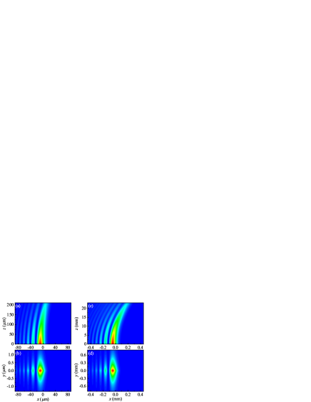
Figure 3: (Color Online) Left panel: The magnetic field intensity distribution of the quasi-TM Airy plasmons at (a) the $xz$ plane with $y=0$ and (b) the $xy$ plane with $z=0$, respectively, where $a=0.1$, $f=10$ THz, $x_{0}=10$ $\mu$m, and $\mu_{c}=0.8$ eV. Right panel: The electric field intensity distribution of the quasi-TE Airy plasmons at (c) the $xz$ plane with $y=0$ and (d) the $xy$ plane with $z=0$, respectively, where $a=0.1$, $f=100$ THz, $x_{0}=50$ $\mu$m, and $\mu_{c}=0.1$ eV.

Considering the optical loss of graphene and according to Eq. (11), the parabolic self-deflection experienced by the Airy plasmons during propagation can be estimated as

$$z^{2}=4\beta_{r}^{2}x_{0}^{3}x.$$ (16)

Taking $L_{a}=1/2\beta_{i}$ as the analytically estimated propagation length of Airy plasmons OL35-2082 , the transverse displacement of the beam at the propagation length can be calculated analytically as

$$\Delta x_{a}(z=L_{a})=\frac{1}{16\beta_{r}^{2}\beta_{i}^{2}x_{0}^{3}}.$$ (17)

To realized the Airy plasmons in graphene-based waveguides, Eq. (15) must be fulfilled to insure the validity of the paraxial approximation. Since the decay factor $a$ is usually small to avoid excessively changing the non-diffracting behavior of Airy beams, the real part of propagation constant $\beta_{r}$ and the transverse scale $x_{0}$ must be large enough. However, from Eq. (17), the decrease of the transverse displacement $\Delta x_{a}$ would be a challenge for the detection and measurement of Airy plasmons experimentally. A contradiction exists between the validity of the paraxial approximation and a large enough transverse displacement.

From Eq. (11), the decay factor $a$ imposes an attenuation to the propagation of Airy plasmons, and $\xi_{i}$ introduces extra exponential terms. This imposes errors to the analytical results $L_{a}$ and $\Delta x_{a}$. Thus we can also calculate the propagation length of Airy plasmons numerically, and compare it with $L_{a}$. The propagation length $L_{n}$ is defined as the distance where the input power $P=\int_{-\infty}^{+\infty}\left|\Phi\left(x,y=0,z\right)\right|^{2}dx$ decreases to $e^{-1}P_{0}$ along the propagation direction, where $P_{0}=\int_{-\infty}^{+\infty}\left|\Phi\left(x,y=0,z=0\right)\right|^{2}dx$ is the initial input power. Accordingly, the transverse displacement $\Delta x_{n}$ can be defined as the displacement of the maximum field intensity during propagation. Since the solution of Airy plasmons is assumed to be a perturbation of the plasmonic mode, our model is valid if the analytical propagation length $L_{a}$ and transverse displacement $\Delta x_{a}$ are approximately equal to the numerical propagation length $L_{n}$ and transverse displacement $\Delta x_{n}$, respectively.

First, we focus on the quasi-TM Airy plasmons. Figs. 3(a) and (b) show the magnetic field intensity distributions at the $xz$ plane with $y=0$ and the $xy$ plane with $z=0$, respectively, where the parameters are $a=0.1$, $f=10$ THz, $x_{0}=10$ $\mu$m, and $\mu_{c}=0.8$ eV to insure the validity of Eq. (15). The field intensity at the $xz$ plane exhibits the self-deflection behavior of Airy beam, and the intensity at the $xy$ plane is governed by the localized TM plasmonic mode of the graphene-based waveguide. Since the TM mode is highly localized along the graphene surface, the width of the main lobe is much larger than its height. Meanwhile, although the surface conductivity of monolayer graphene is almost purely imaginary with $\sigma_{g}=0.006+1.498i$ mS, the energy attenuation experienced by TM Airy plasmons is large and the propagation length is quite limited. For the parameters in Figs. 3(a) and (b), the propagation length is $L_{n}=170.5$ $\mu$m ($L_{a}=175.4$ $\mu$m), and the corresponding transverse displacement at the propagation length is $\Delta x_{n}=12.1$ $\mu$m ($\Delta x_{a}=12.9$ $\mu$m), where the analytical result is nearly equal to the numerical result. If we take $2x_{0}$ as a measure of the width of the main lobe, the beam is only displaced by half width approximately.

Similarly, for the quasi-TE Airy plasmons, Figs. 3(c) and (d) show the electric field intensity distribution at the $xz$ plane with $y=0$ and $xy$ plane with $z=0$, respectively, where the parameters are $a=0.1$, $f=100$ THz, $x_{0}=50$ $\mu$m, and $\mu_{c}=0.1$ eV to insure the validity of Eq. (15). The field intensity at the $xz$ plane also exhibits the self-deflection behavior of Airy beam, while the intensity at the $xy$ plane is governed by the localized TE plasmonic mode of graphene-based waveguide. Since the TE mode is weakly localized along the graphene surface, the width of the main lobe is much smaller than its height. Meanwhile, the energy attenuation experienced by TE Airy plasmons is small, and the propagation length is quite large due to the weak localized field. For the parameters in Figs. 3(c) and (d), the propagation length is $L_{n}=28.1$ mm ($L_{a}=29.6$ mm), and the corresponding transverse displacement at the propagation length is $\Delta x_{n}=0.4$ mm ($\Delta x_{a}=0.4$ mm), which is about 4 times of the width of the main lobe.

By comparing the quasi-TM Airy plasmons with the quasi-TE Airy plasmons, we can conclude that the quasi-TE Airy plasmons have a larger transverse displacement because of the weak confinement and low propagation loss. This is favourable to the realization of Airy beams in experiments. However, as shown in Fig. 2, the propagation constant of TM plasmonic mode is sensitive to the chemical potential of graphene, which can be tuned by the chemical doping and/or a gate voltage JAP103-064302 . Thus the propagation of TM Airy plasmons can be steered by the chemical potential externally.

IV Beam steering

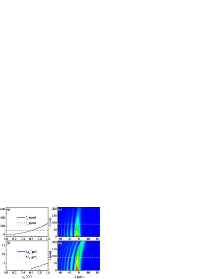
Figure 4: (Color Online) Left panel: (a)-(b) The (a) propagation length and (b) transverse displacement at $z=90$ $\mu$m of quasi-TM Airy plasmons in the monolayer graphene based waveguide for different values of chemical potential, where $L_{n}$ and $\Delta x_{n}$ are numerical results, and $L_{a}$ and $\Delta x_{a}$ are analytical results. Right panel: The magnetic field intensity distributions of the quasi-TM Airy plasmons at the $xz$ plane with $y=0$ for (c) $\mu_{c}=0.6$ eV, and (d) $1.0$ eV, respectively. The dashed black line in (a) and white lines in (c)-(d) indicate $z=90$ $\mu$m. The parameters are $a=0.1$, $f=10$ THz, and $x_{0}=10$ $\mu$m.

To steer the self-deflection behavior of quasi-TM Airy plasmons, the chemical potential of monolayer graphene can be tuned externally. As shown in Fig. 4 (a), the propagation length of Airy plasmons changes effectively when the chemical potential changes, where the parameters are $a=0.1$, $f=10$ THz, and $x_{0}=10$ $\mu$m to insure the validity of Eq. (15). Note the analytical result $L_{a}$ calculated from Eq. (16) agrees well with the numerical result $L_{n}$. When the chemical potential is small, the imaginary part of the propagation constant $\beta_{i}$ is large and the corresponding propagation length is small. This is unfavorable for the propagation of Airy plasmons.

To evaluate the tunability of self-deflection behavior, we require that the propagation length should be larger than $90$ $\mu$m, which is 3 times of the wavelength in free space. Under this requirement, the chemical potential is within $0.6$ eV $\leq\mu_{c}\leq 1.0$ eV, and the transverse displacement of Airy plasmons at $z=90$ $\mu$m varies from $2.0$ $\mu$m to $5.1$ $\mu$m, as shown in Fig. 4(b). Fig. 4 (c)-(d) show the magnetic field intensity distribution of the quasi-TM Airy plasmons in the monolayer graphene based waveguide for $\mu_{c}=0.6$ eV, and $1.0$ eV, respectively. Clearly, the transverse displacement is changed effectively, which is promising for the detection, sensing, and other applications.

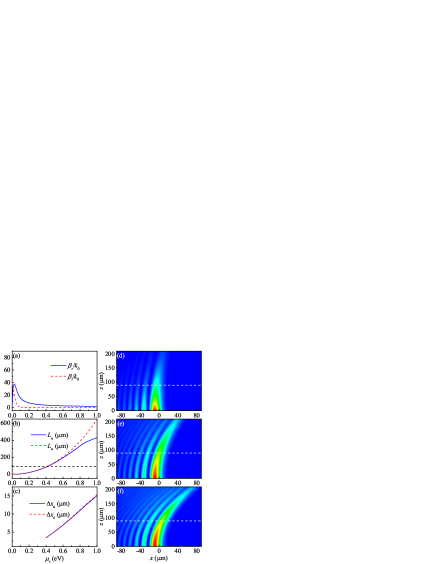
Figure 5: (Color Online) Left panel: (a) The dependence between the propagation constant and the chemical potential for the TM plasmonic mode in the bilayer graphene based waveguide, where $\beta_{r}$ is the real part of propagation constant, and $\beta_{i}$ is the imaginary part. (b)-(c) The (b) propagation length and (c) transverse displacement at $z=90$ $\mu$m of quasi-TM Airy plasmons for different values of the chemical potential, where $L_{n}$ and $\Delta x_{n}$ are numerical results, and $L_{a}$ and $\Delta x_{a}$ are analytical results. Right panel: The magnetic field intensity distributions of the quasi-TM Airy plasmons at the $xz$ plane with $y=0$ for (d) $\mu_{c}=0.4$ eV, (e) $0.7$ eV, and (f) $1.0$ eV, respectively. The dashed black line in (b) and white lines in (d)-(f) indicate $z=90$ $\mu$m. The parameters are $a=0.1$, $f=10$ THz, and $x_{0}=10$ $\mu$m.

In the above discussion, we always use monolayer graphene. However, multilayer graphene is also important for the study of Airy plasmons. First, it is hard to fabricate the strict monolayer graphene in experiments, and it is very likely that the used graphene is not monolayer in practical applications. Second, the plasmonic mode supported by the multilayer graphene has a longer propagation length APL101-111609 ; JLT32-3597 , and it is likely to increase the propagation length and transverse displacement of Airy plasmons by increasing the number of layers of graphene. Considering the two factors, in the following, we study the Airy plasmons and try to improve the tunability of beam steering based on multilayer graphene.

The surface conductivity of multilayer graphene can be calculated as $N\sigma_{g}$ for $N<6$ LPR8-291 ; NL7-2711 ; nnano7-330 , where $N$ is the number of layers, and $\sigma_{g}$ is the surface conductivity of monolayer graphene. For the calculation of plasmonic mode and Airy plasmons based on multilayer graphene, we only need to replace $\sigma_{g}$ for the monolayer graphene with $N\sigma_{g}$. We consider the bilayer graphene with $N=2$ as an example. As shown in Fig. 5 (a), both the real and imaginary parts of propagation constant of TM plasmonic mode in the bilayer graphene based waveguide decrease compared with the results shown in Fig. 2(b). Thus, for the same parameters of $a=0.1$, $f=10$ THz, and $x_{0}=10$ $\mu$m, Airy plasmons based on bilayer graphene have a larger propagation length, as shown in Fig. 5 (b). Meanwhile, the transverse displacement at a same propagation distance would also increase according to Eq. (16). Note in Fig. 5 (b), the analytical results deviate from the numerical results for large values of chemical potential. This is due to the decrease of $\sqrt{a}\beta_{r}x_{0}$ in the paraxial approximation condition of Eq. (15).

Similarly, to evaluate the tunability of self-deflection behavior, we also require that the propagation length should be larger than $90$ $\mu$m. Under this requirement, the chemical potential of bilayer graphene is within $0.4$ eV $\leq\mu_{c}\leq 1.0$ eV, and the transverse displacement of Airy plasmons at $z=90$ $\mu$m varies from $3.4$ $\mu$m to $15.2$ $\mu$m. The range of transverse displacement is almost 4 times of that for the Airy plasmons based on monolayer graphene. Fig. 5 (d)-(f) show the magnetic field intensity distribution of the quasi-TM Airy plasmons in the bilayer graphene based waveguide for $\mu_{c}=0.4$ eV, $0.7$ eV, and $1.0$ eV, respectively. Compared with the Airy plasmons based on monolayer graphene, Airy plasmons based on bilayer graphene shows a larger tunability, where the self-deflection behavior can be tuned more effectively. Thus the multilayer graphene provides a better platform to the beam steering compared with the monolayer graphene.

V Conclusion

In conclusion, we derive an analytical model under the paraxial approximation to study the Airy plasmons in graphene-based waveguides. Both the quasi-transverse-magnetic (TM) and quasi-transverse-electric (TE) Airy plasmons can be supported, where the quasi-TE Airy plasmons have larger propagation length and transverse displacement, and the quasi-TM Airy plasmons show a better tunability to steer the self-deflection behavior. Moreover, for the quasi-TM Airy plasmons, the propagation length and the range of transverse displacement can be increased, if multilayer graphene is used in the graphene-based waveguides. Besides the metals, graphene provides an additional platform to investigate the propagation of Airy plasmons and to design various plasmonic devices.

VI Acknowledgment

This work was sponsored by the National Natural Science Foundation of China under Grants No. 61322501, No. 61574127, and No. 61275183, the Top-Notch Young Talents Program of China, the Program for New Century Excellent Talents (NCET-12-0489) in University, the Fundamental Research Funds for the Central Universities, and the Innovation Joint Research Center for Cyber-Physical-Society System.

References

- (1) D. Dragoman, and M. Dragomann, Quantum-Classical Analogies (Springer, Berlin, 2004).
- (2) S. Longhi, Quantum-optical analogies using photonic structures, Laser Photonics Rev. 3, 243 (2009).
- (3) M. V. Berry, and N. L. Balazs, Nonspreading wave packets, Am. J. Phys. 47, 264 (1979)
- (4) G. A. Siviloglou, and D. N. Christodoulides, Accelerating finite energy Airy beams, Opt. Lett. 32, 979 (2007).
- (5) I. M. Besieris, and A. M. Shaarawi, A note on an accelerating finite energy Airy beam, Opt. Lett. 32, 2447 (2007).
- (6) G. A. Siviloglou, J. Broky, A. Dogariu, and D. N. Christodoulides, Observation of Accelerating Airy Beams, Phys. Rev. Lett. 99, 213901 (2007).
- (7) J. Broky, G. A. Siviloglou, A. Dogariu, and D. N. Christodoulides, Self-healing properties of optical Airy beams, Opt. Exp. 16, 12880 (2008).
- (8) A. Chong, W. H. Renninger, D. N. Christodoulides, and F. W. Wise, Airy-Bessel wave packets as versatile linear light bullets, Nat. Photon. 4, 103 (2010).
- (9) K.-Y. Kim, C.-Y. Hwang, and B. Lee, Slow non-dispersing wavepackets, Opt. Exp. 19, 2286 (2011).
- (10) T. Schneider, A. A. Serga, A. V. Chumak, C. W. Sandweg, S. Trudel, S. Wolff, M. P. Kostylev, V. S. Tiberkevich, A. N. Slavin, and B. Hillebrands, Nondiffractive Subwavelength Wave Beams in a Medium with Externally Controlled Anisotropy, Phys. Rev. Lett. 104, 197203 (2010).
- (11) P. Polynkin, M. Kolesik, J. V. Moloney, G. A. Siviloglou, D. N. Christodoulides, Curved Plasma Channel Generation Using Ultraintense Airy Beams, Science 324, 229 (2009).
- (12) S. Fu, Y. Tsur, J. Zhou, L. Shemer, and A. Arie, Propagation Dynamics of Airy Water-Wave Pulses, Phys. Rev. Lett. 115, 034501 (2015).
- (13) A. E. Minovich, A. E. Klein, D. N. Neshev, T. Pertsch, Y. S. Kivshar, and D. N. Christodoulides, Airy plasmons: non-diffracting optical surface waves, Laser Photon. Rev. 8, 221 (2014).
- (14) A. Salandrino, and D. N. Christodoulides, Airy plasmon: a nondiffracting surface wave, Opt. Lett. 35, 2082 (2010).
- (15) A. Minovich, A. E. Klein, N. Janunts, T. Pertsch, D. N. Neshev, and Y. S. Kivshar, Generation and Near-Field Imaging of Airy Surface Plasmons, Phys. Rev. Lett. 107, 116802 (2011).
- (16) P. Zhang, S. Wang, Y. Liu, X. Yin, C. Lu, Z. Chen, and X. Zhang, Plasmonic Airy beams with dynamically controlled trajectories, Opt. Lett. 36, 3191 (2011).
- (17) L. Li, T. Li, S. M. Wang, C. Zhang, and S. N. Zhu, Plasmonic Airy Beam Generated by In-Plane Diffraction, Phys. Rev. Lett. 107, 126804 (2011).
- (18) A. E. Klein, A. Minovich, M. Steinert, N. Janunts, A. Tünnermann, D. N. Neshev, Y. S. Kivshar, and T. Pertsch, Controlling plasmonic hot spots by interfering Airy beams, Opt. Lett. 37, 3402 (2012).
- (19) W. Liu, D. N. Neshev, I. V. Shadrivov, A. E. Miroshnichenko, and Y. S. Kivshar, Plasmonic Airy beam manipulation in linear optical potentials, Opt. Lett. 36, 1164 (2011).
- (20) F. Bleckmann, A. Minovich, J. Frohnhaus, D. N. Neshev, and S. Linden, Manipulation of Airy surface plasmon beams, Opt. Lett. 38, 1443 (2013).
- (21) F. H. L. Koppens, D. E. Chang, and F. J. Garcsia de Abajo, Graphene Plasmonics: A Platform for Strong Light-Matter Interactions, Nano Lett. 11, 3370 (2011).
- (22) A. H. C. Neto, F. Guinea, N. M. R. Peres, K. S. Novoselov, and A. K. Geim, The electronic properties of graphene, Rev. Mod. Phys. 81, 109 (2009).
- (23) N. M. R. Peres, Colloquium: The transport properties of graphene: An introduction, Rev. Mod. Phys. 82, 2673 (2010).
- (24) S. D. Sarma, S. Adam, E. H. Hwang, and E. Rossi, Electronic transport in two-dimensional graphene, Rev. Mod. Phys. 83, 407 (2011).
- (25) A. Vakil, and N. Engheta, Transformation Optics Using Graphene, Science 332, 1291 (2011).
- (26) Y. Yang, H. T. Dai, B. F. Zhu, and X. W. Sun, Dynamic Control of the Airy Plasmons in a Graphene Platform, IEEE Photonics J. 6, 4801207 (2014).
- (27) S. A. Mikhailov, and K. Ziegler, New Electromagnetic Mode in Graphene, Phys. Rev. Lett. 99, 016803 (2007).
- (28) X. He, J. Tao, and B. Meng, Analysis of graphene TE surface plasmons in the terahertz regime, Nanotechnology 24, 345203 (2013).
- (29) G. W. Hanson, Dyadic Green’s functions and guided surface waves for a surface conductivity model of graphene, J. Appl. Phys. 103, 064302 (2008).
- (30) V. P. Gusynin, S. G. Sharapov, and J. P. Carbotte, Magneto-optical conductivity in graphene, J. Phys. 19, 026222 (2007).
- (31) W. Gao, J. Shu, C. Qiu, and Q. Xu, Excitation of Plasmonic Waves in Graphene by Guided-Mode Resonances, ACS Nano 6, 7806 (2012).
- (32) S. A. Maier, Plasmonics: Fundamentals and applications (Springer, New York, 2007).
- (33) E. Feigenbaum, and M. Orenstein, Plasmon-soliton, Opt. Lett. 32, 674 (2007).
- (34) M. Abramowitz, and I. A. Stegun, Handbook of Mathematical Functions (Dover, 1972).
- (35) C. H. Gan, Analysis of surface plasmon excitation at terahertz frequencies with highly doped graphene sheets via attenuated total reflection, Appl. Phys. Lett. 101, 111609 (2012).
- (36) X. Zhou, T. Zhang, L. Chen, W. Hong, and X. Li, A Graphene-Based Hybrid Plasmonic Waveguide With Ultra-Deep Subwavelength Confinement, J. Lighwave Techno. 32, 3597 (2014).
- (37) D. A. Smirnova, I. V. Shadrivov, A. I. Smirnov, and Y. S. Kivshar, Dissipative plasmon-solitons in multilayer graphene, Laser Photonics Rev. 8, 291 (2013).
- (38) C. Casiraghi, A. Hartschuh, E. Lidorikis, H. Qian, H. Harutyunyan, T. Gokus, K. S. Novoselov, and A. C. Ferrari, Rayleigh Imaging of Graphene and Graphene Layers, Nano Lett. 7, 2711 (2007).
- (39) H. Yan, X. Li, B. Chandra, G. Tulevski, Y. Wu, M. Freitag, W. Zhu, P. Avouris, and F. Xia, Tunable infrared plasmonic devices using graphene/insulator stacks, Nature Nanotech. 7, 330 (2012).