Buoyancy-driven inflow to a relic cold core: the gas belt in radio galaxy 3C 386

Abstract

We report measurements from an XMM-Newton observation of the low-excitation radio galaxy 3C 386. The study focusses on an X-ray-emitting gas belt, which lies between and orthogonal to the radio lobes of 3C 386 and has a mean temperature of $0.94\pm 0.05$ keV, cooler than the extended group atmosphere. The gas in the belt shows temperature structure with material closer to the surrounding medium being hotter than gas closer to the host galaxy. We suggest that this gas belt involves a ‘buoyancy-driven inflow’ of part of the group-gas atmosphere where the buoyant rise of the radio lobes through the ambient medium has directed an inflow towards the relic cold core of the group. Inverse-Compton emission from the radio lobes is detected at a level consistent with a slight suppression of the magnetic field below the equipartition value.

1 Introduction

Radio galaxies fuelled by active galactic nuclei (AGN) inject energy into the surrounding medium and are important sources of heating in galaxy groups and clusters (Scheuer, 1974). Energy transfer via an AGN feedback process is inferred most directly through gas cavities created by jet structures, which are seen frequently at the centres of clusters in the local Universe (McNamara & Nulsen, 2007). Cavities are formed when a radio jet does work on gas, pushing it away from the densest regions of the group or cluster environment. Along with cavities, many galaxies in group environments display prominent belt-like gas structures, which are associated with the central narrowing of radio sources between their radio lobes (Mannering et al., 2013; Mannering, 2013).

Belted sources such as 3C 35, 3C 285 and 3C 442A have previously been studied, with different conclusions as to their origins. For 3C 35, Mannering et al. (2013) interpret the gas belt as fossil-group gas driven outwards by the expanding radio lobes. Hardcastle et al. (2007) refer to the thermal gas which is aligned orthogonal to the radio lobes in 3C 285 as a ridge. They suggest the ridge was present long before radio activity commenced, and only a small fraction of the gas was contributed by merger activity involving 3C 285’s host galaxy. In the case of 3C 442A, Worrall et al. (2007) conclude that an active merger is causing the gas of merging galaxies to align orthogonal to, and do work on, the radio lobes.

For the three belted sources studied previously in detail, the gas appears to be either relatively stagnant or to be flowing away from the host galaxy. This could cause a barrier to positive feedback which requires AGN activity and black hole growth to be linked to gas-cooling and star formation, although the mechanisms may assist a negative feedback cycle. Alternatively, it is possible that some belts could result from gas driven inwards towards the AGN. This could potentially cause runaway positive feedback, if gas cooling from the outer atmosphere can reach the pc-scale regions around the central black hole, and provide extra fuel to renew or prolong AGN activity. In this paper, we add a fourth source, 3C 386, to the detailed study of belted sources, using new data from XMM-Newton. We present evidence that 3C 386 does indeed exhibit behaviour that is opposite to that seen in the previously studied cases.

1.1 3C 386

3C 386 is a low-excitation radio galaxy with an elliptical host which lies around 75 Mpc ($z$=0.0177) away. It is a ‘fat’ or ‘relaxed double’ radio galaxy, and provides an example where the absence of jets and hot spots (Strom et al., 1978) probably indicates little current relativistic particle acceleration (Young et al., 2005). It is a fairly typical relaxed double source, with its lobes containing fine structure including filaments near the edges which may form shells (Leahy & Perley, 1991). It is roughly 210″ $\times$ 290″ in angular size, which corresponds to projected dimensions of 76 kpc $\times$ 105 kpc in the source rest frame. The central region of the host galaxy of 3C 386 appears bright in the optical due to the chance superposition of an F7 type Galactic star (Lynds, 1971; Buttiglione et al., 2009). There are several other optical point sources discernible within a radius of about 30 kpc; some of which may be globular clusters (Madrid et al., 2006).

3C 386’s environment is classified as isolated: only two L^∗ galaxies are seen within an 800$h_{75}^{-1}$ kpc radius compared to an expected 0.9 field galaxies (Miller et al., 1999). Mannering (2013) examined 3C 386’s environment using Spitzer data taken with the Infrared Array Camera (IRAC) and found 13 faint, but plausibly associated galaxies within a 0.5 Mpc radius. Additionally, there are two galaxies with velocities within 500 km s^-1 of 3C 386’s velocity (Miller et al., 2002). A galaxy close in projected distance is two magnitudes fainter than 3C 386’s host at 3.6 $\mu$m. Mannering (2013) confirms the isolated environmental classification, as potential companions are too small to contribute significant gas and/or too distant to cause major disturbances in 3C 386’s gas belt.

Non-detections of 3C 386 in the X-ray were reported for both Einstein and ROSAT (Feigelson & Berg, 1983; Miller et al., 1999), but it was subsequently detected with Chandra (Ogle et al., 2010; Mannering, 2013). While Ogle et al. (2010) studied the nucleus, Mannering (2013) investigated several X-ray components associated with 3C 386. Using a 30 ks Chandra observation (Obs ID 10232), a rectangular region defining the gas belt indicated a temperature of $kT\approx 1.1$ keV. Ineson et al. (2015) fitted a single component radial profile through the belt and beyond and spectrally fitted all emission in an annulus of radii 2.46″to 270″to $kT=1.05^{+0.18}_{-0.12}$. Mannering (2013) suggests that the gas belt is consistent with a hot gas halo surrounding an isolated field elliptical. She finds the belt to be overpressured relative to the surrounding environment by up to an order of magnitude, and notes that its asymmetric morphology suggests an interaction with the radio source in the past. She, however, comes to no conclusion regarding the origins of the gas in the belt.

We use a new 92 ks XMM-Newton observation to investigate the gas belt in 3C 386. In Section 2, the observation and the process of data reduction are described. In Sections 3 and 4 the X-ray morphology of 3C 386, and the results of the spectral fitting are discussed. Throughout this paper a flat $\Lambda$CDM cosmology with $\Omega_{m0}=0.3$ and $\Omega_{\Lambda 0}=0.7$ is adopted, with $H_{0}=70$ km s^-1 Mpc^-1.

2 XMM-Newton Observation and Data Reduction

3C 386 was observed with XMM-Newton for 92 ks on 11-12 September 2013. Data presented here are from the EPIC MOS1, MOS2 and pn cameras in full-frame mode. The Observation Data Format (ODF) files were reprocessed using the tasks emchain for the MOS detectors and epchain for the pn detector. We make use of the XMM-Newton Extended Source Analysis Software procedure (XMM-ESAS) along with the relevant current calibration files (CCF) which contain filter wheel closed (FWC), quiescent particle background (QPB) and soft proton (SP) calibration data.

Due to the high variability of solar flares, the SP component of the observation cannot be well removed using background subtraction. Instead, frames which are dominated by high flare count rates must be excluded, reducing the net exposure time. We created a Good Time Intervals (GTI) file for using the XMM-ESAS tasks mos-filter and pn-filter to generate SP contamination-filtered products for the field of view data. The energy range used in determining the GTI for both the MOS and PN detectors was 2.5-12 keV. From the generated light curves, it was clear that only a small part of the observation was dominated by high flaring. Net exposure times for each detector are listed in Table 1.

Detector	Duration (ks)	Net exposure (ks)
MOS1	90.7	73.3
MOS2	90.6	73.8
pn	88.1	60.7

Table 1: XMM-Newton exposure times. The duration refers to the total observation time, whereas the net exposure is the time remaining after the high flare-count-rate frames have been excluded.

For the MOS1 detector, CCD 3 and CCD 6 were excluded from subsequent processing, as both had previously suffered from micrometeorite damage. In the same strike which damaged CCD 3, CCD 4 sustained collateral damage causing low energy events to dominate towards the high $x$ values in detector coordinates (DETX). To avoid entirely excluding CCD 4 from subsequent analysis, we created a histogram of the number of events as a function of the $x$ position in DETX, to determine a cutoff for good data (in this instance DETX $\approx$ 9750), and included this in later spectral analysis (Snowden & Kuntz, 2011).

We used the XMM-ESAS task cheese, which runs source detection on full-field images and then outputs a mask image of these sources for use in creating source-excluded spectra. It was noted that a few compact sources apparent by eye were not detected by the cheese task, so we modified the mask to exclude them too. Following this, the tasks mos-spectra and pn-spectra were run. These extract spectra from the cleaned event files for a selected region. Finally, the XMM-ESAS processes mos$\_$back and pn$\_$back were utilised to create particle background spectra for the relevant regions. The XMM-Newton background was sampled away from the source and fitted to models using methods described in Section 4.1. Spectra were binned using a minimum of 25 counts per bin, over a range of 0.4-8.5 keV for the MOS detectors and 0.4-7.2 keV for the pn detector. A Galactic absorption of $N_{\rm H}=1.81\times 10^{21}$ cm^-2 was applied to all spectral components described as ‘absorbed’.

3 X-ray Morphology

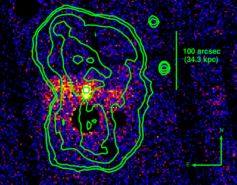
Figure 1: Particle background subtracted and exposure corrected MOS and pn combined XMM-Newton image between 0.4 and 8.5 keV with 2.5″ pixels. Point sources excluding the AGN nucleus have been excised from the image. Contours are of a 1.4 GHz VLA map 0.2, 1, 5, 10, 15 mJy/beam (5.8″  beam). The radio map is taken from Leahy & Perley (1991).

Figure 1 shows an image of the MOS1, MOS2 and pn data combined using the task comb, which adds the counts from the three instruments, accounting for differing exposures. The image in Figure 1 was background subtracted, to remove the SP and QPB components. Point sources unrelated to the source are excised. Across the centre of the radio source, between the north and south lobes, there is a clear excess of X-ray emission which we describe as the gas belt. The brightening in the centre of this belt corresponds to a superposition of the AGN core and the Galactic F7 star. The slight misalignment between these produces the elliptical shape of the core seen in Figure 1. The gas belt extends about 145″, which corresponds to a projected length of 53 kpc in the source rest frame.

A polygonal region for the spectral extraction across the belt was defined by eye (see Figure 2). The core was not included in the spectral extraction for the belt.

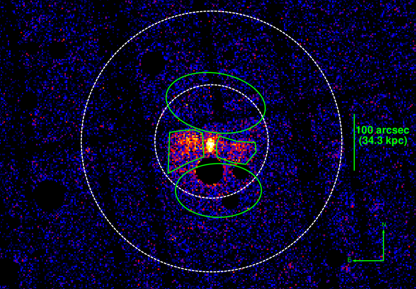
Figure 2: Image of 3C 386 with native 2.5″ pixels, with green regions highlighting the extraction region for the gas belt and the north and south lobes and the dashed white region highlighting the extraction region for the extended group emission.

4 Spectroscopy

4.1 Background Estimation

We reduced the flare-free XMM-Newton data using the XMM-ESAS software package. For our primary analysis we chose to model the background, using local background subtraction to check for consistency. The model background used spectra extracted from a circular off-source region, away from the source and its associated gas belt and group gas. The location of the extraction region differs between detectors in order to avoid chip gaps, but for each it is extracted from an area of blank sky. The local background region was extracted from an annulus surrounding 3C 386.

The modelled background is preferred to subtracting a local background as it can accommodate variation in background counts across the field of view. Due to this, unless explicitly stated, values quoted in this paper will be those measured from fits with modelled background. The local background is simply used as a method of cross checking.

We follow the prescription of Mannering et al. (2013), who in turn followed Snowden & Kuntz (2011), to model the XMM-Newton background component. The XMM-Newton tasks mos$\_$back and pn$\_$back generate model QPB spectra from the FWC observations and unexposed corners of the MOS and pn CCDs, respectively. This quiescent instrumental background is subtracted from data, and then additional components in the XMM-Newton background need to be modelled explicitly. Instrumental Al K$\alpha$ and Si K$\alpha$ lines were fitted with unabsorbed Gaussians of zero intrinsic widths at line energies of 1.49 keV and 1.75 keV, respectively, for the MOS detectors, whilst only the Al K$\alpha$ line at 1.49 keV was required for the pn data. The energy range for the pn detector was restricted between 0.4 and 7.2 keV, due to the difficulty in modelling the QPB at high energies for this detector and the large number of instrumental Cu K$\alpha$ lines present at 7.49 keV and above.

The cosmic X-ray background was modelled by an unabsorbed thermal component representing emission from the heliosphere at $kT\approx 0.1$ keV, a higher temperature ($kT\approx 0.25-0.7$ keV) absorbed thermal component representing emission from the hotter halo and intergalactic medium, and an absorbed power law with $\Gamma\approx 1.46$ representing the unresolved background of cosmological sources. We also included a cool, ($kT\approx 0.1$ keV) absorbed thermal component representing emission from the cooler halo, but this was fit with a very small normalisation and was unnecessary. In order to further constrain the cosmic background contribution, a ROSAT All Sky Survey (RASS) spectrum from the HEASARC X-ray Background Tool was also included.

Solar Wind Charge Exchange (SWCX) emission, which originates in the heliosphere, contributes a significant fraction of the X-ray background at energies of less than 1 keV. The ions of high charge state in the solar wind interact with neutral atoms, thereby gaining an electron in a highly excited state. This electron decays by emitting X-rays, which produces a background strongly dependent on the solar wind proton flux and heavy ion abundances. We included several SWCX lines in our XMM-Newton background model, represented by additional Gaussians at several line energies with zero intrinsic width. These were identified by fitting a model containing the instrumental Gaussian and cosmic X-ray background components, and adding the SWCX at relevant energies to improve the fit.

Data and responses for the three XMM detectors were not combined before spectral fitting. Rather, their data were fitted concurrently to the same models. Between each data set several parameters are held common; these include the energies and widths of each Gaussian used to describe a line, and parameters such as the redshift of the source and the abundances and temperatures of each part of the cosmic X-ray background model. The best-fit model for the off-source data (Fig. 3) has $\chi^{2}=$ 600.4 for 621 degrees of freedom.

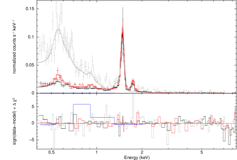
Figure 3: XMM-Newton spectra extracted from the off-source region, and fit to the background model described in Section 4.1. Black, red, and grey correspond to MOS1, MOS2, and pn data, respectively.

	Spectral data counts			Area (arcmin2)
	MOS1	MOS2	pn	MOS1	MOS2	pn
Whole gas belt	735 (88.6%)	774 (89.7%)	1926 (87.7%)	1.452	1.443	1.536
Inner belt	373 (91.7%)	383 (92.4%)	1035 (89.9%)	0.663	0.619	0.716
Outer belt	369 (87.2%)	413 (88.5%)	930 (85.0%)	0.809	0.838	0.839
North lobe	848 (73.5%)	806 (70.8%)	1610 (67.0%)	3.870	3.781	3.273
South lobe	740 (79.9%)	642 (78.5%)	1571 (74.0%)	2.558	2.294	2.542
Core	171 (97.2%)	113 (95.7%)	525 (96.0%)	0.113	0.132	0.134
Group gas	4761 (59.3%)	4907 (58.7%)	8820 (51.8%)	32.24	32.92	27.39
Background	4834 (41.1%)	4842 (48.7%)	8910 (42.4%)	39.40	39.43	38.20

Table 2: Properties of the regions used in spectral extraction. Spectral data counts are measured between 0.4-8.5 keV for the MOS1 and MOS2 detectors, and between 0.4-7.2 keV for the pn detector. The counts refer to the source, instrumental lines, SWCX, SP and CXB emission, minus the QPB background which is removed from the data prior to fitting. The percentages indicate the source counts over total counts in the region. Area is the net solid angle of the selected region, excluding chip gaps, damaged CCDs and background sources.

4.2 Gas Belt

The XMM-Newton spectra were extracted from a polygonal region of the gas belt. This region lies orthogonal to the lobes of 3C 386 and is shown in Figure 2 superimposed on a combined image from all detectors. Counts from the east and west regions shown in Figure 2 were extracted as a single spectrum, in order to model the gas belt as a whole. The spectral data counts for each detector are given in Table 2. The XMM-Newton background is modelled as described in Section 4.1. The line energies and widths of the instrumental and SWCX lines determined as in Section 4.1 were frozen for the on-source fits, with only the normalisations of the lines allowed to vary.

Details from all fits related to the gas belt are given in Table 3. The gas belt XMM-Newton data fit a single absorbed APEC plasma model (Smith et al., 2001), with a fixed metal abundance of 0.3$Z_{\odot}$, of temperature $0.94^{+0.04}_{-0.05}$ keV. The data were also fitted with an absorbed power law, giving a reasonable but statistically poorer fit and a photon index of $\Gamma=2.33\pm 0.11$. A combination of an absorbed APEC and power-law fit finds a consistent gas temperature of $0.90^{+0.06}_{-0.09}$ keV. In each case, across the entire gas belt, there is good agreement between the parameters obtained from the model background fits and those obtained with a subtracted local background.

4.2.1 Gas Belt Temperature Structure

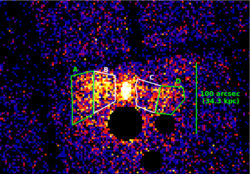
Figure 4: Image of 3C 386 with native 2.5″ pixels, highlighting the extraction regions for the inner (B & C) and outer (A & D) regions of the gas belt.

In an effort to establish the mechanism by which the belt was shaped, we further divide the belt region shown in Figure 2, into two smaller sub-regions. The sub-regions are shown in Figure 4, and are labelled as ‘inner’ and ‘outer’ regions corresponding to their position within the belt. Both inner and outer regions were fitted with the same models as the whole gas belt. When fitted to an APEC model, the temperature of the inner gas belt was found to be $0.73^{+0.08}_{-0.11}$ keV whilst the outer belt was found to have a temperature of $1.72^{+0.56}_{-0.36}$ keV.

If we assume the gas belt is a disk we are viewing side on, there would be some outer belt material in our line of sight in front and behind the inner region of the belt. To compensate for this and gain a more realistic measurement of the temperature of the inner belt, we fitted an APEC + APEC model to the inner belt spectra. The first APEC has a temperature fixed to the best-fit value measured from the outer belt fit, and its normalisation is set to accommodate the outer gas assuming a disk geometry. The second APEC, corresponding to only the inner material is then fitted to a temperature of $0.62^{+0.12}_{-0.10}$ keV, somewhat lower than before. Once we established the temperatures of the two gas components, we performed a second APEC + APEC fit, this time to the entire gas belt. In this fit the temperatures were fixed at the inner and outer component values. This enabled us better to gauge the spatial extent of each temperature component, as discussed further in Section 4.2.2.

Each subdivision of the belt can alternatively be fitted to an absorbed power law, with $\Gamma=2.70^{+0.37}_{-0.28}$ for the inner gas belt, and $\Gamma=2.10^{+0.17}_{-0.16}$ for the outer gas belt. A combination of an absorbed APEC and a power law finds the temperature of the inner gas belt $0.67^{+0.10}_{-0.09}$ keV and the outer gas belt $1.56^{+0.41}_{-0.18}$ keV, and the power law 1 keV normalisations are an order of magnitude smaller than those of the thermal components. Each fit described above has a fixed metal abundance with respect to solar of $Z_{\odot}=0.3$. Further details can be found in Table 3.

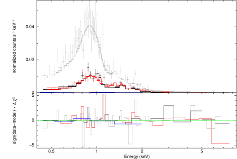
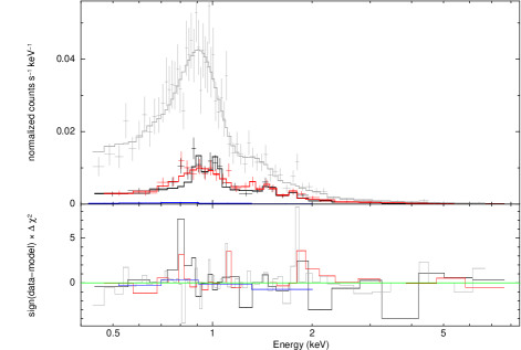
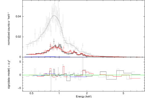
Figure 5: XMM-Newton spectra extracted from the whole gas belt, fitted to the background model plus an APEC component in the top panel, an absorbed power law in the middle panel and an APEC + power-law model in the bottom panel. The lower panel in each fit show the $\chi^{2}$ residuals. In each panel, black, red, and grey correspond to MOS1, MOS2, and pn data, respectively.

We also performed a second APEC fit on the inner and outer gas belts, this time allowing the metal abundances in each region to vary along with the other parameters. We find no significant change in temperature, with metal abundance of $Z_{\odot}=0.12^{+0.12}_{-0.05}$ and $Z_{\odot}=0.68\pm 0.49$ in the inner and outer regions respectively.

For the discussion, we assume that the gas belt is entirely of thermal origin, since any power law contribution is small.

The volume of the gas belt was estimated as $49\times 10^{3}$ kpc³, by assuming it is part of a disk of radius 83″($\sim 30$ kpc) and thickness 50″($\sim 18$ kpc). The radius and thickness of the disk were estimated assuming that the disk is seen edge-on.

Model parameter	Whole gas belt	Inner belt	Outer belt
APEC
$kT$ (keV)	0.94${}^{+0.04}_{-0.05}$	$0.73^{+0.08}_{-0.11}$	$1.72^{+0.56}_{-0.36}$
$10^{14}N$ ($10^{9}$ cm-5)	3.83${}^{+0.63}_{-0.62}$	$1.78^{+0.43}_{-0.42}$	$2.22\pm 0.70$
$\chi^{2}$/dof	95.0/98	75.6/82	70.4/80
APEC + APEC
$kT_{1}$ (keV)	1.72 (fixed)	1.72 (fixed)	-
$10^{14}N_{1}$ ($10^{9}$ cm-5)	$3.92\pm 0.56$	1.04 (fixed)	-
$kT_{2}$ (keV)	0.62 (fixed)	$0.62^{+0.12}_{-0.10}$	-
$10^{14}N_{2}$ ($10^{9}$ cm-5)	$1.83\pm 0.32$	$1.01^{+0.47}_{-0.46}$	-
$\chi^{2}$/dof	95.8/101	75.2/78	-
power law
$\Gamma$	2.33$\pm$0.11	$2.70^{+0.37}_{-0.28}$	$2.10^{+0.17}_{-0.16}$
$S_{\rm 1~{}keV}$ (nJy)	10.49${}^{+1.57}_{-1.55}$	$5.01^{+1.37}_{-1.34}$	$4.20^{+1.20}_{-1.14}$
$\chi^{2}$/dof	112.6/106	93.0/90	85.5/88
APEC + power law
$kT$ (keV)	0.90${}^{+0.06}_{-0.10}$	$0.67^{+0.10}_{-0.09}$	$1.56^{+0.41}_{-0.18}$
$10^{14}N_{\rm apec}$ ($10^{9}$ cm-5)	3.47${}^{+0.64}_{-0.39}$	$1.78^{+0.33}_{-0.34}$	$2.40^{+0.70}_{-0.88}$
$\Gamma$	1.34${}^{+0.32}_{-0.39}$	$1.24^{+0.63}_{-0.20}$	$1.07^{+1.06}_{-0.43}$
$N_{\rm power~{}law}$	0.38${}^{+0.32}_{-0.30}$	$0.22^{+0.13}_{-0.11}$	$0.04^{+0.26}_{-0.04}$
$(10^{-5}$cm-2s-1keV${}^{-1})$
$\chi^{2}$/dof	84.5/95	94.5/79	75.0/77

Table 3: Best fit parameters of the emission from across the whole gas belt, the inner gas belt and the outer gas belt of 3C 386. Models fit are an absorbed APEC, power law and APEC plus power law. Metal abundances in the APEC, APEC + APEC and APEC + power law fits are fixed at $Z_{\odot}$ = 0.3. Errors are quoted for a 90% confidence range.

4.2.2 Physical properties of the gas belt

The gas belt of 3C 386 is well described by a thermal model. Using the fitted parameter values along with the estimated volume we calculate the pressure and total mass of the gas belt following the methods described in Worrall & Birkinshaw (2006). The emission measure, defined in terms of the normalisation factor given by the APEC model, $N$, is given by

$$\centering 10^{14}N=\frac{(1+z)^{2}\int n_{\rm e}n_{\rm p}dV}{4\pi D_{\rm L}^{2}}\@add@centering$$ (1)

where $D_{\rm L}$ is the luminosity distance in cm, $V$ is the volume in cm³ and $n_{\rm p}$ is the proton density in cm^-3. With normal cosmic values for element abundances, the proton number density for a region of uniform density is given by

$$\centering n_{\rm p}\approx\sqrt{\frac{10^{14}N4\pi D_{\rm L}^{2}}{(1+z)^{2}1.18V}}\@add@centering$$ (2)

If the proton density is constant over the volume, the pressure can then be found by

$$P=3.6\times 10^{-10}n_{\rm p}kT\quad\text{Pa}$$ (3)

where $n_{\rm p}$ is in units of cm^-3 and $kT$ is in units of keV (Worrall et al., 2012).

A summary of results for the gas belt are given in Table 4. The densities and pressures in the gas belt correspond to the average density and average pressure over the region of the spectral extraction. The masses calculated in Table 4 for the inner and outer belt were found using the APEC + APEC fit for the inner region and the APEC fit for the outer region. The distinction between the inner and outer belt was made at approximately the mid-point in the belt on either side of the core. We tested that this distribution of gas is roughly correct, by fitting an APEC + APEC to the entire belt with each APEC fixed at the inner and outer temperature. When doing this, we find a mass for the inner belt of log$(M/M_{\odot})=8.8\pm 0.1$ and a mass for the outer belt of log$(M/M_{\odot})=9.1\pm 0.1$. These masses are similar to those in Table 4, supporting our choice of the relative spatial extents of the inner and outer belt regions.

Parameter	Gas belt	Inner belt	Outer belt
$kT$ (keV)	0.94${}^{+0.04}_{-0.05}$	$0.62^{+0.12}_{-0.10}$	1.72${}^{+0.56}_{-0.36}$
Volume (kpc3)	$49\times 10^{3}$	$13\times 10^{3}$	$36\times 10^{3}$
$n_{\rm p}$ (m-3)	$1250\pm 200$	$1200\pm 100$	$1300\pm 100$
$P$ (10-13 Pa)	$4.1\pm 0.2$	$2.8^{+0.8}_{-0.9}$	8.2${}_{-1.8}^{+2.8}$
log($M/M_{\odot}$)	$9.2\pm 0.1$	$8.6\pm 0.1$	$9.0\pm 0.1$
$\bar{r}$ (kpc)	15	10	21

Table 4: Temperature, density, and mass of the X-ray emission for the belt estimated from the XMM-Newton observations. $\bar{r}$ corresponds to the average distance from the core for regions of the gas belt.

4.3 Lobes

The XMM-Newton spectra for the radio lobes were extracted from two elliptical regions north and south of the gas belt. Contaminating sources (holes seen in Figure 2) are excluded. Also in Figure 2, there is some excess flux visible from the wings of the PSF of an excluded bright GALEX source. These remaining counts contribute a small fraction of the total counts in the southern lobe, and have no significant impact on the spectral fits. The net count rates for each detector for each lobe are given in Table 2. The lobes were fitted separately. We performed a combined fit of the MOS and pn spectra. The source emission in both lobes is best fitted by a power law with fixed Galactic absorption. These fits find a photon index of $\Gamma=2.02^{+0.23}_{-0.21}$ ($\alpha_{X}=1.02^{+0.23}_{-0.21}$) for the northern lobe and $\Gamma=1.57^{+0.12}_{-0.11}$ ($\alpha_{X}=0.57^{+0.12}_{-0.11}$) for the southern lobe. See Table 5 for details. The difference in the spectral indices of these lobes is probably caused by different amounts of foreground and background gas along the line of sight. When both lobes are fit together we find $\alpha_{X}=0.73^{+0.11}_{-0.07}$. Using measurements of flux density from the lobes of 3C 386 between 178 and 5000 MHz collected from the NASA/IPAC Extragalactic Database (NED), we find a spectral index $\alpha_{\rm r}=0.72\pm 0.16$. The X-ray and radio indices agree within measurement errors.

Model parameter	North lobe	South lobe
$N_{\rm H}$ (1021 cm-2)	1.81 (fixed)	1.81 (fixed)
$\Gamma$	2.02${}^{+0.23}_{-0.21}$	1.57${}^{+0.12}_{-0.11}$
$S_{\rm 1~{}keV}$ (nJy)	7.05${}^{+1.40}_{-1.39}$	6.28${}^{+0.76}_{-0.82}$
$\chi^{2}$/dof	227.5/268	295.0/310
1.4 GHz Radio flux density (Jy)	$2.97\pm 0.31$	$1.39\pm 0.21$

Table 5: Summary of the power law model fitting to the north and south lobes of 3C 386, along with measured radio flux densities. The Galactic neutral hydrogen column density is frozen for all fits. Errors are quoted for a 90% confidence range.

The lobes were also fitted to APEC models. With a fixed abundance of 0.3$Z_{\odot}$, the temperatures are found to be 3.3 $\pm$ 0.8 keV for the northern lobe and 6.2 $\pm$ 1.3 keV for the southern lobe. These temperatures are unrealistically high for 3C 386, as they are more consistent with those expected in a cluster environment. No evidence from either the X-ray surface brightness or the galaxy’s environment suggests that 3C 386 resides in a cluster. We therefore conclude that the emission in the lobes is non-thermal, even though the $\chi^{2}$ values for the thermal fits are acceptable.

Approximating oblate ellipsoids for the northern and southern lobes, we estimate the volumes corresponding to X-ray emission to be $81\times 10^{3}$ kpc³ and $42\times 10^{3}$ kpc³, respectively. The volume for the southern lobe has been corrected down to account for the excised regions. The 1.4 GHz VLA radio flux density was measured to be $2.97\pm 0.31$ Jy for the northern lobe and $1.39\pm 0.21$ Jy for the southern lobe over the same areas used for the X-ray spectral extraction.

4.4 The Core

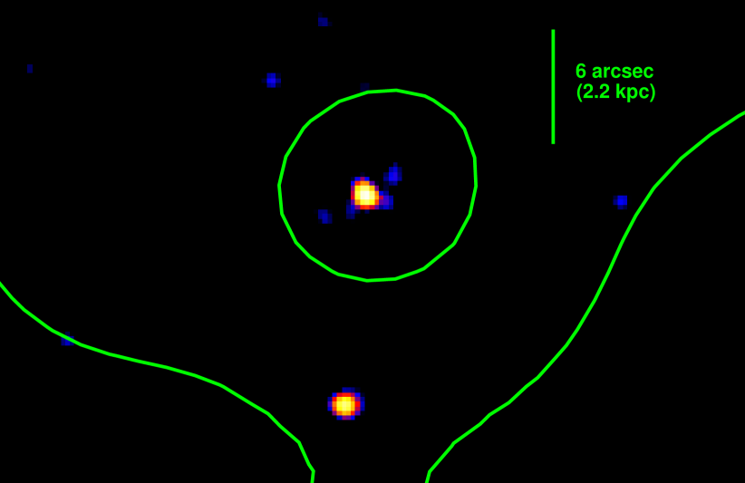
Figure 6: 0.5-7.0 keV Chandra image of the core of 3C 386 with 0.246″pixels, smoothed with a Gaussian of standard deviation 0.37″. Contours are of a 1.4 GHz VLA map 10, 15 mJy/beam (5.8″ beam). The northern X-ray component within the radio map’s centre corresponds to the radio nucleus, while the component to the south corresponds to stellar emission. These two components are confused in the XMM-Newton images.

The core is a superposition of the radio nucleus and an F7-type Galactic star. These two components can be seen in the Chandra observation of 3C 386 (see Figure 6), with a northern component corresponding to the radio nucleus, and a separate southern component corresponding to emission from the star. Despite this, the spectrum of the core was extracted from a circular region with radius 12.5″. The spectral data from the core were fitted to an absorbed power law with fixed Galactic absorption of $N_{\rm H}=1.81\times 10^{21}$ cm^-2. The best-fit photon index was found to be $\Gamma=2.11^{+0.26}_{-0.25}$ and the best-fit 1 keV flux density corresponds to $S_{\rm 1~{}keV}=3.01^{+0.82}_{-0.85}$ nJy, with $\chi^{2}/\text{dof}=126.1/133$. The spectral fit shows some indication of structured residuals between 0.6 and 0.9 keV. There is no evidence of excess absorption and results are consistent with the cores of other FRI radio galaxies (Evans et al., 2006). The 2-10 keV X-ray luminosity of the core is $6.54\times 10^{39}$ ergs s^-1, which is roughly consistent with the value obtained by Ogle et al. (2010). Our derived X-ray luminosity is an upper limit because of contaminating emission from the star.

4.5 Extended Group Gas

Group-scale gas is evident in the XMM-Newton data, although was not necessarily expected given what is known of the galaxy environment (Section 1.1). The spectrum of this component was first extracted from an annulus surrounding the galaxy, extending between 100″  to 230″ from the core, and so beyond the belt and mostly beyond the radio lobes. To check the consistency of our results we also extracted a spectrum from a small rectangular region of less than 6% of the whole area (2.1 square arcmin, 2′ to the southwest of the core) which had good coverage on all three EPIC detectors. The results of the fit from the smaller rectangular region are used as a method of testing the reliability of the fit from the larger annulus, as there is often difficulty in consistently modelling the XMM-Newton background over large detector areas. The background in both of the extracted regions was modelled as described in Section 4.1. The data were fitted to an APEC model. For the annulus extraction, the temperature of the group is poorly constrained, with the best-fit temperature too high for the X-ray luminosity and inferred richness of the group. We have therefore fixed the temperature at 1.4 keV, which is roughly the $1\sigma$ lower bound. How this model fits the data for the group gas is shown in Figure 7, with parameter values given in Table 6. The rectangular region produces a temperature of 1.72${}^{+4.59}_{-0.94}$ keV, which is consistent with our temperature choice for the entire annulus. Although the errors on the measured temperatures are large, the XMM-Newton data support the existence of a component of extended emission of group scale and temperature.

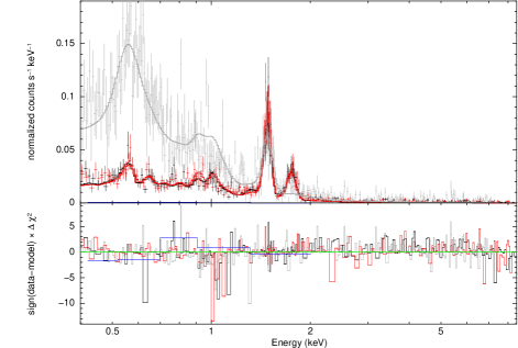
Figure 7: XMM-Newton spectra extracted from an annulus of group gas lying between 100″and 230″ from the core of 3C386, fitted with an APEC + background model. The lower panel shows the $\chi^{2}$ residuals. Black, red, and grey correspond to MOS1, MOS2, and pn data, respectively.

Model parameter	Group gas
$kT$ (keV)	1.4 (fixed)
$10^{14}N$ ($10^{9}$ cm-5)	$5.68^{+1.68}_{-1.89}$
$\chi^{2}$/dof	713.0/707

Table 6: Summary of the APEC fitting to the group gas surrounding 3C 386. The Galactic neutral hydrogen column density is frozen for all fits. Metallicity is fixed to 0.3$Z_{\odot}$. Errors are quoted for a 90% confidence range.

To investigate the radial profile of the group emission, counts were extracted from the pn detector from annuli of width 25″. We found a profile that decreased with increasing radius out to about 3.8 arcmin, at which point it flattened. This was taken to indicate the point at which the group emission falls significantly below the background. We used this information to subtract a background from each of the inner bins. The lobes and any additional point sources inside the annuli were masked so that only counts from group emission were counted. The resulting background-subtracted vignetting-corrected radial profile of X-ray gas surrounding 3C 386 is shown in Figure 8.

The radial profile can be a fitted with a $\beta$-model. We used $\chi^{2}$ fitting to establish the best fit to the model, with $\beta$ limited between 0.4 and 1.2 and find a best fit with $\beta=1.2^{\rm+unknown}_{-0.8}$, core radius, $r_{\rm cx}=91^{+56}_{-82}$ kpc and central counts, $B_{o}=140^{+460}_{-65}$. The best fit $\chi_{\rm min}^{2}=0.8$, with errors on each interesting parameter calculated to 90% confidence within $\chi^{2}_{\rm min}+2.7$ allowing the other parameters to vary. the fitted core radius is $r_{\rm cx}=30$ kpc. This is similar to the length of the gas belt, and so while group gas is detected out to 80 kpc, the gas belt lies within its core radius. Using equation 10 from Birkinshaw & Worrall (1993), the central proton density in cm^-3 from this model profile can be calculated.

$$\eta_{po}=\frac{2.45(1+z)^{3}}{a^{\frac{3}{2}}}\sqrt{\frac{B_{o}f\Gamma(3\beta)}{t\theta_{\rm cx}D_{\rm L}\Gamma(3\beta-0.5)}}$$ (4)

where $B_{o}$ is the central brightness in count arcmin^-2, $a$ is the number of radians per arcmin, $f$ is a calibration quantity equivalent to 1 ct/s in cm^-5 for a fitted xspec normalisation, $t$ is the exposure time, $\theta_{\rm cx}$ is the core radius in arcmin and $D_{\rm L}$ is the luminosity distance in cm.

Using this central proton density, the gas mass contained within multiples of the core radius can be calculated using the following equation:

$$M(r\leq kr_{\rm cx})=\frac{4k^{3}\pi m_{\rm H}\eta_{\rm po}r_{\rm cx}^{3}}{X}\int_{0}^{1}dx\,x^{2}(1+k^{2}x^{2})^{-\frac{3\beta}{2}}$$ (5)

where $x=r/kr_{\rm cx}$ is used as a substitution, $k$ is a multiple of the core radius, $m_{\rm H}$ is the mass of a hydrogen atom and $X$ is the cosmic abundance of hydrogen by mass. Using this integral we find the gas mass contained within $r_{\rm cx}$ is $3.0^{+4.5}_{-2.9}\times 10^{10}M_{\odot}$ and the gas mass contained within $2r_{\rm cx}$ is $8.1^{+12.0}_{-8.0}\times 10^{11}M_{\odot}$.

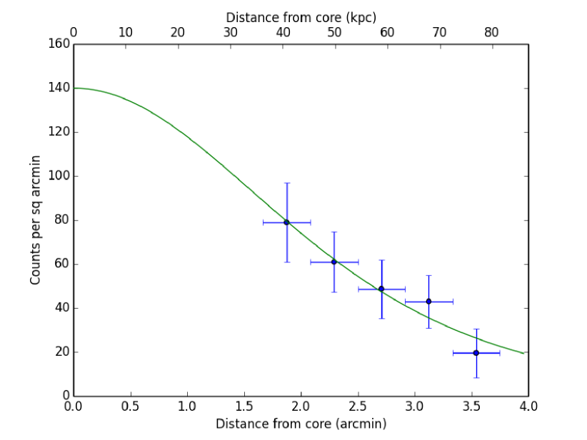
Figure 8: Vignetting-corrected, background subtracted radial profile of extended emission from the pn detector from  35 to  80 kpc from the core of 3C 386. Data have been filtered between 0.4-7.2 keV. The lobes and any additional point sources were masked in each annulus. The green line indicates a $\beta$-model where $\beta=1.2$ and $r_{\rm cx}=91$ kpc.

5 Discussion

Assuming that the belt is of constant density, we estimate the mass of gas it contains as log($M/M_{\odot})=9.2\pm 0.1$. When calculating the belt mass, we have continued to exclude the core from the volume. Were the core included, there would be an additional 4% of mass, which is less than the error quoted. This mass is similar to the average gas mass contained within 50 kpc of early-type galaxies (Anderson et al., 2013), despite being contained within a radius roughly half that distance. Furthermore, K-band measurements from 2MASS give $L_{\rm K}=1.6\times 10^{10}L_{\odot}$ for 3C 386. This is below the average range for early-type galaxies in Table 4 of Anderson et al. (2013), and so we would expect even less gas mass in 3C 386, around $2\times 10^{8}M_{\odot}$ (based on Su et al. 2015). The results suggest that 3C 386’s gas mass has been enhanced, presumably by gas originating in the group.

In Table 7 we estimate some physical parameters extrapolated from the observed group gas at roughly the distances of the inner and outer belt. These values are derived from an extrapolation to small radii using parameters from the radial profile discussed in Section 4.5.

$r$ (kpc)	$n_{\rm p}$ (m-3)	$P$ ($10^{-13}$ Pa)	$M(<r)\,(M_{\odot})$	$S$	$S_{\rm belt}$
				(keV cm2)	(keV cm2)
0	$610^{+2000}_{-260}$	$3.1^{+13}_{-1.3}$	-	$190^{+600}_{-50}$	-
10	$600^{+2000}_{-250}$	$3.0^{+13}_{-1.3}$	$1.5^{+2.3}_{-1.4}\times 10^{8}$	$200^{+600}_{-50}$	$50^{+10}_{-15}$
21	$560^{+1800}_{-240}$	$2.8^{+12}_{-1.2}$	$1.4^{+2.1}_{-1.3}\times 10^{9}$	$200^{+600}_{-40}$	$130^{+40}_{-30}$
60	$320^{+1100}_{-140}$	$1.6^{+6.9}_{-0.7}$	$2.3^{+3.5}_{-2.2}\times 10^{10}$	$300^{+1000}_{-70}$	-

Table 7: Density, pressure and pseudo-entropy (estimated using $kT/n_{\rm p}^{2/3}$) of the group gas extrapolated to radii appropriate for the inner belt (10 kpc) and outer belt (21 kpc). The inner and outer gas belt pseudo-entropy are also given.

Using density and temperature we can estimate cooling timescales, $\tau_{\rm cool}$. Based on the cooling curves calculated by Worrall & Birkinshaw (2006, their Figure 5), we estimate $\tau_{\rm cool}\sim 5$ Gyr for the gas belt in 3C 386.

5.1 Physical parameters of the lobes

The spectra of the X-ray lobes are well described by an absorbed power law (Table 5). As described in Section 4.3 the agreement between the X-ray and radio spectral indices is consistent with the interpretation of the X-ray power-law component originating from inverse-Compton (IC) emission from a population of electrons which are also producing synchrotron radio emission.

Using the volumes estimated in Section 4.3 and referring to Worrall & Birkinshaw (2006), we find a minimum energy magnetic field $B_{\rm me}=0.67$ nT for the northern lobe, and $B_{\rm me}=0.65$ nT for the southern lobe. These were estimated assuming a filling factor of unity, no relativistic protons and no relativistic bulk motions. Minimum-energy pressure, $P_{\rm me}$, is also given in Table 8.

Parameter	North lobe	South lobe
$B_{\rm me}$ ($10^{-10}$ T)	6.7	6.5
$P_{\rm me}$ ($10^{-13}$ Pa)	1.3	1.2
$B_{\rm iC}$ ($10^{-10}$ T)	2.7	1.8
$P$ ($10^{-13}$ Pa)	3.5	5.9
$u_{\rm B}$ ($10^{-13}$ J m-3)	0.3	0.1
$u_{\rm p}$ ($10^{-13}$ J m-3)	10.3	17.6

Table 8: Physical parameters calculated based on the X-ray emission from the lobes of 3C 386. $u_{\rm B}$ and $u_{\rm p}$ correspond to the energy density in the magnetic field and the energy density in particles respectively.

We also calculate the magnetic field and pressures in the lobes assuming all X-ray emission from the region is produced by the IC mechanism. Using this method we find lower magnetic fields in the lobes, with $B_{\rm iC}=0.27$ nT in the north lobe and $B_{\rm iC}=0.18$ nT in the south lobe. The pressures, $P$, in the lobes are found to be 3 and 5 times larger than those implied by the minimum-energy assumption. A discrepancy of a factor $\sim 3$ between $B_{\rm me}$ and $B_{\rm iC}$ for IC-emitting radio lobes is common (Croston et al., 2005).

5.2 Model

We have argued that there is too much gas in the belt for it to have originated entirely in the host galaxy. We suggest instead that it is being formed by a buoyancy-driven inflow from the gas atmosphere of the group on to a surviving cold core remnant of the pre-AGN atmosphere.

When the AGN of 3C 386 was at the height of its activity, it would have been feeding the radio lobes with jets, causing the lobes to expand into the intragroup gas. The AGN now appears to be driving no significant jets into the lobes, although it continues to show a low level of activity. The lobes are now rising buoyantly through the group medium away from the host galaxy, at a fraction of the sound speed in the group gas ($c_{\rm s}\sim$600 km s^-1). As the lobes rise, gas from the group atmosphere must flow back between the lobes, and we interpret the outer gas belt as the re-accumulated group atmosphere that has been developed by this flow. This is illustrated in Figure 9.

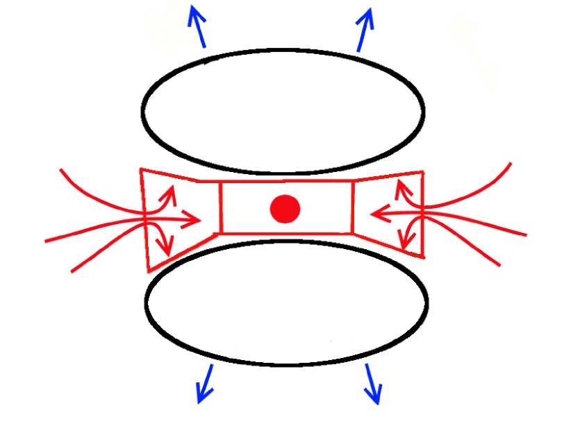
Figure 9: Once the radio source has become passive, the buoyant lobes rise through the ambient medium. Their motion through the group gas causes a ‘buoyancy-driven inflow’ of gas, which forms the outer gas belt. This inflow is directed towards the relic cool core of 3C 386.

The temperature structure of the belt supports this interpretation. The outer belt is hotter than the inner belt, with a temperature of about 1.7 keV, similar to that of the group gas. In the inner part of the belt the gas is cooler, at about 0.6 keV. The cooling time in the belt gas is far longer than the flow time from the edge to the centre of the belt (5 Gyr, compared to $\sim$50 Myr), so it is not cooling that causes the central temperature to be lower. It is possible that the inner belt gas is representative of the initial state of the group gas. Its low pseudo-entropy implies it is old, unheated group gas with a small ($\leq$10%) component of host galaxy gas. This is also supported by the morphology of the X-ray emission in the outer belt region. The density structure argues against the belt having arisen from the lobes acting on a pre-existing gas structure, as if this were the case, the inner belt would be denser than the outer.

Figure 2 seems to show that the gas belt has a sharp edge, which might not be expected from a buoyancy-driven inflow. However, a plot of the counts as a function of distance across the belt (Figure 10) reveals a more gradual change in the number of counts with distance from the core.

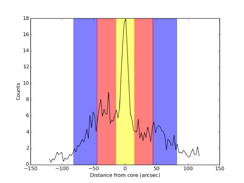
Figure 10: Background subtracted, exposure corrected counts as a function of distance from the core across a 20″  slice of the gas belt and its surrounding group medium. Colored region indicates the extent of the gas belt region shown in Figure 2, where blue corresponds to the outer belt, red corresponds to the inner belt and yellow corresponds to the core.

There are some remaining issues with our interpretation of the gas belt. First, the mass of gas in the belt $\sim 2\times 10^{9}M_{\odot}$, is about 10% of the total mass of the group gas within a sphere encompassing the radio lobes. The efficiency of collection of group gas into the belt region is unexpectedly high, and would correspond to a high mass flow rate, $\sim 40M_{\odot}$ yr^-1, into the belt. A redshift survey of 3C 386’s group would be useful to help improve our understanding of the extent and composition of the group as currently little is known. This may help identify whether a merger in this group helped reshape the gas distribution.

Second, the entropy of gas in the inner belt is significantly lower than that of the group gas, but the cooling time for the belt gas is too long for it to have cooled significantly over the lifetime of the radio source. The cold gas must therefore predate the radio activity, and the high mass means that it must be residual cool gas from the group. The group is poor in galaxies, consistent with the low gas temperature in the inner belt. The higher present temperature of the group gas and outer belt can then be interpreted as resulting from drastic heating driven by 3C 386 - the temperature difference between the inner belt and group roughly matches the heating that the lobes can provide. At the new temperature of the group, we expect much of the gas to escape. The system was previously in hydrostatic equilibrium at $\sim 0.7$ keV and is now at a temperature of at least 1.4 keV which could result in the group scale atmosphere being blown away. To test this, we calculate the total mass of the group contained within a specified radius using the following equation (Worrall & Birkinshaw, 2006):

$$M_{\rm tot}(<r)=\frac{3\beta kTr^{3}}{G\mu m_{\rm H}(r^{2}+r_{\rm cx}^{2})}$$ (6)

To a radius of 80 kpc, this gives a total group mass of $6.5^{+18}_{-6.4}\times 10^{12}M_{\odot}$. This is typical for galaxy groups (Mulchaey, 2000). We then find a gas mass fraction of $0.01^{+0.02}_{-0.005}$. This is much smaller than an expected cosmological value of about 0.17 (Planck Collaboration et al., 2015). Based on the size of the lobes and the sound speed in the group atmosphere, the age of the current outburst is 50 Myr. The sound speed of the gas is roughly equal to the escape velocity of the group, and it would take around 100 Myr for all the gas to flow out of the group. From these numbers, it is possible that a substantial fraction of the gas in the group has escaped due to heating by the radio source. It is also possible that multiple outbursts have been involved. Traces of a previous outburst may be sought in a low-frequency spectral index map, though we note that existing low frequency data show a relatively flat radio spectrum. Alternatively, the total mass of the 3C 386 group could be overestimated. Equation 6 applies only if the system is in hydrostatic equilibrium, whereas the 3C 386 system could be far from equilibrium if an inflow is present. If the total mass of the group is 10 times lower, so that the baryonic mass fraction is more normal, the total mass becomes of order a single galaxy mass, presumably the 3C 386 host galaxy itself.

If we consider the work done by the lobes and calculate the bubble enthalpy ($4PV\approx 6\times 10^{51}$ J) and compare this to the thermal energy of all the gas out to the radius of the lobes ($E=1.5^{+4.7}_{-1.4}\times 10^{52}$ J), we see that within errors, the values are equal. This provides a lower limit to the total energy of the outburst, although an extended supersonic phase could increase this substantially.

Finally, the outer belt appears overpressured relative to the inner belt and the radio lobes, although its entropy is close to that of the group gas. A high pressure in this region is unexpected, since the buoyant motion of the lobes should generate only small pressure imbalances and slow gas flows back towards the 3C 386 galaxy. The geometry of the belt is uncertain. For our calculations, we have assumed that the belt is a flat disk of constant height. However, looking at Figure 4, it is apparent that the outer belt splays outwards from the inner belt. This splaying could lead to the volume of the outer belt increasing by a factor of 2. The pressure in the outer belt would then fall to $5.8^{+1.5}_{-1.4}\times 10^{-13}$ Pa, bringing the outer belt closer to pressure balance with the inner belt, with any remaining imbalance attributable to the dynamics in the system.

Additionally, we are limited by our current fit of the group gas temperature, having had to fix this parameter at the lower bound of its fitted range. Current X-ray missions are unlikely to be able to improve the observational situation. Future missions, such as ATHENA, with its significantly improved sensitivity, may be needed to constrain better the properties of the group gas.

6 Conclusion

We have reported measurements of the extended X-ray emission in the low-excitation radio galaxy 3C 386. We find that emission from the lobes is consistent with the interpretation of the X-ray power-law component originating from IC emission. The implied departure from equipartition of the lobes is comparable to the range seen in other sources.

We find that the X-ray emission from the gas belt in 3C 386 is most likely thermal, with an average temperature of 0.94${}^{+0.04}_{-0.05}$ keV across the whole of the belt. We find that the belt displays a clear temperature structure, with the gas closer to the core cooler than the gas closer to the surrounding group medium. We interpret this temperature structure as indicating that the belt was likely formed by a combination of gas components. In the outer belt a ‘buoyancy-driven inflow’ of part of the group-gas atmosphere, caused by the buoyant rising of the radio lobes through the ambient medium once the radio source became passive, is causing hot group gas to flow towards a relic cool core. This relic cool core is formed of old group gas, predating the radio activity in 3C 386.

It is possible that this inflow could lead to a resupply of fuel to the AGN, caused by gas reaching the parsec-scale regions surrounding the central black hole, which would lead to 3C 386 resuming a high level of radio activity in the future.

7 Acknowledgements

The authors thank the anonymous referee for their thorough report with many useful suggestions. This research has made use of the NASA/IPAC Extragalactic Database (NED) which is operated by the Jet Propulsion Laboratory, California Institute of Technology, under contract with the National Aeronautics and Space Administration. RTD thanks the STFC for their support.

References

- Anderson et al. (2013) Anderson M. E., Bregman J. N., Dai X., 2013, ApJ, 762, 106
- Birkinshaw & Worrall (1993) Birkinshaw M., Worrall D. M., 1993, ApJ, 412, 568
- Buttiglione et al. (2009) Buttiglione S., Capetti A., Celotti A., Axon D. J., Chiaberge M., Macchetto F. D., Sparks W. B., 2009, AAP, 495, 1033
- Croston et al. (2005) Croston J. H., Hardcastle M. J., Harris D. E., Belsole E., Birkinshaw M., Worrall D. M., 2005, ApJ, 626, 733
- Evans et al. (2006) Evans D. A., Worrall D. M., Hardcastle M. J., Kraft R. P., Birkinshaw M., 2006, ApJ, 642, 96
- Feigelson & Berg (1983) Feigelson E. D., Berg C. J., 1983, ApJ, 269, 400
- Hardcastle et al. (2007) Hardcastle M. J., Kraft R. P., Worrall D. M., Croston J. H., Evans D. A., Birkinshaw M., Murray S. S., 2007, ApJ, 662, 166
- Ineson et al. (2015) Ineson J., Croston J. H., Hardcastle M. J., Kraft R. P., Evans D. A., Jarvis M., 2015, MNRAS, 453, 2682
- Leahy & Perley (1991) Leahy J. P., Perley R. A., 1991, AJ, 102, 537
- Lynds (1971) Lynds R., 1971, ApJL, 168, L87
- Madrid et al. (2006) Madrid J. P., Chiaberge M., Floyd D., Sparks W. B., Macchetto D., Miley G. K., Axon D., Capetti A., O’Dea C. P., Baum S., Perlman E., Quillen A., 2006, ApJS, 164, 307
- Mannering (2013) Mannering E., 2013, Unpublished PhD thesis, University of Bristol
- Mannering et al. (2013) Mannering E., Worrall D. M., Birkinshaw M., 2013, MNRAS, 431, 858
- McNamara & Nulsen (2007) McNamara B. R., Nulsen P. E. J., 2007, ARAA, 45, 117
- Miller et al. (2002) Miller N. A., Ledlow M. J., Owen F. N., Hill J. M., 2002, AJ, 123, 3018
- Miller et al. (1999) Miller N. A., Owen F. N., Burns J. O., Ledlow M. J., Voges W., 1999, AJ, 118, 1988
- Mulchaey (2000) Mulchaey J. S., 2000, ARA&A, 38, 289
- Ogle et al. (2010) Ogle P., Boulanger F., Guillard P., Evans D. A., Antonucci R., Appleton P. N., Nesvadba N., Leipski C., 2010, ApJ, 724, 1193
- Planck Collaboration et al. (2015) Planck Collaboration Ade P. A. R., Aghanim N., Arnaud M., Ashdown M., Aumont J., Baccigalupi C., Banday A. J., Barreiro R. B., Bartlett J. G., et al. 2015, ArXiv e-prints
- Scheuer (1974) Scheuer P. A. G., 1974, MNRAS, 166, 513
- Smith et al. (2001) Smith R. K., Brickhouse N. S., Liedahl D. A., Raymond J. C., 2001, ApJ, 556, L91
- Snowden & Kuntz (2011) Snowden S. L., Kuntz K. D., 2011, Cookbook for Analysis Procedures for XMM-Newton EPIC MOS Observations of Extended Objects and the Diffuse Background (ftp://xmm.esac.esa.int/pub/xmm-esas/xmm-esas.pdf)
- Strom et al. (1978) Strom R. G., Willis A. G., Wilson A. S., 1978, AAP, 68, 367
- Su et al. (2015) Su Y., Irwin J. A., White III R. E., Cooper M. C., 2015, ApJ, 806, 156
- Worrall & Birkinshaw (2006) Worrall D. M., Birkinshaw M., 2006, in Alloin D., ed., Physics of Active Galactic Nuclei at all Scales Vol. 693 of Lecture Notes in Physics, Berlin Springer Verlag, Multiwavelength Evidence of the Physical Processes in Radio Jets. p. 39
- Worrall et al. (2007) Worrall D. M., Birkinshaw M., Kraft R. P., Hardcastle M. J., 2007, ApJL, 658, L79
- Worrall et al. (2012) Worrall D. M., Birkinshaw M., Young A. J., Momtahan K., Fosbury R. A. E., Morganti R., Tadhunter C. N., Verdoes Kleijn G., 2012, MNRAS, 424, 1346
- Young et al. (2005) Young A., Rudnick L., Katz D., DeLaney T., Kassim N. E., Makishima K., 2005, ApJ, 626, 748