Physical parameters of IPHAS-selected classical Be stars.

We present a semi-automatic procedure to obtain fundamental physical parameters and distances of classical Be (CBe) stars, based on the Barbier-Chalonge-Divan (BCD) spectrophotometric system. Our aim is to apply this procedure to a large sample of CBe stars detected by the IPHAS photometric survey, to determine their fundamental physical parameters and to explore their suitability as galactic structure tracers. In this paper we describe the methodology used and the validation of the procedure by comparing our results with those obtained from different independent astrophysical techniques for subsamples of stars in common with other studies. We also present a test case study of the galactic structure in the direction of the Perseus Galactic Arm, in order to compare our results with others recently obtained with different techniques and the same sample of stars. We did not find any significant clustering of stars at the expected positions of the Perseus and Outer Galactic Arms, in agreement with previous studies in the same area that we used for verification.

1 Introduction

Classical Be (CBe) stars are main-sequence O, B and early A-type stars whose spectra show -or have shown- Balmer and other lines in emission. They are characterised by excess continuum emission in the ultraviolet, optical and infrared spectral ranges. Both the line and continuum emission arise from recombination processes in a hot, dense circumstellar decretion disk. The formation of these disks is not yet completely understood, although fast rotation, nonradial pulsations and magnetic fields are believed to be at their origin. A recent review of the nature of CBe stars and their main characteristics is presented by Rivinius et al. (2013).

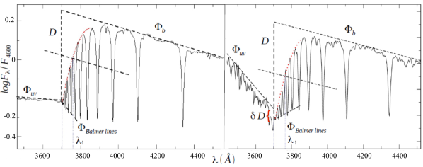
Figure 1: (a) Graphical explanation of the BCD $(D,\lambda_{1},\phi_{b},\phi_{uv})$ parameters in the spectrum of the B9.5V star HR4468; (b) determination of the BCD parameters of the emission line star IPHAS J002926.93+630450.2, with B9Ve spectral type. $\Phi_{Balmer\leavevmode\nobreak\ lines}$ is the line connecting the bottom of the higher Balmer lines, and $\delta D$ is the difference between the values of $D$ obtained from $\Phi_{Balmer\leavevmode\nobreak\ lines}$ and $\Phi_{uv}$.

In general CBe stars, have had relatively little time to move far away from their birthplaces as they are short-lived objects - particularly those of the earlier types. Being main-sequence or slightly evolved stars, they are unlikely to be embedded in their parental clouds. In addition, they are intrinsically bright, with absolute magnitudes ranging from $\sim$0 to $\sim-4$, enabling their detection across the whole Galactic Plane, at least in regions not affected by heavy interstellar absorption. As such, they are tracers relevant to the investigation of the spiral structure of the Galaxy.

The INT Photometric H$\alpha$ Survey of the Northern Galactic Plane (IPHAS, Drew et al. 2005; Barentsen et al. 2014) is a 1800 deg² imaging survey covering the entire northern Milky Way at $|b|<5^{o}$ in the $r$, $i$ and H$\alpha$ filters, using the Wide Field Camera (WFC) on the 2.5-metre Isaac Newton Telescope (INT) in La Palma. A first list of objects displaying H$\alpha$ emission was presented by Witham et al. (2008). Most of the objects from this list have been followed up spectroscopically, at $r<17$ mag., at some point between 2005 and 2012, leading to a database of low resolution spectra of 2627 objects. Preliminary analysis reveals that about 70% of this sample are CBe stars.

The general aim of this work is to obtain the fundamental physical parameters of the newly uncovered population of IPHAS CBe stars, which significantly increases the number of these objects known in the Galaxy. In addition, we aim to use this sample to contribute to the investigation of the spiral structure of the Galaxy in the northern hemisphere, using them as tracers and the standard techniques of spectroscopic parallax to measure their distances. These sources will likely obtain moderately accurate trigonometric parallaxes from Gaia in the near future. Therefore, their proper characterisation would also aid their future exploitation for more detailed studies of Galactic structure with Gaia data.

To deal with such a large set of spectra we have developed a semi-automatic procedure to obtain the relevant physical parameters of the CBe stars, including the spectral type and luminosity class, effective temperature, interstellar extinction and absolute magnitude. We have used the techniques and calibrations of the Barbier-Chalonge-Divan (BCD) spectrophotometric system (Barbier & Chalonge 1941; Chalonge & Divan 1952).

The aim of this paper is to describe the procedure we have developed to obtain CBe star astrophysical parameters from low resolution spectra, and to validate its results by comparing them with results obtained from different standard astrophysical techniques for samples of stars they have in common. A subsequent study, in preparation, will present the determination of the astrophysical parameters for the whole sample of the IPHAS CBe stars with available spectroscopy.

The paper is structured as follows: in Sect. 2 we describe the techniques of the BCD spectrophotometric system and their implementation in a semi-automatic procedure which allows us to analyse a large number of spectra efficiently, with little human intervention; in Sect. 3 we describe the spectroscopic data used for this work; in Sect. 4 we present the work we have undertaken to validate our procedure, by comparing our results with results for two samples of stars obtained with different observational data and standard astrophysical techniques; in Sect. 5 we revisit the inferred spatial distribution of the CBe stars in the direction of the Perseus Arm ($-1^{o}<b<4^{o}$, $120^{o}<l<140^{o}$), and compare the results with recent studies in the literature.

2 The BCD spectrophotometric system

The BCD spectrophotometric system was developed by Barbier & Chalonge (1941), and later by Chalonge & Divan (1952). The system is based upon measurable parameters around the Balmer discontinuity (BD), in the $3200-4600\ \AA$ spectral range. The basic parameters that describe the energy distribution around the BD are: $D$, the Balmer jump depth, given in dex, which is an effective temperature indicator; $\lambda_{1}$, the position of the Balmer discontinuity, given in $\AA$ as the difference from $3700\ \AA$, which is sensitive to the surface gravity; $\Phi_{b}$, a colour gradient which represent the slope of the Paschen continuum near the BD; and $\Phi_{uv}$, the slope of the Balmer continuum.

The BD is an easily visible spectral feature for stars ranging from early O to late F spectral types. A modern description of the BCD system, together with a presentation of its advantages compared to other spectroscopic systems, is given by Zorec et al. (2009).

In Fig. 1 we present a graphical description of how the BCD parameters are measured. The value of $D$ is calculated at $\lambda=3700\ \AA$, as $D=\log_{10}(F_{3700^{+}}/F_{3700^{-}})$, where $F_{3700^{+}}$ is the flux of the extrapolated Paschen continuum and $F_{3700^{-}}$ the corresponding flux on the Balmer continuum.

To measure the $\lambda_{1}$ parameter, the mean spectral position of the BD is obtained as the intersection between the spectral continuum and the average of the extrapolated Paschen and Balmer continua at $3700\ \AA$. The line that represents the average of the $\Phi_{b}$ and $\Phi_{uv}$ fluxes is determined by the points $\log F_{\lambda}-D/2$, in the Paschen continuum region at $\lambda=4000,4150$ and $4300\ \AA$ and $\log F_{3700}+D/2$ in the Balmer continuum at 3700 Å.

The parameters $D$ and $\lambda_{1}$ are independent of interstellar extinction, and allow the determination of the effective temperature and surface gravity by means of the calibration given by Zorec et al. (2009). The third parameter $\Phi_{b}$, which measures the slope of the Paschen continuum, is a function of both the effective temperature and the interstellar extinction, and can be used to measure the interstellar reddening by means of the expression:

$$A_{V}=3.1E(B-V)=2.1(\Phi_{b}-\Phi_{b}^{0})$$ (1)

From (Aidelman et al. 2012), where $\Phi_{b}^{0}$ is the intrinsic gradient obtained from $D$ and $\lambda_{1}$ by means of the calibration given in Chalonge & Divan (1973).

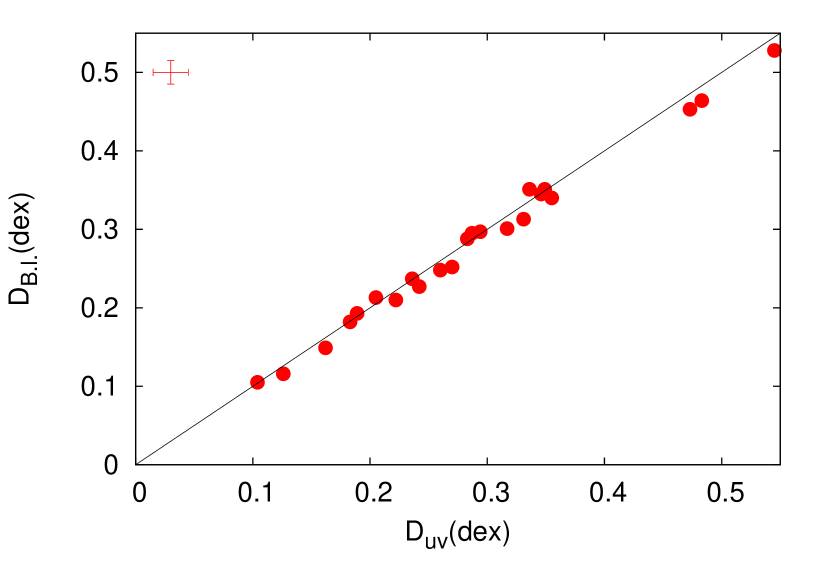
Figure 2: Comparison of the Balmer jump depth calculated for 23 absorption-line B-type stars, using both the ultraviolet continuum and the Balmer lines limit as explained in the text. At the left upper part it is shown the typical error in the determination of $D$, 0.015 dex.

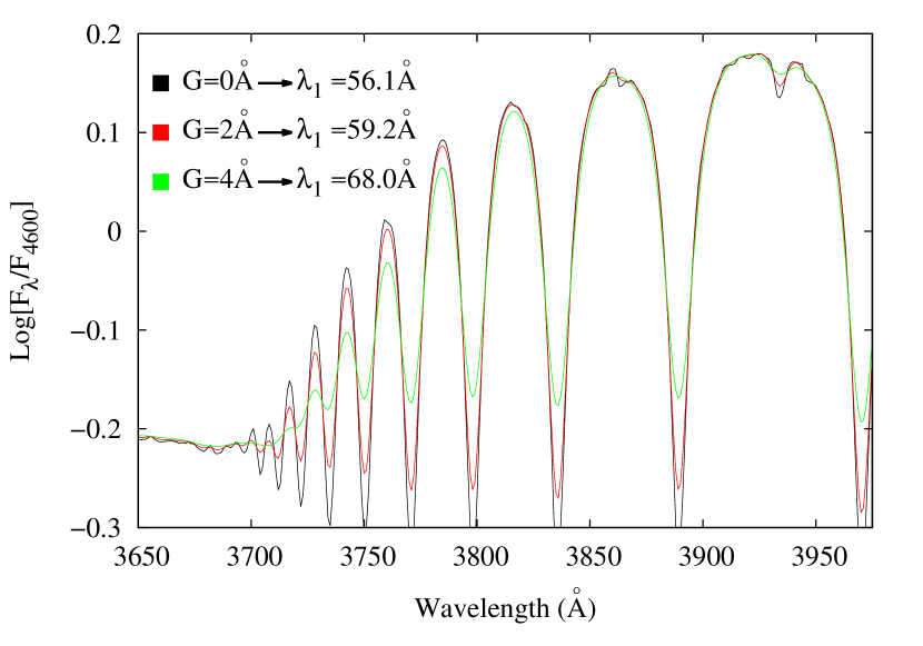
Figure 3: The region around the BD area of the standard B-type star HR4468. The black line represents the original spectrum, and red and green lines the spectrum convolved with Gaussian filters of $2\AA$ and $4\AA$ width respectively.

2.1 The determination of the photospheric Balmer discontinuity of Be stars

The procedure described above to determine the Balmer discontinuity depth is, however, in general not applicable to CBe stars. Due to the lower pressure of the circumstellar disc, a second Balmer jump exists for these objects in the ultraviolet region of the spectrum, which is either in emission or absorption (Kaiser 1989). In the case of emission, we extract the flux at $F_{3700^{-}}$ as the point where the bottom of the higher order Balmer line series merges into the continuum.

In Fig. 1b we illustrate this last procedure. To obtain the flux at $F_{3700^{-}}$, instead of using the extrapolated Balmer continuum $\Phi_{uv}$, we extrapolate the line traced through the bottom of the higher Balmer lines, which is labeled $\Phi_{Balmer\leavevmode\nobreak\ lines}$. In the case of non emission-line stars, both methods lead to the same $D$ values, as shown in Figs. 1a and 2, and in columns 6 and 7 of Table 2. The mean of the residuals between the two different measurement procedures is 0.010$\pm$0.007 dex, significantly smaller than the characteristic error of 0.015 dex associated with the measure of the $D$ parameter in the BCD system.

In the case of CBe stars, the value of $D$ obtained in this way is the true photospheric value, not affected by circumstellar emission or absorption in the Balmer and Paschen continua. The validity of this statement is fundamental for the applicability of the BCD system to the determination of the physical parameters of CBe stars, and hence in Appendix A we discuss this issue in detail.

2.2 Setting the spectral resolution

The original calibration of the stellar parameters in the BCD system was made empirically from spectra with a mean resolution of $\Delta\lambda\sim 8\ \AA$ at the BD. Although the $D$ parameter is independent of the resolution, the mean position of the BD, and hence the $\lambda_{1}$ parameter, varies with the spectral resolution. This effect is illustrated in Fig. 3, where we present the spectrum of the B-type star HR4486 at different resolutions.

Because the determination of astrophysical fundamental parameters proceeds with calibrations obtained with the original BCD parameters, to measure $\lambda_{1}$ we have to reduce the resolution of our spectra to the characteristic resolution of the original BCD spectrophotometric system. This is done by convolving the spectra with a Gaussian filter of the appropriate width, so that the resolution to apply the BCD formalism is obtained by

$$R_{F}=\sqrt{R_{I}^{2}+G^{2}}$$ (2)

where $R_{F}$ is the resolution required for the BCD method, $R_{I}$ is the initial resolution of the spectra, and $G$ is the width of the Gaussian filter.

Setting of the correct spectral resolution is a complex issue, and depends on the available set of data. In Sect. 3.3. we explain how we have selected the appropriate correction of the resolution for the spectra analysed in this work.

2.3 Absolute magnitudes and distances

Absolute magnitudes in the Johnson $V$ band (M_V) are directly obtained from the $D$ and $\lambda_{1}$ parameters by means of the calibration given in Table 3 of Zorec & Briot (1991). They are converted to absolute IPHAS $r$ magnitudes using the intrinsic $(V-R_{C})$ colours for dwarfs and giants supplied by Fabregat (in preparation), and assuming that Cousins $R_{C}$ and IPHAS $r$ magnitudes in the Vega system are identical within the errors involved in our procedure.

Distances are obtained by means of the standard spectroscopic parallax techniques, by comparing the absolute M_r magnitudes with the observed $r$ magnitudes supplied in the IPHAS Second Data Release (IPHAS DR2, Barentsen et al. 2014), corrected for the interstellar absorption and the circumstellar excess due to the added flux of the disk emission.

Intrinsic $r$ magnitudes corrected for interstellar absorption were computed using the relationship A_r = 0.84 A_V, from Fiorucci & Munari (2003). To correct for CBe circumstellar continuum emission we followed the method described in Sect. 3.3 of Raddi et al. (2013), which follows the earlier work by Dachs et al. (1988) that investigated the correlation between $EW(H\alpha)$ and the circumstellar colour excess $E^{cs}(B-V)$. The relations adopted in this work are

$$E^{cs}(B-V)\approx 0.02\frac{EW(H\alpha)}{-10\AA},$$ (3)

and

$$f_{D}=\frac{F_{D}}{F_{D}+F^{*}}\approx 0.1\frac{EW(H\alpha)}{-30\AA},$$ (4)

From these values we obtain the circumstellar emission in the $r$ band, $\Delta r$, by interpolating from Table 5 of Raddi et al. (2013). The $\Delta r$ correction applied for each source is given in Table 6.

2.4 Code principles

In order to analyse a large sample of spectra in a reasonable amount of time we have developed a semi-automatic procedure, only requiring user interaction to evaluate output diagrams at some important steps during the treatment of each spectrum. The basic inputs of the programme are the observed spectra, with the wavelength scale in $\AA$ and the flux in $ergs^{-1}cm^{-2}$, and a list with the names of the files containing each spectrum.

The pipeline used to treat each spectrum requires a series of inputs that the user provides as the analysis proceeds. The first step of the procedure is to ask the user for the dispersion of the spectra, and for the width $G$, in $\AA$, of the Gaussian filter that the spectra require in order to transform their resolution to the original resolution of the BCD system. This first step is valid for the whole run and applies to all the spectra in the list. The next step is the analysis of the spectra one by one. As each spectrum is presented for analysis, it is first thoroughly checked to establish its wavelength range and to detect possible recording flaws.

One of the steps which requires user interaction is the wavelength scale, whose possible variations, caused either by errors in the wavelength calibration or by the radial velocity of the star, may affect the position of the Balmer discontinuity and the determination of BCD parameters. The largest shifts in the wavelength calibration were found to range from 3 to 10$\ \AA$.

A flux normalization is applied at $\lambda\ 4600\ \AA$, and the spectral coordinates transformed to $1/\lambda-\log(F/F_{4600})$, to measure the gradient $\Phi_{b}$ consistently with the definition of colour gradient (Allen 1973). This also enables a first estimate of the BD depth, $D_{1}$ (dex), which is considered to be preliminary because the Paschen continuum cannot be well represented by a straight line in these coordinates. $D_{1}$ is used to derive an approximate value of the stellar effective temperature. The spectrum is subsequently divided by a Planck function at this temperature. The Paschen continuum in the normalised, divided spectrum closely approach to a straight line, and can be extrapolated without ambiguity. The determination of $D$ as the ratio of fluxes at $3700\ \AA$ removes the contribution of the Plank function.

To measure the mean spectral position of the BD we calculate the line determined by the points $\log F_{\lambda}-D/2$ at $\lambda=3700,4000,4150$ and $4300\ \AA$, where $F_{\lambda}$ is the flux of the extrapolated Paschen continuum. We characterise the spectral continuum as a parabolic fit to the pseudo-continuum in the $3700-3850\ \AA$ region. The intersection between these two lines determines the value of the $\lambda_{1}$ parameter.

For each spectrum, a series of diagrams are constructed, with which the user can interact to control the progress of the analysis. The steps in the algorithm are shown in Fig. 4.

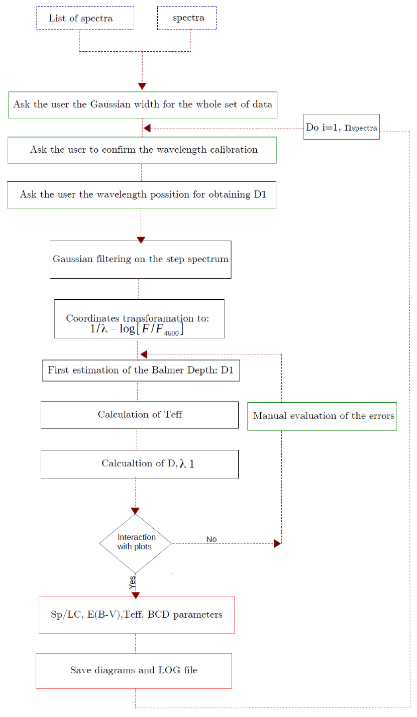
Figure 4: Simplified block diagram of the spectral analysis pipeline based on the BCD classification system presented in this work.

The output of the program is a log file containing the parameters calculated for each spectrum: name, BCD$(D,\lambda_{1})$, $T_{\rm eff}$, spectral type and luminosity class, $\Phi_{b}$, $\Phi_{b}^{0}$, $E(B-V)$ and M_V.

3 Observations and selection of the data.

3.1 IPHAS bright sample with FLWO/FAST

Follow-up spectroscopy of the emission line objects photometrically detected by IPHAS (Witham et al. 2008) was performed during the years 2005 to 2012 at the 1.5m Fred Laurence Whipple Observatory (FLWO) Tillinghast telescope on Mount Hopkins in Arizona, using the FAST spectrograph (Fabricant et al. 1998). The data were taken with the 300 lines $mm^{-1}$ grating, and a projected slit width of 3”. The data span a wavelength range from 3500 to $7500\ \AA$ at a spectral resolution of $\Delta\lambda\simeq 6\ \AA$.

The data were processed at the Telescope Data Center at the Smithsonian Astrophysical Observatory. The spectra were delivered without flux calibration. As explained in Sect. 2, the BCD method requires at least an accurate relative flux calibration, especially in the blue and near ultraviolet part of the spectrum, around the Balmer discontinuity. This spectral region is very hard to observe in a flux-calibrated way, due to the weakness of incandescent flat field calibration lamps, CCD efficiency and optical coating properties. For this reason we took special care in performing the flux calibration.

For each different night we selected calibration spectra from the FAST archive, to ensure that all spectra were calibrated with flux standards observed the same night. The calibration has been done using standard image reduction and analysis facility (IRAF) routines.

For 31 stars we have two spectra obtained at different epochs, and for one more three spectra. In Appendix B we present overplots of the different spectra obtained for each star and a detailed discussion on the reliability of the relative flux calibrations and the spectral parameters derived from them.

We estimate the mean error of the flux calibration as the difference between the individual values of the flux divided by the mean value. The mean error in the flux of the calibrated and normalised spectra amounts to 5.1$\pm$4.5% at $4000\ \AA$, and to 15$\pm$14% at $3600\ \AA$. The last value in the ultraviolet continuum is significantly larger, as expected. However, as explained in Sect. 2.1, to obtain the lower limit of the Balmer discontinuity of the CBe stars we don’t use the extrapolated ultraviolet continuum, but instead the bottom of the higher Balmer lines. Hence, even large errors in the flux calibration short of the Balmer discontinuity, which eventually could lead to an inaccurate determination of the slope or the position of the Balmer continuum, will not have any impact in the determination of the CBe stars physical parameters used through this work.

The mean difference between the measured $D$ and $\lambda_{1}$ parameters from different spectra of the same star are 0.032 dex and $7.3\AA$ respectively. These differences are of the same order as the ranges in $D$ and $\lambda_{1}$ spanned by one spectral subtype and one luminosity class respectively, as can be seen in Fig. 10 of Zorec et al. (2009).

For this work we selected the sources with spectral features characteristic of OB-type stars. Among them we selected the spectra which have S/N $\geq 30$ around the Balmer discontinuity ($\sim 3700\ \AA$), where the BCD parameters are measured. Finally, we rejected the spectra in which the continuum around the BD is not well defined. This rejection was applied automatically each time that the $\chi^{2}$ of a parabolic fit to the pseudo-continuum drawn in the BD region is larger than $3\sigma$ as compared to the average of fits obtained for the entire stellar sample. We considered that in those cases we could not derive a reliable $\lambda_{1}$ parameter.

We examined an initial sample sample of 612 FAST spectra in the Perseus Arm region. After rejecting the spectra whose characteristics did not correspond to an OB-type star, and those not meeting the criteria presented in the previous paragraph, we kept a final sample of 257 spectra for further analysis.

3.2 INT and NOT spectra

Mid-resolution (2-4 Å) and high S/N (30-100 at 3700 Å) spectra of 67 CBe stars were obtained at the Roque de los Muchachos Observatory in La Palma, Canary Islands, Spain. The telescopes and instruments used were the Isaac Newton Telescope (INT) equipped with the Intermediate Dispersion Spectrograph (IDS), and the Nordic Optical Telescope (NOT), using the Andalucía Faint Object Spectrograph and Camera (ALFOSC). A sample of spectrophotometric standard stars, for relative flux calibration, and MK standard stars, were also observed. A complete description of this data sample is given in Sect. 2.3 of Raddi et al. (2013).

These spectra have already been analysed by Raddi et al. (2013). In this work we will use them in the procedure to determine the value of $G$, the width of the gaussian filter required for the FLWO/FAST spectra, as described in the next subsection, and to compare the results of our analysis with those obtained by Raddi et al. (2013) via energy distribution fitting to appropriate model atmospheres.

3.3 Gaussian filtering

For every dataset, with different resolution, we must find the appropriate gaussian width with which to convolve the spectra in order to achieve the desired BCD resolution. The best way of doing this is to observe BCD standard stars with the same instrumental configuration as the programme stars. A list of BCD standards, that is, a sample of stars for which standard values of the $D$ and $\lambda_{1}$ parameters are know, is given by Zorec & Briot (1991).

No BCD standards were observed with the FAST spectrograph, and only two were obtained at the INT and two more at the NOT. In order to determine the value of $G$ (Eq. 2) and correct the resolution for all spectra we take the following steps:

1. As a starting point we used the INT and NOT spectra of the stars for which the standard $D$ and $\lambda_{1}$ are known. For each star we computed the BCD parameters using Gaussian filters of different width, and compared the obtained values with the standard ones. The best agreement for each star was obtained with the Gaussian widths presented in Table 1.

2. We obtained the BCD parameters of all MK standard stars observed with the INT and NOT, using the widths in Table 1. From the BCD parameters we obtained the spectral types and luminosity classes, and compared them with the standard MK ones. This comparison is presented in Table 2. The agreement between the MK and BCD classification is fairly good, within two spectral subtypes and one luminosity class for most of the stars. When comparing the classification of stars in both systems, we have to keep in mind that the MK system assigns discrete spectral types, where each encompasses comparatively large intervals of ($D,\lambda_{1}$) parameters. Obvious differences can then appear when interpreting continuous runs of BCD parameters with discrete MK assignments.

   From the above procedure, we find $G=$ 4.8, 4.0 and 3.5$\ \AA$ as the widths of the Gaussian filters to reduce the resolution of the INT (with two different instrumental configurations) and NOT spectra, respectively. We subsequently applied Gaussian filters of these widths to the whole sample of INT and NOT spectra, and computed the BCD parameters for all of them.

3. The final step is to set the resolution for the FAST spectra. The procedure is described graphically in Fig. 5. We convolved the FAST spectra, one by one, starting from a Gaussian width of 1.5$\ \AA$ up to 8$\ \AA$, with a 0.5$\ \AA$ step. For all the stars in common between the INT/NOT and FAST samples we plot the difference $\mid\lambda_{1,INT/NOT}-\lambda_{1,FAST}\mid$ versus the Gaussian width. The minimum difference is found at $G=4.25\ \AA$, and we assume this value to be the Gaussian width, $G$, with which to convolve all the FAST spectra prior to the determination of the BCD parameters from them.

Table 1: BCD standard stars observed with the INT and NOT telescopes. Columns 4, 5 and 6 are the standard BCD spectral type and $D$ and $\lambda_{1}$ parameters respectively, from Zorec & Briot (1991). The different $\Delta\lambda$ and dispersion values for the two stars observed at the INT are due to different instrumental configurations. The last column lists the width of the Gaussian filter used to reproduce the standard BCD parameters from each spectra.

NAME	Telescope	Sp/LCMK	Sp/LCBCD	$\lambda_{1}(\AA)$	$D(dex)$	$\Delta\lambda(\AA)$	Disp.$(\AA/pix)$	$G(\AA)$
HR 533	INT	B2 V	B2 V	65	0.144	4	1.85	4.8
HR 1122	NOT	B5 III	B5-6 III	42	0.286	2	0.72	3.5
HR 2347	NOT	B9 V	B9 V	64	0.422	2	0.72	3.5
HR 2461	INT	B8 III	B7 III	41	0.340	3	1.40	4.0

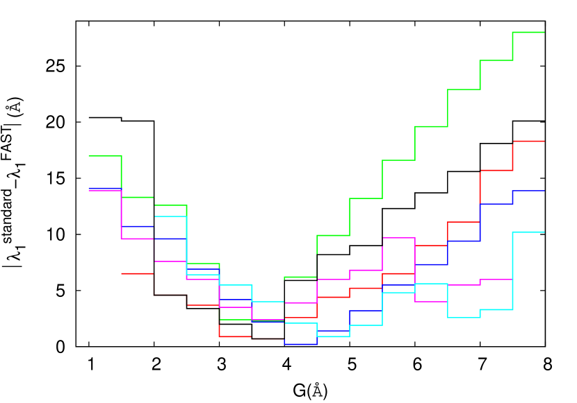
Figure 5: Differences in the $\lambda_{1}$ parameter obtained with the INT/NOT spectra and the FAST spectra convolved with different Gaussian widths ranging from 1.5 to 8$\ \AA$, at steps of 0.5$\ \AA$, for a subset of the stars in common between the two samples. Each colour represents a spectrum and the minimum of the $\Delta\lambda_{1}$ difference corresponds to the convolution that best fits the INT/NOT spectrum.

Table 2: Sample of 23 MK standard stars observed with the INT and NOT telescopes, covering almost all the B sub-types. We present the measured BCD parameters and the comparison between the standard MK type and the obtained BCD spectral classification.

NAME	Telescope	Sp/LCMK	Sp/LCBCD	$\lambda_{1}(\AA)$	$D_{uv}(dex)$	$D_{B.l.}(dex)$	$\mid D_{uv}-D_{B.l.}\mid$
HR 533	INT	B2 V	B2 V	79.4	0.162	0.149	0.013
HR 927	INT	B8 V	B7-8 V	54.3	0.346	0.345	0.001
HR 1122	NOT	B5 III	B5-6 III	36.1	0.236	0.237	0.001
HR 1399	INT	B5-6 V	B6 V	68.5	0.287	0.295	0.008
HR 1497	INT	B3 V	B7-8 V	77.0	0.294	0.297	0.003
HR 1576	INT	B9 V	B7 V	67.9	0.283	0.288	0.005
HR 1595	NOT	B2 V	B1 V	63.6	0.126	0.116	0.010
HR 1760	INT	A3V	¿A2	74.9	0.545	0.528	0.017
HR 1808	NOT	B5 V	B4 V	62.1	0.260	0.248	0.012
HR 1820	NOT	B2 V	B3 V	60.3	0.189	0.193	0.004
HR 1860	NOT	B6 V	B6 V	60.5	0.317	0.301	0.016
HR 1863	NOT	B2.5 V	B4 V	69.0	0.222	0.210	0.012
HR 1892	NOT	B1 V	B0 V	61.4	0.104	0.105	0.001
HR 2010	NOT	B9 IV	A0-1 V	65.7	0.483	0.464	0.019
HR 2116	NOT	B8 V	B7-8 V	62.7	0.355	0.340	0.015
HR 2161	NOT	B3 V	B3 V	64.4	0.205	0.213	0.008
HR 2344	INT	B2 V	B3 IV	54.0	0.183	0.182	0.001
HR 2347	NOT	B9 V	A0 V	66.6	0.473	0.453	0.020
HR 2461	INT	B8 III	B7-8 IV	45.4	0.349	0.351	0.002
HR 2490	NOT	B3 IV	B3 IV	51.6	0.242	0.227	0.015
HR 2840	INT	B6 IV	B7 IV	47.7	0.336	0.351	0.015
HR 7996	INT	B3 III	B3-4 IV	48.9	0.270	0.252	0.018
HR 8403	INT	B5 III	B5 V	54.3	0.331	0.313	0.018

4 Evaluation of the procedure

We now validate the described procedure, by comparing our results with results from the literature obtained for the same stars with different astrophysical techniques. For this comparison, we used the results obtained from spectroscopic data analysis by Raddi et al. (2013), and from Strömgren photometry calibration of data presented by Fabregat & Capilla (2005) and Monguió et al. (2013).

4.1 Validation against previous spectroscopic analyses

Raddi et al. (2013) studied a group of 67 candidate CBe stars in the region of the Perseus Arm, by analysing the mid resolution spectra obtained with the INT and NOT telescopes at La Palma described in Sect. 3.2. They determined their spectral types and measured their colour excess via spectral energy distribution fitting to appropriate model atmospheres in the blue part of the spectrum (3800-5000 Å).

For this comparison we use 35 spectra that meet the selection criteria described in Sect. 3.1. The results are presented in Table 3. To provide an additional element of comparison, in Table 3 we also present spectral types and luminosity classes obtained from the INT/NOT spectra by means of the standard MK classification procedures, using only the strength and widths of the spectral lines, and the ratios between lines, such as temperature and luminosity criteria, as described for example by Gray & Corbally (2009). In the last two columns we present the $E(B-V)$ obtained from the measured BCD parameters by means of Eq.1, and the absolute magnitudes in the scale defined by Zorec & Briot (1991). We estimate a mean error of 0.05 mag. for the $E(B-V)$ determination, obtained from the standard propagation of the errors through Eq. 1, considering the characteristic uncertainties of the BCD parameters involved. The mean uncertainty of the $M_{V}$ values amounts to 0.15 mag. (Zorec & Briot 1991).

From Table 3 we can see a general good agreement within the three classification systems. When comparing our results with those of Raddi et al. (2013) we find that 29 of the 35 stars agree within one or two spectral subtypes. In the remaining six stars, however, there are large differences. Better agreement, with differences not larger than two sub-spectral types, is found between the BCD results and the MK classification applied to the same spectra.

In Fig. 6 we present the comparison between the $E(B-V)$ obtained by Raddi et al. (2013) and our procedure. A mean error of 0.05 mag. for our determination of the $E(B-V)$ is assumed, as stated above. For the values of Raddi et al. (2013) we used the errors quoted by these authors. There is a good agreement between the two sets of data, with a mean difference of 0.04$\pm$0.15 mag.

Table 3: BCD parameters and classification of 35 IPHAS CBe stars with INT/NOT spectroscopy, and comparison with MK classification and spectral classification given by Raddi et al. (2013).

NAME	D (dex)	$\lambda_{1}(\AA)$	$\Phi_{b}$	$\Phi_{b}^{0}$	Sp/LCBCD	Sp/LCMK	Raddi et al.	$E(B-V)$	$M_{V}$
$J002441.73+642137.5$	0.291	36.5	2.85	0.80	B5-6III	B5III	B5III	1.38	-1.9
$J002926.93+630450.2$	0.355	72.3	1.51	0.85	B9V	B5-8V	B7V	0.44	1.0
$J004014.89+651644.0$	0.174	79.4	2.26	0.73	B3V	B2-3V	B2V	1.03	-1.5
$J005029.25+653330.8$	0.280	53.5	2.41	0.78	B5-6V	B3-4V	B7IV	1.10	-0.8
$J005436.84+630549.9$	0.195	63.3	2.10	0.73	B3V	B3V	B2-3V	0.92	-1.4
$J005611.62+630350.5$	0.280	69.9	1.53	0.79	B7V	B5-6V	B5V	0.50	-0.1
$J005619.50+625824.0$	0.288	70.2	1.07	0.80	B7V	B3-5V	B5V	0.18	-0.1
$J010707.68+625117.0$	0.291	60.8	2.40	0.79	B5V	B6-7Ia	B5V	1.09	-0.1
$J012405.42+660059.9$	0.246	54.8	1.94	0.76	B4V	B2-3V	B6IV	0.79	-1.0
$J012751.29+655104.0$	0.201	63.5	2.02	0.73	B3V	B3V	B7V	0.87	-1.3
$J014458.14+633244.0$	0.346	63.9	1.92	0.82	B7-8V	B3-4V	B7IV	0.74	0.6
$J014620.44+644802.5$	0.315	54.8	2.02	0.80	B6V	B5V	B7V	0.82	-0.4
$J014905.18+624912.3$	0.111	34.5	2.98	0.70	B2Ib	B2IV-III	B3IV	1.54	-5.6
$J015037.67+644446.9$	0.203	64.1	1.87	0.73	B3-4V	B3-5V	B4V	0.77	-1.1
$J015246.27+630315.0$	0.403	55.9	2.02	0.86	B9V	B8-9V	B8-9III	0.78	0.1
$J015613.22+635623.8$	0.165	68.8	1.64	0.72	B2V	B2V	B3V	0.62	-2.0
$J015918.32+654955.8$	0.321	69.0	2.22	0.85	B8V	B7-8V	B6IV	0.92	0.5
$J015922.53+635829.3$	0.234	57.1	1.91	0.75	B4V	B2-3V	B2-3V	0.78	-0.9
$J022337.05+601602.8$	0.185	52.9	2.26	0.73	B3-4IV	B3-4V	B7IV	1.03	-2.2
$J023031.39+594127.1$	0.268	50.0	1.95	0.77	B5-6V	B6-7V	B9V	0.79	-1.0
$J023404.70+605914.4$	0.184	60.5	2.71	0.73	B3-4V	B2V	B3IV	1.34	-1.5
$J023642.66+614714.9$	0.209	47.2	1.82	0.75	B3-4IV	B1-3V	B5V	0.72	-2.0
$J023744.52+605352.8$	0.142	43.6	2.52	0.70	B2III	-	B8	1.23	-3.7
$J024054.96+630009.7$	0.214	50.3	1.99	0.74	B3-4IV	B1-3V	B6	0.84	-1.6
$J024146.74+602532.2$	0.176	52.4	2.37	0.72	B2IV	B3III	B7V	1.11	-2.2
$J024159.21+600106.0$	0.197	57.6	2.18	0.73	B3-4V	B5V	B5V	0.98	-1.6
$J024317.68+603205.5$	0.120	44.2	2.26	0.70	B1III	B1.5-2III	B7V	1.05	-4.3
$J024504.86+612502.0$	0.257	43.4	2.09	0.78	B5-6IV	B6	B7IV	0.88	-1.8
$J024618.12+613514.7$	0.171	59.8	1.79	0.72	B2V	B2V	B3V	0.72	-1.9
$J025016.66+624435.6$	0.345	44.4	1.77	0.83	B7-8IV	B8-9V	B8-9III	0.63	-0.9
$J025059.14+615648.7$	0.147	62.7	1.76	0.70	B2V	B3V	B3-4V	0.71	-1.9
$J025233.25+615902.2$	0.244	40.7	1.83	0.77	B5-6III	B4V	B7V	0.71	-2.1
$J025448.85+605832.1$	0.296	59.5	1.97	0.79	B5-6V	B6-7V	B6V	0.79	-0.2
$J025610.40+580629.6$	0.161	55.2	2.04	0.71	B2V	B3-4V	B5V	0.90	-2.4
$J025700.49+575742.8$	0.152	47.1	2.24	0.71	B2III	B3-4V	B4V	1.03	-3.2

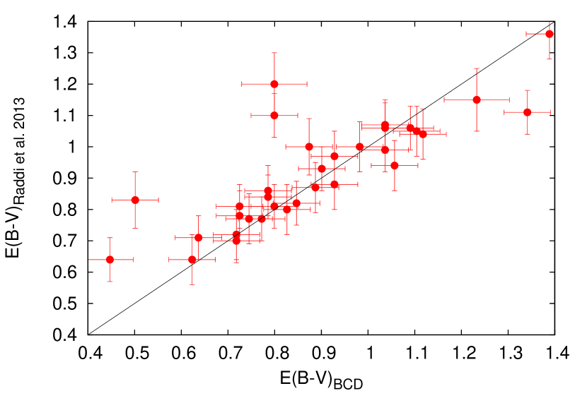
Figure 6: Comparison between the colour excesses obtained from the FAST spectra with the procedure described in this work and the values given by Raddi et al. (2013).

4.2 Validation with $uvby\beta$ photometry

Monguió et al. (2013) present a catalogue of $uvby\beta$ Strömgren-Crawford photometry for 35974 stars in the galactic anticentre direction. Thirteen classical Be stars for which we have FLWO/FAST spectroscopy have photometric data in this catalogue. In addition, two more CBe stars in the area of the galactic open cluster NGC 663, with available spectroscopy, have $uvby\beta$ photometry published by Fabregat & Capilla (2005).

For these stars we have obtained the interstellar reddening, spectral classification and absolute magnitude, using the $uvby\beta$ photometry calibrations given by Crawford (1978), Balona & Shobbrook (1984) and Moon (1986). We have followed the procedures described by Fabregat & Torrejón (1998) to apply the above calibrations to CBe stars, for which the circumstellar emission in the Balmer and Paschen continua and in the H$\beta$ line have large effects on the photometric indices.

In Table 4 we compare the results from the $uvby\beta$ photometry analysis with those obtained with the BCD techniques described in the previous sections. The differences in the spectral types between the two methods is within $\pm$1 subtype, as was the case between the BCD and MK classification systems. Regarding the luminosity class, we must note that the Strömgren photometry calibrations discriminate only between classes V and III, while the BCD procedures allow a more precise separation of classes V, IV and III.

In Fig. 7 we compare the values of $E(B-V)$ obtained with the BCD and Strömgren photometry techniques. For our determination we consider an error of 0.05 mag. as in the previous subsection. For the $uvby\beta$ calibration we use the error of 0.03 mag. quoted in Fabregat & Torrejón (1998). The agreement is very good, with a mean difference of =0.00$\pm$0.10 mag. In both the $uvby\beta$ calibrations and the BCD system the intrinsic colours of the stars are determined mainly from the depth of the Balmer discontinuity, measured through the $c_{1}$ index in the $uvby$ photometric system and through the $D$ parameter in the BCD system. Both determinations are consistent and lead to similar results.

Table 4: Comparison between the spectral classification and physical parameters obtained for 15 CBe stars and those obtained from Strömgren-Crawford photometry calibrations.

NAME	$D(dex)$	$\lambda_{1}(\AA)$	Sp/LCBCD	Sp/LCuvbyβ	$E(B-V)_{\rm BCD}$	$E(B-V)_{uvby\beta}$	$M_{V,BCD}$	$M_{V,uvby\beta}$
$J014602.11+611502.2$	0.191	67.2	B4V	B5-6V	0.917	1.113	$-0.3$	$-0.5$
$J014624.42+611037.3$	0.225	68.2	B5V	B5III	0.758	0.774	$-0.7$	$-2.3$
$J053237.14+260107.3$	0.290	47.9	B5-6V	B4V	0.917	0.990	$-1.4$	$-1.6$
$J053513.10+295912.4$	0.246	31.8	B3-4III	B3III	1.168	1.074	$-2.7$	$-2.5$
$J053554.13+295756.4$	0.221	77.9	B5V	B5V	1.362	1.290	$-1.4$	$-0.8$
$J053654.85+301757.8$	0.273	66.1	B5-6V	B5V	0.870	0.953	$-0.2$	$-0.4$
$J054033.87+274552.4$	0.398	65.4	B8V	B8V	0.619	0.758	0.5	0.2
$J054115.07+274803.2$	0.139	68.4	B2V	B3V	0.997	1.000	$-1.7$	$-0.7$
$J054159.24+274038.1$	0.254	74.6	B5-6V	B5V	0.774	0.710	$-0.4$	$-0.4$
$J054200.54+304956.6$	0.355	44.4	B7IV	B7V	0.599	0.743	$-0.0$	$-0.1$
$J054450.31+290754.5$	0.319	68.7	B7V	B7V	0.568	0.510	0.2	0.0
$J054603.64+272729.5$	0.211	48.9	B3IV	B2.5V	0.973	0.963	$-1.1$	$-1.9$
$J054837.64+281710.3$	0.179	63.4	B3V	B2V	0.945	0.843	$-1.4$	$-0.9$
$J054848.26+283547.8$	0.159	60.7	B2V	B1.5-2V	1.038	0.899	$-1.5$	$-2.2$
$J054937.88+281123.3$	0.329	70.3	B7V	B8V	0.520	0.438	0.2	0.2

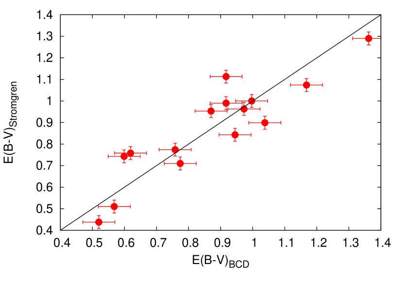
Figure 7: Comparison between the colour excesses obtained from the FAST spectra with the procedure described in this work and those obtained with Strömgren photometry techniques.

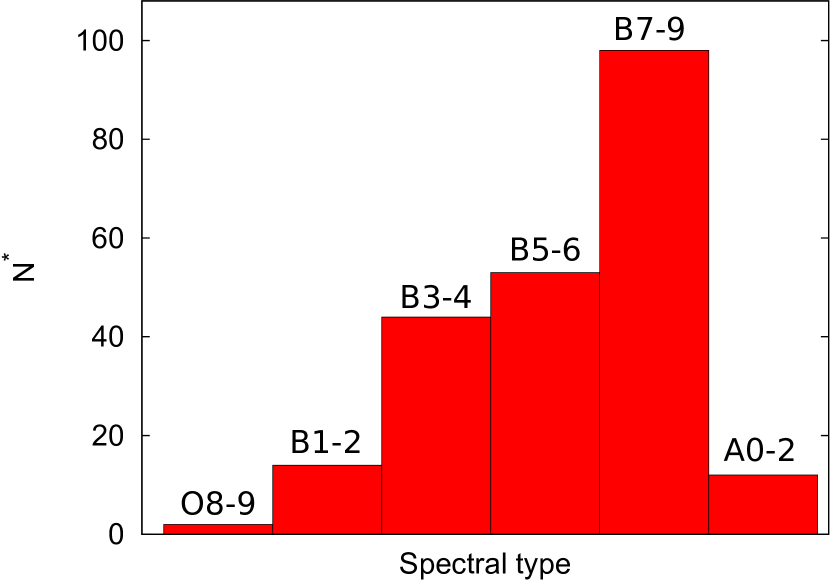
Figure 8: Histogram distribution of the spectral types.

5 Analysis of the Perseus Arm area.

As a further evaluation of our procedure, in this section we present the analysis of a sample of IPHAS follow-up spectra obtained with the FLWO/FAST spectrograph. We have selected the stars located in the Perseus arm region ($-1^{o}<b<4^{o}$, $120^{o}<l<140^{o}$). The population of CBe stars in this area has been investigated by Raddi et al. (2013), who analysed the INT and NOT spectra described in Sect. 3.2, and by Raddi et al. (2015) also using a sample of FAST spectra. In both papers the spectral classification was performed by comparison with standard templates, complemented with the application of standard procedures of the MK classification system. Both works stress the difficulty of assigning luminosity classes, due to the fact that the profiles of the Balmer lines, which provide the main luminosity indicators in the considered spectral range, are contaminated by the circumstellar emission characteristic of CBe stars.

In the BCD system, luminosities are derived from the $\lambda_{1}$ parameter, which is not affected by emission. As distance determination with the spectroscopic parallax technique heavily relies on the luminosity class of the objects, it is worthwhile to reproduce the above studies with reddenings and distances computed with the techniques described in this work, in order to compare the results.

Our analysis was done with 257 FAST spectra of 224 stars, that meet the criteria presented in Sect. 3.1. From each spectrum we determined the BCD ($D,\lambda_{1}$) parameters, the effective temperature, spectral type and luminosity class, interstellar and circumstellar colour excesses, absolute magnitude and distance. Results are presented in Tables 5 and 6. It took on average 2-3 minutes of work to analyse each star by means of our semi-automatic procedure.

We estimate the internal relative error in the determination of the effective temperature and distance as the difference between the individual values obtained from different spectra of the same star divided by the mean value. The mean errors measured in this way amount to 8% in $T_{\rm eff}$ and 24% in distance.

Eighteen stars, representing 8% of the sample, display the H$\alpha$ line in absorption. Since all the observed stars have been selected from a list of photometrically detected emission line stars (Witham et al. 2008), this figure can be considered as a measure of the false detection percentage of the photometric method. It should be noted, however, that the Be phenomenon is variable, and for some stars the lack of H$\alpha$ emission may be due to a phase transition from emission to absorption in the interval between the acquisition of the photometric and spectroscopic data. The above false detection figure must be considered as an upper limit.

Regarding the spectral classification, we found all sub-types from O8$-$9 up to A2. We found one Oe star, #66, with type O8$-$9IVe. The presence of visible He II lines in its spectrum confirms this classification. In Fig. 8 we present the histogram of the CBe star sample distribution as a function of the spectral types.

The spatial distribution found for the CBe star sample is presented in Fig. 9, where the 224 stars with distances listed in Table 6 are plotted. For stars with more than one spectrum we used the mean value of the distance determinations. The locations of the Perseus and Outer Galactic arms are marked with dotted lines, following the range of distances given by Russeil et al. (2007). Green represents the Perseus Arm at $\sim 2-3.5$ kpc. and blue the Outer Arm at $\sim 6-7$ kpc. The distribution of the stars does not present an apparent clustering in or around these two structures. Instead, they appear scattered along the two arms and the space in between, with some stars spread along larger distances, beyond the expected location of the Outer Arm. In Fig. 10 we present an histogram of the measured distances.These results are consistent with the findings of Raddi et al. (2013).

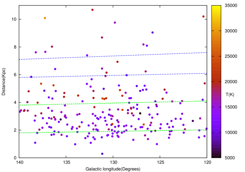
Figure 9: The distribution of the CBe stars distances as a function of the Galactic longitude. The green and blue dashed lines mark the expected positions of the Perseus and Outer Galactic arms, respectively. Five stars are at distances too long to appear in the diagram. The colour bar at the right-hand side represents the effective temperature of the stars.

For ten stars we found distances in excess of 9 kpc., well beyond the expected location of the Outer Galactic Arm. Five of them have distances larger than 11 kpc and hence they are out of the scale of Fig. 9. These distances in some cases can be due to large errors in the absolute magnitude or the spectral classification of the stars. A detailed discussion on the uncertainties and possible biasses in distance determination based on absolute magnitudes was given in Raddi et al. (2013). We are, however, studying in detail, for a future work a few stars in which the large distance seems to be consistently derived from high signal to noise spectra, in order to use them as tracers of the stellar population in the outskirts of the galactic plane.

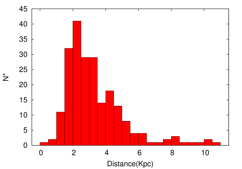
Figure 10: Histogram distribution of the distances.

6 Conclusions

This work is the first part of a larger project to study the whole population of CBe stars photometrically detected by the IPHAS survey, and use them as galactic structure tracers. The study will be based on the analysis of follow-up spectroscopy obtained at the FLWO telescope with the FAST spectrograph.

In this paper we have presented the method devised to obtain the spectral classification and the astrophysical parameters of the stars from the FLWO/FAST spectra, using the semi-automatic procedure we developed based on the BCD (Barbier-Chalonge-Divan) spectrophotometric system.

We have validated the method by comparing its results for two samples of CBe stars with independent results for the same stars obtained with different astrophysical techniques. In particular, we compared our results with those obtained with spectral template fitting and MK classification system standard techniques for one of the samples, and with Strömgren photometry standard calibrations for the other. In both cases we obtained a general good agreement in the spectral classification, within two spectral subtypes and one luminosity class for most of the stars. We have also compared our results on the interstellar extinction with those of the two samples referred to above, obtaining a good agreement in both cases.

We have also analysed a sample of CBe stars in the direction of the Perseus Arm ($-1^{o}<b<4^{o}$, $120^{o}<l<140^{o}$). We didn’t find any significant clustering of stars at the expected distances of the Perseus and Outer Arms. Even with over three times the number of stars considered by Raddi et al. (2013) we obtain the same negative result, indicating that the errors involved in the spectroscopic parallax and absolute magnitude determination blur any hint of Galactic spiral structure, if indeed the CBe stars trace it.

Table 5: Photometric $r$ magnitudes, H$\alpha$EW, BCD parameters, effective temperatures and spectral classification for the stars studied in this work. The parameters of stars with multiple spectra have been measured from each individual spectrum. They appear as multiple entries, with the same correlative number in the first column.

#	IPHAS NAME	$l$(deg)	$b$(deg)	$r$(mag)	H$\alpha$EW(Å)	$D$(dex)	$\lambda_{1}(\AA)$	$T_{\rm eff}(K)$	SpT/LC
1	J002540.04+623203.2	119.9	$-$0.18	14.46	$-$11.18	0.318	58.4	13186	B7$-$8V
2	J002754.61+603001.4	120.0	$-$2.23	13.66	$-$11.52	0.345	56.9	12380	B7$-$8 V
3	J002758.97+622906.1	120.2	$-$0.26	15.03	$-$16.39	0.206	59.4	18966	B3$-$4V
4	J002843.24+615216.2	120.2	$-$0.88	14.38	$-$14.33	0.294	65.5	13778	B7 V
5	J003000.79+612238.8	120.3	$-$1.38	14.24	$-$11.72	0.155	44.6	21195	B2 III
6	J003025.04+645500.0	120.7	2.13	15.95	$-$28.07	0.086	52.6	29473	B1 IV
7	J003055.94+610048.8	120.4	$-$1.75	15.39	$-$9.64	0.376	49.9	11980	B7$-$8 IV
8	J003210.31+623929.2	120.7	$-$0.13	13.39	$-$20.15	0.245	64.9	16295	B3$-$4 V
9	J003351.33+613743.1	120.8	$-$1.17	13.17	$-$5.10	0.386	63.9	11576	B9 V
10	J003421.40+601218.1	120.8	$-$2.59	14.21	$-$12.50	0.313	63.6	13091	B7$-$8 V
11	J003952.40+601719.5	121.4	$-$2.55	15.45	$-$14.98	0.554	62.2	6984	A0$-$1 IV
12	J004353.19+595641.6	121.9	$-$2.91	15.19	$-$38.97	0.103	86.5	27646	B1 V
13	J004620.80+622503.9	122.3	$-$0.44	13.18	$-$23.40	0.214	71.6	18352	B4 V
14	J004734.28+610833.6	122.4	$-$1.72	13.45	$-$2.01	0.388	70.4	11381	B9 V
15	J004741.54+624203.3	122.5	$-$0.16	14.15	$-$15.48	0.349	67.7	12063	B8 V
16	J004842.93+644411.1	122.6	1.86	14.74	$-$8.37	0.265	69.0	14819	B6 V
17	J004850.12+642533.7	122.6	1.55	15.64	$-$22.53	0.231	58.2	17261	B3$-$4V
18	J005011.87+635129.9	122.7	0.98	13.75	$-$26.21	0.296	76.9	13066	B7 V
19	J005032.31+623155.5	122.8	$-$0.33	15.43	$-$15.40	0.310	67.1	13021	B7 V
20	J005458.91+633913.2	123.3	0.78	13.90	$-$12.54	0.393	51.3	11670	B7$-$8 V
21	J005743.72+640235.6	123.6	1.17	14.18	$-$16.84	0.378	73.7	11474	B9 V
22	J005809.86+624412.9	123.7	$-$0.12	14.67	$-$26.30	0.246	69.9	16131	B5 V
23	J005859.29+632603.4	123.7	0.57	13.17	$-$37.62	0.298	63.8	13695	B5$-$6 V
23	J005859.29+632603.4	123.7	0.57	13.17	$-$33.55	0.329	71.7	12286	B8 V
24	J005926.64+651157.0	123.7	2.34	13.45	$-$22.53	0.319	60.5	13038	B7$-$8V
25	J010051.26+641327.3	123.9	1.37	13.61	$-$11.96	0.311	70.4	12775	B7 V
26	J010054.58+643729.6	123.9	1.77	13.02	$-$17.60	0.256	69.2	15376	B5 V
27	J010107.85+633227.0	124.0	0.68	13.84	$-$14.54	0.278	67.4	14329	B7 V
28	J010138.04+641349.9	124.0	1.38	13.32	$-$31.12	0.266	65.9	14895	B6 V
29	J010150.19+603917.9	124.2	$-$2.19	13.26	$-$3.59	0.340	63.3	12314	B7$-$8 V
30	J010232.39+602615.1	124.3	$-$2.40	14.33	$-$12.24	0.311	60.2	13365	B5$-$6 V
31	J010358.11+595310.9	124.5	$-$2.94	13.90	$-$22.03	0.197	78.1	19139	B3$-$4 V
32	J010551.90+602737.5	124.7	$-$2.36	13.57	$-$27.42	0.200	65.9	19329	B3$-$4 V
33	J010733.72+604206.8	124.9	$-$2.10	13.07	$-$18.13	0.276	69.0	14365	B6 V
34	J010841.17+615511.8	124.9	$-$0.88	13.72	$-$16.28	0.402	70.4	11165	A0$-$1 V
35	J010911.94+582207.9	125.2	$-$4.42	14.48	9.39	0.426	75.1	10579	A0$-$1 V
36	J011112.59+584912.7	125.4	$-$3.95	15.14	8.14	0.310	74.6	12550	B7$-$8 V
37	J011117.82+605958.2	125.3	$-$1.77	15.06	9.52	0.441	70.9	10415	A0$-$1 V
38	J011216.30+615051.2	125.3	$-$0.92	13.56	1.35	0.232	69.5	17172	B5 V
39	J011234.21+630432.5	125.3	0.30	12.64	$-$24.39	0.296	65.4	13688	B7 V
40	J011352.28+590144.6	125.8	$-$3.71	13.27	$-$20.21	0.274	75.2	14181	B7 V
41	J011402.43+625735.3	125.4	0.20	12.91	$-$23.16	0.217	78.0	18014	B5$-$6 V
42	J011520.26+585002.9	126.0	$-$3.89	13.02	$-$27.92	0.264	66.5	14958	B6 V
43	J011542.33+602558.4	125.9	$-$2.29	13.33	$-$39.65	0.352	70.0	11954	B9 V
44	J011556.37+584812.1	126.1	$-$3.91	13.48	$-$11.86	0.372	59.9	11886	B7$-$8V
45	J011720.92+634727.8	125.7	1.06	14.99	$-$75.07	0.476	25.6	9889	A0$-$1 II
46	J011735.90+580930.8	126.3	$-$4.53	15.70	$-$11.03	0.310	60.3	13397	B5$-$6 V
47	J011756.05+601019.7	126.2	$-$2.53	14.93	10.90	0.429	72.0	10621	A0$-$1 V
48	J011757.12+594045.9	126.2	$-$3.02	13.09	$-$18.67	0.244	60.3	16507	B3$-$4 V
49	J011824.08+583517.7	126.4	$-$4.09	15.34	6.60	0.407	67.2	11170	A0$-$1 V
50	J011858.17+583817.4	126.5	$-$4.04	15.43	4.77	0.217	79.8	17957	B5$-$6 V
51	J011918.18+642233.8	125.9	1.66	13.44	$-$41.30	0.225	70.6	17676	B5 V
52	J012049.08+580633.6	126.8	$-$4.54	15.04	11.41	0.421	78.8	10568	A0$-$1 V
53	J012127.39+602706.9	126.6	$-$2.20	15.57	7.83	0.343	64.6	12239	B7$-$8 V
54	J012350.55+585848.1	127.1	$-$3.62	15.23	17.01	0.362	74.2	11714	B7$-$8 V
55	J012358.07+652615.4	126.3	2.77	13.72	$-$16.94	0.301	66.1	13443	B7 V
56	J012416.80+633011.7	126.5	0.86	13.10	$-$12.68	0.233	69.2	17116	B5 V
56	J012416.80+633011.7	126.5	0.86	13.10	$-$13.07	0.231	74.5	17112	B5$-$6 V
57	J012417.10+592450.7	127.1	$-$3.19	15.37	9.62	0.450	69.2	10291	A0$-$1 V
58	J012430.74+622156.5	126.7	$-$0.26	16.69	$-$39.40	0.254	58.8	1597	B5$-$6V

Table 5. Continued…

#	IPHAS NAME	$l$(deg)	$b$(deg)	$r$(mag)	H$\alpha$EW(Å)	$D$(dex)	$\lambda_{1}(\AA)$	$T_{\rm eff}(K)$	SpT/LC
59	J012536.96+593053.0	127.2	$-$3.06	13.74	7.81	0.303	70.1	13123	B7 V
60	J012540.57+623025.7	126.8	$-$0.10	13.42	$-$24.40	0.278	79.4	13801	B5$-$6 V
61	J012611.30+585127.4	127.4	$-$3.71	15.54	9.05	0.355	74.5	11820	B7$-$8 V
62	J012634.69+641850.9	126.7	1.70	12.77	$-$17.65	0.136	69.0	25369	B1 V
63	J012657.63+591436.3	127.4	$-$3.31	15.52	5.21	0.450	70.3	10251	A0$-$1 V
64	J012745.08+625154.3	127.0	0.28	13.46	$-$18.13	0.403	69.4	11182	B9 V
65	J012821.12+635754.0	126.9	1.38	14.63	1.88	0.069	62.2	33482	O8$-$9 IV
66	J013104.42+602337.3	127.8	$-$2.10	14.26	$-$4.40	0.402	64.7	11295	B9 V
67	J013130.51+630914.4	127.4	0.63	15.08	$-$49.84	0.240	72.4	16468	B6$-$7V
68	J013213.92+623717.2	127.6	0.12	13.32	$-$9.97	0.257	68.8	15327	B5 V
68	J013213.92+623717.2	127.6	0.12	13.32	$-$11.13	0.270	67.9	14667	B6 V
69	J013244.08+595633.6	128.0	$-$2.51	14.35	$-$14.03	0.378	57.2	11824	B7$-$8 V
70	J013328.71+610759.4	127.9	$-$1.32	12.68	$-$23.86	0.209	68.3	18725	B4 V
71	J013402.88+611358.6	128.0	$-$1.21	12.92	$-$19.18	0.302	74.5	12914	B7$-$8 V
72	J013422.61+624459.7	127.8	0.28	12.92	$-$31.32	0.246	69.8	16130	B5 V
73	J013539.04+610341.6	128.2	$-$1.35	14.46	$-$23.80	0.279	67.4	14306	B7 V
74	J013706.99+585234.3	128.8	$-$3.47	13.47	$-$24.85	0.307	71.2	12876	B7 V
75	J013729.25+603806.2	128.5	$-$1.73	15.46	$-$9.88	0.316	74.1	12444	B7$-$8 V
76	J013739.40+613258.8	128.4	$-$0.82	14.31	$-$11.31	0.227	71.3	17533	B5 V
77	J013819.58+635306.0	128.0	1.48	12.98	$-$61.20	0.155	58.2	23018	B2 V
78	J013825.56+635008.5	128.0	1.43	13.96	$-$15.17	0.221	59.9	17965	B3$-$4V
79	J013920.80+654338.7	127.8	3.31	13.64	$-$14.93	0.337	65.8	12311	B8 V
80	J014146.63+581803.4	129.5	$-$3.92	15.11	$-$14.70	0.194	72.4	19560	B3 V
81	J014221.27+645836.1	128.2	2.63	15.24	$-$12.79	0.324	74.7	12292	B7$-$8 V
82	J014238.73+633753.1	128.5	1.32	13.18	$-$6.29	0.267	69.1	14753	B6 V
83	J014244.86+623056.2	128.8	0.23	13.22	$-$10.71	0.320	62.1	12925	B7$-$8V
84	J014322.19+640118.5	128.5	1.72	13.29	$-$20.99	0.280	74.3	13951	B7$-$8 V
85	J014323.30+595307.3	129.4	$-$2.33	13.69	$-$50.78	0.287	63.4	14165	B5$-$6 V
86	J014401.85+640124.5	128.6	1.73	15.49	$-$17.87	0.249	74.4	15613	B5$-$6 V
87	J014437.08+603458.0	129.4	$-$1.61	13.22	$-$35.85	0.243	70.5	16304	B5 V
88	J014452.24+604123.3	129.4	$-$1.50	13.88	$-$6.41	0.293	73.9	13360	B7$-$8 V
89	J014458.27+625245.8	128.9	0.63	13.35	$-$23.31	0.137	78.1	24504	B2 V
90	J014539.64+611259.1	129.4	$-$0.97	12.45	$-$21.60	0.202	67.0	19157	B3$-$4 V
91	J014552.19+660933.3	128.4	3.86	16.37	$-$22.87	0.454	82.3	9659	A0$-$1 V
92	J014602.11+611502.2	129.4	$-$0.92	13.75	$-$38.91	0.243	75.9	16126	B5 V
93	J014624.42+611037.3	129.5	$-$0.99	13.36	$-$4.11	0.278	74.2	14051	B7$-$8 V
94	J014659.63+611229.6	129.5	$-$0.94	13.23	$-$26.33	0.292	73.3	13443	B7$-$8 V
95	J014807.07+631613.2	129.2	1.09	13.54	$-$34.11	0.158	55.0	22559	B2 V
96	J014843.39+642854.4	129.0	2.29	13.74	$-$22.26	0.326	68.8	12398	B8 V
97	J015022.92+652743.2	129.0	3.28	13.79	$-$6.99	0.168	66.4	21798	B2 V
98	J015025.75+602245.2	130.1	$-$1.66	14.05	$-$11.10	0.364	69.1	11799	B9 V
99	J015105.68+611602.6	130.0	$-$0.77	13.71	$-$9.74	0.332	73.2	12202	B7$-$8 V
100	J015109.13+641421.8	129.3	2.11	15.71	$-$13.82	0.312	62.4	13199	B7$-$8V
101	J015123.63+600038.6	130.3	$-$1.99	12.76	$-$27.30	0.243	76.6	16067	B5$-$6 V
102	J015213.08+624813.6	129.8	0.74	13.04	$-$11.33	0.339	62.6	12359	B7$-$8 V
103	J015307.22+650110.4	129.3	2.92	13.97	$-$10.32	0.381	66.0	11605	B9 V
104	J015314.56+620241.5	130.1	0.03	12.89	$-$7.02	0.394	57.4	11563	B9 V
105	J015329.19+643128.1	129.5	2.45	13.98	$-$5.44	0.468	70.2	9768	A0$-$1 V
106	J015520.62+611752.8	130.5	$-$0.62	13.46	$-$17.91	0.361	70.0	11824	B9 V
107	J015538.88+600157.0	130.8	$-$1.84	14.31	$-$18.47	0.321	58.7	13037	B7$-$8V
108	J015627.82+612939.2	130.6	$-$0.4	12.70	$-$15.70	0.280	71.6	14075	B7 V
109	J015630.89+630307.5	130.2	1.10	13.27	$-$28.90	0.261	69.1	15022	B6 V
109	J015630.89+630307.5	130.2	1.10	13.27	$-$29.25	0.315	78.3	12309	B5$-$6 V
110	J015645.78+635259.6	130.0	1.91	13.11	$-$20.40	0.232	46.3	16988	B3$-$4 IV
110	J015645.78+635259.6	130.0	1.91	13.11	$-$19.93	0.222	69.2	17828	B4 V
111	J015650.51+645341.1	129.8	2.89	15.43	$-$19.97	0.254	46.3	16040	B5$-$6 IV
112	J015716.62+575205.7	131.6	$-$3.88	13.15	$-$11.84	0.282	62.7	14410	B5$-$6 V
113	J015804.46+653020.6	129.7	3.52	13.14	$-$8.98	0.301	56.6	13917	B5$-$6 V
114	J015809.04+615813.6	130.6	0.10	14.59	$-$21.84	0.196	50.5	19465	B3$-$4 IV
115	J015919.69+645053.4	130.0	2.92	12.78	$-$16.11	0.303	70.4	13099	B7 V

Table 5. Continued…

#	IPHAS NAME	$l$(deg)	$b$(deg)	$r$(mag)	H$\alpha$EW(Å)	$D$(dex)	$\lambda_{1}(\AA)$	$T_{\rm eff}(K)$	SpT/LC
116	J015939.01+643615.4	130.1	2.69	13.26	$-$18.10	0.282	50.5	14790	B5$-$6 V
116	J015939.01+643615.4	130.1	2.69	13.26	$-$21.62	0.279	61.6	14550	B5$-$6 V
117	J020037.84+652133.9	130.0	3.45	13.08	3.84	0.151	71.9	23301	B2 V
118	J020048.75+585835.1	131.7	$-$2.69	13.58	$-$13.89	0.375	68.3	11640	B9 V
118	J020048.75+585835.1	131.7	$-$2.69	13.58	$-$14.27	0.335	72.4	12174	B8 V
119	J020049.45+635943.9	130.4	2.14	13.91	$-$28.90	0.223	58.6	17824	B3$-$4V
120	J020056.02+575529.3	132.0	$-$3.70	14.99	$-$9.65	0.204	74.9	18827	B4 V
121	J020105.33+613403.0	131.1	$-$0.19	14.46	$-$36.57	0.130	74.1	25613	B1 V
122	J020109.65+641219.4	130.4	2.35	14.58	$-$8.10	0.394	74.7	11204	B9 V
123	J020136.00+613207.6	131.1	$-$0.20	13.14	$-$9.90	0.385	53.7	11779	B7$-$8 V
124	J020144.88+581929.8	132.0	$-$3.29	13.05	$-$8.18	0.188	78.3	19640	B3$-$4 V
124	J020144.88+581929.8	132.0	$-$3.29	13.05	$-$11.27	0.183	78.9	19860	B3$-$4 V
125	J020252.26+620926.0	131.1	0.43	15.21	$-$22.89	0.224	52.3	17564	B3$-$4 IV
126	J020325.84+584145.0	132.1	$-$2.87	15.42	$-$28.06	0.197	78.3	19138	B3$-$4 V
127	J020326.01+635943.1	130.7	2.21	14.40	$-$16.49	0.162	77.5	21809	B2 V
127	J020326.01+635943.1	130.7	2.21	14.40	$-$17.27	0.212	78.9	18231	B3$-$4 V
128	J020328.05+624334.0	131.0	0.99	13.73	$-$12.87	0.310	46.1	13872	B5$-$6 IV
129	J020343.87+581058.2	132.3	$-$3.35	12.84	$-$7.74	0.279	71.8	14102	B6 V
130	J020407.85+643122.2	130.6	2.74	13.94	$-$15.28	0.258	64.4	15492	B5$-$6 V
130	J020407.85+643122.2	130.6	2.74	13.94	$-$14.45	0.273	66.2	14601	B6 V
131	J020421.09+591708.1	132.1	$-$2.27	13.50	$-$13.07	0.260	67.0	15176	B6 V
132	J020422.15+595855.8	131.9	$-$1.60	13.42	$-$9.43	0.371	62.8	11830	B7$-$8 V
133	J020504.17+630216.1	131.1	1.34	15.07	$-$4.30	0.262	47.8	15684	B5$-$6 IV
134	J020547.47+641051.7	130.9	2.46	12.68	$-$10.88	0.160	54.8	22348	B2 IV
135	J020618.67+644945.1	130.7	3.10	14.88	$-$30.85	0.216	76.2	18072	B4 V
136	J020649.26+645826.9	130.7	3.26	14.49	$-$9.63	0.330	53.0	12952	B7$-$8 V
137	J020707.67+612422.7	131.8	$-$0.14	13.28	$-$11.88	0.279	58.7	14677	B5$-$6V
138	J020710.67+602546.5	132.1	$-$1.07	14.40	$-$16.84	0.260	59.5	15610	B5$-$6V
139	J020753.51+644148.9	130.9	3.02	15.91	$-$6.53	0.502	55.7	9520	A0$-$1 IV
140	J020826.27+625745.9	131.5	1.38	14.37	$-$18.27	0.377	45.9	12006	B7$-$8 IV
141	J020826.93+642241.5	131.1	2.74	12.59	$-$8.89	0.484	73.6	8738	A1 V
142	J020833.88+585547.6	132.7	$-$2.40	15.93	$-$10.54	0.294	62.3	13936	B5$-$6 V
143	J020859.72+635536.1	131.3	2.32	14.94	$-$9.61	0.332	66.8	12361	B8 V
144	J020917.87+613045.2	132.0	0.03	13.89	$-$17.24	0.253	56.6	16086	B3$-$4 V
145	J021057.06+624700.8	131.8	1.30	14.02	$-$5.66	0.354	55.9	12246	B7$-$8 V
146	J021128.86+634604.0	131.6	2.25	13.93	$-$12.12	0.339	65.0	12293	B8 V
147	J021210.42+623242.3	132.0	1.11	12.20	$-$18.76	0.284	70.2	13973	B7 V
148	J021310.78+572406.7	133.7	$-$3.73	13.20	$-$12.04	0.315	72.7	12516	B7$-$8 V
149	J021320.12+613003.1	132.5	0.16	12.89	$-$21.50	0.233	58.9	17154	B3$-$4V
150	J021336.53+601829.1	132.9	$-$0.95	13.75	$-$5.73	0.315	67.8	12751	B7 V
151	J021352.00+642520.3	131.6	2.96	15.03	$-$13.20	0.321	68.8	12513	B8 V
152	J021544.45+582456.8	133.7	$-$2.66	13.33	$-$17.56	0.285	67.4	14060	B7 V
153	J021744.41+644335.2	131.9	3.38	13.70	$-$19.02	0.197	52.7	19457	B3$-$4 V
153	J021744.41+644335.2	131.9	3.38	13.70	$-$25.31	0.238	46.6	16726	B3$-$4 IV
154	J022009.76+643605.9	132.2	3.35	15.65	$-$10.96	0.331	51.2	12982	B7$-$8 V
154	J022009.76+643605.9	132.2	3.35	15.65	$-$10.23	0.406	49.2	11470	B9 IV
155	J022025.02+600114.0	133.8	$-$0.95	13.31	5.99	0.288	69.6	13820	B7 V
156	J022045.25+631642.8	132.7	2.12	15.02	$-$18.80	0.320	61.1	12953	B7$-$8V
157	J022053.65+642835.6	132.3	3.25	15.91	$-$14.18	0.283	58.9	14519	B5$-$6V
158	J022100.28+635435.2	132.5	2.72	13.09	$-$10.63	0.402	56.7	11450	B9 V
159	J022343.45+603545.6	134.0	$-$0.27	12.94	$-$10.95	0.278	63.5	14530	B5$-$6 V
160	J022420.71+624842.7	133.3	1.82	13.43	$-$16.21	0.383	38.0	11851	B7$-$8 III
161	J022502.71+644947.7	132.6	3.74	13.26	$-$9.81	0.369	48.0	12126	B7$-$8 IV
161	J022502.71+644947.7	132.6	3.74	13.26	$-$8.85	0.334	60.1	12480	B7$-$8V
162	J022558.78+583626.1	134.9	$-$2.03	15.11	$-$21.23	0.364	78.6	11589	B9 V
163	J022823.86+631834.8	133.5	2.45	12.78	$-$28.41	0.188	70.6	19993	B3 V
164	J022913.58+633224.5	133.5	2.70	13.74	$-$14.74	0.230	57.3	17341	B3$-$4 V
164	J022913.58+633224.5	133.5	2.70	13.74	$-$11.56	0.191	65.6	19946	B3$-$4 V
165	J023003.21+643829.4	133.2	3.76	15.31	$-$18.01	0.315	55.3	13422	B5$-$6 V
166	J023150.04+604952.4	134.8	0.30	13.85	$-$53.87	0.394	76.0	11169	B9 V

Table 5. Continued…

#	IPHAS NAME	$l$(deg)	$b$(deg)	$r$(mag)	H$\alpha$EW(Å)	$D$(dex)	$\lambda_{1}(\AA)$	$T_{\rm eff}(K)$	SpT/LC
167	J023235.12+640522.8	133.7	3.35	13.52	$-$37.29	0.180	46.8	20188	B3$-$4 IV
168	J023410.30+612440.6	134.9	0.95	13.64	$-$92.45	0.336	80.0	11985	B8 V
169	J023411.99+595634.4	135.4	$-$0.40	13.13	$-$17.33	0.241	74.5	16334	B5$-$6 V
169	J023411.99+595634.4	135.4	$-$0.40	13.13	$-$16.63	0.241	69.0	16524	B5 V
170	J023758.12+634635.6	134.3	3.29	13.30	$-$8.86	0.388	63.0	11554	B9 V
170	J023758.12+634635.6	134.3	3.29	13.30	$-$9.42	0.435	55.5	10930	B9 V
171	J023809.91+620224.6	135.0	1.71	13.20	$-$14.26	0.244	51.6	16531	B3$-$4 IV
171	J023809.91+620224.6	135.0	1.71	13.20	$-$14.70	0.264	49.2	15580	B5$-$6 IV
172	J023841.80+640826.3	134.3	3.66	14.06	$-$10.80	0.263	61.8	15270	B5$-$6 V
172	J023841.80+640826.3	134.3	3.66	14.06	$-$11.13	0.326	53.5	13075	B7$-$8 V
173	J023923.67+604247.6	135.7	0.55	13.33	$-$24.97	0.319	61.8	12984	B7$-$8V
174	J023948.17+604505.1	135.7	0.61	13.26	$-$15.20	0.329	69.9	12321	B8 V
175	J023950.95+611829.1	135.5	1.12	13.95	$-$49.84	0.558	76.2	5065	A2
176	J024021.07+582834.0	136.7	$-$1.43	13.81	$-$6.15	0.395	57.5	11544	B9 V
177	J024132.66+550235.9	138.3	$-$4.50	13.22	$-$8.85	0.376	62.3	11773	B7$-$8V
178	J024146.73+602532.5	136.1	0.41	14.05	$-$34.38	0.230	57.8	17340	B3$-$4V
179	J024221.54+593716.4	136.5	$-$0.28	13.38	$-$14.61	0.447	51.2	10773	B9 IV
179	J024221.54+593716.4	136.5	$-$0.28	13.38	$-$14.06	0.387	58.0	11666	B9 V
180	J024317.67+603205.6	136.2	0.59	13.67	$-$36.70	0.218	60.4	18146	B3$-$4 V
181	J024332.09+632150.2	135.1	3.17	14.16	$-$18.06	0.280	59.4	14615	B5$-$6V
181	J024332.09+632150.2	135.1	3.17	14.16	$-$17.06	0.314	47.5	13701	B5$-$6 IV
181	J024332.09+632150.2	135.1	3.17	14.16	$-$17.42	0.284	61.9	14339	B5$-$6 V
182	J024504.86+612502.1	136.0	1.48	15.35	$-$15.31	0.299	56.6	13990	B5$-$6 V
183	J024519.12+633755.1	135.1	3.50	14.04	$-$35.64	0.205	69.0	18929	B4 V
183	J024519.12+633755.1	135.1	3.50	14.04	$-$35.91	0.178	54.3	20910	B2 IV
184	J024521.28+625416.2	135.4	2.84	13.59	$-$14.91	0.259	68.6	15190	B5 V
185	J024540.62+592151.1	137.0	$-$0.34	13.28	$-$23.31	0.272	62.9	14762	B5$-$6 V
185	J024540.62+592151.1	137.0	$-$0.34	13.28	$-$24.27	0.299	60.7	13816	B5$-$6 V
186	J024553.87+635414.7	135.1	3.77	14.21	$-$14.71	0.241	60.8	16675	B3$-$4 V
187	J024618.12+613514.8	136.1	1.70	15.70	$-$26.84	0.334	58.3	12564	B7$-$8V
188	J024735.56+615530.9	136.1	2.07	13.43	$-$19.76	0.275	49.8	15049	B5$-$6 IV
188	J024735.56+615530.9	136.1	2.07	13.43	$-$18.52	0.298	72.2	13248	B7 V
189	J024737.27+640509.3	135.2	4.02	14.24	$-$19.54	0.187	76.9	19748	B3 V
190	J024748.62+605750.5	136.5	1.21	13.95	$-$50.74	0.419	81.1	10533	A0$-$1 V
191	J024753.07+613405.8	136.3	1.76	14.37	$-$29.43	0.133	72.6	25441	B1 V
192	J024823.01+614728.1	136.2	1.99	12.91	$-$19.60	0.282	63.7	14368	B5$-$6 V
193	J024928.49+595248.5	137.2	0.32	13.37	$-$26.52	0.089	54.5	29771	B1 IV
194	J024940.66+621424.8	136.2	2.46	13.24	$-$20.52	0.320	79.9	12235	B9 V
195	J025059.16+615648.8	136.4	2.26	15.28	$-$30.51	0.191	89.7	18933	B4 V
196	J025102.24+615733.8	136.4	2.27	14.07	$-$45.41	0.206	47.7	18582	B3$-$4 IV
197	J025106.28+580120.6	138.2	$-$1.24	14.84	$-$16.49	0.232	60.1	17211	B3$-$4 V
198	J025130.43+621052.2	136.4	2.50	15.79	$-$38.26	0.372	64.0	11797	B7$-$8 V
199	J025136.03+601557.5	137.3	0.79	15.81	$-$16.90	0.447	83.5	9799	A0$-$1 V
200	J025200.23+621145.2	136.4	2.54	13.85	$-$16.26	0.310	60.5	13403	B5$-$6 V
201	J025324.54+614622.9	136.8	2.23	15.46	$-$20.73	0.353	68.3	11986	B9 V
202	J025700.51+575742.9	138.9	$-$0.94	14.26	$-$23.34	0.188	84.3	19329	B3$-$4 V
203	J025737.78+624703.4	136.8	3.36	14.77	$-$12.78	0.333	65.4	12388	B8 V
204	J025856.75+633557.7	136.5	4.15	13.48	$-$33.96	0.228	74.4	17411	B5$-$6 V
204	J025856.75+633557.7	136.5	4.15	13.48	$-$34.82	0.315	61.5	13135	B7$-$8V
205	J025904.88+621459.5	137.1	2.96	15.59	$-$6.29	0.247	79.5	15593	B5$-$6 V
206	J025905.15+605404.2	137.8	1.77	12.91	$-$45.34	0.214	72.4	18280	B4 V
207	J025935.04+603207.2	138.0	1.48	13.88	$-$18.73	0.394	67.3	11362	B9 V
207	J025935.04+603207.2	138.0	1.48	13.88	$-$18.96	0.343	62.5	12297	B7$-$8 V
208	J025950.85+582333.1	139.1	$-$0.38	14.05	$-$83.18	0.221	87.6	17596	B5 V
209	J025959.45+582929.5	139.0	$-$0.29	13.31	$-$14.69	0.214	45.8	17929	B3$-$4 IV
210	J030010.27+613223.2	137.6	2.40	13.73	$-$7.90	0.143	63.5	24599	B2 V
210	J030010.27+613223.2	137.6	2.40	13.73	$-$13.23	0.133	59.8	25623	B1 V
211	J030056.70+615940.8	137.5	2.84	13.04	2.51	0.288	68.4	13892	B7 V
211	J030056.70+615940.8	137.5	2.84	13.04	0.81	0.282	77.1	13739	B7 V
212	J030121.61+602856.6	138.2	1.54	13.89	$-$21.83	0.360	66.8	11923	B9 V

Table 5. Continued…

#	IPHAS NAME	$l$(deg)	$b$(deg)	$r$(mag)	H$\alpha$EW(Å)	$D$(dex)	$\lambda_{1}(\AA)$	$T_{\rm eff}(K)$	SpT/LC
213	J030124.02+610221.3	138.0	2.03	14.85	$-$29.58	0.174	73.2	21026	B2 V
214	J030144.21+632853.5	136.8	4.19	14.39	$-$7.81	0.268	57.1	15258	B5$-$6 V
214	J030144.21+632853.5	136.8	4.19	14.39	$-$7.89	0.272	61.8	14835	B5$-$6 V
215	J030317.45+583402.0	139.4	$-$0.01	14.57	$-$20.15	0.280	44.0	14877	B5$-$6 IV
216	J030331.33+585234.6	139.2	0.26	14.64	$-$8.18	0.111	35.5	20644	B2 Ib
217	J030332.31+623856.7	137.4	3.56	14.32	$-$8.93	0.356	50.9	12303	B7$-$8 V
217	J030332.31+623856.7	137.4	3.56	14.32	$-$8.98	0.393	59.1	11562	B9 V
218	J030422.01+574820.4	139.9	$-$0.61	14.40	$-$26.00	0.271	76.6	14260	B6 V
218	J030422.01+574820.4	139.9	$-$0.61	14.40	$-$24.15	0.246	80.0	15646	B5$-$6 V
219	J030423.32+622900.9	137.6	3.46	13.70	$-$22.53	0.216	59.4	18295	B3$-$4V
219	J030423.32+622900.9	137.6	3.46	13.70	$-$22.85	0.219	52.7	17896	B3$-$4 V
220	J030501.73+585146.8	139.4	0.34	13.46	$-$16.67	0.190	44.1	19251	B3$-$4 III
221	J031046.28+593003.7	139.7	1.26	15.46	$-$42.58	0.236	74.2	16734	B5$-$6 V
222	J031140.70+542535.8	142.4	$-$3.03	13.92	$-$25.29	0.268	66.7	14804	B6 V
223	J031141.79+614847.9	138.7	3.31	15.50	$-$7.64	0.465	49.5	10480	A0$-$1 IV
223	J031141.79+614847.9	138.7	3.31	15.50	$-$7.91	0.384	46.6	11869	B7$-$8 IV
224	J031207.83+625028.3	138.2	4.22	15.96	$-$8.81	0.253	74.2	15338	B5$-$6 V

Table 6: Spectroscopic gradient, colour excess, absolute and intrinsic magnitudes and distances for the stars studied in this work.

#	$\Phi_{b}$	$\Phi_{b}^{0}$	$M_{V}$	$E(B-V)$	$A_{V}$	$A_{r}$	$f_{D}$	$E_{cs}(B-V)$	$\Delta r$	$d$(kpc)
1	2.216	0.810	0.00	0.952	2.953	2.480	0.03	0.022	0.084	2.53
2	2.009	0.825	0.00	0.802	2.486	2.088	0.03	0.023	0.085	2.10
3	2.430	0.740	$-$1.50	1.145	3.550	2.982	0.05	0.032	0.081	5.37
4	2.760	0.800	0.00	1.328	4.117	3.458	0.04	0.028	0.084	1.56
5	2.207	0.720	$-$3.25	1.007	3.123	2.623	0.03	0.023	0.080	10.20
6	2.251	0.675	$-$4.75	1.067	3.309	2.780	0.09	0.056	0.152	44.30
7	2.457	0.845	$-$0.50	1.092	3.385	2.843	0.03	0.019	0.085	4.19
8	1.708	0.755	$-$0.50	0.645	2.001	1.681	0.06	0.040	0.082	2.84
9	1.770	0.865	0.75	0.613	1.901	1.597	0.01	0.010	0.086	1.47
10	2.229	0.810	0.25	0.961	2.981	2.504	0.04	0.025	0.084	1.98
11	2.492	1.020	0.75	0.997	3.093	2.598	0.04	0.029	0.096	2.66
12	1.423	0.695	$-$2.50	0.493	1.529	1.284	0.12	0.077	0.154	21.13
13	2.174	0.745	$-$0.75	0.968	3.001	2.520	0.07	0.046	0.165	2.05
14	1.684	0.880	0.75	0.544	1.688	1.418	0.00	0.004	0.086	1.81
15	1.715	0.845	0.75	0.589	1.827	1.535	0.05	0.030	0.085	2.37
16	2.215	0.780	$-$0.25	0.972	3.014	2.532	0.02	0.016	0.083	3.17
17	2.873	0.750	$-$1.00	1.438	4.459	3.745	0.07	0.045	0.166	4.09
18	1.748	0.820	0.00	0.628	1.949	1.637	0.08	0.052	0.172	2.81
19	2.073	0.805	0.25	0.859	2.664	2.237	0.05	0.030	0.084	3.93
20	2.011	0.855	$-$0.25	0.783	2.429	2.040	0.04	0.025	0.169	2.81
21	1.836	0.878	0.75	0.648	2.011	1.689	0.05	0.033	0.086	2.24
22	2.200	0.765	$-$0.75	0.972	3.014	2.532	0.08	0.052	0.168	4.06
23	1.371	0.805	0.00	0.384	1.190	1.000	0.12	0.075	0.171	2.88
23	1.440	0.814	0.25	0.424	1.314	1.104	0.11	0.067	0.172	2.44
24	2.025	0.810	0.00	0.823	2.553	2.144	0.07	0.045	0.172	1.93
25	1.995	0.815	0.50	0.799	2.478	2.082	0.03	0.023	0.168	1.68
26	2.159	0.779	$-$0.50	0.934	2.897	2.433	0.05	0.035	0.333	1.90
27	2.014	0.785	0.00	0.832	2.581	2.168	0.04	0.029	0.084	2.20
28	2.218	0.769	0.00	0.981	3.041	2.555	0.10	0.062	0.079	1.44
29	1.160	0.829	0.75	0.224	0.694	0.583	0.01	0.007	0.085	2.44
30	1.526	0.805	$-$0.25	0.488	1.514	1.272	0.04	0.024	0.084	4.70
31	1.750	0.740	$-$1.25	0.684	2.123	1.783	0.07	0.044	0.081	4.92
32	1.787	0.740	$-$1.25	0.709	2.200	1.848	0.09	0.054	0.164	4.26
33	1.616	0.790	$-$0.25	0.559	1.735	1.457	0.06	0.036	0.084	2.41
34	1.694	0.889	0.75	0.544	1.688	1.418	0.05	0.032	0.163	2.13
35	1.680	0.920	0.75	0.514	1.596	1.340	0.00	0.000	0.000	2.90
36	1.687	0.819	0.50	0.587	1.822	1.531	0.00	0.000	0.000	4.06
37	1.705	0.920	0.75	0.531	1.648	1.384	0.00	0.000	0.000	3.72
38	1.545	0.760	$-$0.75	0.532	1.650	1.386	0.00	0.000	0.000	3.82
39	2.381	0.800	0.00	1.071	3.320	2.788	0.08	0.048	0.164	0.98
40	1.511	0.795	$-$0.25	0.485	1.504	1.263	0.06	0.040	0.084	2.89
41	2.188	0.745	$-$1.00	0.977	3.030	2.545	0.07	0.046	0.085	1.95
42	1.515	0.785	0.00	0.494	1.533	1.288	0.09	0.055	0.169	2.35
43	1.578	0.850	0.75	0.493	1.529	1.284	0.13	0.079	0.174	1.90
44	1.304	0.855	0.25	0.304	0.944	0.793	0.03	0.023	0.085	3.12
45	2.553	0.965	$-$2.00	1.075	3.335	2.801	0.25	0.150	0.549	9.04
46	1.349	0.815	0.25	0.362	1.122	0.943	0.03	0.022	0.084	8.09
47	1.659	0.915	0.75	0.504	1.564	1.313	0.00	0.000	0.000	3.62
48	2.750	0.755	$-$1.00	1.351	4.190	3.520	0.06	0.037	0.082	1.35
49	1.679	0.889	0.50	0.534	1.657	1.392	0.00	0.000	0.000	4.75
50	2.414	0.755	$-$1.00	1.124	3.484	2.927	0.00	0.000	0.000	5.02
51	2.072	0.750	$-$0.75	0.896	2.778	2.333	0.13	0.082	0.166	2.52
52	1.455	0.920	0.75	0.362	1.123	0.943	0.00	0.000	0.000	4.51
53	1.694	0.829	0.75	0.585	1.814	1.524	0.00	0.000	0.000	4.41
54	1.980	0.870	0.75	0.752	2.332	1.959	0.00	0.000	0.000	3.08
55	1.881	0.805	0.25	0.729	2.260	1.898	0.05	0.033	0.084	2.09
56	2.350	0.760	$-$0.25	1.077	3.339	2.805	0.04	0.025	0.082	1.31
56	2.349	0.760	$-$0.75	1.077	3.338	2.804	0.04	0.026	0.082	1.67
57	1.565	0.925	0.75	0.433	1.344	1.129	0.00	0.000	0.000	4.82
58	2.490	0.770	$-$0.75	1.165	3.613	3.035	0.13	0.078	0.168	8.18

Table 6. Continued…

#	$\Phi_{b}$	$\Phi_{b}^{0}$	$M_{V}$	$E(B-V)$	$A_{V}$	$A_{r}$	$f_{D}$	$E_{cs}(B-V)$	$\Delta r$	$d$(kpc)
59	1.343	0.806	0.50	0.363	1.127	0.947	0.00	0.000	0.000	2.79
60	2.078	0.898	$-$0.25	0.799	2.478	2.081	0.08	0.048	0.171	2.21
61	1.880	0.860	0.75	0.691	2.143	1.800	0.00	0.000	0.000	3.83
62	2.442	0.699	$-$2.00	1.180	3.659	3.074	0.05	0.035	0.165	2.40
63	1.568	0.930	0.75	0.432	1.340	1.125	0.00	0.000	0.000	5.18
64	1.724	0.895	0.75	0.562	1.742	1.463	0.06	0.036	0.122	1.82
65	2.323	0.670	$-$4.50	1.120	3.472	2.916	0.00	0.000	0.000	18.73
66	1.438	0.880	0.50	0.378	1.172	0.984	0.01	0.008	0.086	3.63
67	1.939	0.875	0.75	0.720	2.234	1.877	0.16	0.098	0.360	3.53
68	2.084	0.775	$-$0.50	0.886	2.749	2.309	0.03	0.019	0.083	2.06
68	1.905	0.783	$-$0.25	0.760	2.356	1.979	0.03	0.022	0.083	2.13
69	1.543	0.850	0.00	0.469	1.456	1.223	0.04	0.028	0.085	4.30
70	1.440	0.740	$-$1.00	0.474	1.470	1.235	0.07	0.047	0.085	3.20
71	1.332	0.811	0.50	0.352	1.093	0.918	0.06	0.038	0.343	2.27
72	1.517	0.769	$-$0.75	0.506	1.568	1.317	0.10	0.062	0.084	3.05
73	1.591	0.785	0.00	0.546	1.693	1.422	0.07	0.047	0.170	4.30
74	1.767	0.810	0.50	0.648	2.010	1.688	0.08	0.049	0.172	1.89
75	1.404	0.824	0.50	0.392	1.216	1.022	0.03	0.019	0.000	5.96
76	2.223	0.755	$-$0.75	0.994	3.084	2.590	0.03	0.022	0.082	3.22
77	2.053	0.714	$-$2.00	0.906	2.809	2.360	0.20	0.122	0.084	3.54
78	2.026	0.745	$-$1.00	0.868	2.691	2.261	0.05	0.030	0.081	3.60
79	2.303	0.830	0.50	0.998	3.094	2.599	0.04	0.029	0.085	1.29
80	1.862	0.735	$-$1.00	0.764	2.368	1.989	0.04	0.029	0.081	6.92
81	1.837	0.835	0.50	0.678	2.104	1.767	0.04	0.025	0.085	3.97
82	1.926	0.790	$-$0.25	0.770	2.387	2.005	0.02	0.012	0.086	1.97
83	1.651	0.815	0.00	0.566	1.756	1.475	0.03	0.021	0.085	2.27
84	1.642	0.795	0.00	0.573	1.779	1.494	0.06	0.041	0.084	2.33
85	2.556	0.795	0.00	1.192	3.698	3.106	0.16	0.101	0.353	1.51
86	2.303	0.775	$-$0.50	1.035	3.209	2.695	0.05	0.035	0.083	4.69
87	1.792	0.765	$-$0.50	0.696	2.158	1.813	0.11	0.071	0.167	2.57
88	2.099	0.805	0.25	0.876	2.717	2.282	0.02	0.012	0.084	1.88
89	2.323	0.705	$-$2.00	1.096	3.398	2.854	0.07	0.046	0.158	3.46
90	1.880	0.740	$-$1.25	0.772	2.395	2.011	0.07	0.043	0.085	2.27
91	2.542	0.965	1.00	1.068	3.312	2.782	0.07	0.045	0.179	3.44
92	1.872	0.770	$-$0.75	0.746	2.315	1.944	0.12	0.077	0.168	3.49
93	2.146	0.795	0.00	0.915	2.838	2.384	0.01	0.008	0.084	1.59
94	1.839	0.805	0.25	0.700	2.173	1.825	0.08	0.052	0.171	1.79
95	2.155	0.705	$-$2.25	0.982	3.046	2.559	0.11	0.068	0.160	4.88
96	1.938	0.820	0.50	0.757	2.348	1.972	0.07	0.044	0.085	1.81
97	2.068	0.710	$-$1.75	0.920	2.853	2.397	0.02	0.013	0.079	4.48
98	1.667	0.855	0.75	0.550	1.706	1.433	0.03	0.022	0.085	2.37
99	1.829	0.835	0.75	0.673	2.088	1.754	0.03	0.019	0.085	1.75
100	2.180	0.805	$-$0.25	0.932	2.889	2.427	0.04	0.027	0.084	5.21
101	1.269	0.769	$-$0.75	0.338	1.048	0.881	0.09	0.054	0.086	3.47
102	1.476	0.819	0.50	0.445	1.379	1.158	0.03	0.022	0.083	1.90
103	1.627	0.830	0.75	0.540	1.674	1.406	0.03	0.020	0.086	2.32
104	1.663	0.855	0.00	0.547	1.697	1.425	0.02	0.014	0.083	2.00
105	1.566	0.950	0.75	0.417	1.294	1.087	0.01	0.010	0.088	2.70
106	1.788	0.855	0.75	0.632	1.959	1.645	0.05	0.035	0.085	1.64
107	1.968	0.810	0.00	0.785	2.433	2.044	0.06	0.036	0.084	2.89
108	1.819	0.800	0.00	0.690	2.140	1.798	0.05	0.031	0.173	1.61
109	1.416	0.780	$-$0.50	0.430	1.335	1.121	0.09	0.057	0.169	3.62
109	1.414	0.835	0.50	0.392	1.217	1.022	0.09	0.058	0.173	2.35
110	1.998	0.760	$-$1.75	0.838	2.599	2.183	0.06	0.040	0.082	3.61
110	1.892	0.750	$-$0.75	0.773	2.398	2.014	0.06	0.039	0.081	2.41
111	1.811	0.775	$-$1.25	0.702	2.176	1.828	0.06	0.039	0.082	9.75
112	1.774	0.790	0.00	0.666	2.066	1.735	0.03	0.023	0.083	1.95
113	1.914	0.802	$-$0.50	0.753	2.336	1.962	0.02	0.017	0.084	2.23
114	2.306	0.735	$-$2.00	1.064	3.299	2.771	0.07	0.043	0.081	6.14
115	1.569	0.806	0.50	0.516	1.601	1.344	0.05	0.032	0.078	1.55

Table 6. Continued…

#	$\Phi_{b}$	$\Phi_{b}^{0}$	$M_{V}$	$E(B-V)$	$A_{V}$	$A_{r}$	$f_{D}$	$E_{cs}(B-V)$	$\Delta r$	$d$(kpc)
116	1.995	0.785	$-$1.00	0.820	2.542	2.136	0.06	0.036	0.083	2.76
116	1.655	0.785	$-$0.50	0.589	1.828	1.536	0.07	0.043	0.083	2.86
117	2.370	0.710	$-$1.75	1.124	3.487	2.929	0.00	0.000	0.000	2.43
118	1.603	0.865	0.75	0.500	1.551	1.303	0.04	0.027	0.086	2.03
118	1.656	0.845	0.75	0.549	1.704	1.432	0.04	0.028	0.085	1.91
119	2.733	0.740	$-$1.00	1.350	4.185	3.515	0.09	0.057	0.166	2.05
120	2.250	0.745	$-$1.00	1.019	3.161	2.655	0.03	0.019	0.081	4.82
121	2.681	0.697	$-$2.00	1.344	4.168	3.501	0.12	0.073	0.156	4.28
122	1.621	0.889	0.75	0.495	1.536	1.290	0.02	0.016	0.000	3.11
123	2.179	0.855	0.00	0.896	2.780	2.335	0.03	0.019	0.086	1.47
124	1.371	0.740	$-$1.25	0.427	1.326	1.114	0.02	0.016	0.081	4.52
124	1.469	0.730	$-$1.25	0.501	1.553	1.304	0.03	0.022	0.080	4.14
125	2.148	0.750	$-$1.75	0.947	2.935	2.466	0.07	0.045	0.166	8.68
126	1.710	0.745	$-$1.25	0.654	2.028	1.703	0.09	0.056	0.164	10.68
127	2.094	0.720	$-$1.75	0.931	2.886	2.424	0.05	0.032	0.079	5.85
127	2.561	0.750	$-$1.00	1.227	3.803	3.195	0.05	0.034	0.081	2.86
128	2.040	0.779	$-$1.00	0.854	2.648	2.224	0.04	0.025	0.083	3.29
129	2.331	0.795	0.00	1.040	3.225	2.709	0.02	0.015	0.085	1.08
130	1.860	0.780	$-$0.25	0.731	2.268	1.905	0.05	0.030	0.083	2.93
130	2.274	0.785	0.00	1.009	3.128	2.627	0.04	0.028	0.083	1.86
131	1.816	0.780	$-$0.25	0.702	2.176	1.828	0.04	0.026	0.083	2.48
132	2.009	0.855	0.75	0.781	2.423	2.035	0.03	0.018	0.085	1.34
133	2.123	0.780	$-$1.25	0.910	2.822	2.370	0.01	0.008	0.083	6.44
134	1.954	0.714	$-$2.50	0.839	2.602	2.185	0.03	0.021	0.080	4.24
135	1.992	0.750	$-$1.00	0.841	2.608	2.191	0.10	0.061	0.165	5.90
136	2.330	0.820	$-$0.25	1.023	3.171	2.664	0.03	0.019	0.085	2.66
137	1.922	0.785	$-$0.50	0.770	2.388	2.006	0.03	0.023	0.083	2.33
138	2.172	0.775	$-$0.50	0.946	2.934	2.465	0.05	0.033	0.083	3.16
139	2.272	0.960	0.15	0.889	2.756	2.315	0.02	0.013	0.088	4.98
140	2.376	0.845	$-$0.50	1.037	3.216	2.701	0.06	0.036	0.085	2.79
141	3.527	0.970	0.75	1.732	5.370	4.511	0.02	0.017	0.081	0.29
142	2.013	0.795	$-$0.50	0.825	2.559	2.149	0.03	0.021	0.084	7.39
143	2.039	0.830	0.50	0.819	2.540	2.134	0.03	0.019	0.085	2.92
144	2.565	0.775	$-$0.75	1.212	3.759	3.158	0.05	0.034	0.082	2.04
145	1.768	0.830	0.00	0.635	1.970	1.655	0.01	0.011	0.085	3.03
146	1.926	0.830	0.50	0.742	2.301	1.933	0.04	0.024	0.085	2.01
147	1.591	0.800	0.00	0.536	1.663	1.397	0.06	0.037	0.086	1.47
148	1.606	0.830	0.50	0.525	1.629	1.369	0.04	0.024	0.085	1.86
149	2.353	0.750	$-$1.00	1.085	3.366	2.827	0.07	0.043	0.168	1.76
150	2.235	0.815	0.50	0.962	2.983	2.506	0.01	0.011	0.085	1.42
151	2.055	0.816	0.50	0.838	2.600	2.184	0.04	0.026	0.000	2.86
152	1.315	0.800	0.00	0.349	1.082	0.909	0.05	0.035	0.084	3.11
153	2.513	0.740	$-$1.75	1.201	3.723	3.127	0.06	0.038	0.081	3.07
153	2.029	0.760	$-$1.50	0.860	2.666	2.239	0.08	0.050	0.167	4.26
154	2.069	0.820	$-$0.50	0.846	2.624	2.204	0.03	0.021	0.084	6.34
154	2.256	0.865	$-$0.25	0.942	2.921	2.454	0.03	0.020	0.086	5.01
155	1.729	0.800	0.00	0.629	1.952	1.639	0.00	0.000	0.000	2.11
156	1.624	0.815	0.00	0.548	1.700	1.428	0.06	0.037	0.085	5.33
157	2.293	0.785	$-$0.25	1.021	3.167	2.660	0.04	0.028	0.083	5.13
158	1.598	0.865	0.00	0.497	1.541	1.294	0.03	0.021	0.086	2.33
159	2.493	0.773	0.00	1.164	3.609	3.032	0.03	0.021	0.085	0.97
160	2.262	0.860	$-$1.00	0.950	2.945	2.474	0.05	0.032	0.085	2.56
161	2.339	0.840	$-$0.50	1.015	3.149	2.645	0.03	0.019	0.085	1.72
161	2.282	0.820	0.00	0.990	3.071	2.580	0.02	0.017	0.085	1.39
162	2.048	0.880	0.75	0.791	2.452	2.060	0.07	0.042	0.086	2.90
163	2.072	0.730	$-$1.25	0.909	2.819	2.368	0.09	0.056	0.086	2.25
164	2.285	0.750	$-$1.00	1.040	3.225	2.709	0.04	0.029	0.082	2.64
164	2.007	0.730	$-$1.25	0.865	2.682	2.252	0.03	0.023	0.080	3.68
165	2.258	0.805	$-$0.25	0.984	3.051	2.563	0.06	0.036	0.084	4.07
166	1.743	0.900	0.75	0.571	1.771	1.488	0.17	0.107	0.362	2.40

Table 6. Continued…

#	$\Phi_{b}$	$\Phi_{b}^{0}$	$M_{V}$	$E(B-V)$	$A_{V}$	$A_{r}$	$f_{D}$	$E_{cs}(B-V)$	$\Delta r$	$d$(kpc)
167	2.422	0.730	$-$2.50	1.146	3.553	2.985	0.12	0.074	0.163	4.49
168	2.363	0.860	0.50	1.018	3.156	2.651	0.30	0.184	0.537	1.55
169	2.376	0.765	$-$0.50	1.091	3.385	2.843	0.05	0.034	0.082	1.47
169	2.238	0.760	$-$0.75	1.001	3.105	2.608	0.05	0.033	0.082	1.85
170	1.543	0.865	0.75	0.459	1.425	1.197	0.02	0.017	0.086	1.87
170	1.658	0.890	0.15	0.520	1.613	1.354	0.03	0.018	0.086	2.32
171	1.979	0.765	$-$1.50	0.822	2.550	2.142	0.04	0.028	0.082	3.40
171	1.971	0.782	$-$1.00	0.806	2.498	2.099	0.04	0.029	0.083	2.73
172	2.402	0.780	$-$0.50	1.099	3.407	2.862	0.03	0.021	0.083	2.25
172	2.308	0.815	$-$0.25	1.012	3.137	2.635	0.03	0.022	0.084	2.21
173	1.645	0.855	0.00	0.535	1.659	1.393	0.08	0.049	0.172	2.59
174	1.648	0.830	0.50	0.554	1.718	1.443	0.05	0.030	0.085	1.85
175	1.919	1.200	0.80	0.487	1.511	1.269	0.16	0.099	0.404	2.76
176	1.907	0.855	0.25	0.712	2.210	1.856	0.02	0.012	0.086	2.22
177	1.340	0.855	0.25	0.329	1.020	0.856	0.02	0.017	0.086	2.68
178	2.446	0.755	$-$1.00	1.146	3.552	2.984	0.11	0.068	0.166	2.79
179	2.176	0.900	$-$0.25	0.865	2.681	2.252	0.04	0.029	0.087	1.93
179	2.238	0.855	0.25	0.936	2.904	2.439	0.04	0.028	0.086	1.39
180	2.162	0.745	$-$1.00	0.960	2.976	2.500	0.12	0.073	0.165	2.93
181	2.008	0.785	$-$0.50	0.828	2.568	2.157	0.06	0.036	0.083	3.26
181	1.846	0.805	$-$0.75	0.705	2.187	1.837	0.05	0.034	0.084	4.26
181	1.925	0.795	$-$0.50	0.766	2.374	1.994	0.05	0.034	0.084	3.51
182	2.212	0.795	$-$0.50	0.960	2.976	2.500	0.05	0.030	0.084	4.81
183	2.177	0.740	$-$1.00	0.973	3.019	2.536	0.11	0.071	0.164	3.42
183	2.069	0.725	$-$2.00	0.910	2.823	2.371	0.11	0.071	0.162	5.95
184	1.666	0.780	$-$0.50	0.600	1.861	1.563	0.04	0.029	0.083	3.29
185	1.680	0.785	0.00	0.606	1.880	1.579	0.07	0.046	0.169	2.32
185	1.822	0.805	$-$0.50	0.689	2.136	1.794	0.08	0.048	0.171	2.67
186	2.412	0.755	$-$1.00	1.122	3.480	2.923	0.04	0.029	0.082	2.97
187	1.840	0.820	0.00	0.691	2.142	1.799	0.08	0.053	0.173	6.40
188	1.795	0.785	$-$1.00	0.684	2.122	1.782	0.06	0.039	0.083	3.51
188	1.766	0.805	0.25	0.651	2.019	1.696	0.06	0.037	0.084	2.01
189	2.081	0.740	$-$1.25	0.908	2.816	2.365	0.06	0.039	0.080	4.40
190	1.780	0.920	1.01	0.582	1.807	1.517	0.16	0.101	0.364	2.19
191	2.298	0.699	$-$2.00	1.083	3.357	2.820	0.09	0.058	0.000	5.23
192	1.803	0.778	0.00	0.694	2.153	1.809	0.06	0.039	0.085	1.69
193	2.462	0.675	$-$4.50	1.210	3.753	3.152	0.08	0.053	0.152	10.08
194	1.579	0.855	0.50	0.490	1.521	1.277	0.06	0.041	0.000	1.90
195	1.721	0.745	$-$1.75	0.661	2.050	1.722	0.10	0.061	0.164	12.62
196	1.841	0.745	$-$2.00	0.743	2.303	1.934	0.15	0.090	0.343	8.02
197	2.746	0.755	$-$1.00	1.348	4.181	3.512	0.05	0.032	0.082	3.03
198	1.981	0.855	0.75	0.763	2.365	1.986	0.12	0.076	0.174	4.27
199	1.753	0.965	1.00	0.534	1.655	1.390	0.05	0.033	0.088	4.84
200	1.657	0.805	$-$0.25	0.577	1.790	1.504	0.05	0.032	0.084	3.38
201	1.693	0.829	0.75	0.585	1.815	1.525	0.06	0.041	0.085	4.36
202	2.120	0.740	$-$1.40	0.935	2.899	2.435	0.07	0.046	0.164	4.80
203	1.964	0.830	0.50	0.768	2.382	2.000	0.04	0.025	0.085	2.87
204	1.908	0.750	$-$0.75	0.784	2.432	2.042	0.11	0.067	0.166	2.94
204	1.765	0.810	$-$0.25	0.647	2.006	1.685	0.11	0.069	0.172	2.73
205	1.764	0.780	$-$0.50	0.666	2.066	1.735	0.02	0.012	0.083	7.64
206	2.027	0.745	$-$0.75	0.869	2.694	2.262	0.15	0.090	0.157	2.03
207	1.823	0.870	0.75	0.646	2.002	1.682	0.06	0.037	0.086	1.96
207	1.998	0.830	0.75	0.791	2.453	2.060	0.06	0.037	0.085	1.64
208	2.205	0.760	$-$1.00	0.979	3.034	2.549	0.27	0.166	0.517	4.01
209	2.328	0.755	$-$2.00	1.065	3.304	2.775	0.04	0.029	0.081	3.40
210	2.175	0.710	$-$2.25	0.992	3.076	2.584	0.02	0.015	0.078	5.07
210	2.167	0.705	$-$2.50	0.990	3.071	2.579	0.04	0.026	0.077	5.73
211	1.729	0.798	0.00	0.630	1.955	1.642	0.00	0.000	0.000	1.86
211	1.377	0.803	0.00	0.389	1.207	1.013	0.00	0.000	0.000	2.49
212	2.535	0.853	0.75	1.139	3.533	2.967	0.07	0.043	0.085	1.08

Table 6. Continued…

#	$\Phi_{b}$	$\Phi_{b}^{0}$	$M_{V}$	$E(B-V)$	$A_{V}$	$A_{r}$	$f_{D}$	$E_{cs}(B-V)$	$\Delta r$	$d$(kpc)
213	2.581	0.725	$-$1.25	1.257	3.898	3.274	0.09	0.059	0.162	3.98
214	1.939	0.780	$-$0.50	0.785	2.434	2.045	0.02	0.015	0.083	3.81
214	2.087	0.784	$-$0.50	0.883	2.737	2.299	0.02	0.015	0.083	3.39
215	2.751	0.770	$-$1.50	1.342	4.161	3.496	0.06	0.040	0.083	3.43
216	2.752	0.704	$-$5.50	1.386	4.299	3.611	0.02	0.016	0.000	22.08
217	2.033	0.835	$-$0.50	0.811	2.515	2.113	0.02	0.017	0.085	3.58
217	2.250	0.860	0.25	0.941	2.919	2.452	0.02	0.017	0.086	2.14
218	2.004	0.790	$-$0.25	0.822	2.549	2.141	0.08	0.052	0.170	3.38
218	2.138	0.780	$-$0.40	0.920	2.853	2.396	0.08	0.048	0.168	3.23
219	2.147	0.745	$-$1.00	0.950	2.945	2.473	0.07	0.045	0.165	3.01
219	2.282	0.745	$-$1.50	1.041	3.227	2.711	0.07	0.045	0.165	3.43
220	2.760	0.800	$-$2.50	1.328	4.117	3.458	0.05	0.033	0.081	3.38
221	2.706	0.760	$-$0.50	1.318	4.087	3.433	0.14	0.085	0.167	3.42
222	2.606	0.785	0.00	1.233	3.824	3.212	0.08	0.050	0.169	1.47
223	1.993	0.905	$-$0.15	0.737	2.285	1.919	0.02	0.015	0.087	5.71
223	2.098	0.850	$-$0.50	0.845	2.622	2.202	0.02	0.015	0.085	5.92
224	1.979	0.780	$-$0.50	0.812	2.519	2.116	0.02	0.017	0.083	7.61

Appendix A The determination of the BCD parameters in CBe stars

After the discovery of the two-component Balmer discontinuity in $\zeta$ Tau by Barbier & Chalonge (1939), the long series of observations carried on classical Be stars in the BCD system revealed that this feature is a common phenomenon among CBe stars. The so-called first, or photospheric-like component of the BD, resembles that of a normal B-type star, whilst the second one is in emission or in absorption relative to the normal level of the Balmer continuum, depending on the Be-phase of the object. The strongest absorption or emission in this second component of the BD always produces at $\lambda\simeq 3647\ \AA$, close to the theoretical limit of the Balmer-line series, which indicates that it is formed in an environment where the gas pressure is significantly lower than in the stellar photosphere.

Except for $\gamma$ Cas (O9Ve, HD 5394), during its huge emission episodes or outbursts, in 1935 and 1938 (Barbier 1948), in all other CBe stars observed more or less regularity, no changes have been detected in the value of the first component of the BD ($D_{*}$) within the limits of uncertainties that characterize the BCD system (0.015 dex in $D$ and 1-2 Å in $\lambda_{1}$). This has been proved, in particular, in some iconic CBe stars in the northern hemisphere as X Per (O9.5Ve, HD 24534), Pleione (B8IV-Ve, HD 23862), $\zeta$ Tau (B2IIIe, HD 37202), 48 Lib (B3-4IVe, HD 142983), 88 Her (B6IVe, HD 162732), $\chi$ Oph (B0Ve, HD 148184), and 59 Cyg (B1Ve, HD 200120) (De Loore et al. 1979; Divan et al. 1983; Zorec 1986; Zorec et al. 1989; Divan & Zorec 1982b, a; Zorec & Briot 1991), but also in some frequently observed CBe stars in the southern hemisphere, in particular $\alpha$ Eri (B5III3, HD 10144) (Vinicius et al. 2006; Cochetti 2014). The constancy of $D_{*}$ has also been proved in stars that underwent Be$\rightleftarrows$B$\rightleftarrows$Be-shell-phase changes such as $\gamma$ Cas, Pleione, 88 Her and 59 Cyg.

Calling total BD the quantity $D=D_{*}+\delta D$ (dex), the spectrophotometric variations of Be stars are currently different according to the CBe phases. Increasing emissions phases ($\delta D<0$) are generally accompanied by a brightening and a reddening of the Paschen continuum, while shell phases ($\delta D>0$) are generally characterized by little decreases of the stellar brightening, if any, but almost no change in the colour of the Paschen continuum. An extensive compilation of these spectrophotometric behaviours was published by Moujtahid et al. (1998).

As noted earlier in this appendix, the photospheric component of the BD defined in the BCD system corresponds to the ratio between an upper flux, $F^{+}_{\lambda_{D}}$, and a lower radiation flux, $F^{-}_{\lambda_{D}}$ determined at $\lambda_{\rm D}\simeq 3700\ \AA$. It is worth insisting on some characteristics of these two fluxes when dealing with CBe stars:

1) $F^{+}_{\lambda_{D}}$ is an extrapolated flux of the Paschen continuum, whose purpose is to represent the energy distribution that would exist if the wings of the Stark-broadened Balmer lines $Hn$ with $n>8$ would not overlap each other to end up producing a pseudo-continuum energy distribution in low resolution spectra well before $\lambda_{\rm D}=3648\ \AA$;

2) The pseudo-continuum thus formed rejoins the level of the Balmer continuum just shortly after the BD in normal O-, B-, A-, F-type stars, that is, objects without extra emission or absorption produced by circumstellar gaseous environments;

3) $F^{-}_{\lambda_{D}}$ belongs to the aforementioned pseudo-continuum, which thus also lies on the Paschen continuum. It does mean that both fluxes $F^{\pm}_{\lambda_{D}}$ are affected by the same amount of emission or absorption, $\Delta F_{\lambda_{D}}$, raised in the circumstellar envelope (or disc) by the electron scattering, bound-free and free-free transitions mostly of hydrogen and helium atoms. This is the main reason that justifies our care to identify the point were the last lines of the Balmer series overlap. In this way, the circumstellar emission or absorption perturbing the Balmer side of the stellar continuum has no incidence on the the determination of the photospheric BD, $D_{*}$.

The $F^{-}_{\lambda_{D}}$ can be affected by the emission in the highest members of the Balmer line series, but this phenomenon occurs rarely; it happened perhaps in $\gamma$ Cas during its historic outbursts that we mentioned earlier.

However, the empirical determination of $D_{*}$ cannot avoid two effects related with the presence of the circumstellar environment:

a) The genuine photosheric fluxes $F^{\pm}_{\lambda_{D}}$ transform into $F^{\pm}_{\lambda_{D}}+\Delta F_{\lambda_{D}}$, which implies that:

$$D^{\rm obs}_{*}\simeq D^{o}_{*}+\left(\frac{\Delta F_{\lambda_{D}}}{F^{+}_{\lambda_{D}}}\right)(1-10^{D^{o}_{*}}),$$ (5)

where $D^{o}_{*}$ is the actual photospheric BD, and according to the models we present below, in the hottest stars where these effects can be the highest, it is $\Delta F_{\lambda_{D}}/F_{\lambda^{+}_{D}}\lesssim 0.05$;

b) Since $F^{+}_{\lambda_{D}}$ is extrapolated, it is affected by the colour changes of the Paschen continuum due to the $\lambda^{3}$-dependency of the circumstellar envelope-opacity.

Moujtahid (1998), Moujtahid et al. (1999, 2000b) and Moujtahid et al. (2000a) have sketched and interpreted the long-term spectrophotometric changes of CBe stars to estimate the physical parameters characterizing their circumstellar envelopes. Similar, but somewhat more detailed interpretations of these behaviours, were studied in $\zeta$ Tau by Carciofi et al. (2009). To have an overview of the circumstellar effects on the measured $D_{*}$ as well as to quantify these effects, we have produced the models shown in Fig. 11. These calculations are based on the circumstellar disc-model discussed in Zorec et al. (2007), which were adapted to produce non-LTE visible continua. We oriented the disc at $i=70^{o}$ to easily produce Be and Be-Shell phases in the visual energy distributions by changing only the disc density near the central star, which is here parametrized with the particle number-density $n=N/10^{12}$ with $[N]=$ cm^-3.

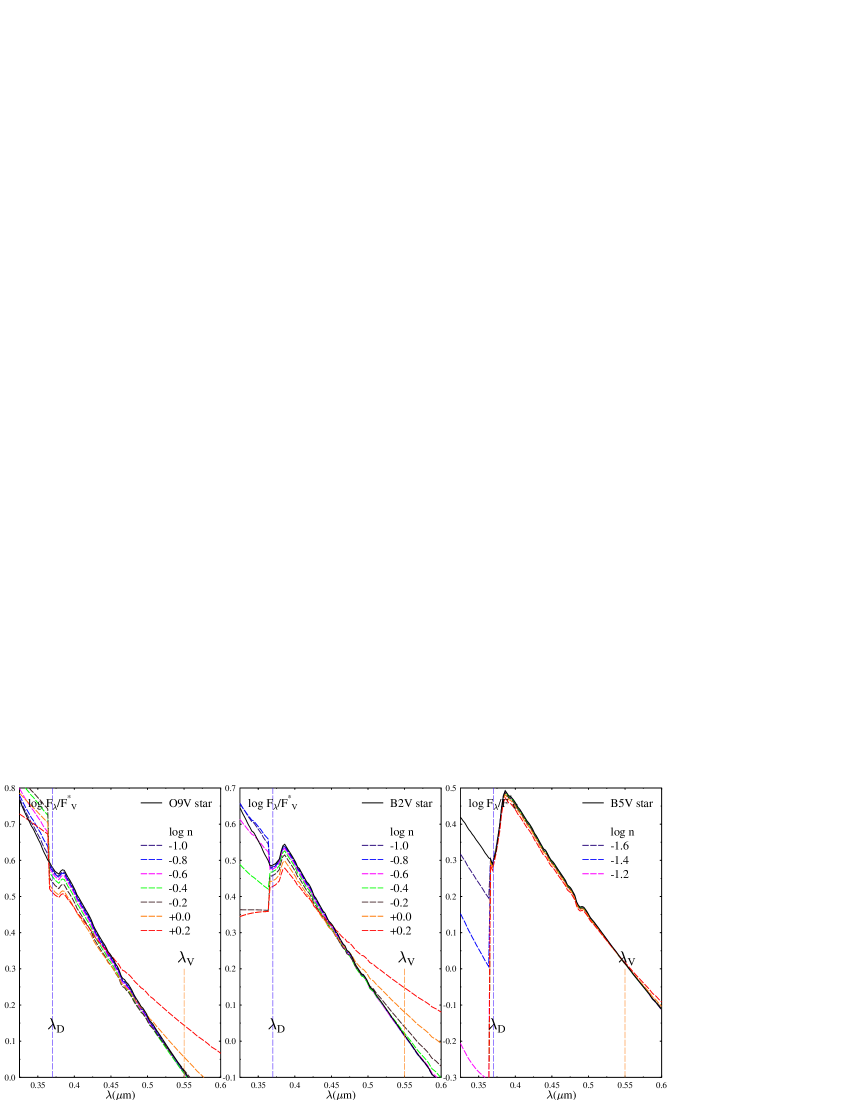
Figure 11: Changes of the energy distribution in the spectral interval $0.325\leq\lambda\leq 0.6$ $\mu$m induced by a circumstellar disc around stars of spectral type O9V, B2V and B5V. In the figure are indicated the wavelength $\lambda_{D}$ at which is measured $D_{*}$, and the central wavelength $\lambda_{V}$ of the $V$ magnitude. In the column $\log n$, $n$ is given in units of $N/10^{12}$ with $[N]=$ cm^-3

To simplify the calculations, we have adopted the average radial temperature distribution in the circumstellar disc derived in Moujtahid et al. (2000a), while its density follows the power-law deduced in Zorec et al. (2007) that was needed to account for the F ii emission lines. For the models shown in Fig. 11 we used stellar spectra given by Kurucz (1993) for: $T_{\rm eff}=30\,000$ K, $\log g=4.0$ (O9V); $T_{\rm eff}=22\,500$ K, $\log g=4.0$ (B2V); and $T_{\rm eff}=15\,000$ K, $\log g=4.0$ (B5V). In these models, the spectral region near $F^{+}_{\lambda_{D}}$ is only sketched to avoid detailed calculations of the level occupation probabilities in the upper hydrogen atomic level and the corresponding truncation of partition functions (Hummer & Mihalas 1988) that would necessarily allow for the still badly-mastered non-ideal effects (Rohrmann & Zorec 2006).

Table 7: Measurement errors induced by the circumstellar emission/absorption on the estimate of the photospheric component $D_{*}$ BD and on the corresponding absolute magnitude $M_{\rm V}(\lambda_{1},D_{*})$ determination.

$\log N/10^{12}$		$-1.0$	$-0.8$	$-0.6$	$-0.4$	$-0.2$	$0.0$	$+0.2$
Sp.T	$D_{*}$	$D^{\rm obs}_{*}-D_{*}$
O8V	0.049	0.000	0.000	$-0.001$	$-0.002$	$-0.005$	$-0.012$	$-0.023$
B2V	0.130	0.000	$-0.001$	$-0.002$	$-0.004$	$-0.009$	$-0.020$	$-0.038$
$\log N/10^{12}$		$-1.6$	$-1.4$	$-1.2$	$-1.0$	$-0.8$	$-0.6$	$-0.4$
B5V	0.261	0.000	0.000	0.000	0.000	$-0.001$	$-0.002$	$-0.005$
		$\delta M_{\rm V}$
O8V		$-0.01$	$-0.02$	$-0.02$	$-0.04$	$-0.09$	$-0.21$	$-0.41$
O8III		$-0.01$	$-0.01$	$-0.00$	$-0.03$	$-0.07$	$-0.16$	$-0.30$
B2V		$-0.01$	$-0.02$	$-0.02$	$-0.06$	$-0.14$	$-0.30$	$-0.60$
B2III		$-0.01$	$-0.02$	$-0.02$	$-0.04$	$-0.10$	$-0.23$	$-0.45$
B5V		0.00	0.00	0.00	0.00	$-0.01$	$-0.02$	$-0.06$
B5III		0.00	0.00	0.00	0.00	$-0.01$	$-0.02$	$-0.05$

The spectrophotometric behaviours shown in Fig. 11 are an excerpt of many others that can be obtained just by changing the aspect angle $i$. The amount of continuum emission and absorption also depends on the size and opening angle of the lemniscat-like shaped circumstellar envelope. As much as it concerns the present models, it is rather difficult to obtain shell-phase in very hot stars. On the contrary, Be and shell phases can be obtained easily for B2-type objects, and late type B would rather display shell aspects. According to the effective temperature among early type CBe stars, the emission in the second BD is accompanied either by a reddening or a blueing of the Paschen continuum. In late type CBe stars, the shell-absorption seems not to be accompanied by any significant change of in colour of the Paschen continuum energy distribution. In all these cases, we can note that when the emission or the absorption in the second BD vary a lot, the phospheric energy jump at the BD remains remarkably unchanged.

In Table 7 we present the values of $D_{*}$ for the unperturbed stars, as well as the errors $\delta D_{*}=D_{*}^{\rm obs}-D_{*}$ committed on the $D_{*}$-determination carried by the effects a) and b) described above. Because we are not interested in giving detailed physical interpretations of the calculated effects, the parameter $\log n$ must be regarded only as a way to produce a given amount of continuum emission or absorption. We should thus pay attention only on these amounts and conclude that the events labeled with $\log n=0.0$ and $+0.2$ are rather extreme and rarely observed. In this respect, we note that in the compilation made by Moujtahid et al. (1998), which actually corresponds to spotted measurements concerning otherwise long-term Be-star ”bumper” activity (Cook et al. 1995; Hubert & Floquet 1998; Hubert et al. 2000; Keller et al. 2002; Mennickent et al. 2002; de Wit et al. 2006), the magnitude changes are of the order of $0.1\lesssim\Delta V\lesssim 0.2$ mag and rarely as high as $\Delta V\lesssim 0.5$ mag.

In the lower part of Table 7 we also give the errors $\delta M_{\rm V}$ that $\delta D_{*}$ values would produce on the visual absolute magnitude $M_{\rm V}(\lambda_{1},D_{*})$. We notice that in all cases the $\delta M_{\rm V}$ errors are smaller than the amplitude of $M_{\rm V}(\lambda_{1},D_{*})$ values that may concern a single average MK spectral type (Zorec & Briot 1991).

Let us finally mention that errors made on the estimate of $D_{*}$ can be somewhat reduced if the colour effect acting on the extrapolated $F^{+}_{\lambda_{D}}$ flux, which resembles that of an increased interstellar extinction, is taken into account by using

$$\begin{array}[]{rcl}\displaystyle D_{*}&=&D_{*}^{\rm obs}+\Delta D_{*}\\ \displaystyle\Delta D_{*}&=&a\times[\Phi^{\rm obs}-\Phi(\lambda_{1},D^{o}_{*})],\end{array}$$ (8)

where $a=0.02$, if the Paschen colour gradient is $\Phi=\Phi_{\rm rb}$ of the BCD system. This relation was derived by the creators of the BCD system (Divan 1954), and since then applied to every determination of the BD when the ISM extinction detected by a high gradient difference $\Delta\Phi=\Phi^{\rm obs}-\Phi(\lambda_{1},D_{*})]$. In extreme cases $\Delta\Phi\simeq 0.5$ $\mu$m, the use of Eq. (8) can reduce the largest uncertainties $\delta D_{*}$ given in Table 7 to the the standard BCD uncertainty $\delta D\lesssim 0.015$ dex.

It is finally worth noting that the change of $\lambda_{1}$ due to $\delta D_{*}$ and the variation of the slope of the Paschen continuum is extremely small and thus negligible.

Appendix B Evaluation of the flux calibration of the FLWO/FAST spectra

The determination of reliable physical parameters of stars by means of the BCD system methods requires the spectra to have at least an accurate relative flux calibration. In this appendix we present an evaluation of the flux calibration of the FLWO/FAST sample, by comparing different spectra of the same objects. In the discussion below we analyse only the spectral region between 3 700 and 4 600 $\AA$, where the BCD parameters are measured. For some spectra drops in the signal-to-noise and large differences in the flux calibrations at shorter wavelengths are apparent. However, as explained in Sects. 2.1 and 3.1, they don’t have any impact in the determination of the physical parameters of the stars.

For 31 stars we have two spectra obtained at different epochs, and for one more, star 181, we have three spectra. All these spectra are presented in Figs. 12 to 15. For each object we present two panels. In the upper one we overplot the two- or three- flux calibrated and normalised spectra in a logarithmic scale. In the bottom panel we represent the difference between the normalised fluxes as a function of the wavelength.

From the comparison between the spectra we can divide the object sample into three groups. Group A is composed of the stars for which the two calibrated spectra overlap, indicating that the flux calibrations applied to each spectrum are consistent. It includes 14 objects, namely stars 23, 56, 68, 110, 118, 124, 161, 170, 171, 179, 181, 210, 219 and 223. Group B is composed of the stars displaying differences between the spectra, which imply differences between the flux calibrations, but the difference is a lineal function of the wavelength, as shown in the bottom panel for each star. Group B includes 16 objects, namely stars 109, 116, 127, 130, 153, 154, 164, 169, 172, 183, 185, 188, 211, 214, 217, and 218. Finally, Group C is composed by two more objects, stars 204 and 207, which show differences in the flux calibration which are not a lineal function of the wavelength.

The differences in the flux calibration present in the stars of Group B do not have any effect on the determination of the $D$ and $\lambda_{1}$ parameters. If the difference between the two spectra increases linearly with the decreasing wavelength, the variation of the Paschen continuum extrapolated at 3 700 $\AA$ exactly compensates the variation of the bottom of the Balmer discontinuity at the same wavelength, and the position of the discontinuity is not affected. The mean differences between the $D$ and $\lambda_{1}$ parameters for stars of Group A are $28\pm 24$ dex and $7.0\pm 6.0$ $\AA$ respectively, while for stars of Group B these are $31\pm 22$ dex and $7.4\pm 5.4$ $\AA$ respectively.

These differences do, however, affect the determination of the interstellar reddening. The reddening value is derived from the $\Phi_{b}$ parameter, which measures the slope of the Paschen continuum. This slope is sensitive to differences in the relative flux calibration. The mean difference in the determination of $E(B-V)$ for stars in the Group A is $0.06\pm 0.04$ mag., while for stars in Group B it amounts to $0.15\pm 0.10$ mag. This last figure is consistent with the standard deviation obtained when comparing our $E(B-V)$ values with values in the literature for the same stars presented in Sect. 4, and can be considered as the mean error of our $E(B-V)$ determination.

For stars in Group C the flux calibrations are not consistent. This represents up to four spectra out of 65 analysed in this appendix. In addition, it should be noted that the differences between the calibrations are small, and translate into mean differences of the parameters determined from them well within 3$\sigma$ of the mean errors considered in this paper.

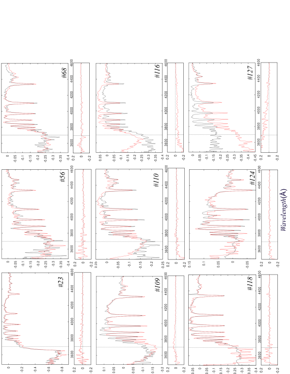
Figure 12: Stars with two or more spectra. For each object the upper panel represents the overplot of the spectra and the lower panel the difference between the two spectra.

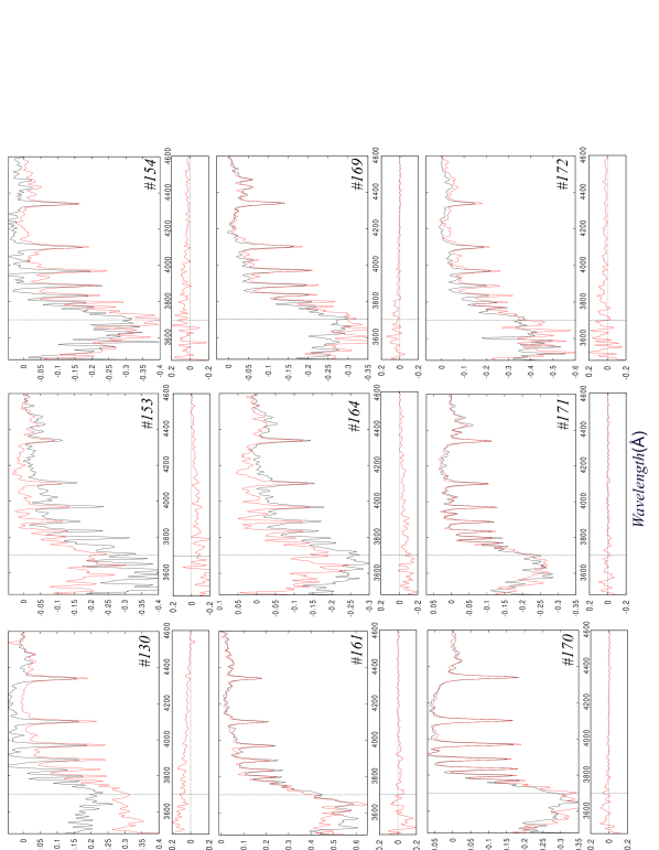
Figure 13: As Fig. 12.

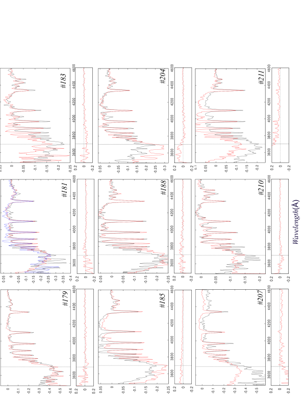
Figure 14: As Fig. 12.

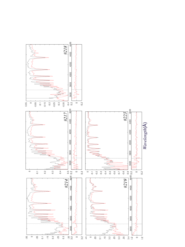
Figure 15: As Fig. 12.

References

- Aidelman et al. (2012) Aidelman, Y., Cidale, L. S., Zorec, J., & Arias, M. L. 2012, A&A, 544, A64
- Allen (1973) Allen, C. W. 1973, Astrophysical quantities
- Balona & Shobbrook (1984) Balona, L. A. & Shobbrook, R. R. 1984, MNRAS, 211, 375
- Barbier (1948) Barbier, D. 1948, Annales d’Astrophysique, 11, 13
- Barbier & Chalonge (1939) Barbier, D. & Chalonge, D. 1939, ApJ, 90, 627
- Barbier & Chalonge (1941) Barbier, D. & Chalonge, D. 1941, Annales d’Astrophysique, 4, 30
- Barentsen et al. (2014) Barentsen, G., Farnhill, H. J., Drew, J. E., et al. 2014, MNRAS, 444, 3230
- Carciofi et al. (2009) Carciofi, A. C., Okazaki, A. T., Le Bouquin, J.-B., et al. 2009, A&A, 504, 915
- Chalonge & Divan (1952) Chalonge, D. & Divan, L. 1952, Annales d’Astrophysique, 15, 201
- Chalonge & Divan (1973) Chalonge, D. & Divan, L. 1973, A&A, 23, 69
- Cochetti (2014) Cochetti, Y. R. 2014, Tésis de Licenciatura, Estudio observacional de la segunda discontinuidad de Balmer en estrellas Be y Bn (Universidad Nacional de La Plata)
- Cook et al. (1995) Cook, K. H., Alcock, C., Allsman, H. A., et al. 1995, in Astronomical Society of the Pacific Conference Series, Vol. 83, IAU Colloq. 155: Astrophysical Applications of Stellar Pulsation, ed. R. S. Stobie & P. A. Whitelock, 221
- Crawford (1978) Crawford, D. L. 1978, AJ, 83, 48
- Dachs et al. (1988) Dachs, J., Kiehling, R., & Engels, D. 1988, A&A, 194, 167
- De Loore et al. (1979) De Loore, C., Hensberge, H., Sterken, C., et al. 1979, A&A, 78, 287
- de Wit et al. (2006) de Wit, W. J., Lamers, H. J. G. L. M., Marquette, J. B., & Beaulieu, J. P. 2006, A&A, 456, 1027
- Divan (1954) Divan, L. 1954, Annales d’Astrophysique, 17, 456
- Divan & Zorec (1982a) Divan, L. & Zorec, J. 1982a, in IAU Symposium, Vol. 98, Be Stars, ed. M. Jaschek & H.-G. Groth, 61–63
- Divan & Zorec (1982b) Divan, L. & Zorec, J. 1982b, in ESA Special Publication, Vol. 176, Third European IUE Conference, ed. E. Rolfe & A. Heck, 291–293
- Divan et al. (1983) Divan, L., Zorec, J., & Andrillat, Y. 1983, A&A, 126, L8
- Drew et al. (2005) Drew, J. E., Greimel, R., Irwin, M. J., et al. 2005, MNRAS, 362, 753
- Fabregat & Capilla (2005) Fabregat, J. & Capilla, G. 2005, MNRAS, 358, 66
- Fabregat & Torrejón (1998) Fabregat, J. & Torrejón, J. M. 1998, A&A, 332, 643
- Fabricant et al. (1998) Fabricant, D., Cheimets, P., Caldwell, N., & Geary, J. 1998, PASP, 110, 79
- Fiorucci & Munari (2003) Fiorucci, M. & Munari, U. 2003, A&A, 401, 781
- Gray & Corbally (2009) Gray, R. O. & Corbally, J., C. 2009, Stellar Spectral Classification
- Hubert & Floquet (1998) Hubert, A. M. & Floquet, M. 1998, A&A, 335, 565
- Hubert et al. (2000) Hubert, A. M., Floquet, M., & Zorec, J. 2000, in Astronomical Society of the Pacific Conference Series, Vol. 214, IAU Colloq. 175: The Be Phenomenon in Early-Type Stars, ed. M. A. Smith, H. F. Henrichs, & J. Fabregat, 348
- Hummer & Mihalas (1988) Hummer, D. G. & Mihalas, D. 1988, ApJ, 331, 794
- Kaiser (1989) Kaiser, D. 1989, A&A, 222, 187
- Keller et al. (2002) Keller, S. C., Bessell, M. S., Cook, K. H., Geha, M., & Syphers, D. 2002, AJ, 124, 2039
- Kurucz (1993) Kurucz, R. 1993, ATLAS9 Stellar Atmosphere Programs and 2 km/s grid. Kurucz CD-ROM No. 13. Cambridge, Mass.: Smithsonian Astrophysical Observatory, 1993., 13
- Mennickent et al. (2002) Mennickent, R. E., Pietrzyński, G., Gieren, W., & Szewczyk, O. 2002, A&A, 393, 887
- Monguió et al. (2013) Monguió, M., Figueras, F., & Grosbøl, P. 2013, A&A, 549, A78
- Moon (1986) Moon, T. 1986, Ap&SS, 122, 173