Some results
on the computing of Tukey’s halfspace medain

Summary

Depth of the Tukey median is investigated for empirical distributions. A sharper upper bound is provided for this value for data sets in general position. This bound is lower than the existing one in the literature, and more importantly derived under the fixed sample size practical scenario. Several results obtained in this paper are interesting theoretically and useful as well to reduce the computational burden of the Tukey median practically when $p$ is large relative to large $n$.

Key words: Data depth; Tukey median; maximum halfspace depth; general position

2000 Mathematics Subject Classification Codes: 62F10; 62F40; 62F35

1 Introduction

For a univariate random sample $\mathcal{Z}^{n}=\{Z_{1},Z_{2},\cdots,Z_{n}\}$, let $Z_{(1)},Z_{(2)},\cdots,Z_{(n)}$ be the corresponding ordered statistics such that $Z_{(1)}\leq Z_{(2)}\leq\cdots\leq Z_{(n)}$. The sample median is then defined as

$$\mu(\mathcal{Z}^{n})=\frac{Z_{(\lfloor(n+1)/2\rfloor)}+Z_{(\lfloor(n+2)/2\rfloor)}}{2},$$

where $\lfloor\cdot\rfloor$ denotes the floor function. In the literature, $\mu(\mathcal{Z}^{n})$ is well known for its robustness. In fact, it has the highest possible breakdown point among its competitors and a bounded influence function. Hence, it usually serves as an alterative to the sample mean for data sets containing outliers (or with heavy tails).

To extend the concept to multivariate setting is desirable. The univariate definition depends on the ordered statistics, whereas no natural ordering exists in the multivariate setting. It is thus nontrivial to extend it to multidimensional setting in $\mathcal{R}^{p}$ with $p\geq 2$. Several extensions, such as coordinatewise median (Bickel, 1964) and spatial median (Weber , 1909) and (Brown, 1983), etc., exist in the literature though. They lack the desirable affine equivariance, nevertheless. See Small (1990) for an early summary on multivariate medians.

Observing the fact that $\mu(\mathcal{Z}^{n})$ is the average of all points maximizing the function

$$t\rightarrow\min\left\{P_{n}(Z\leq t),P_{n}(Z\geq t)\right\}=\min_{u\in\{-1,1\}}P_{n}(uZ\leq ut),$$

where $Z$ is a univariate random variable and $P_{n}$ stands for the empirical distribution function, Tukey (1975) heuristically proposed a notion of depth function. He first defined the depth of a point x with respect to $\mathcal{X}^{n}$ as

$$D(\textbf{\emph{x}},\mathcal{X}^{n})=\inf_{\textbf{\emph{u}}\in\{\textbf{\emph{z}}:\|\textbf{\emph{z}}\|=1\}}P_{n}(\textbf{\emph{u}}^{\top}X\leq\textbf{\emph{u}}^{\top}\textbf{\emph{x}}),$$ (1)

where $\mathcal{X}^{n}=\{X_{1},X_{2},\cdots,X_{n}\}$ is a $p$-variate random sample, $X$ is a random variable in $R^{p}$ and $\|\cdot\|$ stands for Euclidean norm, and then proposed to consider the average of such points that maximize $D(\textbf{\emph{x}},\mathcal{X}^{n})$ with respect to x as the multivariate median (more specially, hereafter Tukey median). That is,

$$T^{*}(\mathcal{X}^{n})=\textbf{Ave}\left\{\textbf{\emph{x}}\in\mathcal{R}^{p}:D(\textbf{\emph{x}},\mathcal{X}^{n})=\lambda^{*}(\mathcal{X}^{n})\right\},$$

where $\lambda^{*}(\mathcal{X}^{n})=\sup_{\textbf{\emph{x}}}D(\textbf{\emph{x}},\mathcal{X}^{n})$. See also Donoho and Gasko (1992) (hereafter DG92) for details. But slightly differently, DG92’s discussions are based on an integer valued function, i.e., $nD(\textbf{\emph{x}},\mathcal{X}^{n})$, instead.

$T^{*}(\mathcal{X}^{n})$ inherits many advantages of the univariate median. For example, it has an asymptotical breakdown point as high as $1/3$ under the centro-symmetric assumption. Unlike the aforementioned generalizations, $T^{*}(\mathcal{X}^{n})$ is affine equivariant. That is,

$$T^{*}(\mathbb{A}\mathcal{X}^{n}+\textbf{\emph{b}})=\mathbb{A}T^{*}(\mathcal{X}^{n})+\textbf{\emph{b}}$$

for all full-rank $p\times p$ matrices $\mathbb{A}$ and $p$-vectors b. Here $\mathbb{A}\mathcal{X}^{n}=\{\mathbb{A}X_{1},\mathbb{A}X_{2},\cdots,\mathbb{A}X_{n}\}$. Since data transformations, such as rotation and rescaling, are very common in practice, this property is very important and often expected for a multivariate location estimator.

Unfortunately, $T^{*}(\mathcal{X}^{n})$ is computationally intensive. Approximate algorithm has been developed by Struyf and Rousseeuw (2000) though. This algorithm is lack of affine equivariance, nevertheless. While, on the other hand, efficient exact algorithm exists, but is only feasible for bivariate data (Rousseeuw and Ruts, 1998; Miller et al., 2003).

Following DG92, define the $\alpha$th depth contour/region as $D_{\tau}:=\{\textbf{\emph{x}}\in\mathcal{R}^{p}:D(\textbf{\emph{x}},\mathcal{X}^{n})\geq\tau\}$. To avoid unbounded as well as empty regions, hereafter $D_{\tau}$ is restricted to $0<\tau\leq\lambda^{*}(\mathcal{X}^{n})$ (Lange et al., 2014). Note that $T^{*}(\mathcal{X}^{n})$ is in fact the average of all points in the most central (deepest) region, hereafter median region,

$$\mathcal{M}(\mathcal{X}^{n})=\left\{\textbf{\emph{x}}\in\mathcal{R}^{p}:D(\textbf{\emph{x}},\mathcal{X}^{n})=\lambda^{*}(\mathcal{X}^{n})\right\}.$$

Computing $T^{*}(\mathcal{X}^{n})$ is in fact a special case of computing the depth regions. For a fixed depth value $\tau$, there have been some exact algorithms developed for computing the depth region (Paindaveine and Šiman, 2012a, b; Ruts and Rousseeuw, 1996). However, the maximum Tukey depth $\lambda^{*}(\mathcal{X}^{n})$ is usually unknown in advance. Hence, how to determine $\lambda^{*}(\mathcal{X}^{n})$ is the most key issue for exactly computing $T^{*}(\mathcal{X}^{n})$.

To obtain this value, based on DG92’s lower and upper bounds results, conventionally one needs to search over the interval $[\lceil n/(p+1)\rceil/n,\lceil n/2\rceil/n]$ step by step as suggested and did in Rousseeuw and Ruts (1998), where $\lceil\cdot\rceil$ denotes the ceiling function. During this process, a lot of depth regions has to be computed. Usually, computing a single depth region is very time-consuming especially when $p$ is large. Therefore, the computation would be greatly benefited in the practice by narrowing the search scope of the maximum Tukey depth, if possible.

DG92 pointed out that the lower bound $\lceil n/(p+1)\rceil/n$ of $D(x,\mathcal{X}^{n})$ is attained for some special data sets in general position, and hence can not be further improved. Is there any room of improvement for the upper bound $\lceil n/2\rceil/n$ given in DG92?

The upper bound $\lceil n/2\rceil/n$ does not depend on the dimension $p$. Intuitively, this is not sensible for computing Tukey median when $p$ is increasing. Because for a data set with fixed $n$, an increasing proportion of observations will be pushed onto the boundary of the convex hull of the data points when $p$ increases (Hastie et al., 2008). Hence, the maximum depth value may decrease. The upper bound given by DG fails to reflect this change in trend.

In this paper, we provide a sharper upper bound ${\lfloor(n-p+2)/2\rfloor}/{n}$ which may be much less than $\lceil n/2\rceil/n$ when $p$ is large relative to large $n$. For example, when $n=5p$ with $p=5$, the search range of the maximum Tukey depth can be reduced by more than one quarter. As for the choice of $n=5p$, a justification is given on p.326 of Juan and Prieto (1995); see also Zuo (2004).

Since the computation of the depth of a single point is of less time complexity than that of computing a Tukey depth contour (Liu and Zuo, 2014; Dyckerhoff and Mozharovskyi, 2016), and the depth of sample points is easily obtained as by-product of computing the depth contour, one may wonder if the deepest observation could serve as a Tukey median. This paper also considers this problem and provides a definite answer.

We show that the sample observation can not lie in the interior of the median region. It can be included in the median region only if it is a vertex of the convex set. Hence, unless median region is a singleton, a sample point can not serve as the Tukey median in general.

To guarantee the uniqueness of Tukey’s median for the population distributions, some symmetry assumption is commonly imposed( see, e.g., DG92, and Zuo and Serfling (2000a)(ZS00a)). The weakest version of symmetry is so-called ‘halfspace symmetry’(see ZS00a). Another common assumption on underlying data when one deals with breakdown point robustness or data depth is ‘in general position’ (see DG92). An interesting byproduct of the paper is the conclusion: that ‘in general position’ and ‘halfspace symmetry’ could not coexist for a data set in three or higher dimensions, even if there is a central symmetric underlying distribution, e.g., normal distribution.

The rest paper is organized as follows. Section 2 establishes a sharper upper bound for the halfspace depth of Tukey median. Section 3 is devoted to provide a definite answer to the question: Can a sample point serve as Tukey median? Concluding remarks end the paper.

2 The upper bound for the Tukey depth

In this section, we investigate the maximum Tukey depth. In the sequel we will always assume that data set is in general position. A $p$-variate data set is called to be in general position if there are no more than $p$ sample points in any $(p-1)$-dimensional hyperplane. This assumption is often adopted in the literature when dealing with the data depth and breakdown point; see, e.g., Donoho and Gasko (1992); Mosler et al. (2009), among others.

Observe that $n$ and the data cloud $\mathcal{X}^{n}$ are fixed in the following. For convenience, we drop the argument $\mathcal{X}^{n}$ from $T^{*}(\mathcal{X}^{n})$, $\lambda^{*}(\mathcal{X}^{n})$, $\mathcal{M}(\mathcal{X}^{n})$ and $D(x,\mathcal{X}^{n})$ if no confusion arises. Besides, we introduce a few other notations as follows. Let $\kappa^{*}=n\lambda^{*}$. Obviously, $\kappa^{*}$ is a positive integer since the image of $P_{n}$ only can take a finite set of values $\{0,1/n,2/n,\cdots,1\}$. For any $k$ points $\{\mathbf{x}_{1},\mathbf{x}_{2},\cdots,\mathbf{x}_{k}\}$, picking an arbitrary point, without loss of generality, say, $\mathbf{x}_{k}$, we denote $\textbf{span}(\mathbf{x}_{l}|l=1,2,\cdots,k)=\{\sum_{l=1}^{p-1}\lambda_{l}(\mathbf{x}_{l}-\mathbf{x}_{k}):\forall\lambda_{i}\in\mathcal{R}^{1}\}$ as the subspace spanned by $\mathbf{x}_{1}-\mathbf{x}_{k},\mathbf{x}_{2}-\mathbf{x}_{k},\cdots,\mathbf{x}_{k-1}-\mathbf{x}_{k}$. (For $k=1$, we assume $\textbf{span}(\mathbf{x}_{l})=\{\mathbf{0}\}$.)

The following representation of $\mathcal{M}$ will be repeatedly utilized in the sequel. Following Theorem 4.2 in Paindaveine and Šiman (2011), a finite number of direction vectors suffice for determining the sample Tukey regions, which include the median region as a special case. That is, let $\{\textbf{\emph{u}}_{1}^{*},\textbf{\emph{u}}_{2}^{*},\cdots,\textbf{\emph{u}}_{m}^{*}\}$ be all normal vectors of the hyperplanes, with each of which passing through $p$ observations and cutting off exactly $\kappa^{*}-1$ observations, then we have

$$\mathcal{M} = \bigcap_{j=1}^{m}\left\{\textbf{\emph{x}}:(\textbf{\emph{u}}_{j}^{*})^{\top}\textbf{\emph{x}}\geq q_{j}\right\},\quad\text{where}$$ (2)

$$q_{j} = \inf\left\{t\in\mathcal{R}^{1}:P_{n}((\textbf{\emph{u}}_{j}^{*})^{\top}X\leq t)\geq\lambda^{*}\right\}.$$

The following theorem provides a sharp upper bound for the maximum Tukey depth.

Theorem 1. Suppose $\mathcal{X}^{n}\subset\mathcal{R}^{p}$ ($n>p$) is in general position. We have

$$\lambda^{*}\leq\left\{\begin{array}[]{lcl}\frac{\lfloor(n-p+2)/2\rfloor}{n},&&\textbf{dim}(\mathcal{M})<p,\\ &&\\ \frac{\lfloor(n-p+1)/2\rfloor}{n},&&\textbf{dim}(\mathcal{M})=p,\\ \end{array}\right.$$

where $\textbf{dim}(\mathcal{M})$ denotes the affine dimension of $\mathcal{M}$.

Since the proof is trivial for $p=1$, we focus only on $p\geq 2$ in the sequel. For convenience, we present the long proof in two parts, i.e., (I) and (II). The basic idea is that: In Part (I), if $\mathcal{M}$ is of affine dimension $p$, i.e., has nonzero volume, one can always deviate (shift) the separating hyperplane around some points in $\mathcal{M}$ to get rid of $p-1$ sample points in it; See 1(a). In Part (II), as $\mathcal{M}$ is of affine dimension less than $p$, i.e., has volume zero, $T^{*}$ lies in a hyperplane through $p$ observations (not more because of the general position assumption), and thus one can not always cut off all of these $p$ observations because one point should remain in the lower mass halfspace; See 1(b).

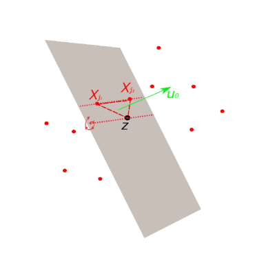
(a) Illustration for Part (I)

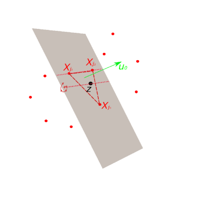
(b) Illustration for Part (II)

Figure 1: Shown are illustrations for the main idea of the proofs of Part (I) (left) and (II) (right) of Theorem 1, where the small points denote the observations, the big point denote z, and $\textbf{\emph{u}}_{0}$ the vector normal to the separating hyperplane, which passes through tow observations in the left case, but three observations in the right case.

Proof of Theorem 1. (I) $\textbf{dim}(\mathcal{M})=p$: Observe that $\mathcal{X}^{n}$ is a finite sample in general position, and $\mathcal{M}$ is a convex polytope of affine dimension $p$. Hence, it is easy to check that there exists a point $\textbf{\emph{z}}_{1}\in\mathcal{M}$ such that $\{\textbf{\emph{z}}_{1}\}\cup\mathcal{X}^{n}$ is in general position.

Using this, we claim that the hyperplane $\Pi_{1}$ passing through $\{\textbf{\emph{z}}_{1},X_{j_{1}},X_{j_{2}},\cdots,X_{j_{p-1}}\}$ contains only $p-1$ observations of $\mathcal{X}^{n}$ for an any given set of $\{X_{j_{1}},X_{j_{2}},\cdots,X_{j_{p-1}}\}$. Let $\textbf{\emph{u}}_{1}$ be $\Pi_{1}$’s normal vector such that $P_{n}(u_{1}^{\top}X<\textbf{\emph{u}}_{1}^{\top}z_{1})=\min\{P_{n}(\textbf{\emph{u}}_{1}^{\top}X<\textbf{\emph{u}}_{1}^{\top}\textbf{\emph{z}}_{1}),P_{n}(-\textbf{\emph{u}}_{1}^{\top}X<-\textbf{\emph{u}}_{1}^{\top}z_{1})\}$. Obviously, $\textbf{\emph{u}}_{1}^{\top}\textbf{\emph{z}}_{1}=\textbf{\emph{u}}_{1}^{\top}X_{j_{1}}=\cdots=\textbf{\emph{u}}_{1}^{\top}X_{j_{p-1}}$ and $P_{n}(\textbf{\emph{u}}_{1}^{\top}X<\textbf{\emph{u}}_{1}^{\top}\textbf{\emph{z}}_{1})\leq\left\lfloor\frac{n-(p-1)}{2}\right\rfloor\big{/}n$.

Let $\mathbf{V}=\textbf{span}(X_{j_{k}}|k=1,2,\cdots,p-1)$. Now, we proceed to show that, if $\textbf{\emph{z}}_{1}\notin\mathbf{V}$, it is possible to get rid of $X_{j_{1}},X_{j_{2}},\cdots,X_{j_{p-1}}$ from $\Pi_{1}$ through deviating it around $\textbf{\emph{z}}_{1}$.

Decompose $\textbf{\emph{v}}_{1}:=\textbf{\emph{z}}_{1}-X_{j_{1}}=\textbf{\emph{v}}_{1}^{\prime}+\textbf{\emph{v}}_{1}^{\prime\prime}$, where $\textbf{\emph{v}}_{1}^{\prime}\in\mathbf{V}$ and $\textbf{\emph{v}}_{1}^{\prime\prime}\in\mathbf{V}^{\bot}$. Here $\mathbf{V}^{\bot}$ denotes the orthogonal complement space of $\mathbf{V}$. Obviously, $\textbf{\emph{v}}_{1}^{\prime\prime}\neq 0$. (If not, $\textbf{\emph{v}}_{1}^{\prime}=\textbf{\emph{z}}_{1}-X_{j_{1}}\in\mathbf{V}$, contradicting with that $\{\textbf{\emph{z}}_{1}\}\cup\mathcal{X}^{n}$ is in general position.) Similarly to Dyckerhoff and Mozharovskyi (2016), let

$$\varepsilon=\frac{1}{2}\min_{l\in\{1,\,2,\,\cdots,\,n\}\setminus\{j_{1},\,j_{2},\,\cdots,\,j_{p-1}\}}\frac{|\textbf{\emph{u}}_{1}^{\top}(\textbf{\emph{z}}_{1}-X_{l})|}{|(\textbf{\emph{v}}_{1}^{\prime\prime})^{\top}(\textbf{\emph{z}}_{1}-X_{l})|},$$ (4)

and $\widetilde{\textbf{\emph{u}}}_{1}=\textbf{\emph{u}}_{1}-\varepsilon\textbf{\emph{v}}_{1}^{\prime\prime}$. Here we define $|\textbf{\emph{u}}_{1}^{\top}(\textbf{\emph{z}}_{1}-X_{i})|/|(\textbf{\emph{v}}_{1}^{\prime\prime})^{\top}(\textbf{\emph{z}}_{1}-X_{i})|=+\infty$ if $(\textbf{\emph{v}}_{1}^{\prime\prime})^{\top}(\textbf{\emph{z}}_{1}-X_{i})=0$. Then $|\varepsilon(\textbf{\emph{v}}_{1}^{\prime\prime})^{\top}(\textbf{\emph{z}}_{1}-X_{i})|<|\textbf{\emph{u}}_{1}^{\top}(\textbf{\emph{z}}_{1}-X_{i})|$, and in turn

$$\text{sgn}(\widetilde{\textbf{\emph{u}}}_{1}^{\top}(\textbf{\emph{z}}_{1}-X_{i}))=\text{sgn}(\textbf{\emph{u}}_{1}^{\top}(\textbf{\emph{z}}_{1}-X_{i})),\quad i\in\{1,\,2,\,\cdots,\,n\}\setminus\{j_{1},\,j_{2},\,\cdots,\,j_{p-1}\},$$ (5)

where sgn$(\cdot)$ denotes the sign function. On the other hand, (a) $\widetilde{\textbf{\emph{u}}}_{1}^{\top}(\textbf{\emph{z}}_{1}-X_{j_{1}})=-\varepsilon\|\textbf{\emph{v}}_{1}^{\prime\prime}\|^{2}<0$, and (b) for each $k=2,3\cdots,p-1$, $\widetilde{\textbf{\emph{u}}}_{1}^{\top}(\textbf{\emph{z}}_{1}-X_{j_{k}})=\widetilde{\textbf{\emph{u}}}_{1}^{\top}(\textbf{\emph{z}}_{1}-X_{j_{1}}+(X_{j_{1}}-X_{j_{k}}))=-\varepsilon\|\textbf{\emph{v}}_{1}^{\prime\prime}\|^{2}<0$. Then $\widetilde{\textbf{\emph{u}}}_{1}^{\top}\textbf{\emph{z}}_{1}<\widetilde{\textbf{\emph{u}}}_{1}^{\top}X_{j_{1}},\widetilde{\textbf{\emph{u}}}_{1}^{\top}X_{j_{2}},\cdots,\widetilde{\textbf{\emph{u}}}_{1}^{\top}X_{j_{p-1}}$. These, together with (5), lead to $P_{n}(\widetilde{\textbf{\emph{u}}}_{1}^{\top}X\leq\widetilde{\textbf{\emph{u}}}_{1}^{\top}\textbf{\emph{z}}_{1})=P_{n}(\textbf{\emph{u}}_{1}^{\top}X<\textbf{\emph{u}}_{1}^{\top}\textbf{\emph{z}}_{1})$. Hence,

$$\lambda^{*}=D(\textbf{\emph{z}}_{1})\leq P_{n}(\widetilde{\textbf{\emph{u}}}_{1}^{\top}X\leq\widetilde{\textbf{\emph{u}}}_{1}^{\top}\textbf{\emph{z}}_{1})\leq\left\lfloor\frac{n-(p-1)}{2}\right\rfloor\Big{/}n.$$

(II) $\textbf{dim}(\mathcal{M})<p$: Relying on (2), we claim that there $\exists k\in\{1,2,\cdots,m\}$ such that $(\textbf{\emph{u}}_{k}^{*})^{\top}T^{*}(\mathcal{X}^{n})=q_{k}$. Using this, a simple derivation leads to $\mathcal{M}\subset\Pi_{2}:=\{z\in\mathcal{R}^{p}:(\textbf{\emph{u}}_{k}^{*})^{\top}\textbf{\emph{z}}=q_{k}\}$. Obviously, $\Pi_{2}$ should pass through $p$ observations, say $\{X_{k_{1}},X_{k_{2}},\cdots,X_{k_{p}}\}$, by the definition of $\textbf{\emph{u}}_{2}:=\textbf{\emph{u}}_{k}^{*}$ and $q_{k}$, and $P_{n}(\textbf{\emph{u}}_{2}^{\top}X<\textbf{\emph{u}}_{2}^{\top}\textbf{\emph{z}}_{2})\leq\lfloor\frac{n-p}{2}\rfloor\big{/}n$ for any $\textbf{\emph{z}}_{2}\in\mathcal{M}$.

Without confusion, assume $X_{k_{p}}=0$ by the affine equivariance of the Tukey depth. Let $\mathbf{W}_{i}=\textbf{span}(X_{k_{l}}|l\in\{1,2,\cdots,p\}\setminus\{i\})$ for $i=1,2,\cdots,p$. We now show that $\textbf{\emph{z}}_{2}$ does not lie simultaneously in all affine subspaces $\mathbf{W}_{i}$’s defined by facets of a $(p-1)$-dimensional simplex formed by $\{X_{k_{1}},X_{k_{2}},\cdots,X_{k_{p}}\}$.

For $p=2$: The proof is trivial because $\textbf{\emph{z}}_{2}-X_{k_{1}}$, $\textbf{\emph{z}}_{2}-X_{k_{2}}$ could not be $0$ simultaneously.

For $p>2$: By observing that if $\textbf{\emph{z}}_{2}=0(=X_{k_{p}})$, $\textbf{\emph{z}}_{2}\notin\mathbf{W}_{p}$ because $\mathcal{X}^{n}$ is in general position, we only focus on the case $\textbf{\emph{z}}_{2}\neq 0$ in what follows.

Suppose $\textbf{\emph{z}}_{2}\in\mathbf{W}_{i}$ for all $i=1,2,\cdots,p$, then there must exist some constants such that:

$$\left\{\begin{array}[]{cclcl}\textbf{\emph{z}}_{2}&=&\quad a_{12}X_{k_{2}}+a_{13}X_{k_{3}}+\cdots+a_{1,p-1}X_{k_{p-1}}&&(z_{2}\in\mathbf{W}_{1})\\ \textbf{\emph{z}}_{2}&=&a_{21}X_{k_{1}}+\quad a_{23}X_{k_{3}}+\cdots+a_{2,p-1}X_{k_{p-1}}&&(z_{2}\in\mathbf{W}_{2})\\ &\vdots&&&\\ \textbf{\emph{z}}_{2}&=&a_{p-1,1}X_{k_{1}}+a_{p-1,2}X_{k_{2}}+\cdots+a_{p-1,p-2}X_{k_{p-2}}&&(z_{2}\in\mathbf{W}_{p-1})\\ \textbf{\emph{z}}_{2}&=&b_{1}X_{k_{1}}+b_{2}X_{k_{2}}+\cdots+b_{p-1}X_{k_{p-1}}&&(z_{2}\in\mathbf{W}_{p}).\end{array}\right.$$ (11)

Let $(w_{1},w_{2},\cdots,w_{p-1})^{\top}$ be a solution to

$$\left(\begin{array}[]{ccccc}0&a_{21}&a_{31}&\cdots&a_{p-1,1}\\ a_{12}&0&a_{32}&\cdots&a_{p-1,2}\\ a_{13}&a_{23}&0&\cdots&a_{p-1,3}\\ \vdots&\vdots&\vdots&\ddots&\vdots\\ a_{1,p-1}&a_{2,p-1}&a_{3,p-1}&\cdots&0\end{array}\right)\left(\begin{array}[]{c}w_{1}\\ w_{2}\\ w_{3}\\ \vdots\\ w_{p-1}\end{array}\right)=\left(\begin{array}[]{c}b_{1}\\ b_{2}\\ b_{3}\\ \vdots\\ b_{p-1}\end{array}\right).$$

Then it is easy to check that $\sum_{i=1}^{p-1}w_{i}\textbf{\emph{z}}_{2}-\textbf{\emph{z}}_{2}=0$. Hence, $\sum_{i=1}^{p-1}w_{i}=1$ due to $\textbf{\emph{z}}_{2}\neq 0$. On the other hand, $\textbf{\emph{z}}_{2}\neq 0$ implies $(b_{1},b_{2},\cdots,b_{p-1})\neq 0$. Without confusion, assume $b_{i_{0}}\neq 0$ for $1\leq i_{0}\leq p-1$. Then by letting ‘the $p$-th equation’ $-$ ‘$\sum_{i=1}^{p-1}w_{i}$ $\times$ the $i_{0}$-th equation’ of (11), we can obtain

$$X_{k_{p}}=0=\textbf{\emph{z}}_{2}-\sum_{i=1}^{p-1}w_{i}\textbf{\emph{z}}_{2}=\sum_{l=1}^{p-1}b_{l}X_{k_{l}}-\sum_{i=1}^{p-1}w_{i}\sum_{l\neq i_{0}}^{p-1}a_{i_{0},l}X_{k_{l}}=:\sum_{l\neq i_{0}}^{p-1}\widetilde{b}_{l}X_{k_{l}}+b_{i_{0}}X_{k_{i_{0}}}\in\mathbf{W}_{p}.$$

This clearly contradicts with the fact $X_{k_{p}}\notin\mathbf{W}_{p}$ because $\mathcal{X}^{n}$ is in general position.

Suppose $\textbf{\emph{z}}_{2}\notin\mathbf{W}_{p}$ without confusion. Then similar to Part (I), it is possible to get rid of $X_{k_{1}},X_{k_{2}},\cdots,X_{k_{p-1}}$ from the separating hyperplane $\Pi_{2}$ through rotating it around $\textbf{\emph{z}}_{2}$, and hence $\lambda^{*}=D(\textbf{\emph{z}}_{2})\leq P_{n}(\textbf{\emph{u}}_{2}^{\top}X<\textbf{\emph{u}}_{2}^{\top}\textbf{\emph{z}}_{2})+1/n\leq\left\lfloor\frac{n-p+2}{2}\right\rfloor\big{/}n$.

This completes the proof of Theorem 1. $\Box$

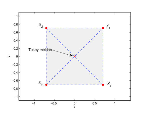
Figure 2: The maximum Tukey depth in this example is $\frac{\lfloor(4-2+2)/2\rfloor}{4}=1/2$.

Remarks
(i) The upper bound given in Theorem 1 is attained if the data set is strategically chosen; see Figure 2 for $p=2$ and Figure 6(a) for $p=3$, for example. Hence, this bound is sharp, and can not be further improved if the data are in general position. The upper bound $\lceil n/2\rceil/n$ for the maximum Tukey depth given in DG92 clearly is not sharp for $p\geq 3$ (see Figure 6(a)).

(ii) Since the upper bound is smaller than $\lceil n/2\rceil/n$ for $p\geq 3$, an interesting question is raised here about the multivariate symmetry, which is closely related to the multidimensional median.

In the literature, various notions of multivariate symmetry already exist, e.g., central symmetry, angular symmetry and halfspace symmetry. A random vector $X\in\mathcal{R}^{p}$ is said to have a distribution centrally symmetric about $\theta$ if $X-\theta$ and $\theta-X$ are equal in distribution. The angular symmetry, introduced in Liu (1990), is broader than the central symmetry. A random vector $X\in\mathcal{R}^{p}$ has a distribution angularly symmetric about $\theta$ if $(X-\theta)/\|X-\theta\|$ has a centrally symmetric distribution about the origin. Among three multivariate symmetry notions, the halfspace symmetry is the most broadening. As introduced by Zuo and Serfling (2000), a random vector $X$ has a distribution halfspace symmetric about $\theta$ if

$$P(X\in\mathcal{H}_{\theta})\geq 1/2,\text{ each closed halfspace }\mathcal{H}_{\theta}\text{ with }\theta\text{ on the boundary.}$$ (13)

It is readily to see that any one-dimensional data set is always halfspace symmetric about its median. Whether this property still holds in spaces with dimension $p>1$ is not clear without Theorem 1.

As a byproduct, Theorem 1 actually provides a negative answer to this question when $\mathcal{X}^{n}$ is in general position. By Theorem 1, for $p\geq 3$, the maximum Tukey depth is less than $1/2$ with respect to any given $\mathcal{X}^{n}$ in general position, therefore $\mathcal{X}^{n}$ could not be halfspace symmetric (and consequently not central or angular symmetric) about a point $\theta$ when $\mathcal{X}^{n}$ is in general position, even if $\mathcal{X}^{n}$ are generated from a central symmetric distribution, e.g., normal distribution. That is, the following proposition holds.

Proposition 1. In general position and halfspace symmetry could not coexist for $\mathcal{X}^{n}$ in $R^{p}$ with $p\geq 3$.

(iii) For a given data set in general position, although one does not know what is the median region nor its dimension, Theorem 1 still provides a useful guide: i.e. the maximum depth is less than $\lfloor(n-p+2)/2\rfloor/n$.

3 Can the deepest sample point serve as the Tukey median?

It is well known in the literature that computing the depth of a single point is of less time complexity than computing a Tukey depth region. Hence, it would save a lot of effort in computing and searching Tukey median if a single deepest point could serve the role. From last section, we see that $\mathcal{M}$ can be a singleton. Could a deepest sample point serve as Tukey median? Results following will answer the question.

Theorem 2. Suppose $\mathcal{X}^{n}$ is in general position. If there exists an observation $X_{l}$ ($1\leq l\leq n$) such that $D(X_{l})=\lambda^{*}$, then $X_{l}$ must be a vertex of $\mathcal{M}$.

Proof. Denote $d:=\textbf{dim}(\mathcal{M})$. Clearly, $0\leq d\leq p$. When $d=0$, the proof is trivial because $\mathcal{M}$ is a singleton. In the sequel we only focus on the case $d=p$. (For $0<d<p$, the proof is similar.) Since the proof is too long, we divide it into two parts.

(S1). We first show that $X_{l}$ could not lie in the inner of $\mathcal{M}$. By the compactness of $\{\textbf{\emph{z}}\in\mathcal{R}^{p}:\|\textbf{\emph{z}}\|=1\}$ and the fact that the image of $P_{n}$ takes a finite set of values, one can show that there must exist a $\textbf{\emph{u}}_{0}$ such that

$$P_{n}(\textbf{\emph{u}}_{0}^{\top}X\leq\textbf{\emph{u}}_{0}X_{l})=\lambda^{*},$$

i.e., there exist $i_{1},\,i_{2},\,\cdots,\,i_{n-\kappa^{*}}$ satisfying that $\textbf{\emph{u}}_{0}X_{l}<\textbf{\emph{u}}_{0}X_{i_{1}}\leq\textbf{\emph{u}}_{0}X_{i_{2}}\leq\cdots\leq\textbf{\emph{u}}_{0}X_{i_{n-\kappa^{*}}}$.

Let $\mathcal{H}(X_{l},\textbf{\emph{u}}_{0})=\{\textbf{\emph{x}}\in\mathcal{R}^{p}|\textbf{\emph{u}}_{0}^{\top}\textbf{\emph{x}}<\textbf{\emph{u}}_{0}^{\top}X_{l}\}$. Clearly, $\mathcal{H}(X_{l},\textbf{\emph{u}}_{0})\cap\mathcal{M}=\emptyset$. If not, there $\exists\textbf{\emph{z}}_{0}\in\mathcal{M}\cap\mathcal{H}(X_{l},\textbf{\emph{u}}_{0})$ such that $\textbf{\emph{u}}_{0}^{\top}\textbf{\emph{z}}_{0}<\textbf{\emph{u}}_{0}^{\top}X_{l}$, which implies $D(\textbf{\emph{z}}_{0})\leq P_{n}(\textbf{\emph{u}}_{0}^{\top}X\leq\textbf{\emph{u}}_{0}^{\top}\textbf{\emph{z}}_{0})<\lambda^{*}$. This contradicts with $\textbf{\emph{z}}_{0}\in\mathcal{M}$. Hence, $X_{l}$ should be on a $(p-1)$-dimensional facet $\mathcal{F}$ of $\mathcal{M}$.

(S2). In this part, we further show that $X_{l}$ should be on a $(p-2)$-dimensional facet of $\mathcal{F}$. Suppose $\mathcal{F}$ lies on the hyperplane $\Pi_{3}$ passing through $\{X_{l}\}\cup\{X_{j_{1}},\,X_{j_{2}},\,\cdots,\,X_{j_{p-1}}\}$ and contains $m$ vertices $\{\mathbf{\textbf{\emph{v}}}_{s}\}_{s=1}^{m}=:\mathcal{V}$ of $\mathcal{M}$. Obviously, $\mathcal{F}$ is convex, because it is an intersection of halfspaces. For convenience, let $\mathbf{S}=\textbf{span}(X_{j_{k}}|k=1,\cdots,p-1)$ and $\mathbf{S}^{\bot}$ be its orthogonal complement space.

If $X_{l}$ lies in the inner of $\mathcal{F}$, then (i) $\textbf{\emph{u}}_{0}$ should be normal to $\mathcal{F}$, and (ii) there $\exists\textbf{v}\in\mathcal{V}$ satisfying

$$(\textbf{\emph{y}}_{0}^{\prime\prime})^{\top}(\mathbf{v}-X_{j_{k}})>\|\textbf{\emph{y}}_{0}^{\prime\prime}\|^{2},\quad\text{for all }k=1,\,\cdots,\,p-1,$$ (14)

where $\textbf{\emph{y}}_{0}^{\prime\prime}=\textbf{\emph{y}}_{0}-\textbf{\emph{y}}_{0}^{\prime}\in\mathbf{S}^{\bot}$ with $\textbf{\emph{y}}_{0}=X_{l}-X_{j_{1}}$ and $\textbf{\emph{y}}_{0}^{\prime}\in\mathbf{S}$. (If not, for each $\mathbf{v}_{s}\in\mathcal{V}$, there $\exists\mathbf{x}\in\{X_{j_{1}},\,X_{j_{2}},\,\cdots,\,X_{j_{p-1}}\}$ such that $\|\textbf{\emph{y}}_{0}^{\prime\prime}\|^{2}\geq(\textbf{\emph{y}}_{0}^{\prime\prime})^{\top}(\mathbf{v}-\mathbf{x})=(\textbf{\emph{y}}_{0}^{\prime\prime})^{\top}(\mathbf{v}-X_{j_{1}}+X_{j_{1}}-\mathbf{x})=(\textbf{\emph{y}}_{0}^{\prime\prime})^{\top}(\mathbf{v}-X_{j_{1}})$, which further implies, for $\forall\textbf{\emph{x}}=\sum_{s=1}^{m}\lambda_{s}\mathbf{v}_{s}\in\mathcal{F}$,

$$(\textbf{\emph{y}}_{0}^{\prime\prime})^{\top}\left(\sum_{s=1}^{m}\lambda_{s}\mathbf{v}_{s}-X_{j_{1}}\right)=\sum_{s=1}^{m}\lambda_{s}\left((\textbf{\emph{y}}_{0}^{\prime\prime})^{\top}(\mathbf{v}_{s}-X_{j_{1}})\right)\leq\|\textbf{\emph{y}}_{0}^{\prime\prime}\|^{2},$$

where $\lambda_{s}\geq 0$ and $\sum_{s=1}^{m}\lambda_{s}=1$. This is impossible because $(\textbf{\emph{y}}_{0}^{\prime\prime})^{\top}(X_{l}-X_{j_{1}})=\|\textbf{\emph{y}}_{0}^{\prime\prime}\|^{2}$ and $X_{l}$ is an inner point of $\mathcal{F}$.) That is, v is farther away from $\mathbf{S}$ than $X_{l}$ along the same direction $\textbf{\emph{y}}_{0}^{\prime\prime}$. Using this and the fact $\|\textbf{\emph{y}}_{0}^{\prime\prime}\|^{2}>0$ due to the general position assumption of $\mathcal{X}^{n}$, a similar proof to Part (I) of Theorem 1 can show that it is possible to get rid of all $p$ points $X_{l},X_{j_{1}},\,X_{j_{2}},\,\cdots,\,X_{j_{p-1}}$ from $\Pi_{3}$ through deviating it around v; See Figure 3 for a 3-dimensional illustration. As a result, $D(\mathbf{v})<P_{n}(\textbf{\emph{u}}_{0}^{\top}X\leq\textbf{\emph{u}}_{0}^{\top}X_{l})=D(X_{l})$, contradicting with $\mathbf{v}\in\mathcal{M}$. Hence, $X_{l}$ should be on a $(p-2)$-dimensional facet of $\mathcal{M}$.

Similar to (S2), one can always obtain a contradiction if $X_{l}$ lies in the inner of a $k$-dimensional facet of $\mathcal{M}$ for $0<k\leq p-2$. This completes the proof. $\Box$

Theorem 2 indicates that the sample point could not lie in the interior of the median region $\mathcal{M}$. Hence, unless $\mathcal{M}$ contains only a single sample point (see Figure 4 for an illustration), the sample point can not be used as the Tukey median which is defined to be the average of all point in $\mathcal{M}$.

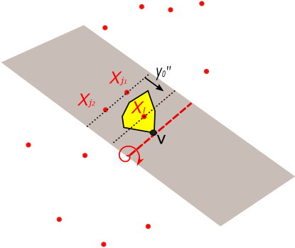
Figure 3: Shown is a 3-dimensional illustration for Theorem 2 if $X_{l}$ is an inner point of a 2-dimensional facet $\mathcal{F}$, i.e., the polygon on the separating hyperplane, of $\mathcal{M}$.

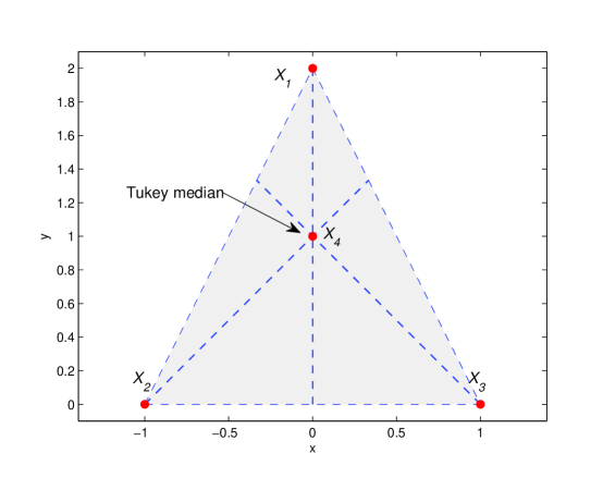
Figure 4: Shown is an example such that $\mathcal{M}$ contains only a single sample point, namely, $X_{4}$. Hence, $X_{4}$ can serve as the Tukey median.

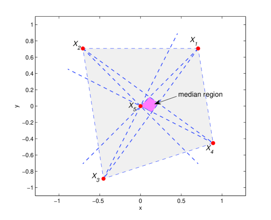
Figure 5: Shown is an example such that $\mathcal{M}$ is of affine dimension $p=2$.

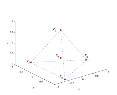
(a) Shown is an example such that $\mathcal{M}$ is singleton.

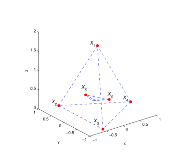
(b) Shown is an example such that $\mathcal{M}$ is of affine dimension $p=3$.

Figure 6: Shown are examples of $\mathcal{M}$ when $p=3$.

Unfortunately, the latter scenario is very much possible in practice in the sense that $\mathcal{M}$ contains more than a single point. As one can see from Figure 5, although $X_{5}$ is one of the points maximizing the Tukey depth, it can not be used as the Tukey median for the sake of affine equivariance and because the average of $\mathcal{M}$ should be in the interior of $\mathcal{M}$, while $X_{5}$ is on the boundary. (Two 3-dimensional examples of both scenarios are shown in Figure 6.)

So when $\mathcal{M}$ is a singleton? The following theorem partially answers this question.

Theorem 3. Suppose $\mathcal{X}^{n}$ is in general position. Then when $\lambda^{*}=\frac{\lfloor(n-p+2)/2\rfloor}{n}$ with $n>p\geq 2$, $\mathcal{M}$ contains only a single point.

Proof. In the sequel we will show that if $\textbf{dim}(\mathcal{M})>0$, it would lead to a contradiction under the current assumptions. We focus only on the scenario $\textbf{dim}(\mathcal{M})=1$. The proof of the rest cases follows a similar fashion.

When $\textbf{dim}(\mathcal{M})=1$, $\mathcal{M}$ is in fact a line segment. Denote $\textbf{\emph{x}}_{1}$, $\textbf{\emph{x}}_{2}$ to be its two endpoints. The compactness of $\mathcal{M}$ implies that, among $\{\textbf{\emph{u}}_{1}^{*},\textbf{\emph{u}}_{2}^{*},\cdots,\textbf{\emph{u}}_{m}^{*}\}$, there must exist a $\textbf{\emph{u}}_{j}^{*}$ such that

$$(\textbf{\emph{u}}_{j}^{*})^{\top}\textbf{\emph{x}}_{1}=q_{j}\text{ and }(\textbf{\emph{u}}_{j}^{*})^{\top}\textbf{\emph{x}}_{2}>q_{j}.$$ (15)

If not, all points x in the line $\ell$ that passes through $\textbf{\emph{x}}_{1}$ and $\textbf{\emph{x}}_{2}$ satisfy that $(\textbf{\emph{u}}_{k}^{*})^{\top}\textbf{\emph{x}}=q_{k}$, $k=1,2,\cdots,m$. This implies $\ell\subset\mathcal{M}$, contradicting with the boundedness of $\mathcal{M}$. On the other hand, by (2), there must exist $p$ observations, say $X_{i_{1}},X_{i_{2}},\cdots,X_{i_{p}}$, satisfying that $(\textbf{\emph{u}}^{*})^{\top}X_{i_{1}}=(\textbf{\emph{u}}^{*})^{\top}X_{i_{2}}=\cdots=(\textbf{\emph{u}}^{*})^{\top}X_{i_{p}}=(\textbf{\emph{u}}^{*})^{\top}\textbf{\emph{x}}_{1}$. (If $\textbf{\emph{x}}_{1}$ is a sample point, assume $X_{i_{1}}=\textbf{\emph{x}}_{1}$.) This, combined with (15), easily leads to

$$nP_{n}((-\textbf{\emph{u}}_{j}^{*})^{\top}X\leq(-\textbf{\emph{u}}_{j}^{*})^{\top}\textbf{\emph{x}}_{2})\leq\left\lfloor\frac{n-p}{2}\right\rfloor.$$

This contradicts with the fact $\textbf{\emph{x}}_{2}\in\mathcal{M}$. $\Box$

4 Concluding remarks

In the computing of Tukey’s halfspace median, the lower and upper bounds given in DG92 on the maximum halfspace depth are employed in the literature. The lower bound is sharp, but the upper bound is not in general (as shown in this paper), which could cause lots of unnecessary efforts in the searching of depth contours/regions. Computing of a singe depth contour can cost lots of time and effort. By providing a sharper and sharpest upper bound could save a lot of resource in practices, which is exactly achieved in this manuscript. Furthermore, we provide answers to the questions “Can a single deepest sample point serve as Tukey’s halfspace median? If yes, in what kind of situation?”.

Results established here are not only interesting themselves theoretically but useful practically as well. Furthermore, observe that the finite sample breakdown point (FSBP) of Tukey’s halfspace median $T^{*}$ is closely related to the maximum Tukey depth (Donoho and Gasko, 1992). We anticipate that they will be extremely helpful for establishing the FSBP of $T^{*}$ and revealing its impact from the dimensionality $p$. This is still an open problem up to this point, although similar discussions have been conducted for some other multivariate location estimators (Zuo et al., 2004; Müller, 2013).

References

- Bickel (1964) Bickel, P.J., 1964. On some alternative estimates for shift in the -variate one sample problem. The Annals of Mathematical Statistics, 35(3), 1079-1090.
- Brown (1983) Brown, B.M., 1983. Statistical use of the spatial median. Journal of the Royal Statistical Society. Series B 45, 25-30.
- Donoho and Gasko (1992) Donoho, D.L., Gasko, M., 1992. Breakdown properties of location estimates based on halfspace depth and projected outlyingness. Ann. Statist. 20, 1808-1827.
- Dyckerhoff and Mozharovskyi (2016) Dyckerhoff, R., Mozharovskyi, P., 2016. Exact computation of the halfspace depth. Comput. Statist. Data Anal., 98, 19-30.
- Hastie et al. (2008) Hastie, T., Tibshirani, R., Friedman, J. 2008. The elements of statistical learning: data mining, inference and prediction (2nd). Springer.
- Juan and Prieto (1995) Juan, J., Prieto, F.J. 1995. A subsampling method for the computation of multivariate estimators with high breakdown point. J. Comput. Graph. Statist. 4, 319-334.
- Lange et al. (2014) Lange, T., Mosler, K., Mozharovskyi, P. (2014). Fast nonparametric classification based on data depth. Statistical Papers, 55(1), 49-69.
- Liu (1990) Liu, R. Y., 1990. On a notion of data depth based on random simplices. Ann. Statist. 18, 191-219.
- Liu and Zuo (2014) Liu, X., Zuo, Y., 2014. Computing halfspace depth and regression depth. Communications in Statistics-Simulation and Computation, 43, 969-985.
- Miller et al. (2003) Miller, K., Ramaswami, S., Rousseeuw, P., Sellarès, J. A., Souvaine, D., Streinu, I., Struyf, A. 2003. Efficient computation of location depth contours by methods of computational geometry. Statistics and Computing, 13(2), 153-162.
- Mosler et al. (2009) Mosler, K., Lange, T., Bazovkin, P., 2009. Computing zonoid trimmed regions of dimension . Comput. Statist. Data Anal. 53, 2500-2510.
- Müller (2013) Müller, C., 2013. Upper and lower bounds for breakdown points. In: Becker, C., Fried, R., and Kuhnt, S. (eds.), Robustness and Complex Data Structures, Festschrift in Honour of Ursula Gather, Springer, Berlin, Heidelberg, 17-34.
- Paindaveine and Šiman (2011) Paindaveine, D., Šiman, M., 2011. On directional multiple-output quantile regression. J. Multivariate Anal. 102, 193-392.
- Paindaveine and Šiman (2012a) Paindaveine, D., Šiman, M., 2012a. Computing multiple-output regression quantile regions. Comput. Statist. Data Anal. 56, 840-853.
- Paindaveine and Šiman (2012b) Paindaveine, D., Šiman, M., 2012b. Computing multiple-output regression quantile regions from projection quantiles. Comput. Statist. 27, 29-49.
- Rousseeuw and Ruts (1998) Rousseeuw, P. J., Ruts, I. 1998. Constructing the bivariate Tukey median. Statistica Sinica, 8(3), 827-839
- Ruts and Rousseeuw (1996) Ruts, I., Rousseeuw, P.J., 1996. Computing depth contours of bivariate point clouds. Comput. Statist. Data Anal. 23, 153-168.
- Small (1990) Small, G. (1990). A survey of multidimensional medians. Int. Statist. Rev., 58, 263-277.
- Struyf and Rousseeuw (2000) Struyf, A., Rousseeuw, P. J. (2000). High-dimensional computation of the deepest location. Comput. Statist. Data Anal., 34(4), 415-426.
- Tukey (1975) Tukey, J.W., 1975. Mathematics and the picturing of data. In Proceedings of the International Congress of Mathematicians, 523-531. Cana. Math. Congress, Montreal.
- Weber (1909) Weber, A. (1909). Uber den Standort der Industrien, Tubingen. English translation by Freidrich, C. J. (1929), Alfred Weber’s Theory of Location of Industries, University of Chicago Press.
- Zuo (2004) Zuo, Y. 2004. Projection-based affine equivariant multivariate location estimators with the best possible finite sample breakdown point. Statistica Sinica, 14(4), 1199-1208.
- Zuo et al. (2004) Zuo, Y.J., Cui, H.J., He, X.M., 2004. On the Stahel-Donoho estimators and depth-weighted means for multivariate data. Ann. Statist. 32, 189-218.
- Zuo and Serfling (2000a) Zuo, Y.J., Serfling, R., 2000a. General notions of statistical depth function. Ann. Statist. 28, 461-482.
- Zuo and Serfling (2000) Zuo, Y.J., Serfling, R., 2000. On the performance of some robust nonparametric location measures relative to a general notion of multivariate symmetry. Journal of Statistical Planning and Inference, 84(1), 55-79.