Jansen-MIDAS: a multi-level photomicrograph segmentation software based on isotropic undecimated wavelets

Abstract

Image segmentation, the process of separating the elements within an image, is frequently used for obtaining information from photomicrographs. However, segmentation methods should be used with reservations: incorrect segmentation can mislead when interpreting regions of interest (ROI), thus decreasing the success rate of additional procedures. Multi-Level Starlet Segmentation (MLSS) and Multi-Level Starlet Optimal Segmentation (MLSOS) were developed to address the photomicrograph segmentation deficiency on general tools. These methods gave rise to Jansen-MIDAS, an open-source software which a scientist can use to obtain a multi-level threshold segmentation of his/hers photomicrographs. This software is presented in two versions: a text-based version, for GNU Octave, and a graphical user interface (GUI) version, for MathWorks MATLAB. It can be used to process several types of images, becoming a reliable alternative to the scientist.

Keywords: GNU Octave, Image Processing, MATLAB, Microscopy, Segmentation, Wavelets

1 Introduction

Microscopy plays a key role in addressing several issues in biology [1, 2], materials science [3, 4], geology [5], among other areas. Nowadays, image processing techniques are frequently used together with microscopy, helping scientists to analyze photomicrographs of different samples. For instance, image segmentation can be used to separate elements within a photomicrograph, conducting the scientist to obtain relevant information such as counting objects in a sample, or determining their area.

There are a considerable number of computational packages available for segmentation. One of the most known ones is the open source project Fiji [6], a tool based on ImageJ [7] and aimed primarily at life sciences. Also, there are several methods rising for segmentation of different photomicrographs, obtained by confocal [8], magnetic resonance [9], and transmission electron [10] microscopies.

Despite the satisfactory segmentation which general methods present on different images, more specific ones should be used with reservations as they can return poor results when analyzing objects different from their original specifications. In addition, incorrect segmentation can mislead when interpreting regions of interest (ROI), thus decreasing the success rate of additional computational procedures.

To address the issues on photomicrograph segmentation using general methods, the algorithms named Multi-Level Starlet Segmentation (MLSS) [11] and Multi-Level Starlet Optimal Segmentation (MLSOS) [12] were developed. These methods gave rise to the open-source software Jansen-MIDAS, available at [13], which a scientist can use to obtain a multi-level threshold segmentation of his/hers photomicrograph, besides using supervised learning based on the comparison between the photomicrograph ground truth and the Matthews correlation coefficient (MCC) [14] to obtain the optimal segmentation between all levels. Jansen-MIDAS was used previously for separating elements of two different materials, gold nanoparticles reduced on natural rubber membranes [11] and fission tracks on the surface of epidote crystals [12], returning an accuracy higher than 89 % in these applications.

This article is given as follows. Section 2 presents a brief introduction on starlet wavelet transform, Multi-Level Starlet Segmentation (MLSS) and Multi-Level Starlet Optimal Segmentation (MLSOS) algorithms, and Matthews correlation coefficient (MCC), the techniques implemented in Jansen-MIDAS. Next, the Section 3 describes the two versions (text-based and graphical user interface) of this software, and presents examples of their utilization. On Section 4, we discuss the use of Jansen-MIDAS on the previous applications. Finally, in the Section 5, we present our final considerations about this study.

2 Methods

Jansen-MIDAS allows the user to apply the Multi-Level Starlet Segmentation (MLSS), a multi-level segmentation method based on starlet wavelets, and aimed to separate elements in photomicrographs. Combining MLSS and the Matthews correlation coefficient (MCC), we developed the Multi-Level Starlet Optimal Segmentation (MLSOS), an optimal segmentation tool. These methods are described in this section.

2.1 The starlet wavelet

The starlet wavelet is an isotropic and undecimated transform, suited to the analysis of images which contains isotropic structures (e.g. astronomic [15] or biological ones [16]), and also for structure denoising (e.g. three-dimensional electron tomographies [17]).

The two-dimensional starlet wavelet is obtained from the scale $\phi$ and wavelet $\psi$ functions [18, 19]:

$$\phi_{1D} = \frac{1}{12}\left(|t-2|^{3}-4|t-1|^{3}+6|t|^{3}-4|t+1|^{3}+|t+2|^{3}\right)$$

$$\phi(t_{1},t_{2}) = \phi_{1D}(t_{1})\phi_{1D}(t_{2})$$ (1)

$$\frac{1}{4}\psi\left(\frac{t_{1}}{2},\frac{t_{2}}{2}\right) = \phi(t_{1},t_{2})-\frac{1}{4}\phi\left(\frac{t_{1}}{2},\frac{t_{2}}{2}\right)$$ (2)

where $\phi_{1D}$ is the one-dimensional third order B-spline ($B_{3}$-spline), a smooth function capable of separating large structures within an image [20]. The wavelet function $\psi$, in its turn, is obtained from the difference between two decomposition levels.

Similarly to Equations 1 and 2, the finite impulse response (FIR) filters $(h,g)$ related to the starlet wavelet are defined by [20]:

$$h_{1D} = \frac{[\begin{array}[]{ccccc}1&4&6&4&1\\ \end{array}]}{16}$$ (4)

$$h[k,l] = h_{1D}[k]h_{1D}[l]$$ (5)

$$g[k,l] = \delta[k,l]-h[k,l]$$ (6)

where $k,l=-2,...,2$, and $\delta$ is defined as $\delta[0,0]=1$ and $\delta[k,l]=0$ for all $[k,l]\neq(0,0)$. One can obtain the detail wavelet coefficients from the difference between current and previous decomposition levels, as in Equations 2 and 6.

Using Equation 5, the two-dimensional starlet application begins with a convolution between the input image $c_{0}$ and $h$ (Equation 7):

$$h=\frac{1}{16}\left[\begin{array}[]{c}1\\ 4\\ 6\\ 4\\ 1\end{array}\right]*\frac{1}{16}\left[\begin{array}[]{ccccc}1&4&6&4&1\end{array}\right]=\left[\begin{array}[]{ccccc}\frac{1}{256}&\frac{1}{64}&\frac{3}{128}&\frac{1}{64}&\frac{1}{256}\\ \frac{1}{64}&\frac{1}{16}&\frac{3}{32}&\frac{1}{16}&\frac{1}{64}\\ \frac{3}{128}&\frac{3}{32}&\frac{9}{64}&\frac{3}{32}&\frac{3}{128}\\ \frac{1}{64}&\frac{1}{16}&\frac{3}{32}&\frac{1}{16}&\frac{1}{64}\\ \frac{1}{256}&\frac{1}{64}&\frac{3}{128}&\frac{1}{64}&\frac{1}{256}\end{array}\right]$$ (7)

This convolution returns a set of smooth coefficients corresponding to the first starlet decomposition level, $c_{1}$. Then, the wavelet detail coefficients for this level, $w_{1}$, are obtained from the difference $c_{0}-c_{1}$, as discussed earlier.

Let $L$ be the last desired decomposition level. Therefore, one can calculate the decomposition levels by:

$$c_{j}=c_{j-1}*h,$$

$$w_{j}=c_{j-1}-c_{j},$$

where $j=0,\ldots,L$ and $*$ is the convolution operator (Figure 1).

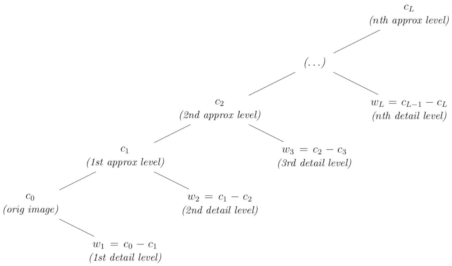
Figure 1: Tree representing the starlet decomposition structure. The starlet detail level $w_{i}$ is obtained by subtracting the approximation levels $c_{i}$ and $c_{i+1}$.

For $j>1$, $h$ has $2^{j}-1$ zeros between its elements [21]. These operations generate a set $W=\{w_{1},\ldots,w_{L},c_{L}\}$, which is the starlet decomposition of the input image $c_{0}$.

2.2 Multi-Level Starlet Segmentation (MLSS)

The method used in Jansen-MIDAS for photomicrograph segmentation is denominated Multi-Level Starlet Segmentation (MLSS). It is based on the starlet wavelet, and provides the multi-level photomicrograph segmentation. There are two alternatives for applying MLSS: the original and derivative algorithms.

2.2.1 Original MLSS algorithm

The original MLSS algorithm is based on the addition of detail levels obtained from starlet application. After obtaining the sum of the detail levels, the input image $c_{0}$ is subtracted, in order to reduce background noise. This version is implemented as follows:

• The user chooses $L$, the last desired decomposition level. The starlet transform is applied to the input image $c_{0}$, resulting in $L$ wavelet detail decomposition levels: $w_{1},\cdots,w_{L}$.

• After obtaining the detail levels, the user chooses the initial detail level to be used in the sum, $L_{0}$. Detail levels lower than $L_{0}$ ($w_{1},\cdots,w_{L_{0}-1}$) are ignored in this approach; this strategy can be useful for removing noise from the input image, which usually remains within the first decomposition levels.

• Then, the detail levels $L_{0}$ to $i$ are summed, and $c_{0}$ is subtracted from the result:

  $$R_{i}=\sum_{k=L_{0}}^{i}w_{k}-c_{0},\,L_{0}\leq i\leq L,$$

  where $R_{i}$ is the starlet-related segmentation for its decomposition level $i$.

This algorithm results in $R_{w}=\{R_{L_{0}},R_{L_{0}+1},\cdots,R_{L}$}, a matrix with $L-L_{0}$ segmentation levels. Each level $R_{i}$ corresponds to the starlet detail level $w_{i}$, and then the user can choose the best segmentation level for the input image.

2.2.2 Derivative MLSS algorithm

The derivative MLSS algorithm also uses the starlet detail decomposition levels, following the same basis of the original algorithm. However, there is no subtraction of the input image, in order to preserve possible small regions of interest (ROI). Its implementation follows:

• The starlet transform is applied on the input image $c_{0}$, generating $L$ detail levels: $w_{1},\cdots,w_{L}$, where $L$ is the last decomposition level.

• The user chooses the initial detail level, $L_{0}$. Detail levels lower than $L_{0}$ ($w_{1},\cdots,w_{L_{0}-1}$) are ignored, and $w_{L_{0}},\cdots,w_{j}$ are summed:

  $$R_{i}=\sum_{k=L_{0}}^{i}w_{k},\,L_{0}\leq i\leq L,$$

  where $R_{i}$ is the starlet-related segmentation for its decomposition level $i$.

Similarly, the algorithm returns $R_{w}=\{R_{L_{0}},R_{L_{0}+1},\cdots,R_{L}$}. The segmentation level $R_{i}$ corresponds to the starlet detail level $w_{i}$, and the user can choose the best segmentation level for the input image.

2.2.3 Matthews correlation coefficient (MCC)

Regions of interest (ROI) in an input image can be represented in a binary image denominated ground truth (GT). Generally, the GT is obtained by an expert, which indicates the ROI and the background on the input image. Then, the GT can be generated representing the ROI and the background using two different colors (usually, white and black).

One can compare the segmentation of an input image given by an algorithm with its GT, in order to estimate the success rate of this segmentation. From this comparison, we can define the resulting pixels as true positives (TP), true negatives (TN), false positives (FP) and false negatives (FN), where:

• TP: pixels correctly labeled as ROI by the algorithm.

• FP: pixels incorrectly labeled as ROI by the algorithm.

• FN: pixels incorrectly labeled as background by the algorithm.

• TN: pixels correctly labeled as background by the algorithm.

From TP, TN, FP and FN, one can quantify the quality of the segmentation using the Matthews correlation coefficient (MCC) [14]:

$$\mathcal{M}=\frac{TP*TN-FP*FN}{\sqrt{(TP+FN)(TP+FP)(TN+FP)(TN+FN)}}\times 100\%,$$ (8)

where $\mathcal{M}\in[-100\%,100\%]$.

Higher $\mathcal{M}$ values indicate satisfactory segmentation: $100\%$, zero and $-100\%$ represent perfect, random and opposite segmentations, respectively [22].

2.2.4 Multi-Level Starlet Optimal Segmentation (MLSOS)

In this section we present the extension of MLSS. It employs the Matthews correlation coefficient (MCC, Equation 8) to obtain the optimal segmentation level. The refined method is named Multi-Level Starlet Optimal Segmentation (MLSOS), and is defined as follows [12, 23]:

• MLSS is applied in a input image $c_{0}$ that has its GT for $L$ desired starlet decomposition levels, thus acquiring $R_{w}=\{R_{L_{0}},R_{L_{0}+1},\cdots,R_{L}\}$.

• The segmentation results for each starlet level, $R_{i}$, with $i=L_{0},\cdots,L$, are compared with the GT of the input image, thereby obtaining TP_i, TN_i, FP_i and FN_i.

• Based on these values, MCC is calculated for each $R_{i}$.

Therefore, the optimal segmentation level obtained for the input photomicrograph is the one which returns the higher MCC value between segmentation levels $R_{i},L_{0}\leq i\leq L$ obtained by MLSS.

Using MLSOS, one can establish the optimal segmentation level for the photomicrographs of a sample representing the set, thus estimating the optimal level for the entire photomicrograph set.

3 Jansen-MIDAS description and operating instructions

The software Jansen-MIDAS contains implementations for the MLSS and MLSOS methods. Using this software, scientists can apply these techniques on their own photomicrographs.

There are two versions of Jansen-MIDAS: one is based on text input, built for GNU Octave, and another has a graphical user interface (GUI), aimed to MATLAB users. They are distributed in the same package, in the folders TEXTMODE and GUIMODE, containing the text-based version and the GUI version respectively. On the next section, we describe both versions and how to use them.

3.1 Text-based version

Using Jansen-MIDAS’s text-based version is straightforward. After starting GNU Octave, it presents its GUI containing the Command Window and its prompt, represented by two “greater than or equal” symbols (>>). If Octave is running from the TEXTMODE folder, Jansen-MIDAS is started typing the following command in the Command Window:

>> jansenmidas();

Alternatively, the user can inform the variables which will store the processing results on Octave. This can be done using the following command, which starts Jansen-MIDAS and stores the processing results on the variables D, R, COMP and MCC:

>> [D,R,COMP,MCC] = jansenmidas();

These variables represent:

• D: the starlet detail decomposition levels.

• R: the MLSS segmentation levels.

• COMP: a color comparison between the input photomicrograph and its GT, representing TP, FP, and FN pixels.

• MCC: the Matthews correlation coefficient values for each segmentation level.

An example of applying the text-based version follows. First, the software presents itself:

%%%%%%%%%%%%%%%%%%%%%%%%%%%%%%%%%%%%%%%%%%%%%%%%%%%%%%%%
%%%%%%%%%%%%%%% Welcome to Jansen-MIDAS %%%%%%%%%%%%%%%%
%%%%%%%%%% Microscopic Data Analysis Software %%%%%%%%%%
%%%%%%%%%%%%%%%%%%%%%%%%%%%%%%%%%%%%%%%%%%%%%%%%%%%%%%%%

The first step is to provide the first starlet detail level to be considered on the segmentation. If the user enters $3$, for example, the starlet detail levels $1$ and $2$ will be disregarded from the segmentation. Remind that lower and higher detail levels present smaller and larger detail ROI, respectively.

Initial detail level to consider in segmentation:

In this example we suppose the user does not input a first detail level. When this happens, Jansen-MIDAS assumes this value as $1$:

Assuming default value, initial level equals 1. Continue...

After that, the software asks the last desired segmentation level.

Last detail level to consider in segmentation:

Similarly to when choosing the first level, if the user does not input the last segmentation, the software assumes the default value, $5$. In this example, we consider the last segmentation level equals to $3$:

Last detail level to consider in segmentation: 3

Now Jansen-MIDAS asks the name of the photomicrograph to be processed. The TEXTMODE folder contains two test images, named test1.jpg and test2.jpg (Figure 2). These images are suitable to test the original and derivative MLSS algorithms, respectively.

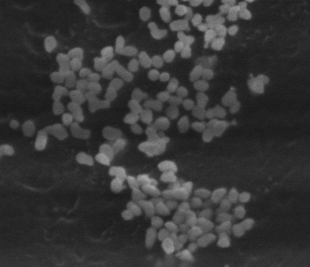
(a) Figure test1.jpg, suitable for testing the original MLSS.

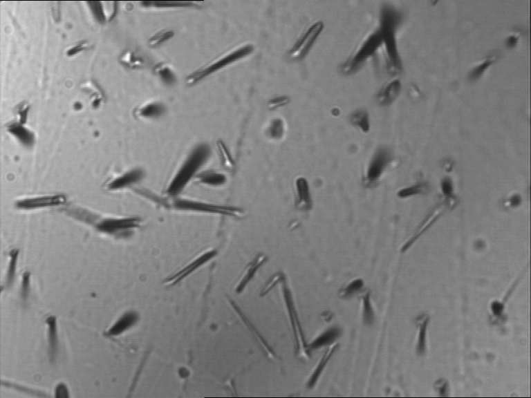
(b) Figure test2.jpg, suitable for testing the derivative MLSS.

Figure 2: Test images provided with Jansen-MIDAS. These pictures are suitable for testing both original and derivative MLSS algorithms.

Please type the original image name:

For this example, we chose the image test1.jpg. Then, the software performs the MLSS on it, asking before what processing algorithm to use (original or derivative).

Applying MLSS...
Type V for Variant or any to Original MLSS:

In order to use the derivative algorithm, the user will type v or V. However, the original algorithm is the suitable one for the photomicrograph test1.jpg. To apply it, simply press Enter.

After that, the software asks if it will apply MLSOS on the photomicrograph; if yes, it is sufficient to type y or Y. In order to do that, the user should have the GT image representing the ROI on the input photomicrograph, thus Jansen-MIDAS will estimate the MCC values for each segmentation and generate the comparison between input image and GT.

Do you want to apply MLSOS (uses GT image)?
Please type a GT image name:

The folder TEXTMODE contains also the GT images of the test photomicrographs. The file names are test1GT.jpg and test2GT.jpg (Figure 3). Since we chose test1.jpg, test1GT.jpg is the GT image to be used on the comparison.

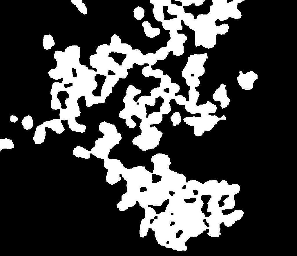
(a) Figure test1GT.jpg, GT image of Figure 2a.

(b) Figure test2GT.jpg, GT image of Figure 2b.

Figure 3: Ground truth (GT) of the test photomicrographs text1.jpg and text2.jpg, also provided with the software Jansen-MIDAS. Together with their respective original images, the GT are used to apply MLSOS.

When MLSOS application finishes, the values of MCC for each segmentation level are shown on a plot (Figure 4). Then the program asks if it should record the resulting images or only display them.

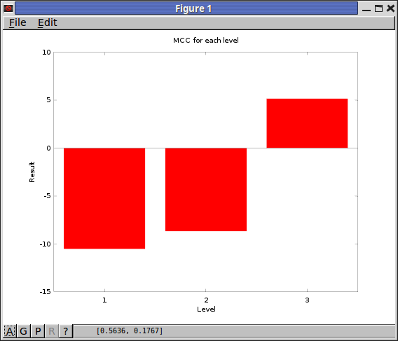
Figure 4: The Matthews correlation coefficient plot presented by Jansen-MIDAS’s text-based version, using test1.jpg and test1GT.jpg. First and last segmentation levels equal to $1$ and $3$, respectively.

Type Y to save images or any to show them:

If the user enters y or Y, the images will be stored with the same name of the original image, and information about the results, in three groups:

1. D, representing the starlet detail decomposition levels;

2. R, representing the MLSS segmentation levels;

3. COMP, representing the comparison between the input photomicrograph and its GT, when the last is provided.

For first and last levels equal to $1$ and $3$, the information presented on the screen is:

Saving detail image... Level: 1
Saving detail image... Level: 2
Saving detail image... Level: 3
Saving segmentation image... Level: 1
Saving segmentation image... Level: 2
Saving segmentation image... Level: 3
Saving comparison image... Level: 1
Saving comparison image... Level: 2
Saving comparison image... Level: 3

When the user chooses to not store the images, the results are presented directly on the screen (Figure 5). For first and last starlet detail levels equal to $1$ and $3$, the presented information follows:

Showing detail image... Level: 1
Showing detail image... Level: 2
Showing detail image... Level: 3
Showing segmentation image... Level: 1
Showing segmentation image... Level: 2
Showing segmentation image... Level: 3
Showing comparison image... Level: 1
Showing comparison image... Level: 2
Showing comparison image... Level: 3

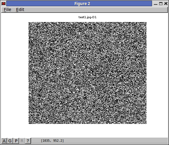
(a) Window D1.

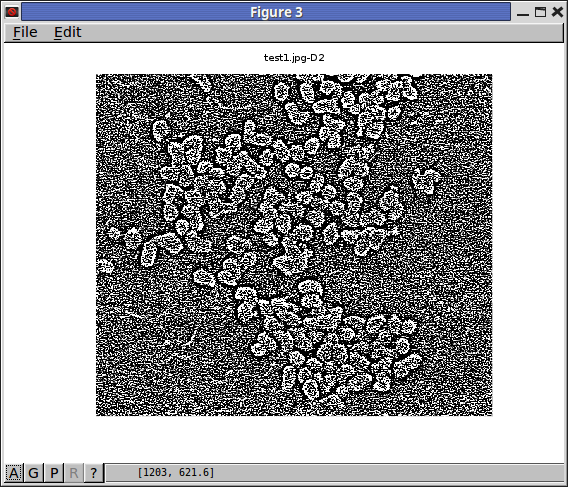
(b) Window D2.

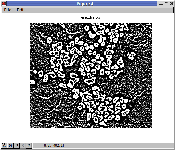
(c) Window D3.

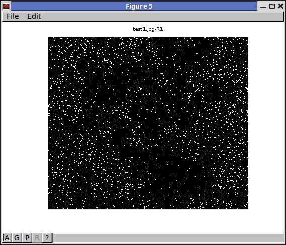
(d) Window R1.

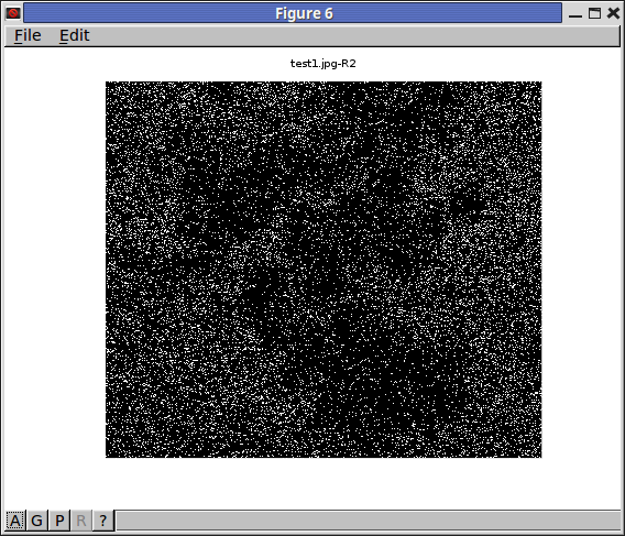
(e) Window R2.

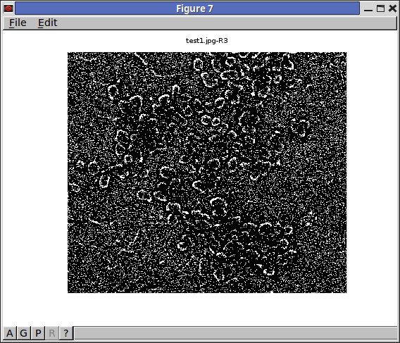
(f) Window R3.

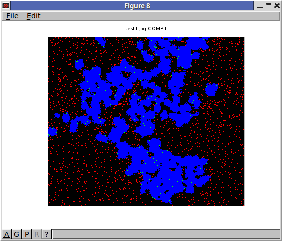
(g) Window COMP1.

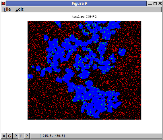
(h) Window COMP2.

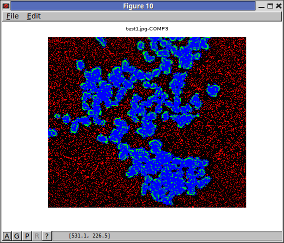
(i) Window COMP3.

Figure 5: Windows presenting Jansen-MIDAS’s application results on the text-based version, using test1.jpg and test1GT.jpg. The application of MLSOS returns three image sets: detail (D), segmentation (R) e comparison (COMP). The segmentation levels are $1$ (first) and $3$ (last), generating three images on each set.

Finally, Jansen-MIDAS processing ends with the following final message:

End of processing. Thanks!

3.2 Graphical user interface version

Jansen-MIDAS’s graphical version is also easy to use, although it is not straightforward as the text-based version. This version has interactive elements such as buttons, check and text boxes.

As in GNU Octave, the MATLAB environment has several areas. Its prompt is also available on the Command Window and represented by >>. Inside the folder GUIMODE, Jansen-MIDAS starts when typing the following command in MATLAB:

>> JansenMIDAS

Then the initial screen is presented (Figure 6). The first elements presented are:

• The state button MLSOS (with GT). When pressed, the software will apply MLSOS besides MLSS.

• The text boxes First dec level and Last dec level, where the user can inform to Jansen-MIDAS what are the first and the last segmentation levels to use.

• The check box Variation algorithm. When checked, the software applies the derivative MLSS algorithm.

• The check boxes Show D and Show R. When checked, Jansen-MIDAS will present the starlet detail levels and segmentation results instead of storing them on the disk.

• The welcome text Welcome to Jansen-MIDAS, which presents information on the processing as the software performs its tasks.

• The button Open image…, which asks the input image, to the user, thus starting the processing.

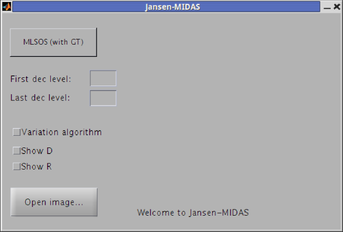
Figure 6: Jansen-MIDAS’s graphical user interface (GUI), developed for MathWorks MATLAB.

One example of Jansen-MIDAS’s application using the GUI version is given below. The processing starts when the user clicks on the button Open image…. Then, a window asks the input photomicrograph. The GUIMODE folder also contains the test images test1.jpg and test2.jpg, which can be used to simulate the software usage (Figure 2).

In this example we suppose the chosen photomicrograph is test2.jpg. The welcome text indicates the performing action, being changed to Opening image…. Then, the software shows the input image and the button Open image… becomes Process… (Figure 7).

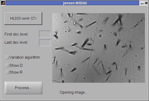
Figure 7: Jansen-MIDAS presenting the image to be segmented. After choosing the input photomicrograph, the button Open image… becomes Process…, and the welcome text is changed to Opening image….

At this point the user can choose other options:

• If MLSOS will be used, pressing the button MLSOS (with GT).

• The first and last segmentation levels, on the text boxes First dec level and Last dec level. As in Jansen-MIDAS’s text version, the default first and last segmentation levels, assumed when these boxes do not receive values, are $1$ and $5$ respectively.

• If the software will present the starlet detail levels and segmentation results on the screen, using the check boxes Show D and Show R.

The derivative MLSS algorithm is suited to segment test2.jpg. Thus, if the user would want to apply MLSOS, with first and last segmentation levels equal to $1$ and $3$, derivative MLSS algorithm and showing starlet details (D) and segmentation results (R), the options on the software interface would be filled as in Figure 8

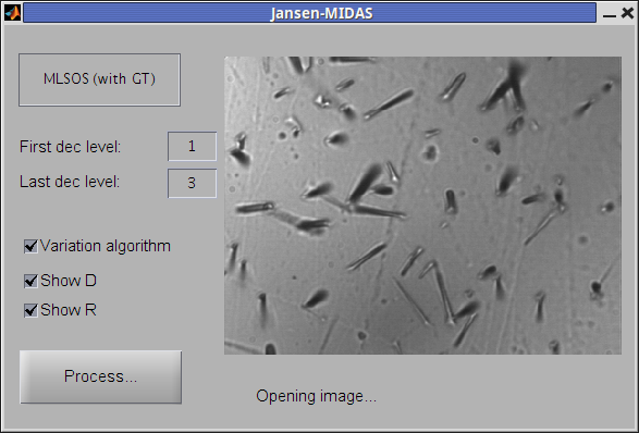
Figure 8: Jansen-MIDAS’s GUI interface corresponding to applying MLSOS, first and last segmentation levels equal to $1$ and $3$ respectively, using the derivative MLSS algorithm and presenting starlet detail levels (D) and segmentation results (R).

After choosing the desired options, the processing starts when the button Process… is pressed. In this example the user pressed the state button MLSOS (with GT); therefore, Jansen-MIDAS asks the GT image corresponding to the input photomicrograph. The folder GUIMODE also contains the GT images of the test photomicrographs, test1GT.jpg and test2GT.jpg (Figure 3). The GT image test2GT.jpg is used to apply MLSOS on test2.jpg.

When the user inputs the GT image, the software presents it and the segmentation starts. Then Jansen-MIDAS shows a window containing MCC values for each segmentation (Figure 9) and the windows presenting D, R and COMP, according to the user’s choices (Figure 10).

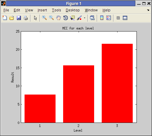
Figure 9: Matthews correlation coefficient presented by Jansen-MIDAS’s application, GUI mode, using test2.jpg and test2GT.jpg. First and last segmentation levels equal to $1$ and $3$ respectively.

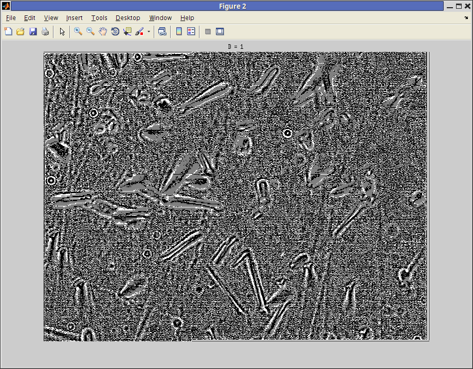
(a) Window D1.

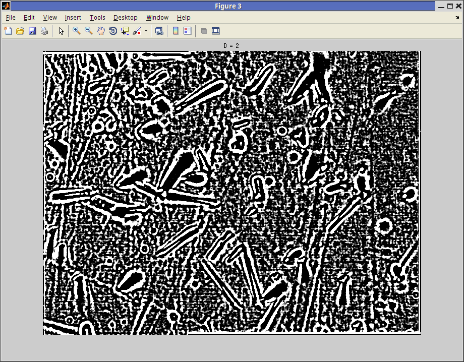
(b) Window D2.

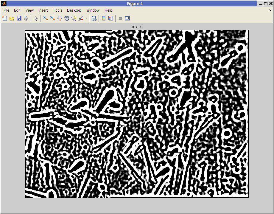
(c) Window D3.

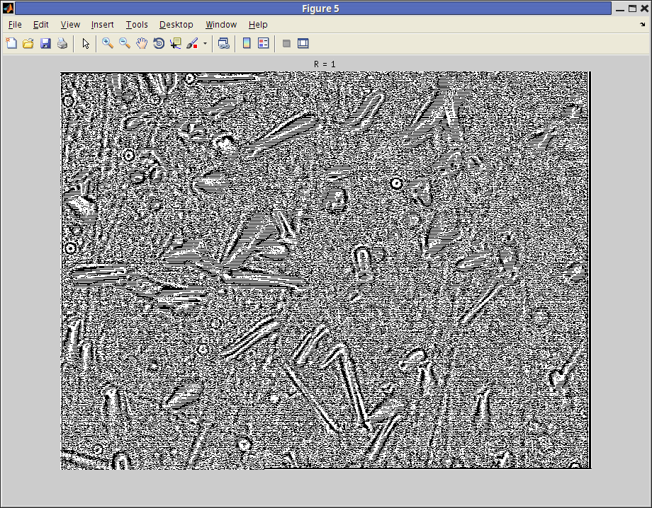
(d) Window R1.

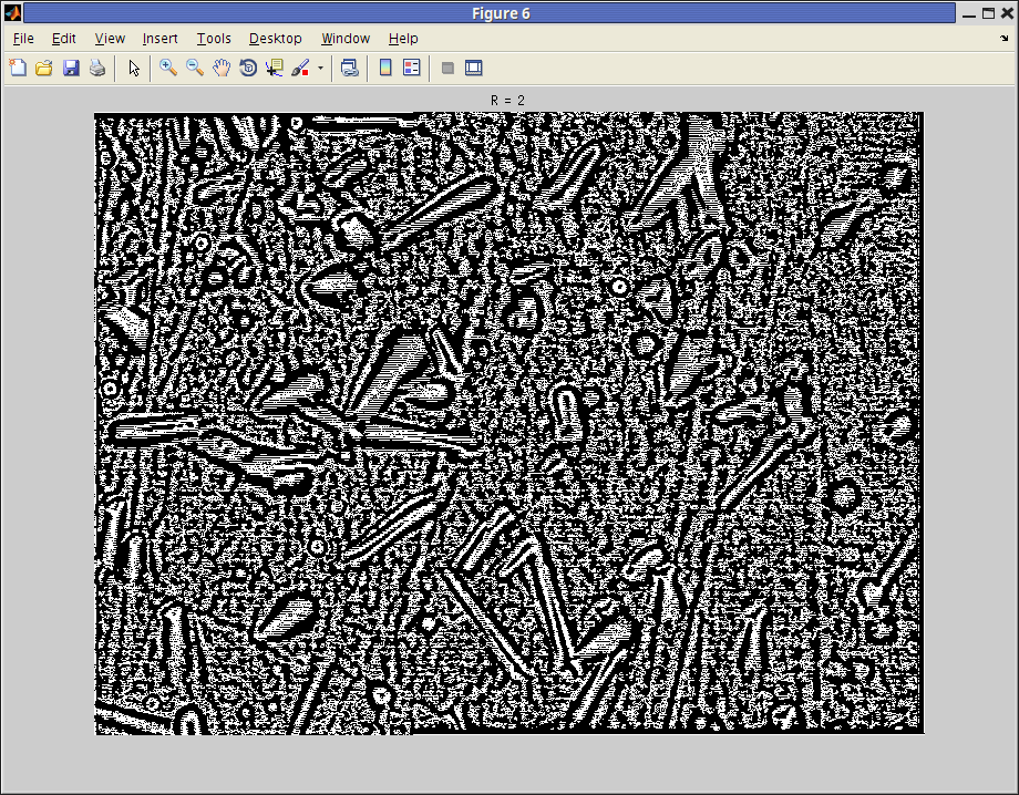
(e) Window R2.

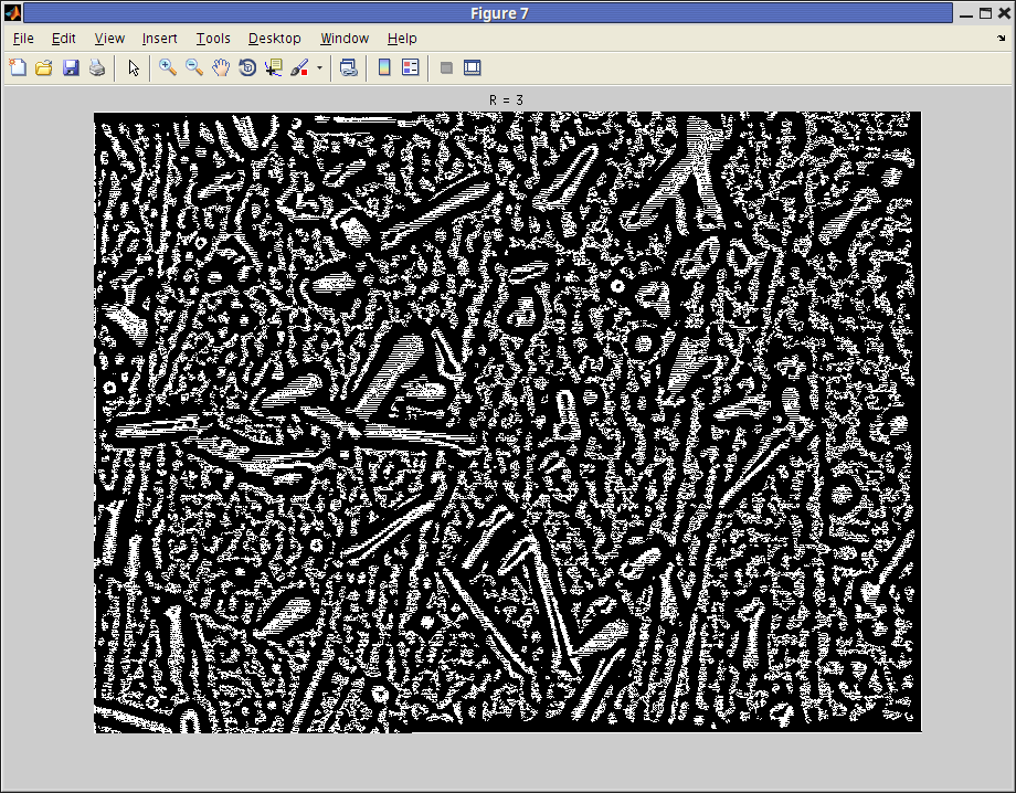
(f) Window R3.

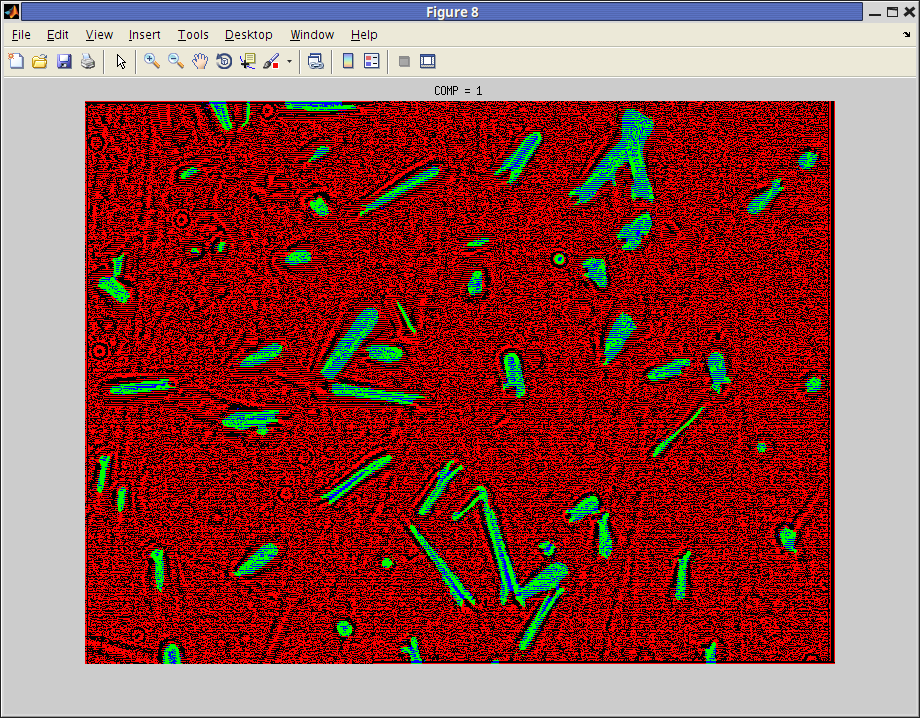
(g) Window COMP1.

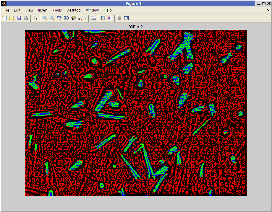
(h) Window COMP2.

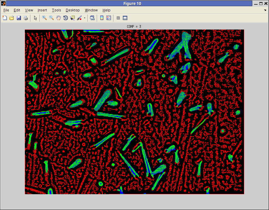
(i) Window COMP3.

Figure 10: Windows presenting Jansen-MIDAS’s application results on the GUI version, using test2.jpg and test2GT.jpg. The MLSOS application returns three image sets: details (D), segmentation (R) and comparison (COMP). The segmentation levels are $1$ (first) and $3$ (last), returning three images in each set.

In this example, the check boxes Show D and Show R were checked. Therefore, Jansen-MIDAS returns the image sets of starlet detail levels (D) and MLSS results (R). When MLSOS is applied, the images referring to the comparison between MLSS results and the GT corresponding to the input photomicrograph (COMP) is presented automatically. These results can be stored using the Save menu or button on each window. When the software ends its processing, the welcome text changes its information to Done.

4 Discussion

Most of the segmentation methods demand human intervention at some point of their execution. For example, the user of [24] needs to select between 60 and 70 % of well-binarized cells, and then the method continues the processing. Also, [25] uses texture-based features for providing a coarse segmentation of dendritic structures from C. elegans, which is improved after by post-processing.

Automatic segmentation methods benefit their users, which employ less effort on image processing. Besides, multi-level segmentation methods based on isotropic undecimated wavelets may enhance the segmentation process by offering a set of detail coefficients for each wavelet decomposition level. Based on these ideas, the algorithms implemented in Jansen-MIDAS were used previously on the study of two different materials:

Gold nanoparticles reduced on natural rubber membranes. The original MLSS algorithm implemented in Jansen-MIDAS was used for separating gold nanoparticles in scanning electron microscopy (SEM) photomicrographs reduced on natural rubber membranes [11], thus being able to estimate the amount of synthesized gold nanoparticles contained on the surface of these samples [23]. The amount of nanoparticles within a sample can be estimated combining Mie’s theory and ultraviolet-visible spectroscopy [26], a laborious approach. Moreover, it is difficult to define the stoichiometry and necessary parameters to estimate the density, i.e. the concentration/distribution of synthesized nanoparticles over a substrate, of organic substances developed using green chemistry.

Fission tracks on the surface of epidote crystals. The derivative MLSS algorithm implemented in Jansen-MIDAS was used for separating fission tracks in photomicrographs obtained from the surface of epidote crystals [12], which contain small ROI. Usually these tracks are counted manually on an optical microscope. There are commercial systems which perform this operation; for example, [27] describes an automatic method for counting fission tracks, based in two photomicrographs obtained from transmitted and reflected lights. These images are binarized and their intersection generates a coincidence mapping, which is used for the track analysis. A commercial system based on this method is available; however, the results acquired using this system often needs to be manually adjusted by the operator, being more time consuming than the usual measure [28]. Jansen-MIDAS’s application on the surface of epidote crystals had an accuracy higher than 89 %, and our approach can be extended to be an open alternative to these systems.

5 Conclusion

In this article we presented Jansen-MIDAS, a software developed to provide Multi-Level Starlet Segmentation (MLSS) and Multi-Level Starlet Optimal Segmentation (MLSOS) techniques. These methods are based on the starlet transform, an isotropic undecimated wavelet, in order to determine the location of objects in photomicrographs.

MLSS uses the addition of detail levels obtained from applying the starlet transform. There are two possible algorithms for MLSS: the input image may be subtracted (original algorithm) or not (derivative algorithm) from the sum of the detail coefficients. MLSOS, in its turn, chooses the optimal segmentation level from MLSS based on the Matthews correlation coefficient (MCC), which establishes the comparison between the set of training images and their ground truths.

Jansen-MIDAS is an open-source software released under the GNU General Public License. Its previous versions were used in the study of two different materials, returning an accuracy higher than 89 % in both applications. Jansen-MIDAS is presented in two versions: a text-based version, available for GNU Octave, and a graphical user interface (GUI) version, compatible with MathWorks MATLAB, which can be employed on the segmentation of several types of images, becoming a reliable alternative to the scientist.

References

References

- [1] T. A. Oliveira, G. Koakoski, A. C. da Motta, A. L. Piato, R. E. Barreto, G. L. Volpato, and L. J. G. Barcellos, “Death-associated odors induce stress in zebrafish,” Hormones and Behavior, vol. 65, no. 4, pp. 340 – 344, 2014.
- [2] S. Herculano-Houzel, C. S. von Bartheld, D. J. Miller, and J. H. Kaas, “How to count cells: the advantages and disadvantages of the isotropic fractionator compared with stereology,” Cell and tissue research, vol. 360, no. 1, pp. 29–42, 2015.
- [3] K. Henzler, A. Heilemann, J. Kneer, P. Guttmann, H. Jia, E. Bartsch, Y. Lu, and S. Palzer, “Investigation of reactions between trace gases and functional cuo nanospheres and octahedrons using nexafs-txm imaging,” Scientific Reports, vol. 5, no. 17729, pp. 1–12, 2015.
- [4] Y. Deng, A. Ediriwickrema, F. Yang, J. Lewis, M. Girardi, and W. M. Saltzman, “A sunblock based on bioadhesive nanoparticles,” Nature Materials, vol. 14, no. 12, pp. 1278–1285, 2015.
- [5] C. E. G. de Araujo, D. Rubatto, J. Hermann, U. G. Cordani, R. Caby, and M. A. Basei, “Ediacaran 2,500-km-long synchronous deep continental subduction in the west gondwana orogen,” Nature Communications, vol. 5, no. 5198, pp. 1–8, 2014.
- [6] J. Schindelin, I. Arganda-Carreras, E. Frise, V. Kaynig, M. Longair, T. Pietzsch, S. Preibisch, C. Rueden, S. Saalfeld, B. Schmid, et al., “Fiji: an open-source platform for biological-image analysis,” Nature methods, vol. 9, no. 7, pp. 676–682, 2012.
- [7] C. A. Schneider, W. S. Rasband, K. W. Eliceiri, et al., “Nih image to imagej: 25 years of image analysis,” Nature Methods, vol. 9, no. 7, pp. 671–675, 2012.
- [8] D. Sui and K. Wang, “A counting method for density packed cells based on sliding band filter image enhancement,” Journal of Microscopy, vol. 250, pp. 42–49, Apr. 2013.
- [9] L. Lin, S. Wu, and C. Yang, “A template-based automatic skull-stripping approach for mouse brain MR microscopy,” Microscopy Research and Technique, vol. 76, pp. 7–11, Jan. 2013.
- [10] P.-J. D. Temmerman, E. Verleysen, J. Lammertyn, and J. Mast, “Semi-automatic size measurement of primary particles in aggregated nanomaterials by transmission electron microscopy,” Powder Technology, vol. 261, no. 0, pp. 191 – 200, 2014.
- [11] A. F. de Siqueira, F. C. Cabrera, A. Pagamisse, and A. E. Job, “Segmentation of scanning electron microscopy images from natural rubber samples with gold nanoparticles using starlet wavelets,” Microscopy Research and Technique, vol. 77, pp. 71–78, jan 2014.
- [12] A. F. de Siqueira, W. Nakasuga, A. Pagamisse, C. A. Tello, and A. E. Job, “An automatic method for segmentation of fission tracks in epidote crystal photomicrographs,” Computers & Geosciences, vol. 69, pp. 55–61, ago 2014.
- [13] A. F. de Siqueira, “Jansen-midas: a software for segmentation of photomicrographs based on mlsos technique,” 2014.
- [14] B. W. Matthews, “Comparison of the predicted and observed secondary structure of t4 phage lysozyme.,” Biochimica et biophysica acta, vol. 405, pp. 442–451, Oct. 1975.
- [15] J.-L. Starck and F. Murtagh, Astronomical image and data analysis. Berlin: Springer, 2006.
- [16] A. Genovesio and J.-C. Olivo-Marin, “Tracking fluroescent spots in biological video microscopy,” vol. 4964, pp. 98–105, July 2003.
- [17] T. Printemps, G. Mula, D. Sette, P. Bleuet, V. Delaye, N. Bernier, A. Grenier, G. Audoit, N. Gambacorti, and L. Hervé, “Self-adapting denoising, alignment and reconstruction in electron tomography in materials science,” Ultramicroscopy, vol. 160, pp. 23–34, 2016.
- [18] J.-L. Starck, J. Fadili, and F. Murtagh, “The undecimated wavelet decomposition and its reconstruction,” IEEE Transactions on Image Processing, vol. 16, no. 2, pp. 297–309, 2007.
- [19] J.-L. Starck, F. Murtagh, and M. Bertero, “Starlet transform in astronomical data processing,” in Handbook of Mathematical Methods in Imaging (O. Scherzer, ed.), pp. 1489–1531, New York, NY: Springer New York, 2011.
- [20] J.-L. Starck, F. Murtagh, and J. Fadili, Sparse image and signal processing: wavelets, curvelets, morphological diversity. Cambridge; New York: Cambridge University Press, 2010.
- [21] S. G. Mallat, A wavelet tour of signal processing. Academic Press, 2008.
- [22] P. Baldi, S. Brunak, Y. Chauvin, C. A. F. Andersen, and H. Nielsen, “Assessing the accuracy of prediction algorithms for classification: an overview,” Bioinformatics, vol. 16, no. 5, pp. 412–424, 2000.
- [23] A. F. de Siqueira, F. C. Cabrera, A. Pagamisse, and A. E. Job, “Estimating the concentration of gold nanoparticles incorporated on natural rubber membranes using multi-level starlet optimal segmentation,” Journal of Nanoparticle Research, vol. 16, pp. 1–13, dez 2014.
- [24] J. Pinto, E. Solórzano, M. A. Rodriguez-Perez, and J. A. de Saja, “Characterization of the cellular structure based on user-interactive image analysis procedures,” Journal of Cellular Plastics, vol. 49, no. 6, pp. 555–575, 2013.
- [25] A. Greenblum, R. Sznitman, P. Fua, P. Arratia, M. Oren, B. Podbilewicz, and J. Sznitman, “Dendritic tree extraction from noisy maximum intensity projection images in c. elegans,” BioMedical Engineering OnLine, vol. 13, no. 1, p. 74, 2014.
- [26] W. Haiss, N. T. K. Thanh, J. Aveyard, and D. G. Fernig, “Determination of size and concentration of gold nanoparticles from uv-vis spectra,” Analytical Chemistry, vol. 79, no. 11, pp. 4215–4221, 2007. PMID: 17458937.
- [27] A. Gleadow, S. Gleadow, D. Belton, B. Kohn, M. Krochmal, and R. Brown, “Coincidence mapping - a key strategy for the automatic counting of fission tracks in natural minerals,” Geological Society London: Special Publications, vol. 324, no. 1, pp. 25–36, 2009.
- [28] E. Enkelmann, T. A. Ehlers, G. Buck, and A.-K. Schatz, “Advantages and challenges of automated apatite fission track counting,” Chemical Geology, vol. 322–323, pp. 278 – 289, 2012.