Using Binoculars for Fast Exploration and Map Construction in Chordal Graphs and Extensions

Abstract

We investigate the exploration and mapping of anonymous graphs by a mobile agent. It is long known that, without global information about the graph, it is not possible to make the agent halt after the exploration except if the graph is a tree. We therefore endow the agent with binoculars, a sensing device that can show the local structure of the environment at a constant distance of the agent’s current location and investigate networks that can be efficiently explored in this setting.

In the case of trees, the exploration without binoculars is fast (i.e. using a DFS traversal of the graph, there is a number of moves linear in the number of nodes). We consider here the family of Weetman graphs that is a generalization of the standard family of chordal graphs and present a new deterministic algorithm that realizes Exploration of any Weetman graph, without knowledge of size or diameter and for any port numbering. The number of moves is linear in the number of nodes, despite the fact that Weetman graphs are not sparse, some having a number of edges that is quadratic in the number of nodes.

At the end of the Exploration, the agent has also computed a map of the anonymous graph.

Keywords: Mobile Agent, Graph Exploration, Map Construction, Anonymous Graphs, Linear Time, Chordal Graphs, Weetman graphs

Eligible for the Best Student Paper Award

1 Introduction

Mobile agents are computational units that can progress autonomously from place to place within an environment, interacting with the environment at each node that it is located on. These can be hardware robots moving in a physical world or software robots. Such software robots (sometimes called bots, or agents) are already prevalent in the Internet, and are used for performing a variety of tasks such as collecting information or negotiating a business deal. More generally, when the data is physically dispersed, it can be sometimes beneficial to move the computation to the data, instead of moving all the data to the entity performing the computation. The paradigm of mobile agent computing / distributed robotics is based on this idea. As underlined in [Das13], the use of mobile agents has been advocated for numerous reasons such as robustness against network disruptions, improving the latency and reducing network load, providing more autonomy and reducing the design complexity, and so on (see e.g. [LO99]).

For many distributed problems with mobile agents, exploring, that is visiting every location of the whole environment, is an important prerequisite. In its thorough exposition about Exploration by mobile agents [Das13], S. Das presents numerous variations of the problem. In particular, it can be noted that, given some global information about the environment (like its size or a bound on the diameter), it is always possible to explore, even in environments where there is no local information that enables to know, arriving on a node, whether it has already been visited (e.g. anonymous networks). If no global information is given to the agent, then the only way to perform a network traversal is to use an unlimited traversal (e.g. with a classical BFS or Universal Exploration Sequences [AKL⁺79, Kou02, Rei08] with increasing parameters). This infinite process is sometimes called Perpetual Exploration when the agent visits infinitely many times every node. Perpetual Exploration has application mainly to security and safety when the mobile agents are a way to regularly check that the environment is safe. But it is important to note that in the case where no global information is available, it is impossible to always detect when the Exploration has been completed. This is problematic when one would like to use the Exploration algorithm composed with another distributed algorithm. In this note, we focus on fast Exploration with termination. It is known that in general anonymous networks, the only topology that enables to stop after the exploration is the tree-topology. From standard covering and lifting techniques, it is possible to see that exploring with termination a (small) cycle would lead to halt before a complete exploration in huge cycles. Moreover, using a simple DFS traversal, Exploration on trees has cover time that is linear in the number of nodes.

We have shown in [CGN15] that it is possible to explore, with full stop, non-tree topologies without global information using some local information. The information that is provided can be informally described as giving binoculars to the agent. This constant range sensor enables the agent to “see” the graph (with port numbers) that is induced by the adjacent nodes of its current location. See Section 3 for a formal definition.

Using binoculars is a quite natural enhancement for mobile robots. In some sense, we are trading some a priori global information (that might be difficult to maintain efficiently) for some local information that the agent can autonomously and dynamically acquire.

In [CGN15], a complete characterization of which networks can be explored with binoculars is given and the exploration time is proven to be not practicable for the whole family of networks that can be explored with binoculars. Here we focus on families that can be explored in a fast way, typically in a time linear in the number of nodes.

Chordal graphs are tree-like graphs where “leafs” are so-called simplicial vertices, i.e. vertices whose neighbourhood is a clique. Using binoculars, it is possible to locally detect such simplicial vertices. But how to leverage such detection to get an exploration algorithm in anonymous graphs is not straightforward since it is not possible to mark nodes.

Our Results.

We present an algorithm that efficiently explores all chordal graphs in a linear number of moves by a mobile agent using binoculars. The main contribution is that the exploration is fast even if the agent does not know the size or the diameter (or bounds). The algorithm actually leverages properties of chordal graphs that are verified in a larger class of graphs: the Weetman graphs. This family has been introduced by Weetman [Wee94] and can be defined with metric local conditions (see later). It contains the family of Johnson graphs.

Using binoculars, we therefore show it is possible to explore and map with halt dense graphs (having a number of edges quadratic in the number of nodes) in $O(n)$ moves, for any port numbering.

Related works.

To the best of our knowledge, efficient Exploration using binoculars has never been considered for mobile agent on graphs. When the agent can only see the label and the degree of its current location, it is well-known that any Exploration algorithm can only halt on trees and a standard DFS algorithm enables to explore any tree in $O(n)$ moves. Gasieniec et al.  [AGP⁺11] presented an algorithm that can explore any tree with a memory of size $O(\log n)$. For general anonymous graphs, Exploration with halt has mostly been investigated assuming at least some global bounds, in the goal of optimizing the move complexity. It can be done in $O(\Delta^{n})$ moves using a DFS traversal while knowing the size $n$ when the maximum degree is $\Delta$. This can be reduced to $O(n^{3}\Delta^{2}\log n)$ using Universal Exploration Sequences [AKL⁺79, Kou02] that are sequences of port numbers that an agent can sequentially follow and be assured to visit any vertex of any graph of size at most $n$ and maximum degree at most $\Delta$. Reingold [Rei08] showed that universal exploration sequences can be constructed in logarithmic space.

Trade-offs between time and memory for exploration of anonymous tree networks has been presented in [AGP⁺11]. Note that in this case, the knowledge of the size is required to halt the exploration. For example, there is a very simple exploration algorithm for cycles (“go through the port you are not coming from”) that needs the knowledge of the size to be able to halt. Here we are looking for algorithm that does not use (explicitly or implicitly) such knowledge.

Trading global knowledge for structural local information by designing specific port numbering, or specific node labels that enable easy or fast exploration of anonymous graphs have been proposed in [CFI⁺05, GR08, Ilc08]. Note that using binoculars is a local information that can be locally maintained contrary to the schemes proposed by these papers where the local labels are dependent of the full graph structure.

See also [Das13] for a detailed discussion about Exploration using other mobile agent models (with pebbles for examples).

2 Exploration with Binoculars

2.1 The Model

Mobile Agents.

We use a standard model of mobile agents, that we now formally describe. A mobile agent is a computational unit evolving in an undirected simple graph $G=(V,E)$ from vertex to vertex along the edges. A vertex can have some label attached to it. There is no global guarantee on the labels, in particular vertices have no identity (anonymous/homonymous setting), i.e., local labels are not guaranteed to be unique. The vertices are endowed with a port numbering function available to the agent in order to let it navigate within the graph. Let $v$ be a vertex, we denote by $\delta_{v}:V\to{\mathbb{N}}$, the injective port numbering function giving a locally unique identifier to the different adjacent nodes of $v$. We denote by $\delta_{v}(w)$ the port number of $v$ leading to the vertex $w$, i.e., corresponding to the edge $vw\in E(G)$. We denote by $(G,\delta)$ the graph $G$ endowed with a port numbering $\delta=\{\delta_{v}\}_{v\in V(G)}$.

When exploring a network, we would like to achieve it for any port numbering. So we consider the set of every graph endowed with a valid port numbering function, called ${\mathcal{G}^{\delta}}$. By abuse of notation, since the port numbering is usually fixed, we denote by $G$ a graph $(G,\delta)\in{\mathcal{G}^{\delta}}$.

The behaviour of an agent is cyclic: it obtains local information (local label and port numbers), computes some values, and moves to its next location according to its previous computation. We also assume that the agent can backtrack, that is the agent knows via which port number it accessed its current location. We do not assume that the starting point of the agent (that is called the homebase) is marked. All nodes are a priori indistinguishable except from the degree and the label. We assume that the mobile agent is a Turing machine (with unbounded local memory). Moreover we assume that an agent accesses its memory and computes instructions instantaneously. An execution $\rho$ of an algorithm ${\mathcal{A}}$ for a mobile agent is composed by a (possibly infinite) sequence of moves by the agent. The length $|\rho|$ of an execution $\rho$ is the total number of moves.

2.2 The Exploration Problem

We consider the classical exploration Problem for a mobile agent. An algorithm ${\mathcal{A}}$ is an exploration algorithm if for any graph $G=(V,E)$ with binocular labelling, for any port numbering $\delta_{G}$, starting from any arbitrary vertex $v_{0}\in V$, the agent visits every vertex at least once and terminates.

We say that a graph $G$ is explorable if there exists an Exploration algorithm that halts on $G$ starting from any point. An algorithm $\mathcal{A}$ explores a family of graphs $\mathcal{F}$ if it is an Exploration algorithm such that for all $G\in{\mathcal{F}}$, $\mathcal{A}$ halts and for all $G\notin{\mathcal{F}}$, either $\mathcal{A}$ halts and explores $G$, either $\mathcal{A}$ never halts; we say that it is a universal exploration algorithm for $\mathcal{F}$. We require the Exploration algorithm to not use any metric information about the graph (like the size).

3 Definitions and Notations

3.1 Graphs

We always assume simple and connected graphs. The following definitions are standard [Ros00]. Let $G$ be a graph, we denote $V(G)$ (resp. $E(G)$) the set of vertices (resp. edges). If two vertices $u,v\in V(G)$ are adjacent in $G$, the edge between $u$ and $v$ is denoted by $uv$.

Loops, Paths and Cycles.

A loop in a graph $G$ is a sequence of vertices $(v_{0},...,v_{k})\subseteq V(G)$ such that either $v_{i}v_{i+1}\in E(G)$, either $v_{i}=v_{i+1}$, for every $0\leq i<k$. The length of a loop is equal to the number of vertices composing it. A path $p$ in a graph $G$ is a loop $(v_{0},...,v_{k})$ such that $v_{i}v_{i+1}\in E(G)$ for every $0\leq i<k$. We say that the length of a path $p$, denoted by $|p|$, is the number of edges composing it. We denote by $p^{-1}$ the inverted sequence of $p$. A path is simple if for any $i\neq j$, $v_{i}\neq v_{j}$. A cycle is a path such that $v_{0}=v_{k}$, $k\in{\mathbb{N}}$. A cycle is simple if the path $(v_{0},\dots,v_{k-1})$ is simple or it is the empty path. On a graph endowed with a port numbering, a path $p=(v_{0},...,v_{k})$ is labelled by $\lambda(p)=(\delta_{v_{0}}(v_{1}),\delta_{v_{1}}(v_{2}),...,\delta_{v_{k-1}}(v_{k}))$.

The distance between two vertices $v$ and $v^{\prime}$ in a graph $G$ is denoted by $d_{G}(v,v^{\prime})$. It is the length of the shortest path between $v$ and $v^{\prime}$ in $G$. The set $pred_{v_{0}}(v)=\{u\mid uv\in E(G)\land d(v_{0},u)=d(v_{0},v)-1\}$ is called the set of predecessors of $v$. We denote it by $pred(v)$ if the context permits it.

We define $N_{G}(v,k)$ to be the subset of vertices of $G$ at distance at most $k$ from the vertex $v$ in $G$. We define $B_{G}(v,k)$ to be the subgraph of $G$ induced by $N_{G}(v,k)$.

Let $p$ be a path in a graph $G$ leading from a vertex $v$ to $w$. We define $\textsc{dest}_{G}:V(G)\times{\mathbb{N}}^{\mathbb{N}}$ such that $\textsc{dest}_{G}(v,\lambda(p))=w$, that is, $\textsc{dest}_{G}(v,\lambda(p))$ is the vertex in $G$ reached by the path labelled by $\lambda(p)$ starting from $v_{0}$.

Layering partition and Clusters.

A layering of a graph $G=(V,E)$ having a distinguished vertex $v_{0}$ is a partition of $V$ into sphere $S^{i}=\{v\mid d(v_{0},v)=i\}$, $\forall i=1,2,\dots$ A layering partition of $G$ is a partition of each $S^{i}$ into clusters $C^{i}_{1},\dots,C^{i}_{p}$ such that for every two vertices $u,v\in S^{i}$, $u$ and $v$ belong to $C^{i}_{j}$ if and only if there is a path $p$ from $u$ to $v$ passing inside $S^{i}$. We denote by $d(v_{0},C)$ the distance $h$ between vertices in $C$ and $v_{0}$.

We define below ${{\texttt{Cluster}}}(G)$, the graph of clusters of a graph $G$.

Definition 3.1.

${{\texttt{Cluster}}}(G)=(V,E)$ such that

• $V=\{$cluster $C$ of $G\}$

• $E=\{CC^{\prime}\mid\exists v\in V(C),\exists v^{\prime}\in V(C^{\prime})$ and $vv^{\prime}\in E(G)\}$

The set of predecessors of a cluster $C$ in $G$, denoted by $pred(C)$, is composed by every cluster $C^{\prime}$ in $G$ such that $C^{\prime}C\in E({{\texttt{Cluster}}}(G))$ and $d(v_{0},C)=d(v_{0},C^{\prime})+1$. Respectively, the set of successors of $C$, denoted by $succ(C)$ is composed by every component $C^{\prime}$ such that $CC^{\prime}\in E({{\texttt{Cluster}}}(G))$ and $d(v_{0},C^{\prime})=d(v_{0},C)+1$.

Binoculars.

Our agent can use “binoculars” of range 1, that is, located on a vertex $u$, it can “see” the induced ball $B(u,1)$ (with port numbers) of radius 1 centered on $u$. To formalize what the agent sees with its binoculars, we always assume that every graph $G$ is endowed with an additional vertex labelling $\nu$, called binoculars labelling such that for any vertex $v\in V(G)$, $\nu(v)$ is a graph isomorphic to $B(v,1)$ endowed with a port numbering $\tau$ induced from $G$. Moreover, the agent is endowed with a primitive called ${\texttt{getBino}}()$ permitting it to access to the binoculars labelling $\nu(u)$ of the vertex $u$ currently visited, that is, located on $u$, ${\texttt{getBino}}()$ returns $B(u,1)$. Note that the agent knows which is the explored vertex $u$ in $B(u,1)$.

Coverings.

We now present the formal definition of graph homomorphisms that capture the relation between graphs that locally look the same in our model. A map $\varphi:V(G)\rightarrow V(H)$ from a graph $G$ to a graph $H$ is a homomorphism from $G$ to $H$ if for every edge $uv\in E(G)$, $\varphi(u)\varphi(v)\in E(H)$. A homomorphism $\varphi$ from $G$ to $H$ is a covering if for every $v\in V(G)$, $\varphi_{\mid N_{G}(v)}$ is a bijection between $N_{G}(v)$ and $N_{H}(\varphi(v))$.

This standard definition is extended to labelled graphs $(G,\delta,label)$ and $(G^{\prime},$ $\delta^{\prime},label^{\prime})$ by adding the conditions that $label^{\prime}(\varphi(u))=label(u)$ for every $u\in V(G)$ and that $\delta_{u}(v)=\delta^{\prime}_{\varphi(u)}(\varphi(v))$ for every edge $uv\in E(G)$. We have the following equivalent definition when $G$ and $G^{\prime}$ are endowed with a port numbering.

Proposition 3.2.

Let $(G,\delta,label)$ and $(G^{\prime},\delta^{\prime},label^{\prime})$ be two labelled graphs, an homomorphism $\varphi:G\longrightarrow G^{\prime}$ is a covering if and only if

• for all $u\in V(G)$, $label(u)=label^{\prime}(\varphi(u))$,

• for all $u\in V(G)$, $u$ and $\varphi(u)$ have same degree.

• for any $u\in V(G)$, for any $v\in N_{G}(u)$, $\delta_{u}(v)=\delta^{\prime}_{\varphi(u)}(\varphi(v))$.

Proposition 3.3 (Universal Cover).

For any graph $G$, there exists a possibly infinite graph (unique up to isomorphism) denoted ${\hat{G}}$ and a covering $\mu:{\hat{G}}\to G$ such that, for any graph $G^{\prime}$, for any covering $\varphi:G^{\prime}\to K$, there exists a covering $\gamma:{\hat{G}}\to G^{\prime}$ and $\varphi\circ\gamma=\mu$.

It also possible to have a notion of simplicial covering. A graph covering $\varphi:G\to G^{\prime}$ is a simplicial covering $\varphi:V(G)\to V(G^{\prime})$ such that for any vertex $v\in V(G)$, $\nu(v)=\nu(\varphi(v))$ This notion capture the indistinguishable graphs for an agent endowed with Binoculars. We get a the following definition for the simplicial universal cove,

Proposition 3.4 (Simplicial Universal Cover).

For any graph $G$, there exists a possibly infinite graph (unique up to isomorphism) denoted ${\hat{G}}$ and a simplicial covering $\mu:{\hat{G}}\to G$ such that, for any graph $G^{\prime}$, for any simplicial covering $\varphi:G^{\prime}\to K$, there exists a simplicial covering $\gamma:{\hat{G}}\to G^{\prime}$ and $\varphi\circ\gamma=\mu$.

From standard distributed computability results [YK96, BV01, CGM12], it is known that the structure of the covering maps explains what can be computed or not. So in order to investigate the structure induced by coverings of graphs with binoculars labelling, we will investigate the structure of simplicial coverings. We call simply “coverings” the simplicial coverings.

Note that the simplicial universal cover (as a graph with binoculars labelling) can differ from its universal cover (as a graph without labels). Consider for example, the triangle network.

Homotopy.

We say that two loops $c=(v_{0},v_{1},\ldots,v_{i-1},v_{i},v_{i+1},\ldots,,v_{k})$ and $c^{\prime}=(v_{0},v_{1},\ldots,v_{i-1},v_{i+1},\ldots,,v_{k})$ in a graph $G$ are related by an elementary homotopy if one of the following conditions holds (definitions from [BH99]):

1. $v_{i}=v_{i+1}$,

2. $v_{i-1}=v_{i+1}$,

3. $v_{i-1}v_{i+1}$ is an edge of $G$.

Note that being related by an elementary homotopy is a reflexive relation (we can either increase or decrease the length of the loop). We say that two loops $c$ and $c^{\prime}$ are homotopic equivalent if there is a sequence of loops $c_{1},\ldots,c_{k}$ such that $c_{1}=c$, $c_{k}=c^{\prime}$, and for every $1\leq i<k$, $c_{i}$ is related to $c_{i+1}$ by an elementary homotopy. A loop is $k-$contractible (for $k\in{\mathbb{N}}$) if it can be reduced to a vertex by a sequence of $k$ elementary homotopies. A loop is contractible if there exists $k\in{\mathbb{N}}$ such that it is $k-$contractible.

Simple Connectivity.

A simply connected graph is a graph where every loop can be reduced to a vertex by a finite sequence of elementary homotopies.

This definition is the graph version of the simplicial covering defined in [CGN15] for simplicial complexes. Simply connectivity have a lot of interesting combinatorial and topological properties. In our proofs, we rely on the following fundamental result below. Even if this results applied for simplicial complexes, we can prove that it holds for graphs and simplicial graph covering as defined above.

Proposition 3.5 ([LS77]).

Let $(G,\nu)$ be a connected graph with binoculars labelling, then $G$ is isomorphic to ${\hat{G}}$, the universal simplicial covering of $G$ if and only if $G$ is simply connected.

In fact, in order to check the simple connectivity of a graph $G$, it is enough to check that all its simple cycles are contractible. The proof is straightforward and presented in Appendix. We get the following Proposition,

Proposition 3.6.

A graph $G$ is simply connected if and only if every simple cycle is contractible.

In Figure 1, we present two examples of simplicial covering maps, $\varphi$ is from the universal cover, and $\varphi^{\prime}$ shows the general property of coverings that is that the number of vertices of the bigger graph is a multiple (here the double) of the number of vertices of the smaller graph.

Figure 1: Simplicial Covering

Weetman Graphs.

We present now the family of graphs investigated in this paper.

Definition 3.7 (Weetman Graphs [Wee94]).

A graph $G$ is Weetman if it satisfies for every vertex $v_{0}$ the following properties:

1. Triangle Condition. for every adjacent nodes $v,v^{\prime}\in V(G)$ at distance $k$ from $v_{0}$, there is a vertex $u$ at distance $k-1$ from $v_{0}$ such that $uv,uv^{\prime}\in E(G)$.

2. Interval Condition. For every $v\in V(G)$, the subgraph induced by ${pred}_{v_{0}}(v)$, the predecessors of $v$, is connected.

The family of Weetman graphs contains chordal graphs but also non-chordal graphs like Johnson graphs [RT87]. Johnson graphs are graphs whose vertices are subset of $k$ elements of a set with $n$ elements, and whose edges link subsets that can be obtained from one another by removing and adding one element (see Fig. 2 for instance).

They belong to the family of Simply connected graphs.

4 Properties of Weetman Graphs

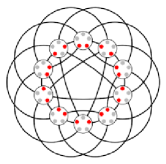
Figure 2: Johnson Graph $J(5,2)$

Proposition 4.1.

Figure 3: Illustration of different cases of the proof of Lemma 4.1

Weetman graphs are simply connected

Proof.

Suppose by contradiction that there is one not contractible cycle $c$ in a Weetman graph $G$. Among all not contractible cycle $c^{\prime}$ in $G$, choose the cycle $c$ minimising $k=d(v_{0},c)=max\{d(v_{0},v^{\prime})\mid v^{\prime}\in c\}$ and minimising $|c\cap S^{k}|$.

We prove that there is another cycles minimising either $d(v_{0},c)$, either $|c\cap S^{k}|$ which is not contractible in $G$, contradicting our hypothesis.

There are two cases, if $|c\cap S^{k}|=1$, then there are $u,v,w\in V(c)$ such that $u,w\in S^{k-1}$, $v\in S^{k}$, $uv,vw\in E(G)$. Moreover, Since $c$ minimises $d(v_{0},c)$, there is no edge $uw\subset E(G)$.

Since $G$ is Weetman, from Condition int applied on the triple of vertices $u,v,w$, there is a path $p=(s_{1}...s_{n})\subset S^{k-1}$ such that $s_{1}=u,s_{n}=w$ and for every $1\leq i\leq n$, $s_{i}v\in E(G)$.

Since the cycle $c^{\prime}=c\setminus\{uvw\}\cup\{p\}$ is related to $c$ by a sequence of elementary homotopies, $c^{\prime}$ is also not contractible and since $d(v_{0},c^{\prime})=k-1$. We get a contradiction on the choice of $c$.

If $|c\cap S^{k}|>1$, let $u\in S^{k-1}$, $v,w\in S^{k}$ such that $u$ and $w$ are the previous and consecutive vertex of $v$ in $c$, i.e. $uv,vw\in E(c)$.

From Condition tri (on the edge $vw$), there is a vertex $z\in S^{k-1}$ such that $zvw\in E(G)$ is a triangle.

From Condition int (on the triple of vertices $uvz$), there is a path $q=\{s_{0}\dots s_{\ell}\}\subset S^{k-1}$ such that $s_{0}=u$, $s_{m}=z$ and $s_{i}v\in E(G),\forall 0\leq i\leq\ell$.

Consequently, there is a cycle $c^{\prime}=c\setminus\{uvw\}\cup\{qw\}$ passing thought vertices $uqw$ instead of $uvw$. Moreover, since $c^{\prime}$ is related to $c$ by a sequence of elementary homotopies, $c^{\prime}$ is also not contractible.

Consequently, since $|c^{\prime}\cap S^{k}|<|c\cap S^{k}|$ and $c^{\prime}$ is not contractible, we get a contradiction on the choice of $c$.

∎

The following Lemma prove that clusters in a simply connected graph have a particular topology that permit us later in this document to explore Weetman Graphs in a quasi optimal way. Since the proof uses combinatorial tools which are not needed in the remaining part, the proof is left to the appendix.

Theorem 1.

Clusters of a simply connected graph form a tree

Consequently, from Theorem 6, we get trivially the next corollary.

Corollary 4.2.

The clusters of a Weetman graph form a tree.

Note that this tree can be reduced to a path in some cases, like Johnson graphs or triangulated sphere. See Fig. 4.

Figure 4: Clusters in a Weetman graph

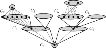
(a) General shape

(b) $Johnson\leavevmode\nobreak\ graph\leavevmode\nobreak\ J(4,2)$

From Corollary 4.2, every cluster $C\subset S^{k}$ of a Weetman graph $G$ admits a unique ancestor cluster, called $a(C)$, in the graph. Note that $a(C)\subset S^{k-1}$ by definition and for the cluster $C_{0}$ containing $v_{0}$, $pred(C_{0})=C_{0}$.

This particularity of Simply connected graph are the basis of the following exploration algorithm. As illustrated in the next corollary, such a property eases the exploration and enables a ”quasi” optimal exploration algorithm.

Corollary 4.3.

Every path leading from the homebase $v_{0}\in V(G)$ of the agent to a connected cluster $C$ goes through $a(C)$.

5 Weetman-universal Exploration Algorithm

Exploring in anonymous graph is difficult. Because of the lack of ids attached to a node, it might not be possible to know whether a node where the agent is located is actually new. We introduce the following terminology. A node is explored if the agent has already been to this node. A node is discovered if it has been seen from another node (that is, if it is adjacent to an explored node). In the following, we give a description of Algorithm 1. In a nutshell, by a DFS traversal of the tree of clusters, for every cluster $C$, the agent will explore all nodes of $C$, discovering in this way all child clusters of $C$. In this way, the agent is able to explore clusters in a DFS fashion.

Algorithm 1 is divided into phases. Between phases, the agent navigates the tree of clusters in a DFS fashion using a stack. In each phase, the agent explores a cluster and updates local structures (more details below). At the end of the phase, the agent extends its map with the new identified vertices and corresponding edges. From the updated map, the agent computes the new clusters that appeared in Map. We now give more details on the computations.

The map Map.

The map computed by the agent is denoted by Map. A vertex $v\in V(G)$ is represented in $V({\textsc{Map}})$ by an unique integer $n$ when the agent identify the vertex $v$. The port numbering of map Map is induced by the port numbering $\delta$ of the network $G$.

Local structures for the identification.

Let $p$ be the path followed by the agent from the beginning of the exploration starting at $v_{0}$. Let $u$ be the current location vertex of the agent in $G$ corresponding to $n$ in its map Map and let $n_{0}$ be the vertex corresponding to the homebase of the agent in Map. That is, $\textsc{dest}_{G}(v_{0},\lambda(p))=u$ and $\textsc{dest}_{{\textsc{Map}}}(n_{0},\lambda(p))=n$.

First, remark that the agent exploring the graph knows in its map on which vertex $n=\textsc{dest}_{{\textsc{Map}}}(n_{0},\lambda(p))$ it is located.

During the exploration of a cluster $C$, for every explored vertex $u\in V(G)$ identified by $n\in V({\textsc{Map}})$. the agent looks through its binoculars, that is, it calls ${\texttt{getBino}}()$ and access to $B_{G}(u,1)$, the ball of radius $1$ around $u$ (Line 1).

The ball $B_{G}(u,1)$ obtained is stored into the set ${\mathcal{B}}$ in order to, at the end of the phase, update and verify the ”local” correctness of the map Map. We denote by ${\mathcal{B}}[n]$ the ball obtained after calling ${\texttt{getBino}}()$ on a vertex $n\in V({\textsc{Map}})$. Since the agent have to know which vertex in ${\mathcal{B}}[n]$ corresponds to its current location, we introduce $\psi(n)\in{\mathcal{B}}[n]$ to denote the vertex corresponding to $n$ in ${\mathcal{B}}[n]$.

At the end of the phase, i.e., the end of the exploration of the cluster, the agent, using ${\mathcal{B}}$, updates two data structures that are used to identify the nodes and update Map.

The first structure PRE-VERT encodes the existence of new vertices that are not present in Map as seen by the agent from an explored node $n$ at the phase $i$.

Since such new vertices are linked to a vertex explored phase $i$, we encode a vertical edge by a tuple $(n,p,q)$ where $n$ is the id of the explored vertex and $(p,q)$ is the labelling of the vertical edge. We call pre-vertex a pair $(n,p)$. Pre-vertices give us all newly discovered vertices. Note that $q$ is stored along the pre-vertex $(n,p)$ only to simplify the computation of Map at the end of the phase.

The main idea to correctly map newly discovered vertices is, at the end of a phase, to find all vertical edges pointing to this node. So, we add a second structure, denoted by ${\mathcal{R}_{\equiv}}$, encoding the elementary relation between two pre vertices corresponding to a same vertex in $G$. So if there is $((n,p),(m,q))\in{\mathcal{R}_{\equiv}}$, then there is a couple of pre-vertices $(n,p),(m,q)\in\texttt{PRE-VERT}$ such that $n$ and $m$ are the ids of vertices explored during the phase, $nm$ is an edge of $E({\textsc{Map}})$ and there is $uvw\subseteq{\mathcal{B}}[n]$ such that $u=\psi(n)$, $\lambda(nm)=\lambda(uv)$ and $\textsc{dest}_{{\textsc{Map}}}(n,\delta_{u}(w))$ is not defined in Map.

In order to update Map in such a way that all edges between discovered nodes are correctly mapped, we have to distinguish two kind of edges. There are edges between an explored node and a newly discovered node. They are called “vertical” edges. But edges between two discovered nodes are also to be correctly mapped. These edges are called “horizontal” edges.

To gather ”vertical” edges, $\equiv$ is sufficient as explained below. To gather ”horizontal” edges, the set Hor is introduced. Since it is not possible to identify ”horizontal” edges before the end of the exploration of the cluster, we store in Hor, together with the port numbers associated to the horizontal edge, only the pre-vertices. Namely, elements of Hor are tuples $(n,p_{1},p_{2},(r,s))$ such that there is a triangle $uvw$ in ${\mathcal{B}}[n]$ where $u=\psi(n)$ and there is two pre vertices $(n,p_{1}),(n,p_{2})\in\texttt{PRE-VERT}$ such that $\delta_{u}(v)=p_{1}$, $\delta_{u}(w)=p_{2}$ and $\lambda(vw)=(r,s)$. Note that by definition, $\textsc{dest}_{{\textsc{Map}}}(n,p_{1})$ and $\textsc{dest}_{{\textsc{Map}}}(n,p_{2})$ are not defined in Map during the exploration of the cluster.

Updating the map.

First remark that the transitive and reflexive closure of $\equiv$, denoted by ${\equiv^{*}}$, is an equivalence relation between pre vertices (it is straightforward that $\equiv$ is reflexive). We denote by $[n,p]$, the representative (or the equivalence class) of a class of pre-vertices including $(n,p)$ via ${\equiv^{*}}$.

To identify new nodes ( Line 1), we compute the quotient of the relation ${\equiv^{*}}$ over pre-vertices stored in PRE-VERT. Then, for every equivalence classes $[n,p]$ of pre-vertices that arises, we add a new vertex $\overline{[(n,p)]}$ in Map. Moreover, every node $n\in V({\textsc{Map}})$ is endowed with an additional label ${\texttt{Cluster}}(n)\in{\mathbb{N}}$ to store the identity of the cluster including $n$.

Then, for every pre vertex $(n,p,q)\in\texttt{PRE-VERT}$, we add a ”vertical” edge linking $n$ to $\overline{[(n,p)]}$ labelled by $(p,q)$ if the edge is not already present in Map.

To update the ”horizontal” edges of Map, for every $(n,p_{1},p_{2},(r,s))\in{\texttt{Hor}}$, we add an edge between $\overline{[(n,p_{1})]}$ and $\overline{[(n,p_{2})]}$ labelled by $(r,s)$ if the edge is not already present in Map.

Additionally, if the agent ends phase $i$, for every vertex $n\in V({\textsc{Map}})$ explored during this phase, ${\texttt{Vis}}(n)$ is set to $i$.

Once Map has been updated, we compare the map obtained and what we saw during the exploration of the cluster. That is, for every vertex $u$ corresponding to $n$ explored phase $i$, we compare $B_{{\textsc{Map}}}(n,1)$ and ${\mathcal{B}}[n]$, the binoculars labelling obtained from $u$. If we detect an error in the map, we decide to continue the exploration forever in order to respect the exploration specification. This case will be more discussed later in this document. If no error is detected, the new clusters that appear in Map are computed, numbered, and push to the stack Stack at Line 1.

The agent stops its exploration when it remains no cluster to explore, that is, when Stack is empty.

Remark 5.1.

The only cluster at level $0$ is composed of the homebase of the agent $v_{0}$.

1 Main Procedure 

2      

3      Add ${\texttt{n}}_{0}$ to $V({\textsc{Map}})$

       ${\textsc{Stack}}\leftarrow{\texttt{Cluster}}({\texttt{n}}_{0})\leftarrow{\texttt{Vis}}({\texttt{n}}_{0})\leftarrow 0$

        /* homebase cluster */

4      

5       while ${\textsc{Stack}}\neq\emptyset$ do

            

              /* Beginning of the phase $i$ */

6             ${\texttt{n}_{\texttt{C}}}\leftarrow$ top element of Stack

7             ${\texttt{C}}\leftarrow\{{\texttt{n}}\in V({\textsc{Map}})\mid{\texttt{Cluster}}({\texttt{n}})={\texttt{n}_{\texttt{C}}}\}$

8             Compute a shortest path Path which from the current location m of the agent, explores the cluster C

             forall the ${\texttt{n}}\in{\texttt{C}}$

              /* Cluster exploration */

9             do

10                   Go to the vertex n following Path

11                   ${\texttt{Vis}}({\texttt{n}})=i$

                   ${\mathcal{B}}[n]\overset{\cup}{\leftarrow}{\texttt{getBino}}({\texttt{n}})$

                    /* Looking thought Binoculars */

12                  

13                  

14             forall the ${\texttt{n}}\in{\texttt{C}}$ do

15                   Get ${\mathcal{B}}[{\texttt{n}}]$ from ${\mathcal{B}}$ and let $u\in V({\mathcal{B}}[{\texttt{n}}])$ corresponding to n

                  

                    /* new pre vertices */

16                   forall the $uw\in E({\mathcal{B}}[{\texttt{n}}])$ s.t. there is no adjacent edge to n in Map labelled by $\lambda(uw)=(\delta_{u}(w),\delta_{w}(u))$ do

17                         $\texttt{PRE-VERT}\overset{\cup}{\leftarrow}({\texttt{n}},\delta_{u}(w),\delta_{w}(u))$

18                        

19                   forall the triangle $uvw\subseteq{\mathcal{B}}[{\texttt{n}}]$ do

                        

                          /* new pre vertices/ vertical relation */

20                         if there is an edge labelled $\lambda(uv)$ and there is no edge labelled $\lambda(uw)$ and $\lambda(vw)$ adjacent to n in Map then

21                               Let $m$ be the vertex in ${\textsc{Map}}^{i}$ such that $nm\in E({\textsc{Map}})$ and $\lambda(nm)=\lambda(uv)$

22                               $\equiv\overset{\cup}{\leftarrow}$ $\Big{(}\big{(}{\texttt{n}},\delta_{u}(w),\delta_{w}(u)\big{)},\big{(}{\texttt{m}},\delta_{v}(w),\delta_{w}(v)\big{)}\Big{)}$

23                              

24                        

                        

                          /* new horizontal edge relation */

25                         if there is no edge labelled by $\lambda(uv),\lambda(uw)$ adjacent to n in Map then

26                               ${\texttt{Hor}}\overset{\cup}{\leftarrow}\big{(}{\texttt{n}},\delta_{u}(v),\delta_{u}(w),(\delta_{v}(w),\delta_{w}(v))\big{)}$

27                              

28                        

29                  

            

              /* Updating Map */

30             forall the $[{\texttt{n}},{\texttt{p}},{\texttt{q}}]\in{\nicefrac{{\texttt{PRE-VERT}}}{{{\equiv^{*}}}}}$ do

31                   Add a new vertex $\overline{[({\texttt{n}},{\texttt{p}})]}$ to Map

32                   ${\texttt{Vis}}(\overline{[({\texttt{n}},{\texttt{p}})]})=\perp$

33                  

34             forall the $({\texttt{n}},{\texttt{p}},{\texttt{q}})\in\texttt{PRE-VERT}$ do

35                   Add a new edge ${\texttt{n}}\overline{[({\texttt{n}},{\texttt{p}})]}$ labelled $({\texttt{p}},{\texttt{q}})$ to Map

36                  

37             forall the $\big{(}{\texttt{n}},{\texttt{p}},{\texttt{q}},({\texttt{p}}^{\prime},{\texttt{q}}^{\prime})\big{)}\in{\texttt{Hor}}$ do

38                   Add a new edge $\overline{[({\texttt{n}},{\texttt{p}})]}\overline{[({\texttt{n}},{\texttt{q}})]}$ labelled $({\texttt{p}}^{\prime},{\texttt{q}}^{\prime})$ in Map

39             if $\forall{\texttt{n}}\in{\texttt{C}}$, ${\mathcal{B}}[{\texttt{n}}]$ is isomorphic to $B_{{\textsc{Map}}}({\texttt{n}},1)$ then

40                   Push in Stack the new clusters in Map

41                   For every new vertex $\overline{[({\texttt{n}},{\texttt{p}})]}$, update ${\texttt{Cluster}}(\overline{[({\texttt{n}},{\texttt{p}})]})$

42            else

43                   Continue forever the execution along an edge

            

              /* End of the phase $i$ */

44            

45      

Algorithm 1 Weetman Graphs Exploration

Let ${\partial{\textsc{Map}}}=\{n\in V({\textsc{Map}})\mid{\texttt{Vis}}(n)=\perp\}$ be the subgraph induced from $G$ composed by the set of vertices in $G$ discovered and not yet explored by the agent.

Note that at ${\textsc{Map}}^{i}$ corresponds to the map computed at the end of the phase $i$.

First we prove the correctness properties, that is, if no error is detected and if the algorithm halts then the graph is explored. Then, the proof of the termination of Algorithm 1 on Weetman graphs will be straightforward.

The core of correctness proof is the following theorem

Theorem 2.

For every phase $i$ of the algorithm, there is an homomorphism $\varphi:M^{i}\to G$ such that

• for every $n\in V({\textsc{Map}}^{i})$, $\varphi_{|N_{M^{i}}(n)}$ is injective

• for every $n\in V({\textsc{Map}}^{i}\setminus{\partial{\textsc{Map}}}^{i})$, $\varphi_{|N_{M^{i}}(n)}$ is surjective

Theorem 2 is proved by an induction on the phases perform by the agent during the execution.

The homomorphism $\varphi$ is based on the following corollary of Theorem 2,

Corollary 5.2.

For every phase $i$, For every vertex $n\in V({\textsc{Map}}^{i})$, for every path $p$ from $n_{0}$ to $n$ in ${\textsc{Map}}^{i}$, $\varphi^{i}(n)=\textsc{dest}_{G}(\varphi(n_{0}),\lambda(p))$

Proof.

Straightforward from Theorem 2 ∎

To ease the notation, an homomorphism $\varphi:{\textsc{Map}}^{i}\to G$ is denoted by $\varphi^{i}$.

Proof of theorem 2

We prove in the next Lemma the initial case of the induction.

Lemma 5.3 (Initial Case).

For any execution of Algorithm 1 on a graph $G$ endowed with a binoculars labelling, ${\textsc{Map}}^{1}$ is isomorphic to $B_{G}(v_{0},1)$.

Proof.

Since for every vertex $v\neq v_{0}$, $d(v_{0},v)>0$, during the first phase, the agent have to explore the first cluster composed by only one vertex, the homebase $v_{0}$. Since the agent is initially located on $v_{0}$, the agent only maps the neighbourhood of the homebase $v_{0}$ during this phase.

Initially, a first vertex ${\texttt{n}}_{0}$ is inserted at Line 1 into ${\textsc{Map}}^{0}$. This vertex identifies the home base $v_{0}$. Let $\varphi({\texttt{n}}_{0})=v_{0}$. At Line 1, $B_{G}(v_{0},1)$ is gathered into ${\mathcal{B}}[{\texttt{n}}_{0}]$. Then, the agent updates its map (Line 1).

• First, since $G$ has an injective port numbering, there is a unique pre-vertex $({\texttt{n}}_{0},{\texttt{p}},{\texttt{q}})$ inserted into PRE-VERT, for every edge $v_{0}w$ in $E(B_{G}(v_{0},1))$ labelled $({\texttt{p}},{\texttt{q}})$.

• Remark that there is exactly one pre-vertex per equivalence classes of pre-vertices. Thus, we get that ${\nicefrac{{\texttt{PRE-VERT}}}{{{\equiv^{*}}}}}\simeq\texttt{PRE-VERT}$.

• Consequently, since one vertex is added into ${\textsc{Map}}^{1}$ for each equivalence class, there is a bijection between $V({\textsc{Map}}^{1})$ and $V(B_{G}(v_{0},1))$.

• Moreover, since there is also one vertical edge inserted at Line 1 for each equivalence class, there is a bijection between vertical edges in $V({\textsc{Map}}^{1})$ and vertical edges in $V(B_{G}(v_{0},1))$.

• It remains to prove that there is also a bijection between horizontal edge of $E({\textsc{Map}}^{1})$ and horizontal edge of $E(B_{G}(v_{0},1))$.

• For every ”horizontal” edge $ww^{\prime}\in E(B_{G}(v_{0},1))$ i.e., $w^{\prime}\neq v_{0}\neq w$, there are $n_{0}\overline{[(n_{0},\delta_{v_{0}}(w))]},n_{0}\overline{[(n_{0},\delta_{v_{0}}(w^{\prime}))]}\in E({\textsc{Map}})$ from the previous case. Moreover, the couple $\Big{(}n_{0},\delta_{v_{0}}(w),\delta_{v_{0}}(w^{\prime}),\big{(}\delta_{w}(w^{\prime}),\delta_{w^{\prime}}(w)\big{)}\Big{)}$ is inserted into Hor at Line 1.

• Thus, an edge $\overline{[(n_{0},\delta_{v_{0}}(w))]}\overline{[(n_{0},\delta_{v_{0}}(w^{\prime}))]}$ labelled by $(\delta_{w}(w^{\prime}),\delta_{w^{\prime}}(w))$ is inserted into $E({\textsc{Map}})$ at Line 1 if and only if there is an edge $ww^{\prime}$ in $G$ labelled by $(\delta_{w}(w^{\prime}),\delta_{w^{\prime}}(w))$.

∎

Consequently, let us define the homomorphism $\varphi^{1}:{\textsc{Map}}^{1}\to G$ such that $\varphi^{1}(n)=\textsc{dest}_{G}(v_{0},\delta_{n_{0}}(n))$, for every $n\in V({\textsc{Map}}^{1})$. Since $\varphi^{1}$ is an isomorphism (Lemma 5.3), we get that at phase $1$, Theorem 2 is proved. Moreover, we get the following Corollary,

Corollary 5.4.

At phase $1$, for every vertex $n\in V({\textsc{Map}}^{1})$, for every path $p$ from $n_{0}$ to $n$ in ${\textsc{Map}}^{1}$, $\varphi^{1}(n)=\textsc{dest}_{G}(\varphi(n_{0}),\lambda(p))$

Phase i-1: (Induction hypothesis)

Suppose that the agent ends phase $i-1>0$ and the agent has computed ${\textsc{Map}}^{i-1}$ such that no error is detected. Moreover, suppose that there is an homomorphism $\varphi^{i-1}:{\textsc{Map}}^{i-1}\to G$ define as follows:

• If $m\in V({\textsc{Map}}^{i-2})$, $\varphi^{i-1}(m)=\varphi^{i-2}(m)$

• If $m\in V({\textsc{Map}}^{i-1}\setminus{\textsc{Map}}^{i-2})$,

  • Let $(n,p)\in\texttt{PRE-VERT}$ such that $\overline{[(n,p)]}=m\in V({\textsc{Map}}^{i-1})$.

  • Let $\varphi^{i-1}(m)=\textsc{dest}_{G}(\varphi^{i-1}(n),\delta_{n}(m))$

Note that by induction and since ${\textsc{Map}}^{i-2}\subseteq{\textsc{Map}}^{i-1}\subseteq{\textsc{Map}}^{i}$, for every $n\in V({\textsc{Map}}^{i-2})$, $\varphi^{i-1}(n)$ is well defined in ${\textsc{Map}}^{i}$. The following corollary explains that the image in $G$ of a vertex in ${\textsc{Map}}^{i-1}$ via $\varphi^{i-1}$ is independent of the path followed by the agent.

Corollary 5.5.

At phase $i-1$, for every vertex $n\in V({\textsc{Map}}^{i-1})$, there is a vertex $w\in V(G)$ such that for every path $p$ from $n_{0}$ to $n$ in ${\textsc{Map}}^{i-1}$, $\varphi^{i-1}(n)=\textsc{dest}_{G}(\varphi^{i-1}(n_{0}),\lambda(p))$

We suppose that Theorem 2 is proved at phase $i-1$, that is, $\varphi^{i-1}$ is locally injective from ${\textsc{Map}}^{i-1}$ and locally surjective from ${\textsc{Map}}^{i-1}\setminus{\partial{\textsc{Map}}}^{i-1}$.

Remark that for every vertex $n\in{\textsc{Map}}^{i-1}\setminus{\partial{\textsc{Map}}}^{i-1}$ ($n$ already explored at phase $i-1$), $B_{{\textsc{Map}}^{i-1}}(n,1)\simeq B_{G}(\varphi^{i-1}(n),1)\simeq{\texttt{getBino}}(n)$.

Phase i:

We prove that when the agent ends phase $i>1$ and has computed ${\textsc{Map}}^{i}$, there is an homomorphism $\varphi^{i}:M^{i}\to G$ such that

• for every $n\in V({\textsc{Map}}^{i})$, $\varphi^{i}_{|N_{M^{i}}(v)}$ is injective

• for every $n\in V({\textsc{Map}}^{i}\setminus{\partial{\textsc{Map}}}^{i})$, $\varphi^{i}_{|N_{M^{i}}(v)}$ is surjective

Next Lemma prove that the relation $\equiv$ gathers in a same equivalence class the maximum set of ”vertical” edges linking a same vertex in $G$. Moreover, it ensure that the image of a vertex via $\varphi^{i}$ as defined above is independent of the choice of the representative $[n,p]$.

Remark 5.6.

Note that in some graphs which are not Weetman, some vertices can be duplicated in Map.

Lemma 5.7.

For every phase $i$ of Algorithm 1, for every pre-vertices $(n,p),(m,q)\in\texttt{PRE-VERT}^{i}$, if $(n,p){\equiv^{*}}(m,q)$ then there is a vertex $w\in B_{G}(\varphi^{i-1}(n),1)\cap B_{G}(\varphi^{i-1}(m),1)$ such that $\varphi^{i-1}(n)w,\varphi^{i-1}(m)w\in E(G)$ and $\delta_{\varphi^{i-1}(n)}(w)=p$ and $\delta_{\varphi^{i-1}(m)}(w)=q$.

Proof.

Suppose that there are two pre-vertices $(n,p),(m,q)\in\texttt{PRE-VERT}^{i}$ such that $(n,p)\equiv(m,q)$.

• From the algorithm, $n$ and $m$ are visited during phase $i$ .

• Moreover, there is a vertex $\overline{[(n,p)]}=\ell\in V({\textsc{Map}}^{i})$ linked to $n$ and $m$ such that $\delta_{n}(\ell)=p$ and $\delta_{m}(\ell)=q$.

• By induction, there is $u,v\in V(G)$ such that $u=\varphi^{i-1}(n)$, $v=\varphi^{i-1}(m)$, and $\varphi^{i-1}(nm)=\varphi^{i-1}(n)\varphi^{i-1}(m)$ is an edge in $E(G)$.

• Moreover, let $p_{n}:n_{0}\to n$ (resp $p_{n}:n_{0}\to m$) denotes the path follows by the agent from the beginning of the execution when it visits $n$ (resp. $m$) for the first time .

• By induction, $\varphi^{i-1}(n)=\textsc{dest}_{G}(v_{0},\lambda(p_{n})))=u$ and $\varphi^{i-1}(m)=\textsc{dest}_{G}(v_{0},\lambda(p_{m})))=v$, that is, $u$ and $v$ are vertices where the agent is located corresponding to $n$ and $m$ in its map.

• Since $(n,p),(m,q)\in\texttt{PRE-VERT}^{i}$ and from from homomorphism definition, the agent has seen two times the triangle $uvw$. Once inside $B_{G}(\varphi^{i-1}(n),1))$ when it visits $n$ such that $\psi(n)=u$ and once inside $B_{G}(\varphi^{i-1}(m),1))$ when it visits $m$ such that $\psi(m)=v$

• Consequently, $w\in B_{G}(\varphi(n),1)\cap B_{G}(\varphi(m),1)$ and there is a vertex $w\in V(G)$ such that $\varphi^{i}(u)w\varphi^{i}(m)$ is a triangle in $E(G)$, we get the first case of this Lemma.

We now prove the case $(n,p){\equiv^{*}}(m,q)$.

• By definition, $(n,p){\equiv^{*}}(m,q)$ implies that there is a sequence of pre vertices $(n_{1},p_{1}),...,(n_{k},p_{k})\in\texttt{PRE-VERT}$ such that

  • $(n,p)=(n_{1},p_{1})$ and $(m,q)=(n_{k},p_{k})$

  • $\forall 1\leq h<k$, $(n_{h},p_{h})\equiv(n_{h+1},p_{h+1})$

• Moreover, by induction, $\varphi^{i-1}(n_{1},...,n_{k})=\varphi^{i-1}(n_{1})...\varphi^{i-1}(n_{k})$ is a path in $G$.

• From the previous case, for every $(n_{h},p_{h})\equiv(n_{h+1},p_{h+1})$, there is $w_{h}\in V(G)$ such that

  • $\varphi^{i-1}(n_{h})\varphi^{i-1}(n_{h+1})w_{h}\subset G$ is a triangle

  • $\delta_{\varphi^{i-1}(n_{h})}(w_{h})=p_{h}$ and $\delta_{\varphi^{i-1}(n_{h+1})}(w_{h})=p_{h+1}$.

• From the transitivity of $\equiv$ and the injective port numbering function of $G$, we get that $\delta_{\varphi^{i-1}(n_{h+1})}(w_{h})=p_{h+1}=\delta_{\varphi^{i-1}(n_{h+1})}(w_{h+1})$.

• Consequently, we get that $w_{h}=w_{h+1}$ for every $1\leq h<k$.

• We prove that there is a unique vertex $w\in V(G)$ such that $\delta_{\varphi^{i-1}(n)}(w)=p$ and $\delta_{\varphi^{i-1}(m)}(w)=q$.

∎

The above Lemma permits us to define the homomorphism $\varphi^{i}:V({\textsc{Map}}^{i})\to V(G)$ such that for every $m\in V({\textsc{Map}}^{i-1})$, $\varphi^{i}(m)=\varphi^{i-1}(m)$ and for every $m\in V({\textsc{Map}}^{i}\setminus{\textsc{Map}}^{i-1})$, $\varphi^{i}(m)=\textsc{dest}_{G}(n,p)$ such that $m=\overline{[(n,p)]}$.

It is straight forward to prove that $\varphi^{i}$ is well defined for vertices. So, we prove in the next lemma that $\varphi^{i}:{\textsc{Map}}^{i}\to G$ is an homomorphism, that is, the image of an edge is an edge.

Lemma 5.8.

At phase $i$, for every edge $nm\in E({\textsc{Map}}^{i})$, $\varphi^{i}(nm)\in E(G)$

Proof.

First, we prove the lemma for vertical edges and then, for horizontal edges.

Vertical edges.

• We know that for every edge $nm\in E({\textsc{Map}}^{i})$ such that $n\notin V({\partial{\textsc{Map}}})^{i}$ and $m\in V({\partial{\textsc{Map}}})^{i}$ (vertical ’edge’), there is a pre-vertex $[n,p]\in\texttt{PRE-VERT}^{i}$ such that $\overline{[(n,p)]}=m$.

• Moreover, there is two vertices $u,v\in V(G)$ such that $\varphi^{i}(m)=v\neq\varphi^{i}(n)=u$ and $\delta_{u}(v)=p$.

• we get that $\varphi^{i}(nm)=\varphi^{i}(n)\varphi^{i}(m)=uv\in E(G)$ is well defined for every ”vertical” edge $nm\in E({\textsc{Map}}^{i})$

Horizontal edges.

Now, we prove that $\varphi^{i}$ correctly maps ”horizontal” edges in Map to $G$.

• By construction, every edge $\overline{[(n,p)]}\overline{[(m,q)]}\in E({\textsc{Map}}^{i}\setminus{\textsc{Map}}^{i-1})$ implies that there is $(n,p,p^{\prime},(r,s))\in{\texttt{Hor}}$ such that $(n,p),(n,p^{\prime})\in\texttt{PRE-VERT}$ are two pre-vertices and $(n,p)\not\equiv(n,p^{\prime})\equiv(m,q)$ (injective port numbering function of $G$) .

• Moreover, the agent located on $u=\varphi^{i-1}(n)$ has seen a triangle $uww^{\prime}\in B_{G}(\varphi^{i-1}(n),1)$ such that

  • the edge $ww^{\prime}$ is labelled $(r,s)$

  • there is no $m,m^{\prime}\in V(B_{{\textsc{Map}}^{i-1}}(n,1))$ such that $\delta_{n}(m)=p$ and $\delta_{n}(m^{\prime})=p^{\prime}$

• From the previous case, $w=\varphi^{i}(\overline{[(n,p)]})$ and $w^{\prime}=\varphi^{i}(\overline{[(m,q)]})$.

• Moreover, since $p\neq p^{\prime}$, $w\neq w^{\prime}$ and thus, $\varphi^{i}(n\overline{[(n,p)]})=vw\neq\varphi^{i}(n\overline{[(n,p^{\prime})]})=vw^{\prime}$.

• Thus, $\varphi^{i}(\overline{[(n,q)]}\overline{[(m,q)]})=\varphi^{i}(\overline{[(n,q)]})\varphi^{i}(\overline{[(m,q)]})=ww^{\prime}\in V(G)$ is well defined for every horizontal edge $\overline{[(n,q)]}\overline{[(m,q)]}$ in $E({\textsc{Map}}^{i})$

∎

By induction, Theorem is already proved for every vertex included in ${\textsc{Map}}^{i-1}$ which are not explored phase $i$. Consequently, we only prove Theorem 2 for

• vertices explored phase $i$ (Lemma 5.9 and 5.10 ), i.e., that belongs to ${\partial{\textsc{Map}}}^{i-1}\setminus{\partial{\textsc{Map}}}^{i}$

• and newly discovered vertices (Lemma 5.11), i.e., that belongs to ${\textsc{Map}}^{i}\setminus{\textsc{Map}}^{i-1}$

Lemma 5.9.

for every $n\in V({\textsc{Map}}^{i}\setminus{\partial{\textsc{Map}}}^{i})$, for every edges $m_{1}m_{1}^{\prime},m_{2}m_{2}^{\prime}\in E(B_{{\textsc{Map}}^{i}}(n,1))$, if $m_{1}m_{1}^{\prime}\neq m_{2}m_{2}^{\prime}$ then $\varphi(m_{1}m_{1}^{\prime})\neq\varphi(m_{2}m_{2}^{\prime})$.

Proof.

Figure 5: Different cases of Lemma 5.9

Let $n\in V({\textsc{Map}}^{i}\setminus{\partial{\textsc{Map}}}^{i})$ be a vertex explored phase $i$ and let $m_{1}m^{\prime}_{1},m_{2}m^{\prime}_{2}\in E(B_{{\textsc{Map}}^{i}}(n,1))$ such that $m_{1}m^{\prime}_{1}\neq m_{2}m^{\prime}_{2}$. Three cases appear,

1. $m_{1}=m_{2}=n$ and $m_{1}^{\prime}\neq m^{\prime}_{2}$.

   • Since $n\in V({\textsc{Map}}^{i}\setminus{\partial{\textsc{Map}}}^{i})$, by induction, ${\mathcal{B}}[n]\simeq B_{G}(\varphi^{i}(n),1)$

   • Since $G$ and ${\textsc{Map}}^{i}$ have injective ports labellings, there is two different vertices $w\neq w^{\prime}\in V(G)$ such that $w=\varphi^{i}(m_{1}^{\prime})\neq w^{\prime}=\varphi^{i}(m_{2}^{\prime})$

   • Thus, since $\varphi^{i}$ is an homomorphism, $\varphi^{i}(w_{1}w_{1}^{\prime})\neq\varphi^{i}(w_{2}w_{2}^{\prime})$

2. $m_{1}=n$ and $m_{1}^{\prime}=m_{2}$

   • First, remark that by definition, for every vertex $m\in V(B_{{\textsc{Map}}^{i}}(n,1))$, there is an edge $nm\in E({\textsc{Map}}^{i})$.

   • So there are $nm_{1}^{\prime},nm_{2}^{\prime}\in E({\textsc{Map}}^{i})$,

   • From the previous case we know that $\varphi^{i}(nm_{1}^{\prime})\neq\varphi^{i}(nm^{\prime}_{2})$.

   • So $\varphi^{i}(m_{1}^{\prime})\neq\varphi^{i}(m_{2}^{\prime})$ and $\varphi^{i}(m_{1}m_{1}^{\prime})\neq\varphi^{i}(m_{2}m_{2}^{\prime})$

3. $n\neq m_{1}\neq m_{2}\neq n$

   • From the previous case $\varphi^{i}(w_{1})\neq\varphi^{i}(w_{2})$ and $\varphi^{i}(w_{1}^{\prime})\neq\varphi^{i}(w_{2}^{\prime})$ in $G$.

   • Since $\varphi^{i}$ is an homomorphism, $\varphi^{i}(w_{1}w_{1}^{\prime})\neq\varphi^{i}(w_{2}w_{2}^{\prime})$

∎

Lemma 5.10.

For every $n\in V({\textsc{Map}}^{i}\setminus{\partial{\textsc{Map}}}^{i})$, $\varphi_{|N_{{\textsc{Map}}^{i}}}(n)$ surjective

Proof.

• Since $\varphi^{i}$ is an homomorphism, every adjacent vertex of $n$ has an image via $\varphi^{i}$.

• Moreover, from Lemma 5.9, $\varphi^{i}$ is locally injective from $B_{{\textsc{Map}}^{i}}(n,1)$ to $B_{G}(\varphi^{i}(n),1)$.

• Consequently, every adjacent vertex of $n$ has a unique image via $\varphi^{i}$.

• Finally, ${\mathcal{B}}[{\texttt{n}}]\simeq B_{{\textsc{Map}}^{i}}(n,1)$ ensures that we map in Map, every vertex present in $B_{G}(\varphi^{i}(n),1)$ which is isomorphic by induction to ${\mathcal{B}}[n]$.

• So, $\varphi^{i}$ is locally surjective for every $n\in V({\textsc{Map}}^{i}\setminus{\partial{\textsc{Map}}}^{i})$ explored phase $i$.

∎

Lemma 5.11.

for every $n\in V({\partial{\textsc{Map}}}^{i})$, $\varphi_{|N_{\textsc{Map}}^{i}}(n)$ injective

Proof.

For every phase $i$, for every $n\in{\partial{\textsc{Map}}}^{i}$, two case appears:

If $n\in V({\partial{\textsc{Map}}}^{i-1})$, then $n$ is not explored phase $i$ and by induction, Lemma is proved.

If $n$ is inserted into Map at phase $i$, that is, $n\in V({\partial{\textsc{Map}}}^{i}\setminus{\partial{\textsc{Map}}}^{i-1})$, then for every neighbours $m\neq m^{\prime}$ of $n$ in $V({\textsc{Map}}^{i})$, two cases appear:

• Either, $m$ and $m^{\prime}$ in $V({\textsc{Map}}^{i}\setminus{\partial{\textsc{Map}}}^{i})$, and in this case, $\Big{(}(m,\delta_{m}(n)),(m^{\prime},\delta_{m^{\prime}}(n))\Big{)}\in{\equiv^{*}}$ . By induction, $\varphi^{i}(m)\neq\varphi^{i}(m^{\prime})$.

• Either, $m$ and $m^{\prime}$ belong to ${\partial{\textsc{Map}}}^{i}$.

  • In such a case, since there is always a vertex $\ell$ (resp. $\ell^{\prime}$) such that $(\ell,\delta_{\ell}(n),\delta_{\ell}(m),\lambda(nm))\in{\texttt{Hor}}$ (resp. $(\ell^{\prime},\delta_{\ell^{\prime}}(n),\delta_{\ell^{\prime}}(m^{\prime}),\lambda(nm^{\prime}))\in{\texttt{Hor}}$)

  • we get that $[\ell,\delta_{\ell}(m)]\neq[\ell,\delta_{\ell}(n)]=[\ell^{\prime},\delta_{\ell^{\prime}}(n)]\neq[\ell^{\prime},\delta_{\ell^{\prime}}(m^{\prime})]$.

  • From previous case, $\varphi^{i}(\ell)\neq\varphi^{i}(\ell^{\prime})$.

  • Since ${\textsc{Map}}^{i}$ has an injective port labelling, $\delta_{n}(m)\neq\delta_{n}(m^{\prime})$.

  • So $\varphi^{i}(m)\neq\varphi^{i}(m^{\prime})$ since otherwise, W.l.o.g. $\delta_{n}(m)\neq\delta_{\varphi(n)}(\varphi(m))$.

∎

We proved the Theorem 2.

It remains to prove that $\varphi^{i}$ preserves triangles in order to prove the correctness of the map construction.

Lemma 5.12.

for every vertex $n\in V({\textsc{Map}}^{i})$ explored phase $i$, for every triangle $v_{1}v_{2}v_{3}\subseteq B_{G}(\varphi^{i}(n),1)$, there is a triangle $m_{1}m_{2}m_{3}\subseteq B_{{\textsc{Map}}^{i}}(n,1)$ such that $\varphi(m_{h})=v_{h}$ for every $1\leq h\leq 3$ and $\varphi(m_{1}m_{2}m_{3})=v_{1}v_{2}v_{3}$

Proof.

for every $n\in V({\partial{\textsc{Map}}}^{i-1}\setminus{\partial{\textsc{Map}}}^{i})$ and for every triangle $v_{1}v_{2}v_{3}\subseteq B_{G}(\varphi^{i}(n),1)$,

• From Lemma 5.9, there is $m_{1}m_{2}m_{3}\in V(B_{{\textsc{Map}}^{i}}(n,1))$ that $\varphi^{i}(m_{1})\neq\varphi^{i}(m_{2})\neq\varphi^{i}(m_{3})$ and $\varphi(m_{1})\varphi(m_{2})\neq\varphi(m_{2})\varphi(m_{3})\neq\varphi(m_{3})\varphi(m_{1})$

• Since we ensure at line 1 that $B_{{\textsc{Map}}^{i}}(n,1)\simeq B_{G}(\varphi(n),1)$, we get that $m_{1}m_{2}m_{3}$ is a triangle in Map if and only if $\varphi^{i}(m_{1})\varphi^{i}(m_{2})\varphi^{i}(m_{3})$ is a triangle in $G$.

∎

Thus, from Lemma above and from Theorem 2, we get the next corollary,

Corollary 5.13.

If, at the phase $i$, the agent halts its exploration (without error), then ${\textsc{Map}}^{i}$ is a simplicial covering of $G$

So we finish this proof by the following Theorem,

Theorem 3.

If the agent halts its exploration, then the graph is explored

Proof.

• First, if the agent halts its exploration then it does not find any mistake in its map (Line 1).

• Moreover, it explores all vertices in its map.

• Suppose the agent halts phase $i$. we get that ${\partial{\textsc{Map}}}^{i}=\emptyset$ (all vertices explored) and thus, ${\textsc{Map}}^{i}$ is locally bijective (injective + surjective).

• $\varphi$ is a covering

• (surjective covering) $|{\textsc{Map}}^{i}|>|G|$

• $G$ is explored

∎

This Theorem means that the agent cannot halts before exploring every vertex of any graph. To conclude this part, we have to prove that the agent always halts on Weetman graphs.

Theorem 4.

For every graph $G\in Weetman$, the algorithm explores $G$ and halts

Proof.

First, note that if the agent halts its execution on a Weetman graph $G$, from Lemma 4.1 and Lemma 5.13, Map is isomorphic to $G$. Moreover, since $G$ satisfied the Interval Condition, every vertex $v$ of $V(G)$ has a unique image $n$ in $V({\textsc{Map}})$. Since $G$ satisfied the Triangle Condition, every edge $\varphi(n)\varphi(m)$ in $E(G)$ has a a unique corresponding image $nm$ in $V({\textsc{Map}})$. Consequently, no error can be found in any execution of ${\mathcal{A}}$ on a Weetman graph $G$ Finally, since the clusters of $G$ form a tree and since the agent performs a DFS over clusters, the agent will reach a phase where all of the nodes in its map are explored. ∎

Remark 5.14.

Let $u,v,w$ be a triple of vertices in $G$ and let $n=\varphi^{i-1}(u),m=\varphi^{i-1}(v)$ and $l=\varphi^{i-1}(w)$ be one pre image of $u,v,w$ in Map and $d(v_{0},w)>d(v_{0},u)=d(v_{0},v)$. If $u,v,w$ does not respect the Interval condition from $v_{0}$ in $G$, then the ”top” vertex $w$ will be duplicated in Map. In fact, since there is no sequence of adjacent triangles $v_{1}v_{2}w,...,v_{k}v_{k+1}w$ in $G$ explored in the same phase, the agent has no enough pre-vertices relation ($\equiv$) at the end of phase to gather $(n,\delta_{u}(w)),(m,\delta_{u}(w))$ in a same equivalence class. Figure 6 illustrates such an error in Map.

Remark 5.15.

So, for every phase $i$, if two vertices in Map are linked to a same vertex in ${\partial{\textsc{Map}}}^{i}$, then we know that there corresponding vertex in $G$ are also linked together with a third vertex which is newly discovered. From the previous remark, we know that we can duplicate a vertex $w$ of $G$ in Map. But in this case, every vertical edge linking $w$ in $G$ are partitioned and distributed over every ”copies” of $w$ in Map (not duplicated).

Figure 6: $IC(v_{0})$ not satisfied on $u,v,w$

5.1 Complexity

Let $G$ be a Weetman graph and let $v$ be the homebase of the agent. Remark that the total number of clusters $|{\mathcal{CIR}}(G)|$ is bounded by $|V|$, $\sum_{C\in{\mathcal{CIR}}_{G}(v)}|V(C)|=|V(G)|$ .

Note that since in a tree $T$, $E(T)=V(T)-1$, exploring a tree takes at most $2|E(C)|\leq 2|V(C)|$ steps even if the agent has to come back to the roots. Moreover, exploring a spanning tree in a graph is a worst case since a cycle in the course of the agent implies that at least one backtracking of the agent is avoided (in front of the spanning tree exploration), which decreases the number of moves.

Since every edge in a cluster is a horizontal edge, the agent crosses at most $\sum_{C\in{\mathcal{CIR}}(G)}2|V(C)|\leq 2|V|$ horizontal edges to explore every cluster.

Horizontal edges in $C$ can be cross two times more. Once the agent goes to the vertex in $C$ which permits it to reach the next cluster $C^{\prime}$ to visit. Once when the agent has finished the exploration of the ”branch” starting at $C^{\prime}$ and backtracks to $C$ to go to the next cluster $C^{\prime\prime}$ to visit. Note that clusters have to be ordered in a way that the agent can go from one to another in a $\mathcal{O}(|V(G)|)$ moves, that is, in a linear number of moves. Moreover, a DFS ordering ensures that once a ”branch” is explored, the agent never returns in this branch. Consequently, we prove that every horizontal edges is crossed by the agent a linear number of times in an execution.

Since ${{\texttt{Cluster}}}(G)$ is a tree and the agent performs a DFS on the clusters, the agent crosses at most two vertical edges per clusters. We get that the agent crosses a linear number of times vertical edges to go from one to another cluster in an execution.

Since the agent explores a spanning tree of $G$, we get that the number of edges crossed is bounded by the number of vertices explores.

Consequently, since we prove that every edge crossed by the agent a linear number of times, the complexity of Algorithm 1 is achieved in $\mathcal{O}(|V(G)|)$ moves.

We get our final theorem,

Theorem 5.

Algorithm 1 explores and computes a map of Weetman graphs with a number of moves that is linear in the size of the graph.

6 Conclusion

We have presented an algorithm that explores all chordal graphs in a linear number of moves by a mobile agent using binoculars to see the edges between nodes adjacent to its location. The main contribution is that the exploration is fast and, contrary to previous works, the agent does not need to know the size or the diameter (or bounds) to halt the exploration. Using binoculars permits to not visit every edge while still being assured of having seen all nodes, which is usually not possible at all without binoculars without additional information about some graph parameters.

We have actually used properties of chordal graphs that are verified in a larger class of graphs : the Weetman graphs. This class of graphs belongs to families of graphs that are defined by local metric properties and whose clique complexes are simply connected, which is a necessary condition for linear exploration without knowledge (see [CGN15]).

Known such families are the family of bridged graphs, or the family of dismantlable/cop-win graphs that have found numerous application in distributed computing. Chordal and bridged graphs are Weetman and Algorithm 1 also efficiently explores these graphs. Dismantlable graphs are not necessarily Weetman, but given that cop-win graphs can also be defined by an elimination order, a very interesting open question would be to prove, or disprove, that there is a linear Exploration algorithm for cop-win graphs.

Appendix 0.A Appendix Section

From the homotopy relation on cycles, we get the following Proposition.

Proposition 0.A.1.

Given a not contractible cycle $c$ in a graph $G$ and a cycle $c^{\prime}$ that is homotopic to $c$, then $c^{\prime}$ is not contractible.

Theorem 6.

Clusters of a simply connected graph form a tree

Proof.

By contradiction, there is two vertices $x,y\in V(G)$ such that $x,y\in S^{k}$ and there is no path $p^{\prime}\subset S^{k}$ from $x$ to $y$. Moreover, to get a cycle of clusters, there is a path $q\subset G\setminus B^{k-1}$ from $y$ to $x$. Note that, W.l.o.g, there is also a path $p:x\to y\subset V(G)$ such that $p\setminus\{xy\}\subset B^{k-1}$.

We denote by $C(x,y)$ a pair of paths $p:x\to y$ and $q:y\to x$ such that $p\setminus\{xy\}\subset B^{k-1}$, $q\subset B^{k+1}$ and ${\mathcal{A}}(C(x,y))$ is minimal.

Among every pair of vertices $x^{\prime},y^{\prime}$ not relied by a path $p^{\prime}\subset S^{k}$, let $x,y$ be the couple minimising ${\mathcal{A}}(C(x,y))$.

Let $a\in p\cap S^{k-1}$ be the vertex such that $ax\in E(p)$ and let $b\in q$ such that $bx\in E(q)$. Remark that since $d(v_{0},x)=k$, we get that $k\leq d(v_{0},b)\leq k+1$

Since $G$ is simply connected, there is a minimal disk diagram $(D,f)$ for the cycle $C(x,y)=pq$. By definition, $f(\partial D)=C(x,y)$ and we denote by ${\widetilde{x}}$ the pre images of $x$ in $D$. W.l.o.g, $f({\widetilde{x}})=x\in V(G)$.

Since $D$ is a planar triangulation, there is a path ${\widetilde{s}}={\widetilde{v}}_{1}{\widetilde{v}}_{2}...{\widetilde{v}}_{\ell-1}{\widetilde{v}}_{\ell}\subset V(D)$ such that for every $1\leq i<\ell$, $f({\widetilde{v}}_{1})=a,f({\widetilde{v}}_{\ell})=b$ and ${\widetilde{x}}{\widetilde{v}}_{i}{\widetilde{v}}_{i+1}$ is a triangle in $D$.

Since $d(v_{0},a)=d(v_{0},x)-1=k-1$ and $k\leq d(v_{0},b)\leq k+1$, for every $1\leq i\leq\ell$, $k-1\leq d(v_{0},v_{i})\leq k+1$.

Consequently, among every ${\widetilde{v}}_{j}\in{\widetilde{s}}$, there is a unique vertex ${\widetilde{v}}_{i}\in{\widetilde{s}}$ such that $d(v_{0},v_{i})=k$ and for every $1\leq h<i$, $d(v_{0},v_{h})=k-1$.

Remark that there is a couple of paths $p^{\prime}:v_{i}\to y$ and $q^{\prime}:y\to v_{i}$ such that $p^{\prime}=p\setminus\{ax\}\cup\{av_{2}...v_{i}\}$, $q^{\prime}=q\cup\{xv_{i}\}$. Moreover, since $x$ and $y$ are not relied by a path in $S^{k}$ and since $v_{i}x\in E(S^{k})$, $v_{i}$ and $y$ are also not relied by a path in $S^{k}$.

Since $p^{\prime}\setminus\{v_{i}y\}\subset B^{k-1}$, and $q^{\prime}\subset G\setminus B^{k-1}$, it remains to prove that ${\mathcal{A}}(p^{\prime}q^{\prime})$ is smaller than ${\mathcal{A}}(pq)$.

Since $D^{\prime}=D\setminus\{uv_{h},\forall 1\leq h<i\}$ is a disk diagram for $p^{\prime}q^{\prime}$, it is easy to see that ${\mathcal{A}}(D^{\prime})<{\mathcal{A}}(D)$ since for every $1\leq h<i$, the triangle ${\widetilde{u}}{\widetilde{v}}_{h}{\widetilde{v}}_{h+1}$ does not appear in $D^{\prime}$.

We get a contradiciton on the choice of $x,y$. Consequently, there is no couple of vertices inside $S^{k}$, for every $k$, which are not relied by a path inside $S^{k}$. We prove that there is no cycle of clusters in simply connected graph and thus, clusters form a tree.

∎

References

- [AGP+11] C. Ambühl, L. Gąsieniec, A. Pelc, T. Radzik, and X. Zhang. Tree exploration with logarithmic memory. ACM Trans. Algorithms, 7(2):17:1–17:21, Mar 2011.
- [AKL+79] R. Aleliunas, R. M. Karp, R.J. Lipton, L. Lovász, and C. Rackoff. Random walks, universal traversal sequences, and the complexity of maze problems. In FOCS, pages 218–223, 1979.
- [BH99] M. Bridson and A. Haefliger. Metric Spaces of Non-positive Curvature. Springer-Verlag Berlin Heidelberg, 1999.
- [BV01] P. Boldi and S. Vigna. An effective characterization of computability in anonymous networks. In DISC, 2001.
- [CFI+05] R. Cohen, P. Fraigniaud, D. Ilcinkas, A. Korman, and D. Peleg. Label-guided graph exploration by a finite automaton. In ICALP, volume 3580 of LNCS, page 335–346, 2005.
- [CGM12] J. Chalopin, E. Godard, and Y. Métivier. Election in partially anonymous networks with arbitrary knowledge in message passing systems. Distrib. Comput., 2012.
- [CGN15] Jérémie Chalopin, Emmanuel Godard, and Antoine Naudin. Anonymous graph exploration with binoculars. In Yoram Moses, editor, Distributed Computing, volume 9363 of Lecture Notes in Computer Science, pages 107–122. Springer Berlin Heidelberg, 2015.
- [Das13] Shantanu Das. Mobile agents in distributed computing: Network exploration. Bulletin of EATCS, 1(109), Aug 2013.
- [GR08] Leszek Gąsieniec and Tomasz Radzik. Memory efficient anonymous graph exploration. In WG, volume 5344 of LNCS, page 14–29, 2008.
- [Ilc08] David Ilcinkas. Setting port numbers for fast graph exploration. Theoretical Computer Science, 401(1–3):236–242, 2008.
- [Kou02] Michal Koucký. Universal traversal sequences with backtracking. Journal of Computer and System Sciences, 65(4):717–726, 2002.
- [LO99] Danny B. Lange and Mitsuru Oshima. Seven good reasons for mobile agents. Commun. ACM, 42(3):88–89, Mar 1999.
- [LS77] R.C. Lyndon and P.E. Schupp. Combinatorial group theory. Ergebnisse der Mathematik und ihrer Grenzgebiete. Springer-Verlag, 1977.
- [Rei08] O. Reingold. Undirected connectivity in log-space. J. ACM, 55(4), 2008.
- [Ros00] Kenneth H. Rosen. Handbook of Discrete and Combinatorial Mathematics. Chapman & Hall/CRC, 2000.
- [RT87] M.A. Ronan and J. Tits. Building buildings. Mathematische Annalen, 278(1-4):291–306, 1987.
- [Wee94] Graham M. Weetman. A construction of locally homogeneous graphs. Journal of the London Mathematical Society, 50(1):68–86, 1994.
- [YK96] M. Yamashita and T. Kameda. Computing on anonymous networks: Part i - characterizing the solvable cases. IEEE TPDS, 7(1):69–89, 1996.