Hi-GAL, the Herschel infrared Galactic Plane Survey: photometric maps and compact source catalogues.

Abstract

Aims. We present the first public release of high-quality data products (DR1) from Hi-GAL, the Herschel infrared Galactic Plane Survey. Hi-GAL is the keystone of a suite of continuum Galactic Plane surveys from the near-IR to the radio, and covers five wavebands at 70, 160, 250, 350 and 500$\mu$m, encompassing the peak of the spectral energy distribution of cold dust for 8$\lesssim T\lesssim$50K. This first Hi-GAL data release covers the inner Milky Way in the longitude range 68^∘$\gtrsim\ell\gtrsim-70$^∘ in a $|b|\leq 1$^∘ latitude strip.

Methods. Photometric maps have been produced with the ROMAGAL pipeline, that optimally capitalizes on the excellent sensitivity and stability of the bolometer arrays of the Herschel PACS and SPIRE photometric cameras, to deliver images of exquisite quality and dynamical range, absolutely calibrated with Planck and IRAS, and recovering extended emission at all wavelengths and all spatial scales, from the point-spread function to the size of an entire 2^∘$\times$ 2^∘ ”tile” that is the unit observing block of the survey. The compact source catalogues have been generated with the CuTEx algorithm, specifically developed to optimize source detection and extraction in the extreme conditions of intense and spatially varying background that are found in the Galactic Plane in the thermal infrared.

Results. Hi-GAL DR1 images are cirrus-noise-limited, reaching the 1$\sigma$-rms predicted by the Herschel Time Estimators for parallel-mode observations at 60^′′ s^-1 scanning speed only in relatively low cirrus emission regions. Hi-GAL DR1 images will be accessible via a dedicated web-based image cutout service. The DR1 Compact Source Catalogues are delivered as single-band photometric lists containing, in addition to source position, peak and integrated flux and source sizes, a variety of parameters useful to assess the quality and reliability of the extracted sources; caveats and hints to help this assessment are provided. Flux completeness limits in all bands are determined from extensive synthetic source experiments and greatly depend on the specific line of sight along the Galactic Plane, due to the greatly varying background as a function of Galactic longitude. Hi-GAL DR1 catalogues contain 123210, 308509, 280685, 160972 and 85460 compact sources in the five bands, respectively.

1 Introduction

The Milky Way Galaxy, our home, is a complex ecosystem in which a cyclical transformation process brings diffuse baryonic matter into dense, unstable condensations to form stars. The stars produce radiant energy for billions of years before releasing chemically enriched material back into the Interstellar medium (ISM) in their final stages of evolution.

Although considerable progress has been made in the last two decades in understanding the evolution of isolated dense molecular clumps toward the onset of gravitational collapse and the formation of stars and planetary systems, a lot remains hidden. We do not know the relative importance of gravity, turbulence or the perturbation from spiral arms in assembling the diffuse and mostly atomic Galactic ISM into dense, molecular, filamentary structures and compact clumps. We do not know how turbulence, gravity and magnetic fields interact on different spatial scales to bring a diffuse cloud to the verge of star formation. We still do not have a comprehensive quantitative understanding of the relative importance of external triggers in the process, although available evidence suggests that triggering is not a major pathway for star formation (Thompson et al., 2012; Kendrew et al., 2012). We do not know how the relative roles played by these different agents changes from extreme environments like the Galactic Centre to the quiet neighbourhoods of the Galaxy beyond the solar circle.

Today, for the first time, it is possible to engage with this ambitious challenge, thanks to a new suite of cutting-edge Milky Way surveys that provide homogenous coverage of the entire Galactic Plane and that have already started to transform the view of our Galaxy as a global star-formation engine (see Molinari et al. 2014 for a recent review).

The UKIDSS Galactic Plane Survey (Lucas et al., 2008) on the 4m UK Infrared Telescope on Hawaii covered the three near-IR photometric bands (J, H and K) to 18^th magnitude, producing catalogues of over a billion stars. The unprecedented depth (15^th mag) and resolution (2^′′) of the NASA Spitzer satellite’s GLIMPSE survey was the first to deliver a new global view of the Galaxy at wavelengths of 3.6, 4.5 5.8, and 8.0$\mu$m (Benjamin et al., 2005), until then only partially accessible from the ground and with imaging capabilities limited to resolutions of a few arcminutes, at best. The resulting catalogue of 49 million sources is dominated by stars and, to a lesser extent, by pre-Main Sequence young stellar objects (YSOs), with the 8.0-$\mu$m channel also showing strong extended emission that probes the interaction between the UV radiation from hot stars and molecular clouds. The Spitzer-MIPSGAL survey at 24$\mu$m (Carey et al., 2009) enables much deeper penetration into the dense molecular clouds to reveal the presence of nascent intermediate and high-mass stars. Such surveys, that were limited to the inner third of the Milky Way Galactic Plane (GP), were complemented by GLIMPSE360, that used Spitzer in its ”warm mission” to complete the coverage of the entire GP at 3.6 and 4.5$\mu$m, and by the WISE satellite (Wright et al., 2010) that, as part of its all-sky survey, is covering the entire GP (although at lower resolution than Spitzer) between 3 and 25$\mu$m.

At far-infrared and millimetre wavelengths, AKARI surveyed the entire sky between 65$\mu$m and 160$\mu$m in 2006–2007. Its spatial resolution of between 1^′ and 1^′​.5 (Doi et al., 2015) represented an improvement of a factor $\sim$3 over that of IRAS, although still a factor $\sim$5 larger than Herschel. The Planck satellite (Planck Collaboration, 2011a) also surveyed the entire sky at wavelengths between 350$\mu$m  and 1cm, but with a resolution ¿5^′, insufficient to resolve the complexity of the thermal dust emission internal to star-forming clouds.

Only ground-based facilities can, at the moment, achieve resolutions below 1^′ in the millimetre regime The ATLASGAL survey (Schuller et al., 2009) has used the 12-m APEX telescope in Chile to map the portion of the GP at longitudes between roughly +60^∘ and $-60$^∘ at 870$\mu$m, the JPS survey (Moore & et al., 2015), using the JCMT antenna in Hawaii, gives deeper coverage at somewhat higher resolution in the northern part of this same region at 850$\mu$m, while the Bolocam GPS covers the 1^st quadrant at 1.1mm (Aguirre et al., 2011). These (sub-)millimetre surveys provide a census of the cold and compact dust condensations that harbour star-formation; however, mass estimates require assumptions about dust temperatures that the single-band survey data themselves cannot constrain.

Radio-wavelength continuum observations provide extinction-free views of bremsstrahlung radiation from ultra-compact HII (UCHII) regions and the ionised ISM in general. The 1^′′​.5 resolution, 6-cm CORNISH survey used the Very Large Array telescope to map the $\ell=+10$^∘ to $+65$^∘ section of the GP at resolutions of $\sim$1^′′ to $\sim$10^′′(Purcell et al., 2013). The CORNISH-South extension of the project, carried out with the ATCA array will complement this information for the corresponding region of the 4^th quadrant, augmented with imaging in radio recombination lines.

This suite of continuum GP surveys sees its ideal complement in a family of spectroscopic surveys of molecular and atomic emission lines. Kinematic information on the same dense clouds traced by the thermal emission from cool dust can also be traced using molecular-line emission. The Galactic Ring Survey (GRS; Jackson et al. 2006), at 46^′′ resolution, uses the FCRAO 14-m antenna to map the ¹³CO (J=1–0) transition in the range 15^∘$\lesssim\ell\lesssim$56^∘. The JCMT COHRS survey (Dempsey et al., 2013) covers essentially the same longitude range as the GRS, but in the CO (J=3–2) line and at a spatial resolution of 14^′′.

Further extensions to the GRS, in the 1^st and 2^nd quadrants, toward the Galactic Anticentre, also in ¹²CO (J=1–0), have been carried out with the FCRAO (Heyer et al., 1998; Brunt & Mottram, 2015). The International Galactic Plane Survey (IGPS) has combined three interferometric 21-cm HI surveys at 45–60^′′ resolution, the combination giving an ideal tool to study the transformation of atomic into molecular gas in the spiral arms (e.g., McClure-Griffiths et al. 2001).

The coverage of the 3^rd and 4^th quadrants in molecular lines is more sparse and less systematic. Together with targeted-source line surveys like MALT90 (Jackson et al., 2013), unbiased coverage of the Plane is limited to the NANTEN survey (e.g. Mizuno & Fukui 2004), now being improved with the NANTEN2/NASCO project that, however, still has limited ($\sim 4$^′) spatial resolution. Recent unbiased surveys with the Mopra antenna in Australia (Burton et al., 2013; Jones et al., 2012) are starting to fill the gap with the data quality of the CO surveys in the northern portion of the GP. The SEDIGISM survey is currently in execution to map the 4^th quadrant between $\ell=+18$^∘ and $\ell=-60$^∘ in ¹³CO and C¹⁸O (J=2–1) with the APEX telescope.

The Methanol Multi-Beam survey (e.g., Green et al. 2012) is searching the Plane for 6.7-GHz methanol maser emission using the Parkes and ATCA telescopes. Methanol maser emission is characteristic of the early formation stage of massive stars; its association with cool dense clumps is a signpost for ongoing formation of massive stars and associated protoclusters in such objects. A more complete compilation of GP Surveys from the near-IR to the radio is provided in the review of Molinari et al. (2014).

The Herschel infrared Galactic Plane Survey (Hi-GAL, Molinari et al. 2010b, a), carried out with the Herschel Space Observatory (Pilbratt et al., 2010), is the keystone in the arch of GP continuum surveys. With a full Plane coverage of the thermal far-IR and submillimetre continuum in five bands between 70$\mu$m and 500$\mu$m, ideally covering the peak of the spectral energy distribution (SED) of dust in the temperature range 8 K$\leq T\leq 50$ K, Hi-GAL delivers a complete census of structures containing cold dust, from the Central Molecular Zone to the outskirts of the Galaxy, enabling self-consistent determination of dust temperatures and masses. Thanks to its space-borne platform, the Herschel cameras do not suffer from the rapid atmospheric variabilities that limit ground-based submillimetre facilities. This allows full exploitation of the excellent sensitivity and stability of the infrared bolometric arrays to deliver exquisite-quality images that recover extended emission from dust on all spatial scales. The ability of Herschel to recover multi-wavelength extended emission from the diffuse ISM, through dense filamentary structures, down to compact and point-like sources (Molinari et al., 2010a; André et al., 2010) are and will remain unparalleled in the coming decades.

Hi-GAL is delivering a transformational view of the complete evolutionary path that brings cold and diffuse interstellar material to condense into clouds and filaments that then fragment into protocluster-forming dense clumps. More than 50 papers have been published by the Hi-GAL consortium to date, based on Hi-GAL images and preliminary source catalogues, from studies of the diffuse ISM (e.g. Bernard et al. 2010; Paradis et al. 2010; Compiégne et al. 2010; Traficante et al. 2014; Elia et al. 2014) to dense, large-scale filaments (Molinari et al., 2010a; Schisano et al., 2014; Wang et al., 2015), dust in HII regions (e.g. Paladini et al. 2012; Tibbs et al. 2012, clumps and massive star formation (e.g. Elia et al. 2010; Bally et al. 2010; Elia et al. 2013; Battersby et al. 2011; Mottram & Brunt 2012; Wilcock et al. 2012; Veneziani et al. 2013; Beltrán et al. 2013; Strafella et al. 2015; Traficante et al. 2015), Galactic Central Molecular Zone studies (Molinari et al., 2011a; Longmore et al., 2012), triggered star formation (Zavagno et al., 2010) and finally dust around post-Main Sequence objects (Umana et al., 2012; Martinavarro-Armengol et al., 2015). More papers are in preparation in the Hi-GAL Consortium. Although basic Hi-GAL data have always been open for public access through the Herschel Science Archive, we are now providing access for the larger Community to the high-quality data products (maps and source catalogs) used internally by the Hi-GAL consortium.

In this paper we present the first public release of Hi-GAL data products (DR1). DR1 is limited to the inner Milky Way in the longitude range +68^∘$\geq\ell\geq-70$^∘ and latitude range 1^∘$\geq b\geq-$1^∘, and consists of calibrated and astrometrically registered images at 70, 160, 250, 350 and 500$\mu$m, plus compact-source catalogues, delivered via an image cutout service provided by the ASI Science Data Center and accessible from the VIALACTEA project portal at http://vialactea.iaps.inaf.it. We present and discuss the production methods and characterization of the images and catalogues considered according to their band-specific properties. A full systematic analysis of the physical properties of dense, star-forming and potentially star-forming condensations (reconstructed from the band-merged Hi-GAL photometric catalogues with augmented SED coverage from ancillary surveys from the mid-IR to the millimetre), will be presented in Elia et al. (2016). A first systematic analysis of far-IR properties of post-Main Sequence objects based on the Hi-GAL Catalogues is presented in Martinavarro-Armengol et al. (2015).

2 Observations

The motivations and observing strategy adopted for the Hi-GAL Survey are described in detail in Molinari et al. (2010b). The complete survey was assembled in three instalments of observing time granted in Open Time competition in each of the three calls issued during the Herschel project lifetime. Due to a clerical inconsistency in determining the duration time of the observations, a longitude range of about 6^∘ in extent in the outer Galaxy could not be executed in the observing time formally granted for the complete Plane coverage, and Director’s Discretionary Time was additionally granted to obtain the 360^∘-wide coverage. The total observing time amounted to slightly in excess of 900 hours, making the full Hi-GAL survey the largest observing program carried out by Herschel.

The Hi-GAL observations were acquired by subdividing the surveyed area into square tiles of $\sim$ 2^∘.2 in size, to obtain complete coverage of a $|b|\leq 1$ strip of the Galactic Plane at 70, 160, 250, 350 and 500$\mu$m simultaneously. Each tile was observed with the PACS (Poglitsch et al., 2010) and SPIRE (Griffin et al., 2010) cameras in parallel mode (pMode), specifically designed to optimise data acquisition for large-area multi-wavelength surveys. In pMode the PACS and SPIRE cameras are used simultaneously, effectively making Herschel into a five-band imaging camera spanning a decade in wavelength. Since the field of view of the PACS and SPIRE cameras are offset by $\sim 20$′ in the plane of the sky, slight oversizing of the individual observing tiles was needed to make sure that a 2^∘x2^∘ area was covered in all five photometric bands.

As the bolometers that constitute the elemental pixels of the PACS and SPIRE arrays are differential detectors known to be affected by slow thermal drifts with typical $1/f$ frequency behaviour, each tile was observed in two independent passes with nearly orthogonal scanning directions. Individual Astronomical Observation Requests (AORs) were concatenated in the Herschel Observation Planning Tool (HSpot) so that the two scanning passes were executed immediately one after the other for each tile. This strategy was chosen so that a given position in the sky was observed by as many pixels as possible and in different scanning directions, producing the degree of redundancy needed to beat down the correlated and uncorrelated $1/f$ noise of single detectors, thereby allowing recovery of all the emission at the largest possible spatial scales. The approach was also designed to perfectly couple to the data processing and map-making pipeline specifically developed for the Hi-GAL project (see §3).

The satellite scan speed in pMode was set to its maximum value of 60 ″ per second, with a detector sampling rate of 40 Hz for PACS and 10 Hz for SPIRE. The spatial sampling is therefore 1.5″ and 6.0″ for PACS and SPIRE, respectively, enough to Nyquist sample all the nominal diffraction-limit beams ($\simeq$[6.0, 12.0, 18.0, 24.0, 35.0]″ at [70,160, 250, 350, 500] $\mu$m, respectively). However, due to the limited transmission bandwidth, the PACS data were co-added on-board Herschel, with a compression of 8 and 4 consecutive frames at 70 and 160 $\mu$m, producing an effective spatial sampling of 12″ and 6″ at 70 and 160 $\mu$m respectively. Therefore, in pMode, the PACS beams are not Nyquist sampled and the resulting point-spread functions (PSFs) are elongated along the scan direction with a measured size of 5.8″$\times$12.1″and 11.4″$\times$13.4″ at 70 $\mu$m and 160 $\mu$m, respectively (Lutz 2012).

Table 2 summarizes a few details of the observations. Column 1 is an assigned field name for each tile; cols. 2-5 report the approximate coordinates of the tile centre; cols. 6 and 7 indicate the date of the observation for each tile, both in standard format and in OD number (Observation Day, starting from date of launch); cols. 8-10 report the start time (UT) of the tile in the nominal and orthogonal scan direction (see below), together with the associated observation identification (OBSID) number uniquely attached to each scan observation.

SPIRE was used in “bright-source” mode in the three tiles of the survey closest to the Galactic Centre (roughly centred at longitudes +2^∘, 0^∘ and $-$2^∘). This was done to avoid the widespread saturation and non-linearities in the detector response otherwise likely to occur on the extraordinarily strong background emission in that region. In this observing mode, the limited 12-bit dynamical range of the Analog-to-Digital converters in the detector chains is centred around higher-than-nominal current values. In this way saturation is avoided at the cost of greatly decreased sensitivity. In “bright-source” mode SPIRE is much less capable of detecting intermediate and low-flux compact sources (see fig. 20, last three panels).

Table 1: The log of the observations.

Field	RA	Declination	$\ell$	b	Date	OD	Nominal		Ortho.
	hh:mm:ss	dd:pp:ss					Start	OBSID	Start
290	11:05:14.266	$-$60:57:38.79	290.400	$-$0.700	2010-08-15	459	15:42:32	1342203081(+1)	18:21:52
292	11:22:31.063	$-$61:42:12.77	292.600	$-$0.629	2010-08-14	458	20:53:20	1342203065($-$1)	18:01:48
294	11:40:34.588	$-$62:18:00.17	294.800	$-$0.552	2010-08-14	458	26:24:29	1342203067($-$1)	23:32:57
297	11:59:16.713	$-$62:44:25.30	297.000	$-$0.471	2010-08-15	458	07:55:37	1342203069($-$1)	05:04:05
299	12:18:26.910	$-$63:00:59.70	299.200	$-$0.384	2009-09-03	112	03:21:32	1342183075(+1)	06:26:26
301	12:37:52.625	$-$63:07:23.91	301.400	$-$0.292	2010-08-15	459	24:06:14	1342203084($-$1)	21:14:42
303	12:57:20.191	$-$63:03:29.76	303.600	$-$0.194	2010-01-08	239	04:03:19	1342189081(+1)	07:15:22
305	13:16:35.719	$-$62:49:20.56	305.800	$-$0.091	2010-01-08	239	13:40:19	1342189084($-$1)	10:27:43
308	13:35:27.781	$-$62:26:15.89	308.000	0.000	2010-08-16	459	05:38:17	1342203086($-$1)	02:46:45
310	13:53:56.541	$-$61:59:11.46	310.200	0.000	2010-08-20	464	22:27:35	1342203279($-$1)	19:36:03
312	14:11:47.708	$-$61:23:08.81	312.400	0.000	2010-01-09	240	04:06:20	1342189110($-$1)	00:53:44
314	14:28:53.915	$-$60:38:41.13	314.600	0.000	2010-08-21	464	01:07:08	1342203280(+1)	03:46:28
316	14:45:10.082	$-$59:46:25.81	316.800	0.000	2010-08-21	464	06:37:45	1342203282(+1)	09:17:05
319	15:00:33.335	$-$58:47:02.32	319.000	0.000	2010-08-21	465	17:57:13	1342203289(+1)	20:36:33
321	15:15:02.740	$-$57:41:10.22	321.200	0.000	2010-08-21	465	26:19:33	1342203292($-$1)	23:28:01
323	15:28:38.841	$-$56:29:28.17	323.400	0.000	2010-01-29	261	24:48:03	1342189879($-$1)	21:35:27
325	15:41:23.367	$-$55:12:32.49	325.600	0.000	2010-08-22	465	04:59:07	1342203293(+1)	07:38:27
327	15:53:18.797	$-$53:50:57.02	327.800	0.000	2010-09-03	478	24:11:19	1342204043($-$1)	21:19:47
330	16:04:28.099	$-$52:25:12.66	330.000	0.000	2010-09-04	478	05:42:27	1342204045($-$1)	02:50:55
332	16:14:54.520	$-$50:55:47.08	332.200	0.000	2010-09-04	478	08:21:47	1342204046(+1)	11:01:07
334	16:24:41.348	$-$49:23:05.26	334.400	0.000	2010-09-04	479	24:20:00	1342204055($-$1)	21:28:28
336	16:33:51.865	$-$47:47:29.17	336.600	0.000	2010-09-05	479	05:51:08	1342204057($-$1)	02:59:36
338	16:42:29.198	$-$46:09:18.44	338.800	0.000	2010-09-05	479	11:22:16	1342204059($-$1)	08:30:44
341	16:50:36.309	$-$44:28:50.42	341.000	0.000	2010-09-06	480	13:55:21	1342204095($-$1)	11:03:49
343	16:58:15.976	$-$42:46:20.19	343.200	0.000	2010-09-06	480	08:24:15	1342204093($-$1)	05:32:43
345	17:05:30.743	$-$41:02:01.36	345.400	0.000	2010-09-06	480	02:53:09	1342204091($-$1)	00:01:37
347	17:12:22.972	$-$39:16:05.62	347.600	0.000	2010-09-06	481	25:27:08	1342204101($-$1)	22:35:36
349	17:18:54.803	$-$37:28:43.53	349.800	0.000	2011-02-20	647	07:34:31	1342214511($-$1)	04:42:59
352	17:25:08.192	$-$35:40:04.45	352.000	0.000	2011-02-20	648	20:02:47	1342214576($-$1)	17:11:15
354	17:31:04.932	$-$33:50:16.46	354.200	0.000	2011-02-24	651	04:29:59	1342214713(+1)	07:09:19
356	17:36:46.638	$-$31:59:27.04	356.400	0.000	2010-09-12	486	12:19:22	1342204369($-$1)	09:27:50
358	17:42:14.801	$-$30:07:42.57	358.600	0.000	2010-09-12	486	06:48:07	1342204367($-$1)	03:56:26
0	17:45:37.199	$-$28:56:10.23	000.000	0.000	2010-09-07	481	04:08:11	1342204102(+1)	06:47:44
2	17:50:46.049	$-$27:03:08.22	002.200	0.000	2010-09-07	481	09:39:03	1342204104($-$1)	12:18:36
4	17:55:44.665	$-$25:09:25.47	004.400	0.000	2011-02-24	652	13:30:00	1342214761(+1)	16:09:20
6	18:00:34.119	$-$23:15:06.43	006.600	0.000	2011-02-24	652	19:01:17	1342214763(+1)	21:40:37
8	18:05:15.396	$-$21:20:15.19	008.800	0.000	2011-04-09	695	02:11:54	1342218963(+1)	04:51:14
11	18:09:49.409	$-$19:24:55.45	011.000	0.000	2011-04-09	695	07:43:15	1342218965(+1)	10:22:35
13	18:14:17.005	$-$17:29:10.63	013.200	0.000	2011-04-10	696	13:36:51	1342218999(+1)	16:16:11
15	18:18:38.972	$-$15:33:03.90	015.400	0.000	2011-04-10	696	10:57:27	1342218998($-$1)	08:05:55
17	18:22:56.053	$-$13:36:38.19	017.600	0.000	2011-04-10	696	05:26:14	1342218996($-$1)	02:34:42
19	18:27:08.946	$-$11:39:56.26	019.800	0.000	2011-04-15	701	09:54:54	1342218644(+1)	12:34:14
22	18:31:18.313	0$-$9:43:00.72	022.000	0.000	2011-04-15	701	07:15:30	1342218643($-$1)	04:23:58
24	18:35:24.790	0$-$7:45:54.02	024.200	0.000	2011-04-15	701	15:26:36	1342218646(+1)	18:05:56
26	18:39:28.986	0$-$5:48:38.52	026.400	0.000	2011-04-16	702	14:23:37	1342218696(+1)	17:02:57
28	18:43:31.490	0$-$3:51:16.53	028.600	0.000	2011-04-16	702	08:52:59	1342218694(+1)	11:32:19
30	18:46:05.222	0$-$2:36:32.90	030.000	0.000	2009-10-24	163	02:33:54	1342186275(+1)	05:39:08
30filler	18:48:28.610	0$-$1:09:31.80	031.563	+0.130	2011-10-24	893	09:38:00	1342231361(+1)	10:40:30
33	18:51:33.726	0+0:03:38.13	033.000	0.000	2011-04-16	702	06:13:19	1342218693($-$1)	03:21:47
35	18:55:34.588	0+2:01:06.44	035.200	0.000	2011-04-26	712	16:39:59	1342219631($-$1)	13:48:27
37	18:59:36.031	0+3:58:32.52	037.400	0.000	2010-10-23	528	24:48:50	1342207027($-$1)	21:57:18
39	19:03:38.623	0+5:55:54.18	039.600	0.000	2010-10-24	528	06:19:59	1342207029($-$1)	03:28:27
41	19:07:42.942	0+7:53:09.18	041.800	0.000	2010-10-24	528	11:51:08	1342207031($-$1)	08:59:36
44	19:11:49.580	0+9:50:15.27	044.000	0.000	2010-10-24	529	26:42:28	1342207053($-$1)	23:50:56
46	19:15:59.148	+11:47:10.05	046.200	0.000	2010-10-25	529	08:13:37	1342207055($-$1)	05:22:05
48	19:20:12.280	+13:43:51.05	048.400	0.000	2011-11-05	905	06:33:30	1342231859($-$1)	03:41:58
50	19:24:29.643	+15:40:15.66	050.600	0.000	2011-11-04	904	08:55:34	1342231851(+1)	11:34:54
52	19:28:32.384	+17:38:53.32	052.800	+0.088	2011-10-23	892	10:22:02	1342231342($-$1)	07:30:30
55	19:32:35.799	+19:37:48.65	055.000	+0.198	2011-05-02	718	13:13:23	1342219813($-$1)	10:21:51
57	19:36:46.510	+21:36:13.38	057.200	+0.301	2011-05-02	718	18:44:29	1342219815($-$1)	15:52:57
59	19:41:44.297	+23:01:21.60	059.000	0.000	2009-10-23	162	10:28:59	1342186235(+1)	13:34:13
59filler	19:44:00.000	+24:10:00.00	060.250	+0.119	2011-11-05	905	09:14:34	1342231860(+1)	10:16:38
61	19:45:33.109	+25:31:19.18	061.600	+0.492	2011-05-03	719	15:17:59	1342220536($-$1)	12:26:27
63	19:50:10.833	+27:27:53.52	063.800	+0.579	2011-10-23	892	04:49:22	1342231340($-$1)	01:57:50
66	19:54:59.545	+29:23:43.65	066.000	+0.661	2011-10-22	892	23:18:16	1342231338($-$1)	20:26:44

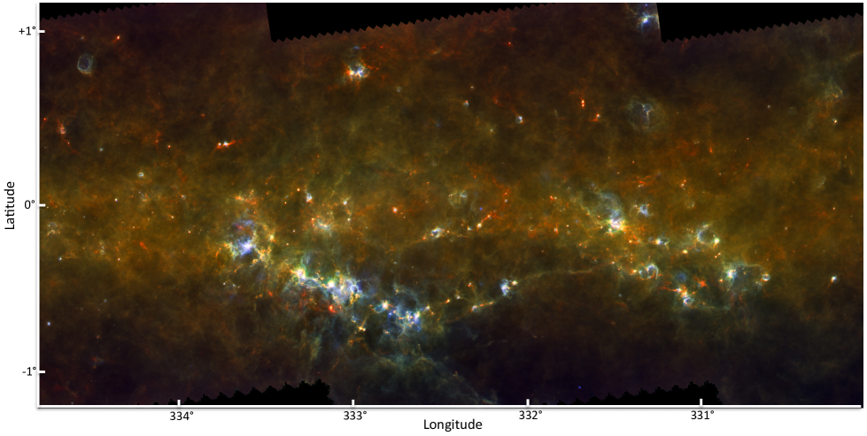
Figure 1: Three-colour image (blue 70$\mu$m, green 160$\mu$m, red 350$\mu$m) of a 3-tile mosaic field around 330^∘$\lesssim\ell\lesssim$335^∘.

3 Production of the Photometric Maps

The data reduction was carried out using the ROMAGAL data-processing software described in detail in Traficante et al. (2011). In short, the pipeline uses standard Herschel Interactive Processing Environment (HIPE) (Ott, 2010) processing up to level 0.5, where the signal from individual detectors is photometrically calibrated and each detector has its sky position assigned. Subsequent steps in the data reduction were carried out using a dedicated pipeline written within the Hi-GAL Consortium. Fast and slow detector glitches arising from particle hits onto the detectors are identified and the affected portions of the data are flagged in each detector’s Time Ordered Data (TOD). Slow detector drifts arising from $1/f$ noise are estimated and subtracted; for PACS, the drifts are estimated at subarray level as each $16\times 16$ array matrix shares the same readout electronics. The core of the map-making implements a Generalised Least-Square (GLS) algorithm that is ideally designed to use redundancy to minimise residual uncorrelated $1/f$ detector noise by filtering in Fourier space (Natoli et al., 2001). In order to deliver optimal results, the code (i.e. each GLS-based code) requires that the detector noise properties are regularly sampled in time over the entire duration of the observations. For this reason we implement a pre-processing stage where the sections of the TOD flagged as ”bad data” (e.g. due to a glitch removal or signal saturation) are replaced with artificial samples in which the data are set to 0, but where the noise is added using a ”constrained noise realisation” using the noise frequency properties estimated from valid data immediately before and after the flagged section.

The pixel sizes of the ROMAGAL maps account for the larger-than-nominal PACS PSFs and are set to [3.2, 4.5, 6.0, 8.0, 11.5]″ at [70, 160, 250, 350, 500] $\mu$m respectively. This choice represents a good compromise between the need to sample the PSF as also determined for point-like objects in Hi-GAL maps with at least three pixels, while avoiding (in the case of PACS 70$\mu$m and 160$\mu$m) excessively small pixels in which the hit statistics of the detector sampling are too low, resulting in increased pixel-to-pixel noise. For the PACS bands this is due to the fact that the Herschel scanning strategy in pMode implements an on-board frame co-adding (see §2), resulting in an effective decrease in sampling rate. The pixel size of the images is therefore such that the beam FWHM is sampled with 3 pixels for the three SPIRE bands, and with 2.66 pixels in the PACS bands. Saturated pixels in the maps are a consequence of signal saturation for all TODs covering the specific pixel, due to the necessary limitations in the dynamical range of DAC converters at the detection stage. A list of locations where saturation is reached is reported in appendix B.

It is clearly not possible to report in the paper, even in electronic form, the complete list of images for all wavelengths and all the tiles of Table 2. We choose here to show only one figure (Fig. 1) as a 3-colour image of a 3-tile mosaic in the longitude range 330^∘$\lesssim\ell\lesssim$335^∘to set the framework for the subsequent sections (see §4 and §5.1) describing the properties of the compact-source catalogues. The maps deliver a stunning view of the GP at all Hi-GAL wavelengths with a detail that is unattainable from any ground-based millimetre-wave facility now and in the foreseeable future. Extended emission with at least two orders of magnitude dynamical range in intensity is retrieved at all spatial scales from the most compact objects to the extent of the entire tile. We will show in the next sections that compact sources within these multiple complex, extended structures have very low peak/background contrast ratio (generally below 1). This makes the detection and flux computation of compact sources an extremely complex task, where it is, in particular, difficult to identify a figure of merit that can be used to unambiguously distinguish reliable from unreliable sources.

The pipeline is augmented with a module specifically developed by the Hi-GAL team to cure the high-frequency artefacts that the GLS map-making technique used in ROMAGAL (as in many other approaches, like MadMap or Scanamorphos) is known to introduce to the maps, namely crosses and stripes corresponding to the brightest sources. The left panel in Fig. 2 shows a typical example of these features that are introduced by the noise filter deconvolution carried out by the GLS map-maker in Fourier space when the flux is strongly varying with position, as is the case for point-like sources. We find that the minimum within a negative cross feature is proportional to the peak brightness of the source, and amounts to $\sim 2.5$% of this value. It is therefore not a strong effect in principle, but is can be quite annoying for relatively faint nearby objects and for the determination of the surrounding diffuse emission; it is also aesthetically undesirable.

To correct for such effects, particularly visible in the PACS 70-$\mu$m, and to a lesser extent, in the 160-$\mu$m images, a weighted post-processing of the GLS maps (WGLS, Piazzo et al. 2012) has been applied to finally obtain images in which these artefacts are removed (right panel in Fig. 2).

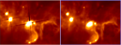
Figure 2: Left panel: Particulars of a point source as reconstructed by the ROMAGAL map-making for PACS at 70$\mu$m; the typical ”cross” feature introduced by the GLS map-maker when performing the noise filter deconvolution in Fourier space over strongly varying signal (as is the case for point-like sources) is clearly seen (image in log scale). The minimum within the negative cross scales as $\sim 2.5$% of the peak source flux. Right panel: same as left panel with the same scale and colour stretch, but after applying the correction devised by Piazzo et al. (2012). The angular extent of the region imaged is $\sim$6^′$\times$ 4^′.

3.1 Noise properties of the Hi-GAL maps

To characterize the noise properties of the Hi-GAL DR1 maps, we consider all the tiles in each band, locating and analyzing those map regions where the lowest signal is found. This is done by computing the pixel brightness distribution and selecting pixels where the brightness is below the lowest 10% percentiles. We subsequently consider, always for each tile and each band separately, only those pixels that form connected areas with at least 100 pixels each and we therein compute the median of the brightness and the mean of its r.m.s. These quantities are reported in Fig. 3 as full and dashed lines, respectively, as function of Galactic longitude. The figure reports for each band the distribution of the lowest brightness levels, and the corresponding r.m.s., found in each tile. The coloured ticks on the right margin of the figure represent the 1$\sigma$ brightness sensitivities in MJy/sr predicted by the PACS and SPIRE time estimator for the Hi-GAL observing strategy, with two independent orthogonal scans taken in parallel mode at a scanning speed of 60^′′ s^-1 .

Brightness levels are always well above the instrument sensitivities, showing that, even in the faintest regions mapped by Hi-GAL, we are limited by cirrus brightness and cirrus noise emission by big grains (Desert et al., 1990) for $\lambda\geq$ 160$\mu$m, except perhaps at the outskirts of the Hi-GAL DR1 longitude range where the minimum signal r.m.s. is close or equal to the predicted detector noise. An exception is the 70-$\mu$m emission, where the brightness of the diffuse cirrus that dominates at longer wavelengths drops significantly (Bernard et al., 2010). The 70-$\mu$m brightness levels reach (or cross) the respective r.m.s. values much earlier, moving away from the Galactic Centre, than in the other bands. The fact that the most intense emission is reached at 160$\mu$m, and then decreases toward 500$\mu$m is in excellent agreement with expectations for diffuse, optically thin cirrus dust at temperatures 16 K $\lesssim T\lesssim$20 K, as determined by Paradis et al. (2010) from detailed modelling of Hi-GAL data in selected regions of the Galactic Plane.

It should be noted that the Hi-GAL ROMAGAL pipeline used for DR1 is successfully delivering the PACS and SPIRE predicted sensitivities with the very bright and complex ISM emission on the Galactic Plane, while preserving in the data processing chain the signal at all spatial scales with no spatial scale filtering.

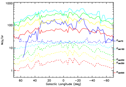
Figure 3: Distribution as a function of Galactic longitude of the median brightness (full lines) and its r.m.s. (dashed lines), in regions within each Hi-GAL tile where the brightness levels are below the 10% percentiles of the brightness distribution for that tile. Hi-GAL bands are colour-coded as: blue for PACS 70$\mu$m, cyan for PACS 160$\mu$m, green for SPIRE 250$\mu$m, yellow for SPIRE 350$\mu$m and red for SPIRE 500$\mu$m. Ticks on the right margin of the figure mark the values of the theoretical sensitivities predicted by the official PACS/SPIRE time estimator (available in HSpot) for observations in pMode with 60^′′ s^-1 scanning speed.

3.2 Astrometric corrections

Although the map-making algorithm was run for each tile using the same projection centre for all bands, the PACS and SPIRE maps are slightly mis-aligned, possibly due to a residual uncalibrated effect in the basic astrometric calibration that is carried out in the HIPE environment. Excellent map alignment is essential to generate products such as column-density maps (e.g. Elia et al. 2013) or to positionally match source counterparts at different wavelengths.

As the images obtained with the same instrument (PACS or SPIRE) are internally aligned, we initially align the PACS 70$\mu$m images to match the astrometry of the Spitzer/MIPSGAL images at 24$\mu$m. This has the advantage that the two instrument/wavelength combinations deliver the same spatial resolution. The astrometric accuracy of the MIPSGAL images with respect to higher resolution IRAC and 2MASS is better than $\sim$1″ on average (Carey et al., 2009).

Figure 4: Top Panel:Astrometry shifts in Galactic longitude ($x$ axis) and latitude ($y$ axis), estimated for each tile in arcseconds. Crosses are for PACS tiles while triangles are for SPIRE tiles. The error bars represent the r.m.s. of the source coordinates used to estimate the offset corrections with respect to their respective mean value. Bottom Panels: Histograms of the r.m.s. of the longitude (full lines) and latitude (dashed lines) shifts estimated for PACS (left panel) and SPIRE (right panel).

For each tile For each tile, we visually select a number of sources across the maps (typically more than 6) that appear relatively isolated and compact both at 24 and 70$\mu$m. The implicit assumption is that the two counterparts are the same physical source; This is reasonable as long as we avoid selecting sources in relatively crowded star forming regions where sources in different evolutionary stages (and hence intrinsically different SED shapes) are generally found. We extract the selected sources in both images and we determine an average $\overline{[\delta l,\delta b]}$ shift to minimize the offsets between the positions of the selected sources in the 24-$\mu$m and 70-$\mu$m maps. This mean shift correction is then applied to the astrometric keywords in the FITS headers of the PACS maps.

The SPIRE maps were aligned by bootstrapping from the aligned PACS images. For each tile we selected a number of sources that appear compact and isolated both in PACS 160$\mu$m and SPIRE 250$\mu$m. In a similar way to the alignment of the 70-$\mu$m PACS images, we extract the selected sources in both maps and compare the source positions in the two bands to determine an average shift that minimizes the positional differences. This average shift is then applied to correct the astrometric keywords in the FITS headers of all SPIRE maps.

The corrections estimated for each tile are shown in Fig. 4 for PACS (cross signs) and SPIRE (triangles) images, taking the Spitzer/MIPSGAL images as a reference. Corrections can be as large as 6^′′ in absolute terms, meaning they are particularly significant for the PACS 70-$\mu$m band where they can reach about 2/3 of the image reconstructed FWHM beamwidth. The outlier point at the top-right of the plot corresponds to the tile centred at $\ell$=299^∘, which was taken during the Herschel Performance Verification Phase. The Herschel astrometric accuracy evolved throughout the mission, as sources of errors in the star trackers and in general in the pointing reconstruction have been isolated and recovered. One of the major issue up to OD 320 was the “speed bumps” that caused large variations in the scanning speed of the telescope. These bumps happened when a tracking star passed over bad pixels of the optical telecope’s CCD. This effect was corrected by lowering the operational temperature of the tracking telescopes. In general, the astrometric accuracy up to OD 320 was better than 2 arcsec but outliers at more than 8 arcsec were observed (for a detailed report on the Herschel astrometric accuracy see Sánchez-Portal et al. 2014).

The error bars in Fig. 4 represent the r.m.s. of the source coordinates used to estimate the offset corrections with respect to their mean value. The distribution of these values is reported in the lower panels of Fig. 4; they are centred around the median values [$\Delta$GLON, $\Delta$GLAT]=[0^′′​.9, 0^′′​.8] for the PACS images (lower-left panel of fig. 4), and [1^′′​.7, 1^′′​.6] for the SPIRE images (lower-right panel), and may be assumed as an estimate of the typical residual uncertainty of the source coordinates. These amount to $\sim$ 10% of the PSF FWHM as estimated from compact sources in the images. It is interesting to note that there are a few outliers in the distributions, particularly apparent for the PACS shifts, but even for their maximum values they are below half of the PACS beam at 70$\mu$m. As mentioned at the beginning of the section, an additional average 1^′′ uncertainty should be added in quadrature to account for the MIPSGAL pointing accuracy.

3.3 Map photometric offset calibration

Although the PACS and SPIRE images are calibrated internally in Jy/pixel and Jy/beam, respectively, their zero point level is not. So in order to bring the images to a common calibrated zero level an offset was applied to the maps. The photometric offsets of the Hi-GAL maps were determined through a comparison between the Hi-GAL data and the Planck and IRIS (Improved Reprocessing of the IRAS Survey) all-sky maps, following the procedure described in Bernard et al. (2010). We smoothed the Herschel maps to the common resolution of the IRIS and Planck high frequency maps of 5′ and projected them into the HEALPix pixelisation scheme (Górski et al., 2005) following the drizzling procedure described in Paradis et al. (2012), which preserves the photometric accuracy of the input maps. These smoothed Hi-GAL maps are compared with the IRIS and Planck all-sky maps (hereafter called ”model”).

To make this model, we used the IRIS maps projected into HEALPix taken from the CADE web site (http://cade.irap.omp.eu) and the Planck maps shown in Planck Collaboration (2011b). Since the Herschel, Planck and IRAS photometric channels are different, the comparison requires frequency interpolation with differential colour correction, and the use of a model. We predict the shape of the emission spectrum in each pixel using the DustEM code (Compiégne et al., 2011), computed for an intensity of the radiation field best matching the dust temperature, derived from the combination of the IRIS 100-$\mu$m and the Planck 857-GHz and 353-GHz maps. The dust temperature assumed is that of Planck Collaboration (2011b) with the standard dust distribution of Compiégne et al. (2011). For a given PACS or SPIRE band, the model is normalized to the data at the IRAS or Planck band at the nearest frequency to the considered Herschel band, and a predicted 5′ resolution model image is constructed.These nearest frequencies are the IRAS 60-$\mu$m and Planck 857-GHz bands for the PACS 70-$\mu$m and 160-$\mu$m bands, respectively, and the Planck 857-GHz, 857-GHz and 545-GHz bands for the SPIRE 250-$\mu$m  350-$\mu$m and 500-$\mu$m bands, respectively. In this process, the differential colour correction between IRAS or Planck and the Herschel band under consideration is also taken into account, using the spectral shape predicted by the model on a pixel-by-pixel basis.

This resulting model image is compared with the smoothed Hi-GAL data through a linear correlation analysis, the intercept of which provides the offset level to be added to the Herschel data to best match the IRIS and Planck data. This analysis also provides gain corrections (i.e. a slope of unity between the data and the model); however, these are well below the cumulative relative uncertainties in the datasets used, as well as in the dust modelling assumptions, and within 10%, on average, in all bands. The standard Herschel photometric calibration was therefore assumed, and no additional gain corrections were applied. Note also that the Planck data used does not have the same absolute calibration as the publicly available version. A forthcoming processing of the Hi-GAL data will use the latest Planck calibration and will allow for a global gain correction.

4 Generation of Photometric Catalogues from Hi-GAL maps

In comparison to the ground-based submillimetre-continuum surveys, the Herschel instruments do not suffer from the need to correct for varying atmospheric emission and absorption, allowing recovery of the rich and highly structured large-scale emission from Galactic cirrus and extended clouds. Such variable and complex backgrounds, however, severely hinder the use of traditional methods to detect compact sources based on the thresholding of the intensity image. Such methods are widely used by large-scale millimetre and radio surveys from ground-based facilities, like the Bolocam GPS (Rosolowsky et al., 2010), CORNISH (Purcell et al., 2013) or ATLASGAL (Contreras et al., 2013), where diffuse emission is filtered out either by atmospheric variation correction or the instrumental transfer function. The possibility of processing Herschel images using high-pass filtering was discarded for various reasons. First of all, it would be difficult to choose a threshold in spatial scale. Dust cores and clumps are compact but, depending on their distance and physical scale, may not be point-like (i.e., unresolved). A spatial filtering scale threshold too close to the PSF will remove power from compact but resolved sources, while a threshold large enough to make sure that no power is removed from scales corresponding to 2-3 times the PSF will prove ineffective to improve source detection in crowded fields. A second reason is that any high-pass spatial filtering will introduce negative lobes with intensities proportional to the brightness of the extended emission, severely hindering the detection of faint sources that fall within those features.

In a previous work, Molinari et al. (2011b) introduced a new method to detect sources and extract their fluxes tailored to the case of the complex and structured background present in IR/sub-mm observations. With respect to other popular algorithms, the CuTEx photometry code, standing for Curvature Thresholding Extractor, adopts a different design philosophy, looking for the pixels in the map with the highest curvature by computing the second derivative of the map. All the “clumps” of pixels above a defined threshold are analyzed and the ones larger than a certain area are kept as candidate detections. The pixels of the large “clumps” are checked to determine enhancement of curvature in the case of multiple sources. For each detection, an estimate for the size of the source is determined by fitting an ellipse to the positions of the minima of the second derivative in each of the 8 principal directions. The output fluxes and sizes are determined by simultaneously fitting elliptical Gaussian functions plus a 2^nd-order 2D surface for the background. All the sources whose detected centres are closer than twice the instrumental PSF are fitted together to disentangle their fluxes.

The Gaussian fitting is carried out for each source by considering a fitting window centred on each source and with a width of 3 times the instrumental PSF to make sure to include sufficient space surrounding the source for a reliable estimate of the background. This has the drawback that the pixels used to constrain the background are numerically predominant with respect to the pixels characterising the source; to counterbalance this effect, the pixels located within a distance equal to the initial guesstimated source size from the source position are given a higher weight in the fit.

4.1 The characterization of the photometric algorithm

CuTEx, as a derivative-based detection algorithm, acts as a high-pass spatial filter; however, contrary to simple median or boxcar filtering, derivative filtering has inherent multiscale capabilities by selectively filtering out the larger the spatial scales in a continuous way with higher efficiency. Such behaviour is shown in Fig. 5, where we report, for Gaussians with increasing widths, the ratio between the second derivative image and the original one at the peak position, as a function of the spatial scale expressed in pixels. The results shown are obtained on a simulated image where the FWHM of the PSF is sampled by three pixels, and therefore is a general result applicable to any map that shares this characteristic, like the Herschel maps we present here. Fig. 5 shows that the peak intensity of a point-like source, with a FWHM of $\sim$3 pixels (i.e. 1 PSF), is damped in the second derivative image to $\sim$40% of its original value, while an extended source with FWHM of $\sim$ 7.5 pixels (i.e. 2.5 $\times$ PSF) and the same peak intensity is damped to $\sim$10% of the original value. In other words, a point source in the intensity map that is, say, 10 times fainter (contrast 0.1) than the surrounding background, with typical scale of order 15 pixels, i.e. 5 $\times$ PSF, will appear in the derivative map as $\sim$1.7 times brighter than the background (contrast 1.7). Given the trend in Fig. 5, where attenuation declines following a power-law behaviour with an exponent –2, it is then possible to detect sources with less favourable contrast the larger is the background typical scale. Clearly, the method has the inherent drawback of being most effective for more compact objects (see below).

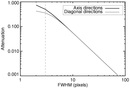
Figure 5: Relative attenuation of the peak intensity induced by the derivative filtering as a function of the scale of the structure. The diagonal directions have been divided by $\sqrt{2}$ to take into account the longer distance along the diagonals with respect to the normal axis. For scales longer than $\sim$ 6 pixels, the damping increases as a power law function with an exponent $-2$. The dark grey dashed line refers to the typical size in pixels of the PSF in Hi-GAL maps.

To confirm the performances of CuTEx’s derivative operator in the case of real maps, we computed the power spectrum of the second derivative image for each map, averaging the spectra obtained for each derivative direction. We then divided each derivative power spectrum by the power spectrum of the parent intensity image. These ratios are proportional to the module square of the transfer function of the derivative operator used by CuTEx. Fig. 6 shows these ratios for 5 different maps (indicated with different colours in the figure) in the case of 250-$\mu$m observations. Similar plots are found for the other wavelengths, where the only difference is a shift in angular spatial scale due to the different pixel scales. The scale in the upper $x$ axis is in pixels and insensitive to the specific pixel angular scale.

Several conclusions can be drawn from the analysis of these functions. First, the transfer function is the same, regardless of the mapped region, for scales larger than the PSF. Second, the damping introduced by the derivative operator found in Fig. 5 is confirmed also for real maps. From an investigation of a sample of very extended sources in the Hi-GAL maps, we estimated that CuTEx is not able to recover most of the sources with sizes larger than 3 times the PSF (see also Fig. 18), being completely insensitive to any source larger than $\sim$5 times the PSF. The third conclusion resulting from Fig. 6 is that the derivative filtering introduces an amplification for scales smaller than the PSF. This means that any pixel-to-pixel noise present in the intensity map is increased in the second derivative maps. Slight differences between the different tested fields are only visible at scales below the PSF (the dashed line in the figure) but are not relevant for the detection of real sources. To quantify such an increase, we tested the effect of the derivative operator on pure Gaussian noise maps and found that the noise in the second derivative follows the same distribution with a standard deviation 1.13 times the initial one. Such behaviour is not unexpected, due to the linearity properties of the derivative filtering.

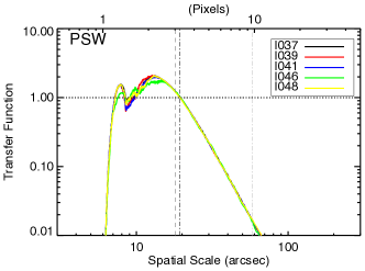
Figure 6: Ratio between the power spectrum of the derivative images (averaged over the four directions) computed by CuTEx, and the power spectra of the intensity image for SPIRE 250$\mu$m, as a function of spatial scale expressed in arcseconds and in pixels (upper $x$ axis). Each colour corresponds to a different map; respectively, black l037, red l039,blue l041, green l046, yellow l048 field. All the functions overlap for scales larger than the PSF, indicated as a dark grey dashed line, and decrease following a power-law with an exponent $\sim$ –3.9. The black dot dashed line indicates the scale at which the transfer function is equal to unity. Scales smaller than that result in an overall amplification in the second derivative maps. The light grey dot-dashed line traces the scale above which the extended sources start to get confused with the background in the derivative image. Such value corresponds approximately to $\sim$ 3 times the PSF. Similar plots are found for other wavelengths and the functions completely overlap when the spatial scales are expressed in pixels.

4.2 Choice of the extraction threshold

In similar way to source extraction performed on images of surface brightness distribution, it is useful to set an extraction threshold as a function of the local curvature r.m.s. instead of adopting a constant absolute value. In this way, the depth of the extraction is adapted to the complexity of the morphological properties and to the intensity of the background that constitutes the dominant flux contribution in the far infrared toward the GP.

Although the adoption of a detection threshold in the second derivative image is certainly less intuitive than adopting a threshold on the flux brightness map, we have shown above that the noise statistical properties do not change when going from flux maps to flux curvature maps (except for a small increase in the width of the noise distribution), so that the notion of a threshold that adapts to the local noise properties can be applied also to detection on the curvature images.

The choice of an optimal source extraction threshold always results from a compromise between the need to extract the faintest real sources, and the need to minimize the number of false detections. Pushing the detection threshold to lower and lower values to extract fainter and fainter sources is of course of minimal use if the majority of such faint extracted sources have a high probability of being false positives, therefore considerably limiting the catalogue completeness and reliability. Unfortunately there is no exact way to control the number of false positives extracted from real images, as there is no control list for real sources present, so that a number of a posteriori checks are needed to determine this optimal threshold value.

The procedure we adopted to estimate the optimal extraction threshold is to make extensive synthetic source experiments to characterise the flux completeness levels obtained for different CuTEx extraction thresholds $\sigma_{c}$ in all five Hi-GAL photometric bands, where $\sigma_{c}$ is in units of the r.m.s. of the local values of the second derivatives of the image brightness averaged over 4 directions (see Molinari et al. 2011b).

As it is clearly impractical to make these studies over the entire set of Hi-GAL tiles, we chose three tiles at Galactic longitudes of 19, 30 and 59 degrees that are representative of the widely variable fore/background conditions that can be found over the entire survey. For each of these tiles and for each observed band, hundreds of synthetic sources were injected at different flux levels. We then ran CuTEx for a set of extraction thresholds $\sigma_{c}$ from 3 to 0.5, estimating for each threshold the flux for which 90% of the synthetic sources were successfully recovered. We verified that, for each of the three tiles, the 90% completeness fluxes decrease with decreasing extraction threshold. In the case of the three SPIRE bands, we see that this decrease flattens, starting at $\sigma_{c}\sim 2$, meaning that we do not gain in depth of extraction by going to lower thresholds. We emphasize that our artificial source experiments provide the same optimal value for the extraction threshold independently of the tile used, in spite of the very different properties of the diffuse and structured background exhibited by the Hi-GAL images in the longitude range covered in DR1. This is a convenient feature of the detection method, that is clearly able to deliver similar performances with very similar parameters in widely different fields. We then adopt $\sigma_{c}=2$ as the extraction threshold for the SPIRE bands.

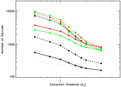
Figure 7: Top Panel: Number of sources extracted with CuTEx as a function of extraction threshold for the 70-$\mu$m (thick solid lines), 160-$\mu$m (thick dashed lines) and 250-$\mu$m bands (dotted thick lines), for three Hi-GAL tiles with very different background conditions: $\ell$=19^∘ (green lines), $\ell$=30^∘ (red lines) and $\ell$=59^∘ (black lines). The thin dotted lines are power-law fits to the initial and mid portions of the N-$\sigma_{c}$ relationship at 70$\mu$m for the $\ell$=59^∘ tile, and are shown to emphasize the change in slope that is visible for all functions for $\sigma_{c}\lesssim 2$. Bottom Panel: Detection statistics for the simulated source experiments reported in Fig. 7 of Molinari et al. (2011b) for a flux of 0.1 Jy; the total number of simulated sources is 1000. The full line reports the number of true sources recovered, while the dashed line reports the number of false positives as a function of extraction threshold. It is noticeable how the number of false positives increases faster for decreasing thresholds than the number of true sources detected, qualitatively explaining the change of slope in the real fields detections (top panel).

In the case of the PACS 70-$\mu$m and 160-$\mu$m bands, the decrease of the 90% completeness fluxes continues below $\sigma_{c}$=2. This apparent gain in the number of reliable sources detected at lower and lower thresholds is likely to be due to increasing numbers of false-positive detections. We characterize the impact of false positives by evaluating the number of extracted sources in the different bands as a function of the extraction threshold. Fig. 7-top reports the number of sources detected in the three tiles (indicated by the different colours) at 70, 160 and 250$\mu$m (solid, dashed and dotted lines) as a function of the extraction threshold. The figure shows that in all cases the N$-\sigma_{c}$ relationships tend to get steeper below $\sigma_{c}\sim 2$; we emphasize this in Fig. 7 in one case by fitting two power-laws to two portions of the N-$\sigma_{c}$ for the 70-$\mu$m case of $\ell$=59^∘ (the two thin dotted lines). A similar behaviour is exhibited for all the other cases, and we interpret this increase of rate in detected sources for $\sigma_{c}\leq 2$ as an indication of increased contamination of false detections. It is, strictly speaking, impossible to verify this claim on real images, because we do not have a truth table for the sources that are effectively present. We then make use of a subset of the extensive simulations that we did in Molinari et al. (2011b) where we presented and characterized the CuTEx package; the bottom panel of Fig. 7 reports the number of true detected sources (full line) and the number of false positives (dashed line) as a function of the extraction threshold for a simulation of 1000 synthetic sources (that were reported in the top-left panel of Fig. 7 in Molinari et al. 2011b). It can indeed be seen that for decreasing extraction thresholds, the number of false-positive detections increases faster than the number of real sources. It is irrelevant here to compare the absolute values of the slopes between the real and simulated cases in Fig. 7, nor the thresholds where the false positives may become dominant, because the two cases refer to very different situations (see Molinari et al. (2011b) for more informations on the simulations carried out). What is important here is that the faster increase of false positives with respect to real sources as a function of decreasing threshold may qualitatively explain the change of slopes in the detection rates with thresholds that we see in the real fields in the top panel of Fig. 7.

In order to be conservative for this first catalogue release, we choose to adopt an extraction threshold of $\sigma_{c}$=2 also for the 70$\mu$m and 160-$\mu$m PACS bands. We believe that the detection threshold could be pushed to lower values especially in the PACS bands and toward low absolute Galactic longitudes; this requires more extensive studies of the completeness level analysis and characterizations of the real impact of false positives contamination and will be deferred to the release of subsequent photometric catalogues.

4.3 Generation of the source catalogues

Sources were extracted independently for each Hi-GAL tile and for each band using CuTEx with extraction threshold $\sigma_{c}=2$. As each map tile results from the combination of two observations of the same area scanned in nearly orthogonal directions, and since the area scanned in the two different directions is never exactly the same, the marginal areas of the combined maps will generally be covered only in one direction, resulting in very poor quality compared to the majority of the map area. For this reason, we exclude such areas from the source extraction. The selection of the optimal map regions is performed manually for each tile and separately for the PACS and SPIRE images. These regions will always be at the margins of the tiles but this does not result in gaps in longitude coverage, since the contiguous border region of any tile will be optimally covered by the adjacent tile.

The full source extraction was carried out on an IBM BladeH cluster with 7 blades, each equipped with Intel Xeon Dual QuadCores, for a total of 56 processors. Each independent tile and band extraction job was dynamically queued to each processor, allowing us to complete the extraction from 63 2^∘$\times$ 2^∘ tiles in five bands in one day. The different photometry lists for each band were then merged together to create complete single-band source catalogues. As there is always a small overlap between adjacent Hi-GAL tiles, some sources may be detected in two tiles. In this case, where source positions match within one half of the instrumental beam, the detection with the higher signal-to-noise (SNR) ratio was accepted into the source catalogue. The number of compact sources extracted over the longitude range considered in this release are reported in Table 2.

Table 2: Source numbers in the Hi-GAL photometric catalogues

Band	Nsources
PACS-70$\mu$m	123,210
PACS-160$\mu$m	308,509
SPIRE-250$\mu$m	280,685
SPIRE-350$\mu$m	160,972
SPIRE-500$\mu$m	85,460

The CuTEx algorithm detects sources by thresholding on the values of the curvature of the image brightness spatial distribution, and as such is optimised to detect compact objects that may be more extended than the instrumental beam. The analysis reported in section 4.1 shows that the 2^nd-order derivative processing ensures differential enhancement of smaller spatial scales with respect to larger scales also above the instrumental PSF. In section 5.3 below, we verify that the majority of extracted sources have sizes that span the range between 1 and 3 times the instrumental PSF, with most of the objects below 2-2.5 times the beam (see Fig. 18) and axis ratio below 2 (see Fig. 19). In the rest of the paper we will refer to the Compact Source Catalogues, to signify that the catalogues include relatively round objects with sizes generally below 2-2.5 times the beam.

The catalogues contain basic information about the detection and the flux estimation for all sources, including source position, peak and integrated fluxes, estimated source size and uncertainty computed as the brightness residuals after subtraction of the fitted source+background model. The calibration accuracy of the PACS photometer is of the order of 5% in all bands (Balog et al., 2014), due to the uncertainties in the theoretical models of the SED of the stars used as calibrators. For SPIRE the main calibrator is Neptune and, as for PACS, the main uncertainty comes from the theoretical model of the planet emission and it is estimated at 4% in all the bands (Bendo et al., 2013).

Hi-GAL photometric catalogues are ASCII files in “IPAC Table” format, and contain information on source position, peak and integrated fluxes, source sizes, locally estimated noise and background levels, and a number of flags to signal specific conditions found during the extraction. The full list of the 60 table columns, with explanation of the column contents, can be found in Appendix A; given the number of columns, it is not possible to show a preview of the catalogue tables in a printed form. The DR1 single-band photometric catalogues are delivered to ESA for release through the Herschel Science Archive, and are available via a dedicated image cutout and catalogue retrieval service accessible from the VIALACTEA project portal http://vialactea.iaps.inaf.it.

4.4 Catalogue Flux Completeness

To quantify the degree of completeness of the extracted source lists we carried out an extensive set of artificial source experiments by injecting simulated sources into real Hi-GAL maps. Given the very time-consuming nature of these experiments, we chose to carry them out for each band but only for a subset of the entire range of longitudes that is the subject of the present release. We visually selected one from every 2-3 tiles, depending on the variation of the emission seen in the maps as a function of Galactic longitude. We used a similar methodology as in §4.2 for the determination of the optimal extraction threshold, but this time we use only one detection threshold and an adaptive grid of trial fluxes for the synthetic sources.

For each band of this subsample, we injected 1000 sources modelled as elliptical Gaussians of constant integrated flux, with sizes and axis ratios equal to the majority of the compact sources determined from the initially extracted list (see Figs. 18 and 19). In this way, we are able to test the ability to recover a statistically comparable population of sources from the same map. The sources are randomly spread on the map, with the only constraint being to avoid overlap with the positions of the real sources.

The simulated data are processed with CuTEx , adopting the same setup of parameters used for the initial list and the outputs are compared with the truth table of the injected sources. To have an estimate on the errors we iterated the experiment 10 times and determined how the fraction of recovered sources varies. The same process is iterated for different values of integrated flux until the fraction of recovered sources is 90% (with a tolerance of 1%). An example of the recovery fraction as a function of the integrated flux density of the injected sources is given in Fig. 8.

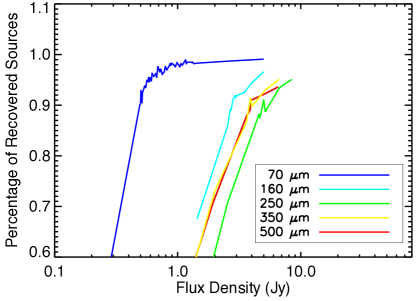
Figure 8: Completeness fractions as a function of flux density for the map centred at $(\ell,b)$ = (19,0), a field with a very intense and complex background at the boundary of the Central Molecular Zone, in the different Herschel bands for sources with statistically the same sizes as those in the extracted catalogue.

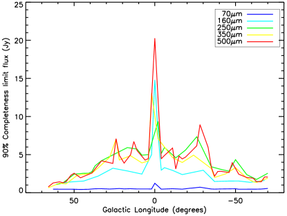
Figure 9: 90% completeness limits in flux density for a population of sources with the same distribution of sizes as the one extracted by CuTEx  as a function of Galactic longitude. The significant increase in the completeness limit in the inner Galaxy and especially close to the Galactic Centre is due to the brighter background emission in such regions.

In Fig. 9, we show the estimated completeness limit as a function of Galactic longitude. The limits for the PACS 70-$\mu$m and 160-$\mu$m bands are quite regular along the whole range of longitude. However, while the completeness in the 70-$\mu$m band is almost constant, at 160$\mu$m it is higher for $\lvert\ell\rvert\leq$ 40. Such a behaviour is more significant in the SPIRE wavebands and increases while moving toward the Galactic Centre. It is explained by the overall brighter emission at lower longitudes, making the detection of fainter objects a harder task, even with the strong damping induced by CuTEx.

The completeness limits reported in Fig. 9 should be seen as conservative because they are determined by spreading the synthetic sources randomly over each entire tile. However the diffuse background is highly non-uniform in each tile, but it is dominated by the strong GP emission with a maximum in the central horizontal section of each map, and then decreasing toward the north and south Galactic directions. A typical example is offered in Fig. 10 where, in the upper panel, we show the 250-$\mu$m image of the tile centred at $\ell$=41^∘. Superimposed are the extracted 250-$\mu$m compact sources with integrated fluxes above (yellow crosses) and below (magenta crosses) the flux completeness limit appropriate for the Galactic longitude at that band (3 Jy, from Fig. 9). This is also shown in the lower panel of Fig. 10, where the latitude distribution of the two groups of sources is also reported with full/dashed lines for sources above/below the confusion limit.

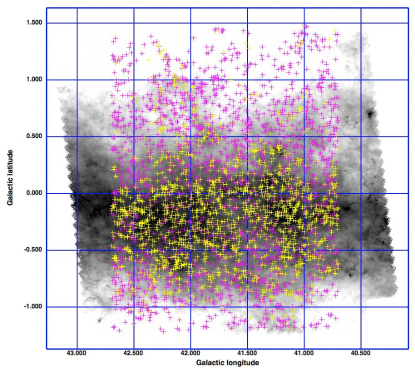
Figure 10: Upper panel: 250-$\mu$m image of the Hi-GAL tile at $\ell$=41^∘ with superimposed the sources detected with CuTEx. The yellow crosses indicate the sources with fluxes above the completeness limit, while the magenta crosses indicate the sources with fluxes below the completeness limit. Lower panel: histograms of latitude distributions for 250-$\mu$m sources, above (full line) and below (dashed line) the completeness limit.

The two groups of sources have a very different spatial distribution, with sources brighter than the completeness limit mostly concentrated at –0^∘​.6 $\leq b\leq$ 0^∘​.2 while the fainter sources are uniformly distributed and mostly found toward the map areas where the diffuse emission is relatively less intense. The dashed line in the lower-panel histogram is flat because fainter sources are better detected in lower surface-brightness regions (above and below the Plane) than in the central band of the Plane.

In subsequent releases of the Hi-GAL photometric catalogues we will provide more precise estimates of the catalogue completeness limits specific to different background conditions.

4.5 Deblending

CuTEx is designed to fit a gaussian function to each position where there is an enhancement of the 2^nd derivative with respect to its nearby environment. While the flux estimate relies on the performance of the fitting engine as well as on the fidelity of the gaussian model fit to the real source profiles, it is clearly important to quantify the ability of the photometric algorithm to separate individual sources in the case where they are very close to each other. To quantify the deblending performance of the algorithm we generated simulations with 2000 sources randomly distributed on a region whose size represents the typical footprint of the Hi-GAL maps. For every set of positions we produced two different sets of simulated populations. In the first case, we injected sources with sizes of the order of the beam size. In the second case we simulated a population of extended sources modeled as elliptical gaussians with the FWHM of one of the two axes drawn from a uniform distribution between 1 and 2.5 times the beam size. The other axis is determined by assuming an axis ratio randomly drawn from a uniform distribution between 0.5 and 1.5 times the beam size. The input sources are randomly oriented. We computed several simulations with different positions and increasing source densities in order to estimate the deblending performance for cases of both lesser and greater clustering.

Figure 11: The curves represent the fraction of blended sources that CuTEx is not able to deblend as a function of source separation for a set of synthetic sources described in the text; simulations in this case are made for the 250$\mu$m images. The full and dashed lines are the results for simulations with extended and point-like sources, respectively. Vertical lines represent the size of the beam (dashed), and 75% the size of the beam (dotted).

We processed the simulations with CuTEx and determined its ability to correctly identify individual sources as a function of the source pair separation. Due to the large number of sources and their relatively high densities, in each simulation, there are several thousand source pairs that can be tested for the effectiveness of our deblending algorithm. We plot in Fig. 11 the fraction of source pairs that are not resolved into their separated components as a function of their relative separation for simulations of the 250$\mu$m data (where the maps have a pixel size of 6^′′). Similar curves are found for the other wavelengths. The error bars represent the amplitude of such a fraction found in the whole set of simulations. The full line refers to the case of the population of extended sources, while the dashed line indicates the results for the sample of point sources. The vertical dashed line traces the size of the beam, while the dotted line traces 0.75 times the beam.

Fig. 11 shows that CuTEx is able to deblend sources quite effectively. Point-like sources are resolved perfectly up to distances that are $\sim$ 0.8 times the beam, while extended sources are properly deblended and identified for distances larger than $\sim$ 1.25 times the beam. For the extended source case, half of the source pairs that are separated by a single beam size are deblended. Clearly, the gaussian fit for a blended source pair will result in a larger size estimate than the case where the two components are resolved by the detection algorithm.

Figure 12: Correction factors to be applied to CuTEx photometry as a function of the source FWHM. The values are only applicable for images obtained similarly to Hi-GAL.

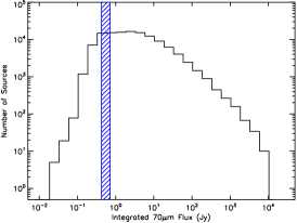
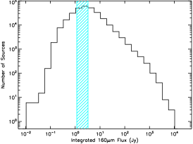
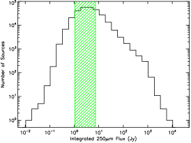
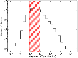
Figure 13: Histograms of the Integrated Flux F_Int for all Hi-GAL compact sources in the 5 bands for the entire DR1 Survey area. Flux completeness limits vary with Galactic Longitude (see fig. 9); the spanned longitude range (with the exception of the central —$l$—$\leq 2$^∘) is reported by the the colour-coded and shaded areas in fig. 9.

4.6 Photometric Corrections to Integrated Fluxes

The flux of the source candidates is derived from the parameters of the 2D-Gaussian fit found with CuTEx. While a 2D Gaussian is a good and acceptable approximation for the PSF of SPIRE (SPIRE Instrument Team & Consortium, 2014), the same is not true for PACS due to the observing setup adopted for the Hi-GAL survey. The on-board coaddition (in groups of 8 frames at 70$\mu$m and 4 frames at 160$\mu$m) while scanning the satellite, results in substantially elogated beams (see §2 above) that show significant departures from a circularly symmetric morphology. Part of this asymmetry is mitigated by the coaddition of scans in orthogonal directions, but significant departures from an ideal Gaussian symmetry persist. It is then necessary to estimate correction factors to be applied to the extracted CuTEx photometry to account for the (incorrect) assumption of Gaussian source brightness profiles assumed by CuTEx.

We adopted an empirical approach to estimate the corrections to the CuTEx photometry of PACS images. This was done by performing CuTEx photometry, using the same settings as used for the Hi-GAL catalogues, on an image of a primary Herschel photometric calibrator - $\alpha\leavevmode\nobreak\ Bootis$. $\alpha\leavevmode\nobreak\ Bootis$ was observed during OD 269 in the same conditions as the Hi-GAL observations (i.e. with two mutually orthogonal scan maps in parallel mode with a scanning speed of 60″/s). The $\alpha\leavevmode\nobreak\ Bootis$ images present a nice and clean point-like object with no detectable diffuse emission background (ideal photometry conditions compared to Hi-GAL). To extend the photometric correction factors to the more general case of compact but resolved sources, we convolved the images of $\alpha\leavevmode\nobreak\ Bootis$ with a 2D-circular Gaussian kernel of increasing size while normalizing integrated flux (i.e. flux conserving). The convolving kernels span the interval [0.0,5.0]$\times\theta_{0}$ in steps of 0.5$\theta_{0}$, where $\theta_{0}$ is the FWHM derived from the unconvolved $\alpha\leavevmode\nobreak\ Bootis$ profile. CuTEx integrated fluxes for the entire set of simulations were then compared with the expected values in the PACS bands as derived from theoretical models (Müller et al., 2014). After applying a colour correction estimated via Pezzuto et al. (2012), the fluxes of $\alpha\leavevmode\nobreak\ Bootis$ used for the comparison are 15.434 and 2.891 Jy at 70 and 160$\mu$m, respectively. Figure 12 reports the correction factors as estimated from the above analysis as a function of the FWHM of the compact source considered. The correction factors decrease rapidlyfrom point-like to minimally resolved sources. With larger sources, the decrease in the correction factor is a weaker function of source size. Beam asymmetries, however, are clearly persistent and detectable even for relatively extended sources.

The integrated fluxes for each source in the 70 and 160$\mu$m catalogues were corrected using the curves in fig. 12 and the sources’ circularised size (see§5.3). Both the uncorrected and the corrected integrated fluxes are reported in the columns FINT and FINT_UNCORR of the source catalogues (see Appendix A). We emphasise that these correction factors are only valid for images obtained from two scan maps taken in orthognal directions in pMode with a 60^′′/s scanning speed, and for sources extracted using a 2D Gaussian source model (i.e., they are not valid if PSF-fitting or aperture photometry is performed). The same analysis was carried out for SPIRE, but the correction factors estimated were largely within 10% for the unconvolved $\alpha\leavevmode\nobreak\ Bootis$ image, confirming the reliability of the Gaussian approximation for the SPIRE beams. Larger sources could not be simulated due to the high spatial density of background compact objects of extragalactic origin but, as suggested by fig. 12, the effect should be even lower.

5 Properties of the Compact Source Catalogues

5.1 Source fluxes and reliability

In fig. 13 we report the distribution of the integrated fluxes of all extracted compact sources in the 5 photometric bands. The histograms report the sources detected within the entire DR1 survey area. The large spread in detected fluxes, while representative of the entire survey, does not necessarily reflect the flux distribution in any individual tile. For example, the sources in the faint tail of the distributions originate mainly from the tiles at larger longitudes and are not detected in tiles like the one at $[l,b]$=(19^∘, 0^∘) for which we report the completeness limits in fig. 8, or from regions that are removed from the central latitude band around $b=0$^∘. In addition, the objects at the far left side of each histogram (low flux) are those that are potentially most affected by false positives, as dicussed in §4.2. We note, however, that even if we combine the sources in the 4 left-most bins of each histogram in fig. 13, these souces, combined, only account for 0.8% of the total number of sources in the 70$\mu$m band and less than 0.1% for the other bands.

It is difficult to identify a parameter that can be uniquely taken as a measure of the reliability of a source detection. It is important to remember that the background conditions found at Herschel wavelengths in the Galactic Plane are totally unprecedented. Therefore, criteria based on e.g. the S/N of the detected sources (that are reliable criteria in conditions of absent or low background) are not straightforward to apply, because compact sources have a variety of sizes (see §5.3) and sit on a Galactic ISM background that shows spatial variations at all scales. Fig. 14 illustrates the relationship between the background-subtracted peak flux densities of the sources and the intensity of the underlying background emission as estimated during the 2D Gaussian fitting in CuTEx. A direct relationship between the two quantities is apparent in all bands and Fig. 14 further shows that the peak flux of the sources is always a factor of a few fainter than the value of the background. An additional problem is that, not only does the background dominante over the source peak fluxes, but its fluctuations increase with the absolute level of the background. Therefore, since the uncertainties in the extracted source fluxes are computed starting from the residuals obtained after subtracting the fitted source+background (the latter modelled with a 2^nd-order surface) from the original maps, the magnitude of the residuals will be higher the higher the absolute level of the background. This is shown in fig. 15 where the r.m.s. of the fitted residuals is reported for the various bands as a function of the absolute level of the fitted background.

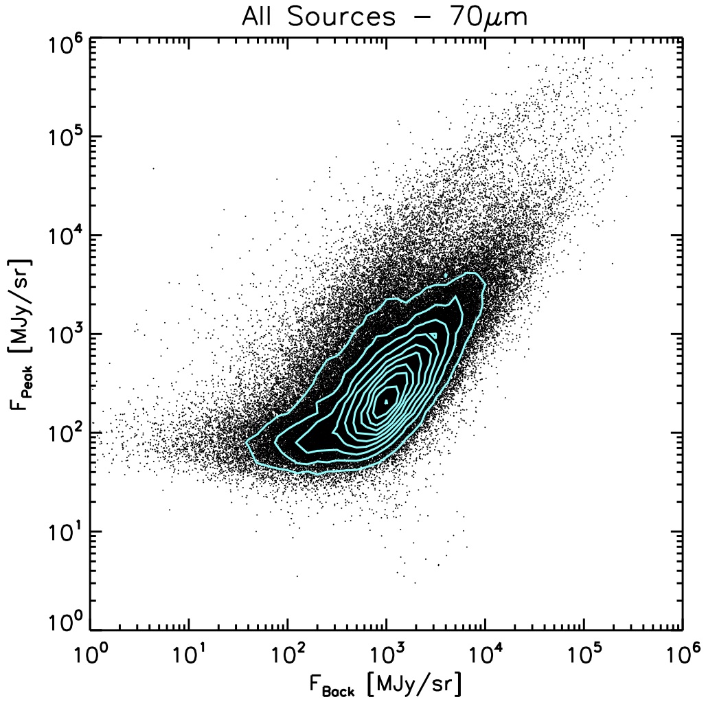
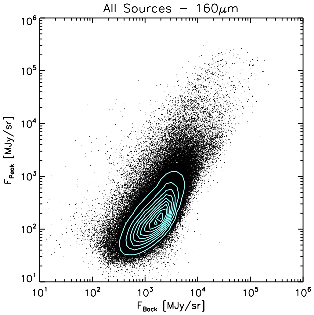
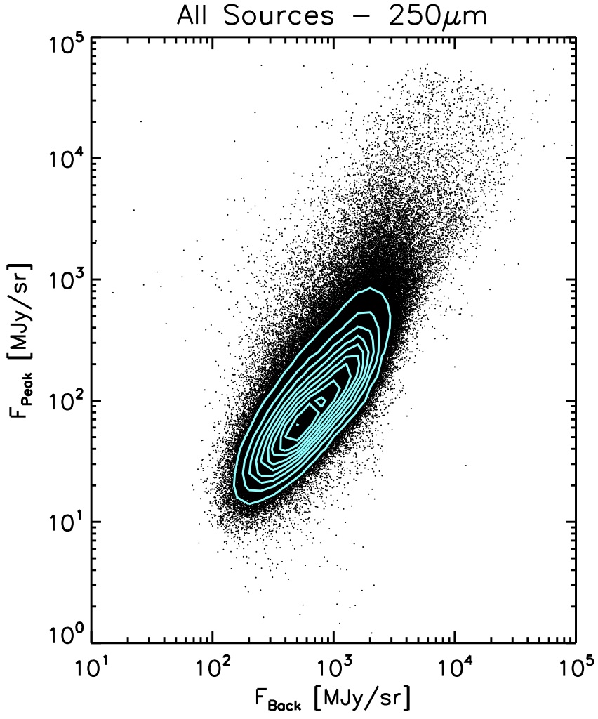
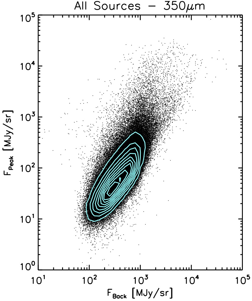
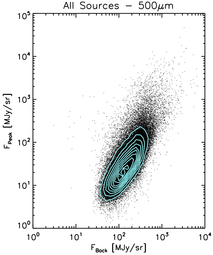
Figure 14: Plots of the background-subtracted source peak flux density F_Peak as a function of the flux density of the underlying background F_Back, as estimated by the source fitting for all Hi-GAL bands as indicated. The 10 cyan contours (equally spaced in source density) indicate the source density in the most crowded area. Note that axis scale is not the same in all panels.

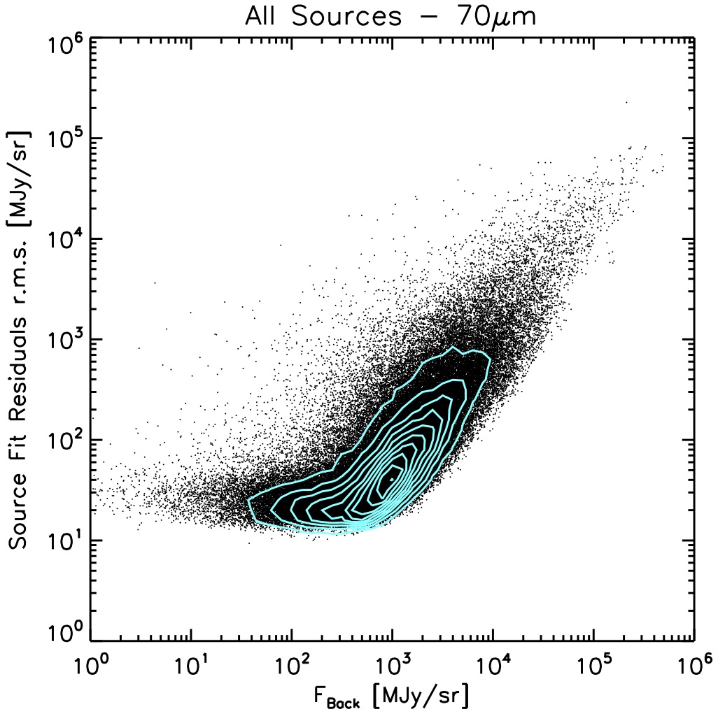
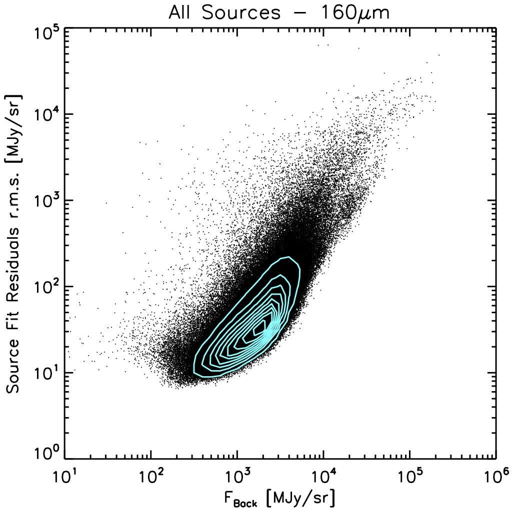
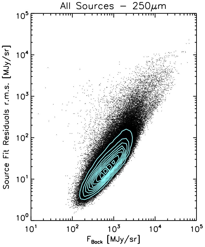
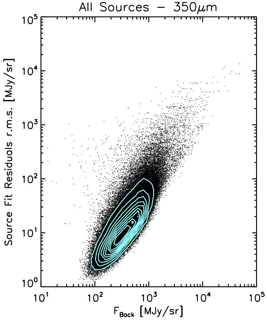
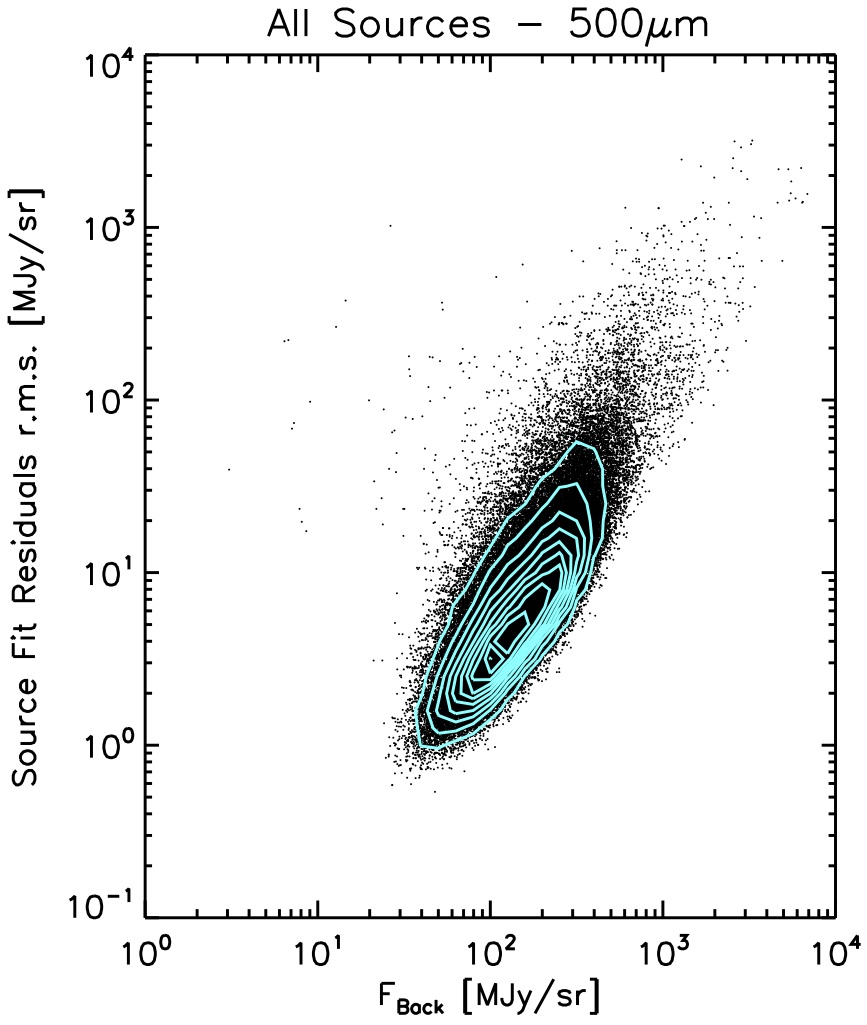
Figure 15: Plots of the r.m.s.of the flux density residuals after subtraction of the fitted source+background, as a function of the flux density of the underlying background F_Back, as estimated by the source fitting for all Hi-GAL bands as indicated. The 10 cyan contours (equally spaced in source density) indicate the source density in the most crowded area. Note that axis scale is not the same in all panels.

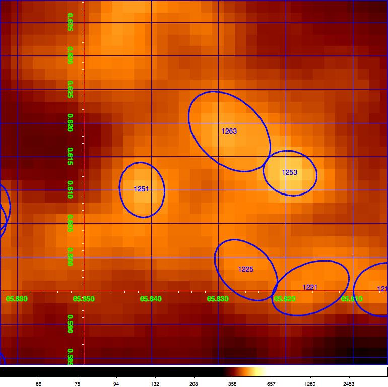
Figure 17: a (left panel) ) Case of a source at 250$\mu$m, labeled as # 117, in which the peak/background contrast is $\sim 1$ (hence relatively high, see fig.14) but the SNR is only 2.1. b (right panel) ) Case of a source at 250$\mu$m, labeled as #1251, with a very good SNR of 13.5, but with peak/contrast ratio $\sim 0.15$.

The result is that even relatively very bright objects will have a limited S/N. We plot in Fig. 16 the relationship between the integrated fluxes and their uncertainties. These uncertainties are the estimated r.m.s. of the image residuals computed by subtracting the source as fitted, and integrating the residual over the source’s fitted area. We see that a large majority of the extracted sources have SNR$\geq 3$ (the blue line in the figure), but rarely does the SNR go above $\sim 10$. This is the effect of the complex background that makes it difficult to estimate source sizes or even to effectively represent, in analytical form, the underlying background during the source fitting process. Therefore, it is possible that even relatively good contrast sources may have low SNRs. For example, Fig. 17a shows source #117 in the 250$\mu$m band which has a peak/background contrast of $\sim 1$ (which is relatively high compared to the average conditions represented in fig. 14) but whose SNR is only $\sim 2$. Yet, upon visual inspection, the source detection appears entirely reliable. This reinforces the notion that the quoted uncertainties should not be taken as a direct indication of the reliability of a source detection, but solely of the reliability of the estimated integrated flux. In other words, it may be difficult to estimate a high-fidelity flux even in the case of a bright source, given the intensity and complexity of the background found in the far-IR in the Galactic Plane.

One could be tempted then to adopt contrast value as a simple-to-use quality indicator for the reliability of a source. Unfortunately there are also several cases where relatively low contrast sources have high SNRs. This is demonstrated in fig. 17b, where source #1251 has a contrast of $\sim$0.15 but a SNR$\sim$13.5. Therefore, for the present release, we find ourselves in the very difficult situation where it is not possible to define any combination of parameters that may offer a reliable ”quality flag” for all detected sources. We therefore issue this first release of the Hi-GAL catalogues with a strong caveat; for the moment there is no easy shortcut to identify the most reliable sources other than attempting combinations of various parameters (that likely may give good results in certain background conditions but bad results in others) followed by visual inspection of the maps. A blind selection of sources with high SNR will definitely result in reliable samples, but will certainly miss many reliable objects.

A helping hand in this respect may come from cross-matching sources in different bands. The green points in Fig. 16 represent the subset of all sources for which a counterpart can be positionally matched (see Elia et al. 2016; Martinavarro-Armengol et al. 2015) in at least two adjacent wavelength bands. The fact that virtually all the green points are above the SNR=3 line is an indication that a positive match with counterparts in other bands is, at present, likely the best criterion to ensure the reliability of both the detection and the flux estimate for a source. Several sources that appear with high S/N at 70 and 160$\mu$m in fig. 16 do not show counterparts in at least three Hi-GAL bands (i.e. the black dots above S/N=3). For the greater part, these sources have relatively strong counterparts at shorter wavelengths and exhibit SEDs that decrease longward of 100$\mu$m and are not detected at SPIRE wavelengths. More complete statistics in this respect will be presented by Elia et al. (2016) and Martinavarro-Armengol et al. (2015) who will discuss the Hi-GAL photometric catalogues in the context of ancillary photometric Galactic Plane surveys like ATLASGAL (Schuller et al., 2009), MIPSGAL (Carey et al., 2009) and others. We emphasize once more that some of the sources with SNR$\geq 3$ and with counterparts in three adjacent bands (the green points) have integrated fluxes below the completeness limit pertinent to the specific Galactic longitude if the source is located more than 0.3-0.4 degrees latitude on average off the midplane.

As experience accumulates in the use of these catalogues we plan to improve the quality assessment for the catalogue sources in subsequent data releases. Ultimately, since there may be no better instrument to judge the reliability of a source than an astronomer’s trained eye, a possible strategy could be to deploy machine-learning capabilities. In such techniques, input from a trained user would teach the algorithm to look for specific patterns in the combination of catalogue parameters, thereby allowing it to automatically identify sources that should be discarded.

5.2 Contamination from extra-galactic sources

Although the Galactic Plane is inarguably the most unfavourable environment in which to detect galaxies, there is no doubt that background galaxies could, in principle, contaminate the detection of Galactic sources in Galactic Plane surveys (Marleau et al., 2008; Amores et al., 2012). To evaluate the degree of possible contamination from galaxies in our photometric catalogues, we take advantage of the shallow cosmological surveys carried out by Herschel using the same observing mode that we used for Hi-GAL. Rigby et al. (2011) report the photometric catalogues for the Science Demonstration Phase fields of the H-ATLAS survey with SPIRE (Eales et al., 2010), showing that at 250$\mu$m the density of extragalactic sources with integrated flux larger than 0.1 Jy is of the order of 10 deg^-2. The distribution of the integrated fluxes in the 250$\mu$m Hi-GAL catalogues reported in fig. 13 shows that basically all (99.98%) of the $\sim 280\,000$ sources detected at 250$\mu$m have fluxes above 0.1 Jy; as the present catalogue release encompasses a surveyed area of $\sim 270$ square degree, the average density of the 250$\mu$m Hi-GAL sources is therefore $\sim$1000 deg^-2. The average contamination from extragalactic sources is, therefore, $\leq$1% at 250$\mu$m. Using the same method, the contamination fractions at the other SPIRE wavelengths are $\leq$ 0.7% at 350$\mu$m and $\leq$ 0.3% at 500$\mu$m. Given the shape of extragalactic source counts Rigby et al. (2011), these estimated contaminations are concentrated toward the faint end of the Hi-GAL source catalogues. The extragalactic source density decreases by 1 order of magnitude going from 0.1 to 0.4 Jy, while the number of Hi-GAL 250$\mu$m sources above 0.4 Jy is still 99.3% of the total. Therefore, contamination effect from extragalactic background sources is negligible and limited to integrated fluxes below 0.4Jy at 250$\mu$m. The situation is even more favourable at the other SPIRE wavelengths. This is marginally visible in the histograms of Fig. 13.

Concerning the PACS bands, Lutz et al. (2011) provide photometric catalogs from the PEP program which surveyed well-known consmological fields. About 125 sources with fluxes above 0.1Jy at 160$\mu$m are detected in the 2.78 sq. deg. PEP fields, corresponding to about 45 deg^-2. Using the same approach as for the SPIRE bands, this corresponds to a contamination fraction from extragalactic sources of the order of 4%. However, the PEP PACS maps were taken in Prime Mode with a scan speed of 20^′′/s, achieving much higher sensitivities than in Parallel Mode observations, especially in the virtually background-free conditions typical of cosmological fields. Lutz et al. (2011) quote 3$\sigma$ noise levels of 8 mJy, which agrees very well with the expected noise levels predicted by the HSpot tool for the PEP observing mode at the centre of the maps where the coverage is higher. On the other hand, the HSpot tool provides a 1$\sigma$ sensitivity of $\sim$46 mJy at 160$\mu$m for observations in Parallel Mode, or a factor $\sim$16 worse than for observations in Prime Mode. If we artificially degrade the flux uncertainties reported by Lutz et al. (2011) by this factor, the number of sources that would have been detected at a 3$\sigma$ level would decrease from 125 to 29, bringing the contamination level down to $\leq$1%. PEP 70$\mu$m source catalogues have been made available for the GOODS-S field only (Lutz et al., 2013), and only 1 source has been detected with a flux greater than 0.1 Jy, which is not a large enough sample with which to assess possible contamination. Given this single detection, however, we deem the contamination to be negligible in this band.

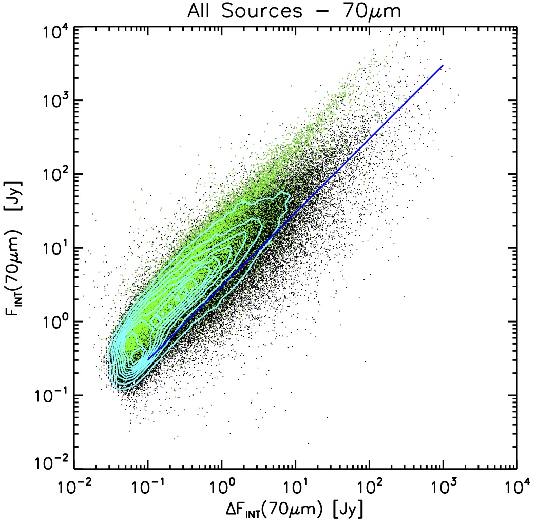
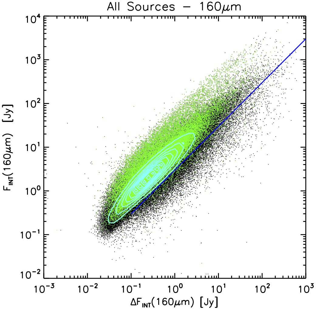
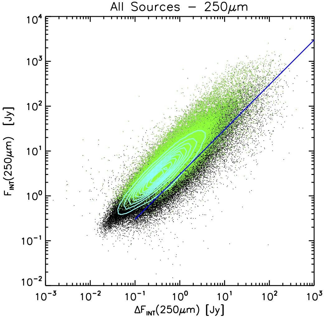
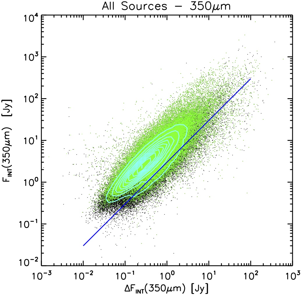
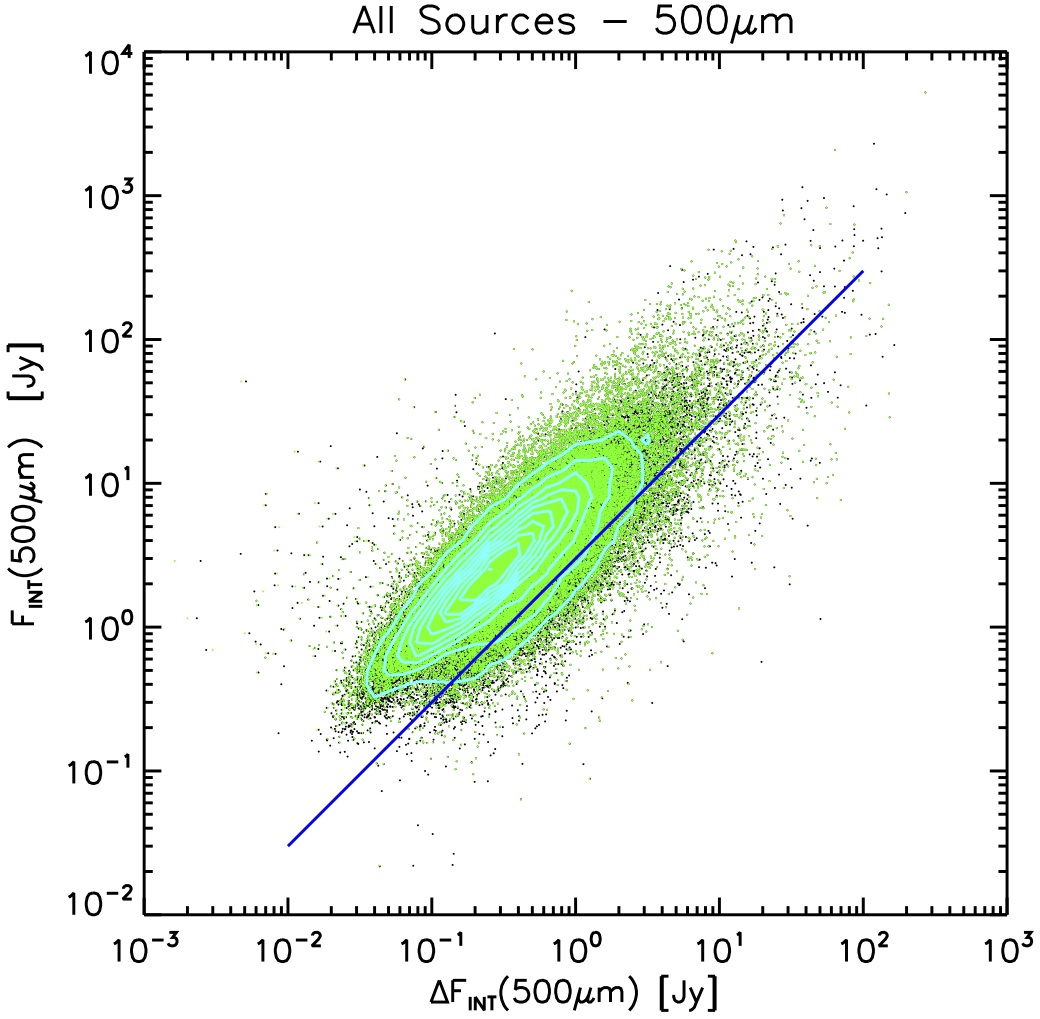
Figure 16: Plots of the Integrated Flux F_Int as a function of its uncertainty $\Delta$F_Int for all Hi-GAL bands as indicated. The black points are all the sources in each band catalogue; the 10 cyan contours (equally spaced in source density) indicate the source density in the most crowded area. The green points are the subset of sources that possess a counterpart in at least two adjacent bands (so as to form an SED with at least three photometric points, see Elia et al. 2016). The blue line represents SNR_Int=3.

We conclude that contamination from distant background galaxies is extremely low and concentrated toward the faint end of the flux distribution of the Hi-GAL sources. This effect is, perhaps, visible in Fig. 13 as a tentative flattening of the flux distributions at F${}_{int}\leq$0.1 Jy for the 160, 250 and 350$\mu$m bands. Local universe galaxies have larger fluxes, but are also far from compact and have a very low spatial density (see Ciesla et al. (2012) and Boselli et al. 2010) Therefore, it is unlikely that they have been included in the present catalog.

5.3 Source sizes

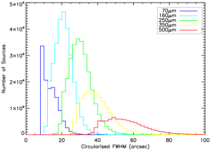
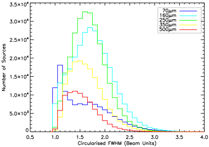
Figure 18: Top-panel) Distribution of the circularized FWHM of the catalogue sources in the five bands. Sizes are computed as the geometric mean of the FWHMs estimated by 2D Gaussian fitting in two orthogonal directions. Bottom-panel) Same as above, but in units of the beam-size.

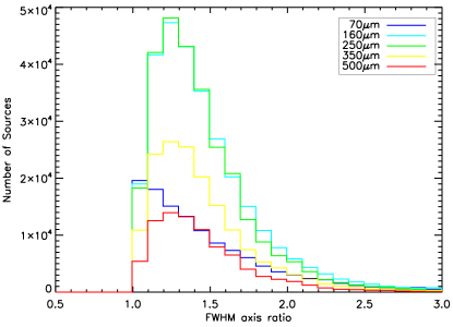
Figure 19: Distribution of the axis ratio, computed as the ratio of FWHM_Maj/FWHM_min of the catalogued sources in the five bands.

Fig. 18 reports the distribution of the circularized source sizes in the different bands, calculated by taking the square root of the product of the major and minor axis as estimated by CuTEx. Source sizes span a range of values, from that of the PSF to about twice the PSF for most of the sources. The broad distributions in Fig. 18 show that the sources are generally mildly resolved, with the exception of the 70$\mu$m band where a peak at the PSF value is clearly visible. We stress that Fig. 18 reports the circularised sizes; sources may be unresolved in one direction and resolved in the other, therefore resulting in being moderately resolved on average. This is confirmed by Fig. 19 showing that extracted sources are mildly elliptical, with axis ratios peaking between 1.2 and 1.3, and with the large majority of the sources showing values below 1.5.

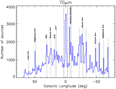
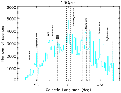
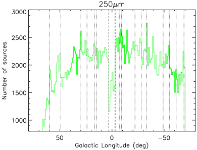
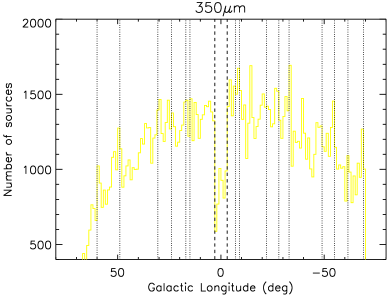
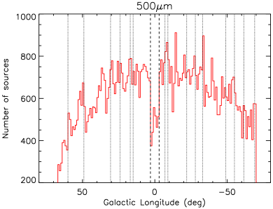
Figure 20: Longitude distribution of source counts (in 1^∘ bins) at 70, 160, 250, 350 and 500$\mu$m colour-coded as in fig. 9. The vertical dashed lines denote the longitude range close to the Galactic centre where SPIRE was used in “bright source” mode to avoid saturation and non-linearities in detector response. Labeled dotted lines indicate major spiral arms, tangent point/intersections or star forming complexes.

It is not surprising to find such a low number of PSF-like sources in the Hi-GAL catalogues. Compact dust clumps around young star forming objects do not show abrupt transitions in density when they merge into the ISM filaments or clouds in which they are embedded, so there is no reason a priori to expect these objects to be unresolved. The physical size of dense clumps hosting protoclusters, on average between 0.1 and 1 parsecs, should indeed be resolvable for a large span of heliocentric distances with the angular resolutions accessible to the Herschel cameras. This aspect will be discussed in more detail in Elia et al. (2016). On the other hand, it has been noted several times that the intensity of extended emission background in the DR1 Hi-GAL maps is generally higher (fig. 14) than the peak flux of the detected compact sources. The ideal flat and faint background conditions of the $\alpha$ Boo image that was used in §4.6 to calibrate the departures of the brightness profile for point-like and mildly extended compact sources, are never found on the Galactic Plane at Herschel wavelengths, with the exception of some spots in the most peripheral tiles at 70$\mu$m . Under these conditions, it is certainly difficult for any adaptive brightness profile-fitting algorithm to converge to PSF-like source sizes.

6 Global properties of the Galactic structure.

Figure 20 shows the distribution of Hi-GAL sources in Galactic longitude for the five wavelength bands. All histograms show decreasing source counts as a function of distance from the Galactic Centre, comparing very well with similar plots from other infrared and submillimetre surveys. A variety of peaks can be seen throughout the longitude range, with greater dynamic range for the 70 and 160$\mu$m bands. The abrupt dips in source count over the 6^∘-wide region centred on the Galactic centre which are clearly visible in the SPIRE bands is due to the fact that SPIRE was used in “bright source” mode for the three tiles of the survey close to the Galactic Centre (see §2).

Similar to Beuther et al. (2012) we identify on fig. 20 features that can be associated with major star formation complexes or to source accumulations along the line of sight correspondening to tangent points or major intersections of the line of sight with known spiral arms.

A comparison with the ATLASGAL survey (Schuller et al., 2009), covering the Galactic Plane between roughly +60^∘and $-60$^∘in the 870$\mu$m continuum, shows substantial similarities in the source count distributions, confirming that both surveys are mostly tracing dense, star-forming (or potentially star-forming) regions. A similar distribution was also found by Rygl et al. (2010) using high-extinction clouds identified with Spitzer colours excess Therefore, it is reasonable to posit that ATLASGAL is typically tracing the higher-flux fraction of the Hi-GAL sources, although this depends on the intrinsic SEDs of the various objects. We defer a detailed analysison on this topic to a subsequent paper (Elia et al., 2016). .

The latitude distribution of the Hi-GAL compact sources is reported in fig. 21 for the 70$\mu$m and the 250$\mu$m catalogue sources. Both histograms peak at slightly negative values, similar to what was recently reported for the ATLASGAL submillimetre sources distribution as well as for other infrared and molecular line data Galactic plane surveys (see Beuther et al. 2012 and references therein). The median values for Hi-GAL source latitude is $\sim-$0^∘.06 below the nominal midplane, in excellent agreement with the value reported for ATLASGAL by Beuther et al. (2012). We therefore confirm that the current definition of the Galactic midplane may need to be revisited to account for a latitude shift that most likely reflects an overall bias; possibly due to an incorrect assumption of the Sun’s vertical position in the Milky Way. A more in-depth and statistically significant analysis of the latitude distribution of the Hi-GAL sources as a function of longitude is deferred to a companion paper (Molinari et al., 2015).

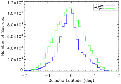
Figure 21: Distribution of Galactic latitude values for the Hi-GAL sources with F${}_{Int}\geq$0.5Jy at 70$\mu$m (blue line), and with F${}_{Int}\geq$3.0Jy at 250$\mu$m (green line).

7 Conclusions

This is the first public Data Release of high-quality products from the Herschel Hi-GAL survey. The release comes 2 years after the end of the Herschel observing, and is the result of extensive testing of the data reduction and extraction procedures created by members of the Hi-GAL Consortium. The complexity and the large variation of the background conditions in all Herschel wavelength bands makes source extraction on the Galactic Plane a non-trivial task. With Hi-GAL DR1, we provide access, via a cutout service, to high-quality images and Compact Source Catalogues for the Galactic Plane at 70, 160,250, 350 and 500$\mu$m in the region 68^∘$\gtrsim l\gtrsim-70$^∘ and $|b|\leq 1$^∘. the service is accessible from the VIALACTEA Project portal at http://vialactea.iaps.inaf.it.

The catalogues were generated using the CuTEx software package that was specifically designed to operate in the intense and highly spatially variable background conditions found in the Galactic Plane at Far-infrared wavelengths. Source detection is carried out on the 2^nd-derivative of the brightness images which is particularly sensitive to curvature in the continuum brightness spatial distribution. The detection is optimised for compact objects with FWHM typically ranging from 1 to three times the instrumental PSF(but mostly within 2 times the PSF). The impact of false positives is estimated, and a careful analysis of the flux completeness limits is presented, independently for each photometric band. The source catalogues contain 123210, 308509, 280685, 160972 and 85460 sources in the five bands, respectively.

After considerable time, effort and experience gathered through use of the photometric calatogues by Hi-GAL Consortium astronomers, we are not yet at a stage where we feel we can confidently define a figure of merit that can uniquely and definitively be used to assess the degree of reliability of a source detection. Thresholding on the S/N ratio that we assign to each source appears to be the best way to select bona fide compact objects. Although the user should be warned that, due to the complex background conditions, there may be sources with a formal S/N$<$3 that have relatively good contrast ratios over the background and appear reliable on visual inspection. An additional crriterion to assess the reliability of sources is their persistence in other adjacent photometric bands.

Subsequent releases are planned that will cover the entire Galactic Plane, with even higher quality catalogues based on improved handling of the problems present in source extraction for variable-size objects in extreme background conditions. Additional products will include carefully intercalibrated large map mosaics and dust column density maps.

Appendix A Explanatory note for the Hi-GAL photometric catalogs

Table 3: Field description for the single-band photometric catalogs.

Field name	Format	Units	Description
Source identification and position information
DESIGNATION	A25	$-$	Designation of the source based on its Galactic position in the form LLL.llll$\pm$b.bbbb. The naming convention for the Hi-GAL cataloguehas the form HIGALPXLLL.llll$\pm$b.bbbb, where HIGALP stands for the preliminary catalog, X stands for the band where the source has been identified among the possible choices: B - blue band; R - red band; S - PSW band; M - PMW band; L - PLW band.
GLON	F12.6	degrees	Galactic longitude of the source
GLAT	F12.6	degrees	Galactic latitude of the source
DGLON	F5.2	arcsec	Uncertainty in the Galactic longitude coordinate derived from the fitting procedure. 0 indicates that the fitting process hit the boundary limits imposed to the fit.
DGLAT	F5.2	arcsec	Uncertainty in the Galactic latitude coordinate derived from the fitting procedure. 0 indicates that the fitting process hit the boundary limits imposed to the fit.
RA	F12.6	degrees	J2000 Right Ascension for the source
DEC	F12.6	degrees	J2000 Declination for the source
ATLAS_IMAGE	A40	$-$	Atlas Image file identifier from which source was extracted.
X	F9.3	pixel	x-pixel coordinate of this source on the original image.
Y	F9.3	pixel	y-pixel coordinate of this source on the original image.
DX	F9.3	pixel	Uncertainty in the x coordinate of this source derived from the fitting procedure.
DY	F9.3	pixel	Uncertainty in the y coordinate of this source derived from the fitting procedure.
SOURCE_ID	A10	$-$	Unique source identification in the form lLLL NNNN, where lLLL is a unique identifier of the original image over which source extraction was carried out, and NNNN is a progressive 4 digit, zero-filled, number indicating the sequential order of extraction.
Primary Photometric information
FINT_UNCORR	F15.3	Jy	Source Integrated flux measured from the fitting process
FINT	F15.3	Jy	Source Integrated flux measured from the fitting process after applying photometric corrections as a function of the source size, to account for source non-Gaussianity and for scan speed.
ERR_FINT	F15.3	Jy	Uncertainty on the integrated flux computed by multiplicating the fitted source residual r.m.s. (RMS_TOTAL) by the fitted source area as estimated by FWHMA and FWHMB.
FPEAK	F15.3	MJy/sr	Source peak flux measured from the fitting process
FWHMA	F10.2	arcsec	Full Width Half Maximum of the source along axis $a$ of the elliptical Gaussian as determined by fitting engine.
FWHMB	F10.2	arcsec	Full Width Half Maximum of the source along axis $b$ of the elliptical Gaussian as determined by fitting engine.
PA	F6.1	degrees	Position angle of the elliptical Gaussian (N$\rightarrow$E).
BACKGROUND	F15.3	MJy/sr	Background value determined at the source peak position.
BACK_ACOEFF	F12.5	MJy/sr	Coefficient a of the 0th-order term of the background obtained by the fit at the source peak position.
BACK_BCOEFF	F12.5	MJy/sr/pxl	Coefficient b of the 1th-order term $x$ of the background obtained by the fit at the source peak position.
BACK_CCOEFF	F12.5	MJy/sr/pxl	Coefficient c of the 1th-order term $y$ of the background obtained by the fit at the source peak position.
BACK_DCOEFF	F12.5	MJy/sr/pxl2	Coefficient d of the 2nd-order term $x^{2}$ of the background obtained by the fit at the source peak position.
BACK_ECOEFF	F12.5	MJy/sr/pxl2	Coefficient e of the 2nd-order term $y^{2}$ of the background obtained by the fit at the source peak position.
BACK_FCOEFF	F12.5	MJy/sr/pxl2	Coefficient f of the 2nd-order term $xy$ of the background obtained by the fit at the source peak position.
RMS_TOTAL	F12.5	MJy/sr	Standard Deviation, $\sigma_{loc}$, of the residuals computed within the source area defined by FWHMA and FWHMB after the subtraction of the best fit.
RMS_SURROUND	F12.5	MJy/sr	Standard Deviation, $\sigma_{loc}$, of the residuals computed within the fitting window after the subtraction of the best fit, excluding both the pixels that belong to the source and the pixels belonging to other sources that fall within the fitting window.
SNR	F12.5	$-$	Signal-to-noise ratio obtained by dividing FPEAK by the residual r.m.s. over a source area with FWHMA and FWHMB as semi-axes .
Basic detection information
DET_X	F10.3	$-$	Relevance of the source in the 2nd derivative map along $x$-axis defined as the ratio between the measured 2nd derivative at source peak position and the adopted local threshold value
DET_Y	F10.3	$-$	Relevance of the source in the 2nd derivative map along $y$-axis defined as the ratio between the measured 2nd derivative at source peak position and the adopted local threshold value

Table 3: Continued

Field name	Format	Units	Description
Basic extraction information
DET_X45	F10.3	$-$	Relevance of the source in the 2nd derivative map along the bisector of the $xy$-axis defined as the ratio between the measured 2nd derivative at source peak position and the adopted local threshold value
DET_Y45	F10.3	$-$	Relevance of the source in the 2nd derivative map along the bisector of the $yx$-axis defined as the ratio between the measured 2nd derivative at source peak position and the adopted local threshold value
DETLIM_X	F10.3	MJy/sr/pxl2	Absolute value for the local detection limit threshold adopted for the 2nd derivate along the $x$-axis coordinate
DETLIM_Y	F10.3	MJy/sr/pxl2	Absolute value for the local detection limit threshold adopted for the 2nd derivate along the $y$-axis coordinate
DETLIM_X45	F10.3	MJy/sr/pxl2	Absolute value for the local detection limit threshold adopted for the 2nd derivate along the bisector of the 1st and 3rd quadrant.
DETLIM_Y45	F10.3	MJy/sr/pxl2	Absolute value for the local detection limit threshold adopted for the 2nd derivate along the bisector of the 2nd and 4th quadrant.
CLUMP_FLAG	I5	$-$	Flag for confusion at detection level. A value equal to 0 means that the source was identified from an isolated group of pixels above the threshold in all the four derivative directions. Sources belonging to the extraction of the same Atlas Image having the same value of this flag belong to the same group of pixels above the threshold.
NCOMP	I2	$-$	Number of gaussian components used simultaneously in the fitting process. This number includes the source, so the minimum value is 1, such number is greater than 1 if the source is fit with other nearby detections.
XCENT	F9.1	pxl	The $x$-pixel coordinate of the centre of the source fitting window on the original image.
YCENT	F9.1	pxl	The $y$-pixel coordinate of the centre of the source fitting window on the original image.
XWINDOW	I2	pxl	Half-width size of the source fitting window along $x$ coordinate and centred at XCENT.
YWINDOW	I2	pxl	Half-width size of the source fitting window along $y$ coordinate and centred at YCENT.
NCONTAM	I2	$-$	Number of other sources falling inside the fitting window whose presence is taken into account at fitting stage. Not all those other sources might have been fitted at the same time
CENT_TOL	F5.2	pxl	Maximum variation in pixels for adjustment of the fit centre with respect to the position of detection, measured as the distance between the latter and the brightest local (withing 3-pixel) pixel in the fitting window.
DOF	I4	$-$	Degrees of freedom of the source Gaussian fit.
Quality Flags
CHI2	F12.5	$-$	$\chi^{2}$ determined by the fitting engine.
CHI2_OPP	F12.5	$-$	Estimator of the fidelity between the fit and the data computed as $\phi$= (O(i) - F(i))2 / F(i), where O(i) is the observed data in the i pixel of the fitting window and F(i) is the fitted value in the same position
FIT_STATUS	I1	$-$	Flag returned from the fitting engine. Possible values of the flag are: 0 - Fit convergence failed; 1 - Convergence reached; 2 - Convergence reached despite the initial accurary requested to fitting engine was set too low; 3 - Maximum number of iterations in the fitting process reached; 4 - Problems in Fitting due to the initial guess.
GUESS_FLAG	A3	$-$	Flag on quality of guessed source parameters as determined at the detection stage. The form of the flag is GN where G is a letter defined as: A - Optimal number of positions to estimate the size; B - Sufficient number of positions to estimate the size; C - Low number of positions to estimate the size; and N is a number defining the quality of inital guess size: 0 - Initial Estimate failed; 1 - Good initial estimate for sizes; 2 - One of the two guessed sizes was initially estimate as smaller of PSF; 3 - Initial estimates of source sizes were larger than 3 times the PSF
GROUP_FLAG	I5	$-$	Flag on quality of guessed source parameters as determined at the detection stage. The form of the flag is GN where G is a letter defined as: A - Optimal number of positions to estimate the size; B - Sufficient number of positions to estimate the size; C - Low number of positions to estimate the size; and N is a number defining the quality of inital guess size: 0 - Initial Estimate failed; 1 - Good initial estimate for sizes; 2 - One of the two guessed sizes was initially estimate as smaller of PSF; 3 - Initial estimates of source sizes were larger than 3 times the PSF
CONSTRAINTS	I1	$-$	Flag indicating the number of parameters that reached the tolerance limits allowed to the fit process. Values as 4 indicate that the source flux has higher unreliability since either the centre and its sizes have reached the maximum (or the minimum) allowed for the fit engine
SHIFT_FLAG	F9.3	arcsec	Amount of shift of the source peak position from its original detection position, due to Gaussian fitting.

Table 3: Continued

Field name	Format	Units	Description
Basic extraction information
RDETP2DX	F9.3	$-$	Ratio between the 2nd derivative value along $x$ direction expected by the fitted model of the source and the 2nd derivative derivative measureat the detection stage. Values closer to 1 indicate higher reliability of the source.
RDETP2DY	F9.3	$-$	Ratio between the 2nd derivative value along $y$ direction expected by the fitted model of the source and the 2nd derivative measureat the detection stage. Values closer to 1 indicate higher reliability of the source.
RDETP2DX45	F9.3	$-$	Ratio between the 2nd derivative value along the bisector of the $xy$ direction expected by the fitted model of the source and the 2nd derivative measureat the detection stage. Values closer to 1 indicate higher reliability of the source.
RDETP2DY45	F9.3	$-$	Ratio between the 2nd derivative value along the bisector of the $yx$ direction expected by the fitted model of the source and the 2nd derivative measureat the detection stage. Values closer to 1 indicate higher reliability of the source.
OVERLAP_FLAG	F9.3	$-$	Flag to indicate whether the source has been detected and extracted in one or more adiacent tiles. H indicates that the source has been detected in the tile named in column ATLAS_IMAGE; E,W indicate that the source is detected only in the eastern or western adiacent tile, respectively (east is higher galactic longitude); if the source has been detected in both H and E or W, then the name of the adiacent tile is also listed (e.g. H_l060). In those cases, the entry in the catalogue is the one with the highest SNR.
OVFLUX_FLAG	I	$-$	Flag to indicate which flux values were adopted if detected and extracted in two adiacent tiles. 0 indicates that the soruce has been detected only in once and therefore all fluxes refer to that detection. -1 indicates that the two fluxes differ by more than 15%; the one listed is that with the highest SNR. 1 indicates that both integrated fluxes lie within 15%, the one in the catalogue is that with highest SNR. 2 indicates that the integrated fluxes differ by more than 15% but FPEAK are within 15%; the one listed is that with highest SNR.

Appendix B Saturated pixels in Hi-GAL maps

Table LABEL:sat_tab reports the location of the clusters of saturated pixels in the Hi-GAL mapped area. The longitudes and latitudes in cols. 1-2 represent the centroid position of the cluster at the shortest wavelength where the saturation conditions exists. The subsequent 8 columns report for each band from 160 to 500 $\mu$m, the number of saturated pixels for each location and the radius of the circularized area of the saturated pixels cluster in arcseconds. The last column reports the sources from the IRAS Point Source Catalogue or from the RMS Source Catalogue that are located within 1^′ (for IRAS sources) and 40^′′ (for MSX sources), from the pixels cluster centroid.

Table 4: Clumps or clusters of saturated pixels, crossmatched with IRAS point sources, and RMS sources. IRAS sources $<60\arcsec$, RMS sources $<40\arcsec$ from cluster barycentre.

				red			PSW			PMW			PLW
Gal. Lon.	Gal. Lat.	Map		Pix.	$R_{e}$		Pix.	$R_{e}$		Pix.	$R_{e}$		Pix.	$R_{e}$		IRAS	RMS
($\degr$)	($\degr$)				(″)			(″)			(″)			(″)
291.26944	-0.71532	l290		-	-		67	27		1	4		-	-		11097-6102	-
291.57932	-0.43251	l290		-	-		7	8		-	-		-	-		-	G291.5765-00.4310
291.26944	-0.71508	l292		-	-		67	27		3	7		-	-		11097-6102	-
291.57941	-0.43112	l292		-	-		4	6		-	-		-	-		-	G291.5765-00.4310
301.13687	-0.22566	l301		-	-		18	14		3	7		-	-		12326-6245	G301.1364-00.2249
305.20917	0.20578	l305		-	-		8	9		-	-		-	-		13079-6218	G305.2017+00.2072A, G305.2017+00.2072B
305.35797	0.20391	l305		-	-		6	8		-	-		-	-		13092-6218	-
305.36215	0.15114	l305		-	-		3	5		-	-		-	-		-	-
305.36771	0.21224	l305		-	-		1	3		-	-		-	-		-	G305.3676+00.2095, G305.3779+00.2108
305.79990	-0.24385	l305		-	-		3	5		-	-		-	-		13134-6242	G305.7991-00.2461A, G305.7991-00.2461B
309.92188	0.47956	l310		-	-		2	4		-	-		-	-		13471-6120	G309.9206+00.4790A, G309.9206+00.4790B
311.62744	0.29010	l312		-	-		5	7		-	-		-	-		14013-6105	G311.6264+00.2897
314.21927	0.27282	l314		-	-		1	3		-	-		-	-		14214-6017	G314.2204+00.2726
316.81213	-0.05743	l316		-	-		3	5		-	-		-	-		14416-5937	G316.8112-00.0566
318.04984	0.08687	l319		-	-		1	3		-	-		-	-		14498-5856	G318.0489+00.0854A, G318.0489+00.0854B, G318.0489+00.0854C
318.94812	-0.19645	l319		-	-		1	3		-	-		-	-		-	G318.9480-00.1969A, G318.9480-00.1969B
322.15808	0.63623	l321		-	-		23	16		4	9		-	-		-	-
322.16376	0.62281	l321		-	-		13	12		-	-		-	-		-	-
322.15823	0.63590	l323		-	-		21	15		-	-		-	-		-	-
322.16400	0.62258	l323		-	-		7	8		-	-		-	-		-	-
323.74069	-0.26362	l323		-	-		5	7		-	-		-	-		15278-5620	G323.7399-00.2617A, G323.7399-00.2617B, G323.7410-00.2552A, G323.7410-00.2552B, G323.7410-00.2552C
324.20078	0.12143	l323		-	-		6	8		-	-		-	-		15290-5546	G324.1997+00.1192
324.20093	0.12056	l325		-	-		5	7		-	-		-	-		15290-5546	G324.1997+00.1192
326.47467	0.70227	l325		-	-		4	6		-	-		-	-		15394-5358	G326.4755+00.6947
326.65701	0.59368	l325		-	-		5	7		-	-		-	-		15408-5356	-
326.72165	0.61432	l325		-	-		1	3		-	-		-	-		15411-5352	G326.7249+00.6159A, G326.7249+00.6159B
326.65836	0.59550	l327		-	-		1	3		-	-		-	-		15408-5356	-
326.67001	0.55551	l327		-	-		1	3		-	-		-	-		-	G326.6687+00.5495
326.72278	0.61440	l327		-	-		3	5		-	-		-	-		15411-5352	G326.7249+00.6159A, G326.7249+00.6159B
327.29385	-0.57797	l327		-	-		38	20		17	18		3	11		-	G327.2852-00.5735
327.30011	-0.54923	l327		-	-		30	18		-	-		-	-		15492-5426	-
327.30661	-0.54101	l327		-	-		1	3		-	-		-	-		15492-5426	-
327.40240	0.44477	l327		-	-		4	6		-	-		-	-		15454-5335	G327.4014+00.4454
328.23657	-0.54683	l327		-	-		2	4		-	-		-	-		-	-
328.25488	-0.53147	l327		-	-		7	8		-	-		-	-		15541-5349	G328.2523-00.5320A, G328.2523-00.5320B, G328.2523-00.5320C
328.30728	0.43178	l327		-	-		7	8		-	-		-	-		15502-5302	G328.3067+00.4308
328.56671	-0.53409	l327		-	-		9	10		-	-		-	-		15557-5337	G328.5669-00.5327
328.57483	-0.53013	l327		-	-		2	4		-	-		-	-		15557-5337	G328.5669-00.5327
328.80792	0.63265	l327		2	3		32	19		8	12		-	-		15520-5234	G328.8074+00.6324
328.57144	-0.53254	l330		-	-		16	13		-	-		-	-		15557-5337	G328.5669-00.5327
328.80875	0.63335	l330		-	-		29	18		7	11		-	-		15520-5234	G328.8074+00.6324
329.02948	-0.20541	l330		-	-		3	5		-	-		-	-		15566-5304	-
329.18417	-0.31345	l330		-	-		2	4		-	-		-	-		15579-5303	-
329.33844	0.14789	l330		-	-		12	11		-	-		-	-		15567-5236	G329.3371+00.1469
329.40497	-0.45928	l330		-	-		1	3		-	-		-	-		15596-5301	G329.4055-00.4574
330.87857	-0.36690	l330		-	-		18	14		3	7		-	-		16065-5158	G330.8708-00.3715A, G330.8708-00.3715B, G330.8845-00.3721
330.95459	-0.18134	l330		7	6		32	19		13	16		-	-		16060-5146	G330.9544-00.1817
330.87854	-0.36711	l332		-	-		19	14		2	6		-	-		16065-5158	G330.8708-00.3715A, G330.8708-00.3715B, G330.8845-00.3721
330.95401	-0.18147	l332		-	-		33	19		12	15		-	-		16060-5146	G330.9544-00.1817
331.13147	-0.24311	l332		-	-		7	8		-	-		-	-		16071-5142	G331.1282-00.2436
331.27811	-0.18765	l332		-	-		1	3		-	-		-	-		16076-5134	G331.2759-00.1891B
331.51184	-0.10189	l332		-	-		15	13		-	-		-	-		-	G331.5131-00.1020, G331.5180-00.0947A, G331.5180-00.0947B
331.55585	-0.12044	l332		-	-		3	5		-	-		-	-		16086-5119	G331.5582-00.1206
332.09387	-0.42099	l332		-	-		2	4		-	-		-	-		16124-5110	G332.0939-00.4206
332.82730	-0.54833	l332		5	5		33	19		10	14		-	-		16164-5046	G332.8256-00.5498A, G332.8256-00.5498B
332.96378	-0.67754	l332		-	-		2	4		-	-		-	-		16175-5045	G332.9636-00.6800
333.06830	-0.44629	l332		-	-		9	10		-	-		-	-		-	G333.0682-00.4461
333.12161	-0.43240	l332		-	-		9	10		-	-		-	-		16172-5028	G333.1256-00.4367, G333.1306-00.4275
333.13354	-0.43052	l332		-	-		85	31		14	16		-	-		16172-5028	G333.1306-00.4275, G333.1256-00.4367
333.28455	-0.38667	l332		-	-		37	20		1	4		-	-		-	G333.2880-00.3907
333.29950	-0.35258	l332		-	-		1	3		-	-		-	-		16177-5018	-
332.82697	-0.54870	l334		-	-		31	18		9	13		1	6		16164-5046	G332.8256-00.5498A, G332.8256-00.5498B
332.96283	-0.67861	l334		-	-		2	4		-	-		-	-		16175-5045	G332.9636-00.6800
333.06778	-0.44717	l334		-	-		16	13		-	-		-	-		-	G333.0682-00.4461
333.12073	-0.43279	l334		-	-		7	8		-	-		-	-		16172-5028	G333.1256-00.4367
333.12357	-0.42208	l334		-	-		1	3		-	-		-	-		16172-5028	G333.1306-00.4275
333.13281	-0.43099	l334		-	-		85	31		18	19		1	6		16172-5028	G333.1306-00.4275, G333.1256-00.4367
333.28406	-0.38753	l334		-	-		36	20		1	4		-	-		-	G333.2880-00.3907
333.46677	-0.16383	l334		-	-		3	5		-	-		-	-		16175-5002	-
333.60181	-0.21256	l334		8	7		93	32		18	19		-	-		16183-4958	G333.6032-00.2184
333.60635	-0.21475	l334		2	3		93	32		18	19		-	-		16183-4958	G333.6032-00.2184
333.61011	-0.21475	l334		2	3		93	32		18	19		-	-		16183-4958	G333.6032-00.2184
335.58456	-0.28968	l336		-	-		5	7		-	-		-	-		16272-4837	-
335.78864	0.17434	l336		-	-		3	5		-	-		-	-		-	-
336.01752	-0.82527	l336		-	-		1	3		-	-		-	-		16313-4840	-
336.99533	-0.02706	l336		-	-		7	8		-	-		-	-		16318-4724	G336.9920-00.0244
337.12134	-0.17316	l336		-	-		3	5		-	-		-	-		16330-4725	-
337.40457	-0.40154	l336		-	-		22	15		4	9		-	-		16351-4722	G337.4032-00.4037, G337.4050-00.4071A, G337.4050-00.4071B, G337.4050-00.4071C
337.70480	-0.05338	l336		-	-		10	10		-	-		-	-		16348-4654	G337.7051-00.0575B
337.71286	0.08847	l336		-	-		3	5		-	-		-	-		16343-4648	G337.7091+00.0932A, G337.7091+00.0932B, G337.7091+00.0932C
337.40515	-0.40158	l338		-	-		24	16		4	9		-	-		16351-4722	G337.4032-00.4037, G337.4050-00.4071A, G337.4050-00.4071B
337.70502	-0.05350	l338		-	-		6	8		-	-		1	6		16348-4654	G337.7051-00.0575B
337.71362	0.08732	l338		-	-		2	4		-	-		-	-		16343-4648	G337.7091+00.0932A, G337.7091+00.0932B, G337.7091+00.0932C
337.91513	-0.47671	l338		-	-		26	17		5	10		-	-		16374-4701	-
337.92151	-0.45594	l338		-	-		4	6		-	-		-	-		16374-4701	G337.9266-00.4588
338.07437	0.00983	l338		-	-		1	3		-	-		-	-		16359-4635	G338.0715+00.0126A, G338.0715+00.0126B, G338.0715+00.0126C
338.92065	0.55064	l338		-	-		1	3		30	24		-	-		-	G338.9196+00.5495
340.05484	-0.24336	l341		-	-		16	13		-	-		-	-		16445-4516	G340.0543-00.2437A, G340.0543-00.2437B, G340.0543-00.2437C
340.97015	-1.02083	l341		-	-		2	4		-	-		-	-		16513-4504	-
343.12711	-0.06283	l343		-	-		22	15		2	6		-	-		16547-4247	G343.1261-00.0623
343.75632	-0.16335	l343		-	-		2	4		-	-		-	-		16572-4221	-
344.22766	-0.56794	l343		-	-		10	10		1	4		-	-		-	-
344.22128	-0.59246	l343		-	-		1	3		-	-		-	-		17006-4215	G344.2207-00.5953
344.22733	-0.56887	l345		-	-		7	8		1	4		-	-		-	-
345.00293	-0.22400	l345		-	-		15	13		1	4		-	-		17016-4124	G345.0034-00.2240A, G345.0034-00.2240B
345.40417	-0.94387	l345		-	-		2	4		-	-		-	-		17059-4132	-
345.40503	-0.94054	l345		-	-		1	3		-	-		-	-		17059-4132	-
345.40759	-0.95251	l345		-	-		11	11		-	-		-	-		17059-4132	-
345.48730	0.31525	l345		-	-		27	17		2	6		-	-		17009-4042	G345.4881+00.3148
345.50470	0.34849	l345		-	-		10	10		-	-		-	-		17008-4040	G345.5043+00.3480
345.64835	0.01016	l345		-	-		2	4		-	-		-	-		17028-4045	G345.6495+00.0084
347.62949	0.14830	l347		-	-		1	3		-	-		-	-		-	-
348.18448	0.48243	l347		-	-		2	4		-	-		-	-		-	-
348.54904	-0.97985	l349		-	-		8	9		-	-		-	-		-	-
348.69720	-1.02824	l349		-	-		18	14		1	4		-	-		-	G348.6972-01.0263
348.70135	-1.04115	l349		-	-		11	11		-	-		-	-		-	-
348.72681	-1.03991	l349		-	-		36	20		8	12		-	-		17167-3854	G348.7250-01.0435, G348.7342-01.0359B
349.09204	0.10544	l349		-	-		2	4		-	-		-	-		17130-3756	-
350.01199	-1.34354	l349		-	-		1	3		-	-		-	-		17216-3801	-
350.10364	0.08211	l349		-	-		2	4		-	-		-	-		17160-3707	-
350.11032	0.08795	l349		-	-		1	3		-	-		-	-		17160-3707	-
350.11282	0.09461	l349		-	-		2	4		-	-		-	-		17160-3707	-
350.50192	0.95693	l349		-	-		2	4		-	-		-	-		17136-3617	-
350.50858	0.95776	l349		-	-		3	5		-	-		-	-		17136-3617	-
351.15857	0.70003	l349		-	-		67	27		14	16		1	6		17165-3554	-
351.24503	0.66776	l349		-	-		67	27		8	12		-	-		-	-
351.25070	0.65370	l349		-	-		22	15		-	-		-	-		-	-
351.15891	0.69968	l352		-	-		58	25		12	15		-	-		17165-3554	-
351.24637	0.66349	l352		-	-		84	31		7	11		-	-		-	-
351.41672	0.64628	l352		5	5		109	35		22	21		1	6		17175-3544	-
351.44254	0.65746	l352		-	-		97	33		34	26		5	14		-	-
351.58179	-0.35232	l352		-	-		27	17		8	12		1	6		17220-3609	-
351.62717	-1.26058	l352		-	-		1	3		41	28		2	9		17258-3637	-
351.77597	-0.53590	l352		1	2		46	22		15	17		-	-		17233-3606	-
353.19455	0.90645	l352		-	-		1	3		-	-		-	-		-	-
353.41052	-0.35994	l354		-	-		22	15		5	10		-	-		17271-3439	-
0.65762	-0.04104	l000		3	4		-	-		-	-		-	-		17441-2822	-
0.66608	-0.03508	l000		30	13		1	3		-	-		-	-		17441-2822	-
0.67696	-0.02762	l000		5	5		-	-		-	-		-	-		17441-2822	-
3.43932	-0.34878	l004		-	-		4	6		-	-		-	-		17517-2609	-
5.88571	-0.39286	l006		3	4		28	17		5	10		-	-		17574-2403	-
5.90034	-0.42896	l006		-	-		4	6		-	-		-	-		-	-
8.13747	0.22342	l006		-	-		1	3		-	-		-	-		17599-2148	-
8.14080	0.22092	l006		-	-		2	4		-	-		-	-		17599-2148	-
8.66965	-0.35544	l008		-	-		19	14		2	6		-	-		18032-2137	-
9.62041	0.19508	l008		-	-		14	12		1	4		-	-		18032-2032	-
10.29660	-0.14639	l011		-	-		1	3		-	-		-	-		-	-
10.30060	-0.14606	l011		-	-		5	7		-	-		-	-		18060-2005	-
10.47293	0.02776	l011		-	-		16	13		5	10		-	-		18056-1952	G010.4718+00.0256, G010.4718+00.0206
10.62483	-0.38273	l011		4	5		42	21		13	16		-	-		18075-1956	G010.6235-00.3834, G010.6260-00.3744, G010.6311-00.3864
11.93718	-0.61500	l011		-	-		5	7		-	-		-	-		18110-1854	G011.9373-00.6165
12.20841	-0.10072	l011		-	-		5	7		-	-		-	-		18097-1825A	-
11.93764	-0.61586	l013		-	-		9	10		-	-		-	-		18110-1854	G011.9373-00.6165
12.20885	-0.10139	l013		-	-		9	10		-	-		-	-		18097-1825A	-
12.41826	0.50535	l013		-	-		1	3		-	-		-	-		18079-1756	-
12.80578	-0.19902	l013		6	6		154	42		39	28		2	9		-	G012.8062-00.1987
12.88957	0.48929	l013		-	-		6	8		-	-		-	-		18089-1732	G012.8909+00.4938A, G012.8909+00.4938B, G012.8909+00.4938C
12.90789	-0.25941	l013		-	-		12	11		-	-		-	-		18117-1753	G012.9090-00.2607
14.33189	-0.64444	l013		-	-		7	8		-	-		-	-		18159-1648	G014.3313-00.6397
14.33213	-0.64354	l015		-	-		7	8		-	-		-	-		18159-1648	G014.3313-00.6397
15.01485	-0.70673	l015		-	-		1	3		-	-		-	-		-	-
15.01896	-0.67179	l015		-	-		315	60		36	27		1	6		18174-1612	-
17.63897	0.15421	l017		-	-		1	3		-	-		-	-		18196-1331	G017.6380+00.1566
19.07808	-0.28641	l019		-	-		1	3		-	-		-	-		18239-1228	G019.0741-00.2861
19.60909	-0.23325	l019		-	-		11	11		-	-		-	-		18248-1158	G019.6085-00.2357
20.08053	-0.13477	l019		-	-		4	6		-	-		-	-		18253-1130	G020.0801-00.1360, G020.0722-00.1419
23.20654	-0.37680	l024		-	-		1	3		-	-		-	-		-	-
24.32809	0.14480	l024		-	-		1	3		-	-		-	-		18324-0737	-
24.79058	0.08432	l024		-	-		14	12		-	-		-	-		-	G024.7891+00.0846
25.64959	1.04886	l026		-	-		5	7		-	-		-	-		18316-0602	G025.6498+01.0491
25.82551	-0.17718	l026		-	-		1	3		-	-		-	-		-	-
26.51048	0.28280	l026		-	-		1	3		-	-		-	-		18360-0537	G026.5107+00.2824A, G026.5107+00.2824B, G026.5107+00.2824C
27.36542	-0.16550	l026		-	-		1	3		-	-		-	-		18391-0504	-
27.36667	-0.16609	l028		-	-		1	3		-	-		-	-		18391-0504	-
28.19999	-0.04926	l028		-	-		8	9		-	-		-	-		18403-0417	G028.2007-00.0494A, G028.2007-00.0494B
29.95521	-0.01511	l028		-	-		13	12		-	-		-	-		18434-0242	G029.9564-00.0174
29.95584	-0.01561	l030		-	-		10	10		-	-		-	-		18434-0242	G029.9564-00.0174
30.70293	-0.06791	l030		-	-		16	13		1	4		-	-		-	-
30.71995	-0.08227	l030		-	-		5	7		-	-		-	-		-	G030.7206-00.0826
30.81767	-0.05530	l030		-	-		21	15		4	9		-	-		-	-
30.81573	-0.05528	l031		-	-		13	12		4	9		-	-		-	-
31.28092	0.06224	l031		-	-		2	4		-	-		-	-		18456-0129	G031.2803+00.0615A, G031.2803+00.0615B
31.41228	0.30732	l031		-	-		11	11		-	-		-	-		18449-0115	G031.4134+00.3092
32.79803	0.19142	l033		-	-		10	10		-	-		-	-		18479-0005	G032.7977+00.1903
33.91713	0.11108	l033		-	-		1	3		-	-		-	-		18502+0051	G033.9148+00.1093
34.25706	0.15616	l033		-	-		82	30		18	19		3	11		18507+0110	-
34.41228	0.23503	l033		-	-		5	7		-	-		-	-		18507+0121	-
34.25696	0.15447	l035		3	4		75	29		19	19		2	9		18507+0110	-
34.41156	0.23619	l035		-	-		1	3		-	-		-	-		18507+0121	-
35.19689	-0.74271	l035		-	-		8	9		-	-		-	-		18556+0136	G035.1979-00.7427
43.16719	0.01141	l041		29	13		-	-		-	-		-	-		19078+0901	G043.1679+00.0095
43.16536	-0.02749	l044		-	-		7	8		-	-		-	-		-	G043.1650-00.0285
43.16829	0.01070	l044		9	7		86	31		23	21		2	9		19078+0901	G043.1679+00.0095
43.79532	-0.12582	l044		-	-		1	3		-	-		-	-		19095+0930	G043.7955-00.1275
45.07181	0.13207	l044		-	-		4	6		-	-		-	-		19110+1045	G045.0711+00.1325
45.12346	0.13248	l044		-	-		1	3		-	-		-	-		19111+1048	G045.1221+00.1323
45.07174	0.13254	l046		-	-		3	5		-	-		-	-		19110+1045	G045.0711+00.1325
49.36889	-0.29932	l048		-	-		1	3		-	-		-	-		19209+1421	G049.3697-00.3031
49.48889	-0.38775	l048		6	6		313	59		50	31		7	17		-	G049.4885-00.3799
49.49014	-0.36838	l048		1	2		313	59		50	31		-	-		19213+1424	G049.4903-00.3694
49.48544	-0.37678	l048		-	-		313	59		2	6		1	6		19213+1424	G049.4885-00.3799, G049.4903-00.3694
49.48867	-0.38734	l050		9	7		326	61		51	32		10	20		19213+1424	G049.4885-00.3799
49.48973	-0.36881	l050		9	7		326	61		51	32		10	20		19213+1424	G049.4903-00.3694
49.48466	-0.37687	l050		-	-		326	61		4	9		-	-		19213+1424	G049.4885-00.3799, G049.4903-00.3694
49.48466	-0.37687	l050		-	-		326	61		2	6		-	-		19213+1424	G049.4885-00.3799, G049.4903-00.3694
49.48551	-0.36269	l050		-	-		-	-		-	-		1	6		19213+1424	G049.4883-00.3545A, G049.4883-00.3545B, G049.4903-00.3694
61.47805	0.09104	l061		-	-		2	4		-	-		-	-		19446+2505	G061.4736+00.0908A, G061.4736+00.0908B, G061.4736+00.0908C

Table 4: continued.