Thermal and quantum fluctuations of confined Bose-Einstein condensate beyond the Bogoliubov approximation

Abstract

The formulation for zero mode of a Bose-Einstein condensate beyond the Bogoliubov approximation at zero temperature [Y.Nakamura et al., Phys. Rev. A 89 (2014) 013613] is extended to finite temperature. Both thermal and quantum fluctuations are considered in a manner consistent with a concept of spontaneous symmetry breakdown for a finite-size system. Therefore, we need a proper treatment of the zero mode operators, which invoke non-trivial enhancements in depletion condensate and thermodynamical quantities such as the specific heat. The enhancements are visible in the weak interaction case. Our approach reproduces the results of a homogeneous system in the Bogoliubov approximation in a large particle number limit.

1 Introduction

The Bose–Einstein condensate (BEC) system of confined cold atomic gas [1, 2, 3] has been the most suitable target to inspect theories of quantum many-body systems. Quantum field theory, which is the most fundamental quantum many-body problem, successfully describes the condensation based on a concept of a spontaneous symmetry breakdown (SSB) in homogeneous system. Because of spontaneous breakdown of continuous symmetry, there is always a special excitation mode with zero energy, called Nambu–Goldstone mode or zero mode [4, 5]. While most attention is focused on the gapless property of the excitation spectrum branch to which the zero mode belongs, we should note that the zero mode itself plays a physical role in creating and retaining the ordered state associated with SSB. However, mainly because it causes an infrared divergence, it is often neglected under the Bogoliubov approximation for the homogeneous system, where the zero mode is just a point on the continuous spectrum branch and is believed not to affect physical situation very much.

On the other hand, the definite treatment of the zero mode is required for inhomogeneous systems, such as trapped systems of cold atomic gases, because the excitation energy is discrete. It is customary to specify a particle picture by the unperturbed Hamiltonian that contains the first and second powers of the field operator. Then the excitation modes, both zero and Bogoliubov modes, are described by the Bogoliubov–de Gennes (BdG) equations [6, 7, 8]. One is not allowed to neglect the zero mode because it appears as a term in a summation, but not as a point in an integral. In addition, to neglect the zero mode would break the canonical commutation relations of the field, thus implying that the original Heisenberg equation and transformation property would be modified.

For the ordinary choice of the unperturbed Hamiltonian up to the second power of the field, the ordinary zero mode sector is not diagonalizable in terms of the particle operators, but is represented by a pair of quantum coordinates $\hat{Q}$ and $\hat{P}$ [9, 10, 11]. It takes the form of free particle as $I\hat{P}^{2}/2\,$ with an effective mass $I^{-1}$, and its spectrum is continuous. Then, the ground eigenstate gives infinite $\expectationvalue*{\hat{Q}^{2}}$, which is a type of infrared divergence.

Recently, we have proposed a new formulation for the trapped system of BEC to treat the zero mode operators properly [12], called the interacting zero mode formulation (IZMF), which is free from the divergence. It is done by including the higher power components of the zero mode operators, namely the zero mode interactions, into the unperturbed Hamiltonian. Since then the energy spectrum is discrete, we have obtained a unique vacuum that gives both finite $\expectationvalue*{\hat{Q}^{2}}$ and $\expectationvalue*{\hat{P}^{2}}$. The formulation in the previous work was restricted to zero temperature and is now extended to finite temperature. We also simultaneously consider some fluctuations of the quantum field as the expectations of its products in a self-consistent manner and consistently with the Nambu–Goldstone theorem. Our condensate system is described by a simultaneous set of three equations including the Gross–Pitaevskii (GP), BdG, and zero mode equations. IZMF also found its application in nuclear physics, explaining $\alpha$ cluster states (including the Hoyle state) in ¹²C [13].

In this paper, following the formulation explained above, we study the averages of physical quantities over the unperturbed states such as the depletion of condensate and specific heat. Thus our considerations in this paper is confined to give only the unperturbed representation of quantum field theory, based on which systematic calculations of higher order corrections from interaction should be developed. The calculations at the unperturbed level show that the effects from the zero mode operators are found clearly. Note though that the choice of the unperturbative representation reflects the interaction through renormalization and that the zero mode interaction is already included in our unperturbed representation.

We will find non-trivial enhancements in the calculated quantities for a weaker interaction, compared with the Bogoliubov approximation at the unperturbed level, which corresponds to the vestige of the infrared divergence. Most recent experiments to create the condensate phase have been targeting rather strongly interacting system, and there are numerical studies of nonperturbative approaches such as Monte Carlo simulations [14, 15, 16]. The results in our present study cannot be compared directly with the experimental datas and those of the simulations. Our analysis suggests that a weakly interacting system at low temperatures far from the transition temperature, for which our results are valid, would be also intriguing.

This paper is organized as follows. In Sect. 2, we extend our previous formulation (IZMF) [12] to the case of finite temperature. In Sect. 3, we clarify the physical implications of the zero mode operators and evaluate the depletion of condensate numerically. The energy spectra are estimated analytically in variational and WKB methods to help us interpret the numerical results. Next, a general calculational scheme of thermodynamical quantities from the partition function is presented in Sect. 4. As an example, the specific heat is calculated numerically, and the commitment of the zero mode to it is examined. The approach of IZMF to the formulation in the Bogoliubov approximation in a limit of a large particle number is also argued. Sect. 5 is devoted to the summary.

2 Formulation of interacting zero mode formulation

We start with the following Hamiltonian to describe the confined Bose atomic gas:

$$\hat{H}=\int\!\!d^{3}x\;\left[\hat{\psi}^{\dagger}\left(h_{0}-\mu\right)\hat{\psi}+\frac{g}{2}\hat{\psi}^{\dagger}\hat{\psi}^{\dagger}\hat{\psi}\hat{\psi}\right]\,,$$ (1)

here $h_{0}=-\nabla^{2}/2m+m\omega^{2}{\bm{x}}^{2}/2$, where $\mu$, $m$, $g$, and $\omega$ represent the chemical potential, the mass of an atom, the coupling constant, and the strength of the harmonic confinement potential, respectively. The Hamiltonian is invariant under the global phase transformation, $\psi\,\rightarrow\,e^{i\gamma}\psi$ . We set $\hbar=1$ throughout this paper. The bosonic field operator $\hat{\psi}$ obeys the equal-time canonical commutation relation

$$\commutator{\hat{\psi}(\bm{x},t)}{\hat{\psi}^{\dagger}(\bm{x}^{\prime},t)}=\delta(\bm{x}-\bm{x}^{\prime})\,.$$ (2)

On the premise of the spontaneous breakdown of the global phase symmetry, the field operator $\hat{\psi}$ is divided into an order parameter $\xi$ and an operator $\hat{\varphi}$ as $\hat{\psi}=\xi+\hat{\varphi}$ based on the criterion that $\expectationvalue*{\hat{\psi}}=\xi$. Note that the definition of the thermal average $\expectationvalue{\bullet}$ is implicit at this stage and is given later in an explicit form. The Hamiltonian (1) is rewritten in terms of $\hat{\varphi}$ as

$$\hat{H}=\hat{H}_{1}+\hat{H}_{2}+\hat{H}_{3,4}\,,$$ (3)

where

$$\hat{H}_{1} =\int\!\!d^{3}x\;\left[(\hat{\varphi}+\hat{\varphi}^{\dagger})(h_{0}-\mu+g\xi^{2})\xi\right]\,,$$ (4)

$$\hat{H}_{2} =\frac{1}{2}\int\!\!d^{3}x\;\begin{pmatrix}\hat{\varphi}^{\dagger}\,-\hat{\varphi}\end{pmatrix}T_{0}\begin{pmatrix}\hat{\varphi}\\ \hat{\varphi}^{\dagger}\end{pmatrix}\,,$$ (5)

$$\hat{H}_{3,4} =\frac{g}{2}\int\!\!d^{3}x\;\left[2\xi(\hat{\varphi}^{\dagger}\hat{\varphi}^{\dagger}\hat{\varphi}+\hat{\varphi}^{\dagger}\hat{\varphi}\hat{\varphi})+\hat{\varphi}^{\dagger}\hat{\varphi}^{\dagger}\hat{\varphi}\hat{\varphi}\right]\,,$$ (6)

with $\mathcal{L}_{0}=h_{0}-\mu+2g\xi^{2}$, $\mathcal{M}_{0}=g\xi^{2}$,  and

$$T_{0}=\begin{pmatrix}\mathcal{L}_{0}&\mathcal{M}_{0}\\ -\mathcal{M}_{0}&-\mathcal{L}_{0}\end{pmatrix}\,.$$ (7)

Here and hereafter, $\xi$ is assumed to be a real, an isotropic, and a time-independent function.

We take the following GP equation for the order parameter $\xi$, adopted in the Hartree–Fock–Bogoliubov approximation [17]:

$$\left[h_{0}-\mu+g\left(\xi^{2}+2\expectationvalue*{\hat{\varphi}^{\dagger}\hat{\varphi}}+\expectationvalue*{\hat{\varphi}\hat{\varphi}}\right)\right]\xi=0\,,$$ (8)

and its squared norm gives the condensate population $N_{0}=\int\!\!d^{3}x\;\xi^{2}$. The expectations $\expectationvalue*{\hat{\varphi}^{\dagger}\hat{\varphi}}$ and $\expectationvalue*{\hat{\varphi}\hat{\varphi}}$ are parameters in the counter terms from a standpoint of quantum field theory, as will be explicit later, and bear some effects of finite temperature and quantum fluctuations of the zero and Bogoliubov modes. In conjunction with the Hamiltonian ${\hat{H}}$ , we employ the following matrix in the BdG equation,

$$T=\begin{pmatrix}\mathcal{L}&\mathcal{M}\\ -\mathcal{M}^{\ast}&-\mathcal{L}\end{pmatrix}\,,$$ (9)

with

$$\mathcal{L}=\mathcal{L}_{0}+2g\expectationvalue*{\hat{\varphi}^{\dagger}\hat{\varphi}}\,,\qquad\mathcal{M}=\mathcal{M}_{0}-g\expectationvalue*{\hat{\varphi}\hat{\varphi}}\,.$$ (10)

Note that the minus sign of $g\expectationvalue*{\hat{\varphi}\hat{\varphi}}$ in $\mathcal{M}$ is contrary to the plus sign in the conventional Hartee–Fock–Bogoliubov approximation. Equation (10) is the BdG equation in the self-consistent Hartree–Fock–Popov approximation [17, 18] or in the conserving gapless one [19, 20], which is consistent with the Nambu–Goldstone theorem [4, 5], keeping the zero mode gapless at finite temperature as well as at zero temperature. It is straightforward to confirm that the matrix $T$ yields the eigenfunction with zero eigenvalue,

$$T\bm{y}_{0}=\bm{0}\,,\qquad\bm{y}_{0}\equiv\begin{pmatrix}\xi&-\xi\end{pmatrix}^{t}\,,$$ (11)

while there is no gapless eigenfunction for $T_{0}$ in the conventional Hartee–Fock–Bogoliubov approximation. However, it is favorable that $T$ has the same matrix symmetry as $T_{0}$:

$$\sigma_{1}T\sigma_{1}=-T\,,\qquad\sigma_{3}T\sigma_{3}=T^{\dagger}\,,$$ (12)

where $\sigma_{i}$ denotes the $i$-th Pauli’s matrix. Thus, we obtain an orthonormal set to expand the field operator similar to the case of zero temperature [9, 10] as

$$\sum_{\bm{\lambda}}\left[\bm{y}_{\bm{\lambda}}(\bm{x})\bm{y}_{\bm{\lambda}}^{\dagger}(\bm{x}^{\prime})-\bm{z}_{\bm{\lambda}}(\bm{x})\bm{z}_{\bm{\lambda}}^{\dagger}(\bm{x}^{\prime})\right]+\bm{y}_{0}(\bm{x})\bm{y}_{-1}^{\dagger}(\bm{x}^{\prime})+\bm{y}_{-1}(\bm{x})\bm{y}_{0}^{\dagger}(\bm{x}^{\prime})=\sigma_{3}\delta(\bm{x}-\bm{x}^{\prime})\,.$$ (13)

Here, $\bm{y}_{\bm{\lambda}}$ and $\bm{z}_{\bm{\lambda}}$ are the eigenfunctions of $T$ which belong to the eigenvalues $\omega_{\bm{\lambda}}$ and $-\omega_{\bm{\lambda}}$, respectively, with a set of quantum numbers $\bm{\lambda}=(n,\ell,m)\,$ and are related to each other by $\bm{y}_{\bm{\lambda}}=\sigma_{1}\bm{z}_{\bm{\lambda}}^{*}$,

$$T\bm{y}_{\bm{\lambda}}=\omega_{\bm{\lambda}}\bm{y}_{\bm{\lambda}}\,,\quad T\bm{z}_{\bm{\lambda}}=-\omega_{\bm{\lambda}}\bm{z}_{\bm{\lambda}}\,.$$ (14)

The function $\bm{y}_{-1}$ denotes the adjoint mode that is given by

$$\bm{y}_{-1}=\begin{pmatrix}\eta&\eta\end{pmatrix}^{t}\,,\qquad(\mathcal{L}+\mathcal{M})\eta=I\xi\,.$$ (15)

The factor $I$ is a normalization constant adjusted to satisfy $\int\!\!d^{3}x\;\eta(\bm{x})\xi(\bm{x})=1/2$ . When $\expectationvalue*{\hat{\varphi}^{\dagger}\hat{\varphi}}$ and $\expectationvalue*{\hat{\varphi}\hat{\varphi}}$ are small and negligible, we have $\eta=d\xi/dN_{0}$ and $I=d\mu/dN_{0}$ by differentiating the GP equation with respect to $N_{0}$ [21]. The field operator is now expanded as $\hat{\varphi}=\hat{\varphi}_{z}+\hat{\varphi}_{\mathrm{ex}}$ where

$$\hat{\varphi}_{\mathrm{z}}=-i\hat{Q}\xi+\hat{P}\eta\,,\quad\hat{\varphi}_{\mathrm{ex}}=\sum_{\bm{\lambda}}\left[\hat{a}_{\bm{\lambda}}u_{\bm{\lambda}}+\hat{a}_{\bm{\lambda}}^{\dagger}v_{\bm{\lambda}}^{*}\right]\,,$$ (16)

with $\bm{y}_{\bm{\lambda}}=\bigl{(}u_{\bm{\lambda}}\quad v_{\bm{\lambda}}\bigr{)}^{t}$, which is normalized as $\int\!\!d^{3}x\;(|u_{\bm{\lambda}}|^{2}-|v_{\bm{\lambda}}|^{2})=1$ . Note that while $\hat{\varphi}$ satisfies the canonical commutation relation $\commutator{\hat{\varphi}(\bm{x})}{\hat{\varphi}^{\dagger}(\bm{x}^{\prime})}=\delta(\bm{x}-\bm{x}^{\prime})$, but $\hat{\varphi}_{\mathrm{ex}}$ does not, which is a definite reason why one may not drop the zero mode operators for inhomogeneous system. The commutation relations of $\hat{\varphi}$ gives

$$\commutator{\hat{Q}}{\hat{P}}=i\,,\qquad\commutator{\hat{a}_{\bm{\lambda}}}{\hat{a}_{\bm{\lambda}^{\prime}}^{\dagger}}=\delta_{\bm{\lambda}\bm{\lambda}^{\prime}}\,,$$ (17)

and otherwise the vanishing ones. Here, $\hat{Q}$ and $\hat{P}$ are Hermitian and called the zero mode operators.

Considering $\expectationvalue*{\hat{\varphi}^{\dagger}\hat{\varphi}}$ and $\expectationvalue*{\hat{\varphi}\hat{\varphi}}$, one can introduce $\hat{H}_{u}^{\prime}$ as a candidate for the unperturbed Hamiltonian:

$$\hat{H}_{u}^{\prime} =\hat{H}_{1}+\hat{H}_{2}+\delta\hat{H}\,,$$ (18)

$$\delta\hat{H} =\int\!\!d^{3}x\;\left[2g\expectationvalue*{\hat{\varphi}^{\dagger}\hat{\varphi}}\bigl{\{}\xi\left(\hat{\varphi}+\hat{\varphi}^{\dagger}\right)+\hat{\varphi}^{\dagger}\hat{\varphi}\bigr{\}}+g\expectationvalue*{\hat{\varphi}\hat{\varphi}}\bigl{\{}\xi\left(\hat{\varphi}+\hat{\varphi}^{\dagger}\right)-\left(\hat{\varphi}\hat{\varphi}+\hat{\varphi}^{\dagger}\hat{\varphi}^{\dagger}\right)/2\bigr{\}}\right]\,.$$ (19)

As mentioned, $\delta\hat{H}$ acts as the counter terms [see Eqs. (8) and (10)], and eliminates the first power term of $\hat{\varphi}$ from $\hat{H}_{u}^{\prime}$. We thus have

$$\hat{H}_{u}^{\prime}=\frac{1}{2}\int\!\!d^{3}x\;\begin{pmatrix}\hat{\varphi}^{\dagger}-\hat{\varphi}\end{pmatrix}T\begin{pmatrix}\hat{\varphi}\\ \hat{\varphi}^{\dagger}\end{pmatrix}\,,$$ (20)

or in terms of $a_{\bm{\lambda}}$, $\hat{Q}$, and $\hat{P}$ as

$$\hat{H}_{u}^{\prime}=\frac{I\hat{P}^{2}}{2}+\sum_{\bm{\lambda}}\omega_{\bm{\lambda}}\hat{a}_{\bm{\lambda}}^{\dagger}\hat{a}_{\bm{\lambda}}\,.$$ (21)

The zero mode part of this Hamiltonian is not diagonal in terms of the annihilation- and creation-operators, but is the free particle one with a continuous spectrum. While it seems natural to choose $\hat{H}_{u}^{\prime}$ as the unperturbed Hamiltonian on the premise of small $\hat{\varphi}$, it involves a fatal problem as is discussed in Ref. [12]. Because of the free-particle form of the zero mode part in $\hat{H}_{u}^{\prime}$, the quantity $\expectationvalue*{\hat{Q}^{2}}$ and consequently the number density $\expectationvalue*{\hat{\psi}^{\dagger}\hat{\psi}}$ diverge. To eliminate the divergence, it had been proposed to replace $\hat{\psi}=\xi+\hat{\varphi}_{z}+\hat{\varphi}_{\mathrm{ex}}$ with a new expression of the field as [9, 10]

$$\hat{\psi}_{\rm LY}\equiv\bigl{(}\xi+\eta\hat{P}+\hat{\varphi}_{\mathrm{ex}}\bigr{)}e^{-i\hat{Q}}\,,$$ (22)

both being identical with each other only for small $\hat{Q}$. Although $\expectationvalue*{\hat{\psi}^{\dagger}_{\rm LY}\hat{\psi}_{\rm LY}}$ is free from the divergence, one encounters new problems: First, the quantity $\expectationvalue*{\hat{Q}^{2}}$ still diverges contrary to the assumption of small $\hat{Q}$. Second, the operator $\hat{\psi}_{\rm LY}$ does not fulfill the canonical commutation relation, which is the very foundation of the quantum filed theory.

The zero mode excitations on the unperturbed steady state accumulate very easily due to the zero energy nature. The accumulation brings the infrared divergence above and also invalidates the choice of the unperturbed Hamiltonian up to the second power of the zero mode operators because the expectations of the operators with their products are not small in general. We take note of the fact that the interaction term in the total Hamiltonian, $g\hat{\psi}^{\dagger}\hat{\psi}^{\dagger}\hat{\psi}\hat{\psi}/2$, has zero mode interaction terms, and we have proposed a new unperturbed Hamiltonian [12], which contains not only the first and second powers of the zero mode operators but also the higher ones. Thus, the zero mode interaction is introduced at the unperturbed level, and we refer to the new formulation as the IZMF. While it has been done at zero temperature and without the counter terms $\expectationvalue*{\hat{\varphi}^{\dagger}\hat{\varphi}}$ and $\expectationvalue*{\hat{\varphi}\hat{\varphi}}$ in Ref. [12], we now extend it to finite temperature and introduce the unperturbed Hamiltonian as follows:

$$\hat{H}_{u} =\hat{H}_{1}+\hat{H}_{2}+\left[\hat{H}_{3,4}\right]_{QP}-\delta\mu\hat{P}-\delta\nu\hat{Q}+\delta\hat{H}\,.$$ (23)

Here, the symbol $[\cdots]_{QP}$ indicates that all the terms consisting only of the zero mode operators are picked up. The counter terms $\delta\mu$ and $\delta\nu$ are chosen to hold $\expectationvalue*{\hat{Q}}=\expectationvalue*{\hat{P}}=0$, which is necessary for the criterion of division $\expectationvalue*{\hat{\varphi}}=0$.

In this paper, we consider the thermal average $\mathrm{Tr}\,[\hat{\rho}\,\hat{O}]/\mathrm{Tr}\,[\hat{\rho}]$ over the equilibrium density matrix

$$\hat{\rho}=\exp\,(-\beta\hat{H}_{u})\,,$$ (24)

defined by the unperturbed Hamiltonian $\hat{H}_{u}$, where $\beta$ is the inverse temperature. Then, because the thermal average should be time-independent, we obtain $\expectationvalue*{[\hat{Q},\,\hat{H}_{u}]}=\expectationvalue*{[\hat{P},\,\hat{H}_{u}]}=0$. We can determine the counter terms as

$$\delta\mu=-i\expectationvalue{\commutator{\hat{Q}}{[\hat{H}_{3,4}]_{QP}}}\,,\quad\delta\nu=i\expectationvalue{\commutator{\hat{P}}{[\hat{H}_{3,4}]_{QP}}}\,.$$ (25)

In the case where $\xi$ is real, one can show that there is no odd power term of $\hat{Q}$ in $\hat{H}_{3,4}$ so that $\delta\nu=0$. However, there are always odd power terms of $\hat{P}$, and we have to deal with $\delta\mu$. Substituting the field expansion (16) into Eq. (23), we obtain $\hat{H}_{u}=\hat{H}_{u,\mathrm{z}}+\hat{H}_{u,\mathrm{ex}}$, where

$$\hat{H}_{u,\mathrm{z}} =-(\delta\mu+4C)\hat{P}+\frac{I-4D}{2}\hat{P}^{2}+2B\hat{Q}\hat{P}\hat{Q}+2D\hat{P}^{3}$$

$$+\frac{1}{2}A\hat{Q}^{4}-2B\hat{Q}^{2}+C\hat{Q}\hat{P}^{2}\hat{Q}+\frac{1}{2}E\hat{P}^{4}\,,$$ (26)

$$\hat{H}_{u,\mathrm{ex}} =\sum_{\bm{\lambda}}\omega_{\bm{\lambda}}\hat{a}_{\bm{\lambda}}^{\dagger}\hat{a}_{\bm{\lambda}}\,,$$ (27)

with

$$A =g\int\!\!d^{3}x\;\xi^{4}\,,\;\; B =g\int\!\!d^{3}x\;\xi^{3}\eta\,,\;\; C =g\int\!\!d^{3}x\;\xi^{2}\eta^{2}\,,\;\;$$

$$D =g\int\!\!d^{3}x\;\xi\eta^{3}\,,\;\; E =g\int\!\!d^{3}x\;\eta^{4}\,.\;\;$$ (28)

We set up the eigenequation for $\hat{H}_{u,\mathrm{z}}$,

$$\hat{H}_{u,\mathrm{z}}\ket{\Psi_{\nu}}_{\mathrm{z}}=E_{\nu}\ket{\Psi_{\nu}}_{\mathrm{z}}\,,$$ (29)

which we refer as the zero mode equation. The eigenstate space for $\hat{H}_{u,\mathrm{ex}}$ is the Fock space whose element is denoted by

$$\hat{H}_{u,\mathrm{ex}}\ket{\{n_{\bm{\lambda}}\}}_{\mathrm{ex}}=\sum_{\bm{\lambda}}n_{\bm{\lambda}}\omega_{\bm{\lambda}}\ket{\{n_{\bm{\lambda}}\}}_{\mathrm{ex}}\,.$$ (30)

The eigenstate for $\hat{H}_{u}$ is expressed as a direct product of the above ones,

$$\hat{H}_{u}\ket{\nu,\{n_{\bm{\lambda}}\}}=\left(E_{\nu}+\sum_{\bm{\lambda}}n_{\bm{\lambda}}\omega_{\bm{\lambda}}\right)\ket{\nu,\{n_{\bm{\lambda}}\}}\,,$$ (31)

where $\ket{\nu,\{n_{\bm{\lambda}}\}}=\ket{\Psi_{\nu}}_{z}\otimes\ket{\{n_{\bm{\lambda}}\}}_{\mathrm{ex}}$. The density matrix in Eq. (24) is

$$\hat{\rho}=\left(\sum_{\nu}e^{-\beta E_{\nu}}\ket{\Psi_{\nu}}_{\mathrm{z}}{{\!\!\phantom{\bra{}}}}_{\mathrm{z}}\bra{\Psi_{\nu}}\right)\otimes\prod_{\bm{\lambda}}\left(\sum_{n_{\bm{\lambda}}}e^{-\beta n_{\bm{\lambda}}\omega_{\bm{\lambda}}}\ket{n_{\bm{\lambda}}}_{\mathrm{ex}}{{\!\!\phantom{\bra{}}}}_{\mathrm{ex}}\bra{n_{\bm{\lambda}}}\right)\,.$$ (32)

Note that because $\delta\mu$, given by the thermal average (25), is also included in $\hat{H}_{u,\mathrm{z}}$ it should be determined self-consistently.

3 Zero mode operators and depletion of condensate

In this section, we calculate some quantities concerned with the particle numbers, following the IZMF presented in the previous section. The calculational steps are as follows: With the fixed total particle number $N=\int\!\!d^{3}x\;\expectationvalue*{\hat{\psi}^{\dagger}\hat{\psi}}$ and considering that $\expectationvalue*{\hat{\varphi}^{\dagger}\hat{\varphi}}$ and $\expectationvalue*{\hat{\varphi}\hat{\varphi}}$ are given, one can obtain $\xi$, $\mu$, $\eta$, and $I$ from Eqs. (8) and (15). Next, one obtains $\bm{y}_{\bm{\lambda}}$ and $\omega_{\bm{\lambda}}$ by solving the BdG equation, and $\ket{\Psi_{\nu}}$ and $E_{\nu}$ by solving the zero mode equation (29). Then, the thermal averages $\expectationvalue*{\hat{\varphi}^{\dagger}\hat{\varphi}}$ and $\expectationvalue*{\hat{\varphi}\hat{\varphi}}$ can be calculated. These steps should be done in a self-consistent manner.

The total number $N$ is expressed in our unperturbed calculations as

$$N =N_{0}+N_{\mathrm{f}}$$

$$N_{0} =\int\!\!d^{3}x\;\xi^{2}$$

$$N_{\mathrm{f}} =\int\!\!d^{3}x\;\expectationvalue{\hat{\varphi}^{\dagger}\hat{\varphi}}$$

$$=\int\!\!d^{3}x\;\left[\expectationvalue{\hat{Q}^{2}}\xi^{2}+\expectationvalue{\hat{P}^{2}}\eta^{2}+\sum_{\bm{\lambda}}\left\{\expectationvalue{\hat{a}_{\bm{\lambda}}^{\dagger}\hat{a}_{\bm{\lambda}}}(|u_{\bm{\lambda}}|^{2}+|v_{\bm{\lambda}}|^{2})+|v_{\bm{\lambda}}|^{2}\right\}\right]\,.$$ (33)

where $\expectationvalue*{\hat{Q}}=\expectationvalue*{\hat{P}}=0$ has been used. The averages are explicitly

$$\expectationvalue{\hat{Q}^{2}} =\sum_{\nu}e^{-\beta E_{\nu}}{{\!\!\phantom{\bra{}}}}_{\mathrm{z}}\bra{\Psi_{\nu}}{\hat{Q}^{2}}\ket{\Psi_{\nu}}_{\mathrm{z}}/\sum_{\nu}e^{-\beta E_{\nu}}$$

$$\expectationvalue{\hat{P}^{2}} =\sum_{\nu}e^{-\beta E_{\nu}}{{\!\!\phantom{\bra{}}}}_{\mathrm{z}}\bra{\Psi_{\nu}}{\hat{P}^{2}}\ket{\Psi_{\nu}}_{\mathrm{z}}/\sum_{\nu}e^{-\beta E_{\nu}}$$

$$\expectationvalue{\hat{a}_{\bm{\lambda}}^{\dagger}\hat{a}_{\bm{\lambda}}} =\frac{1}{e^{\beta\omega_{\bm{\lambda}}}-1}\,.$$ (34)

The presence of the zero mode contribution, $\expectationvalue*{\hat{Q}^{2}}$ and $\expectationvalue*{\hat{P}^{2}}$, is characteristic of our approach.

3.1 Interpretation of zero mode operators

In order to elucidate the physical meanings of zero mode operators, we rewrite $\hat{\psi}$ as

$$\hat{\psi}\simeq\left(1-i\hat{Q}+\hat{P}\frac{d}{dN_{0}}\right)\xi[\theta_{0},N_{0}]+\hat{\varphi}_{\mathrm{ex}}\simeq\xi\bigl{[}\theta_{0}-\hat{Q},\,N_{0}+\hat{P}\bigr{]}+\hat{\varphi}_{\mathrm{ex}}\,,$$ (35)

on a premise of small $\expectationvalue*{\hat{Q}^{2}}$ and $\expectationvalue*{\hat{P}^{2}}/N_{0}^{2}$. We denote explicitly the squared norm $N_{0}$ and the global phase $\theta_{0}$ of $\xi$, where $\theta_{0}$ has been set to zero in this paper. Then, it is natural to interpret $\hat{Q}$ and $\hat{P}$ as the displacement operators of the global phase and the number of condensate atoms, respectively. Note that this interpretation is valid only if the variances of $\hat{Q}$ and $\hat{P}$ are sufficiently small. While the global phase is $\theta_{0}$, it fluctuates with $\Delta Q=\expectationvalue*{\hat{Q}^{2}}^{1/2}$. Likewise, the number of condensate atoms fluctuates with $\Delta P=\expectationvalue*{\hat{P}^{2}}^{1/2}$. The canonical commutation relation (17) immediately leads the uncertainty relation $\Delta Q\Delta P\geq 1/2$ at zero temperature, and the lowest limit there is pushed up at finite temperature [22]. Although Eq. (35) looks similar to Eq. (22) at first glance, we have to pay attention to both of them being different: while Eq. (35) is just an approximate expression to interpret the physical meanings of the zero mode operators, Eq. (22) is an exact definition in terms of new operators.

3.2 Variational estimation

Before performing numerical calculations, let us estimate the zero mode effects in the case of a large $N_{0}$ limit by evaluating $E_{0}$ and $E_{1}$ variationally. We set the trial functions as

$$\bra{Q}\ket{\Psi_{0}}_{\mathrm{z}} =\left(\frac{1}{2\pi\alpha_{0}^{2}}\right)^{1/4}\,e^{-{Q^{2}}/{4\alpha_{0}^{2}}}\,,$$ (36)

$$\bra{Q}\ket{\Psi_{1}}_{\mathrm{z}} =\left(\frac{1}{2\pi\alpha_{1}^{6}}\right)^{1/4}\,q\,e^{-{Q^{2}}/{4\alpha_{1}^{2}}}\,,$$ (37)

in $Q$-representation ($\hat{Q}\ket{Q}=Q\ket{Q}$) with variational parameters $\alpha_{\nu}$. Only the terms proportional to $A$ and $I$ are dominant in the large $N_{0}$ limit, as is discussed in Ref. [12], and we obtain

$$\mathcal{E}_{0}\simeq\frac{3}{2}A\alpha_{0}^{4}+\frac{I}{8\alpha_{0}^{2}}\,,\qquad\mathcal{E}_{1}\simeq\frac{15}{2}A\alpha_{1}^{4}+\frac{3I}{8\alpha_{1}^{2}}\,,$$ (38)

where $\mathcal{E}_{\nu}={{\!\!\phantom{\bra{}}}}_{\mathrm{z}}\bra{\Psi_{\nu}}{\hat{H}_{u,\mathrm{z}}}\ket{\Psi_{\nu}}_{\mathrm{z}}$. The variational parameters that minimize $\mathcal{E}_{\nu}$ are $\alpha_{0}=\sqrt[6]{I/24A}$ and $\alpha_{1}=\sqrt[6]{I/40A}$, and the first excitation energy $\Delta\mathcal{E}\equiv\mathcal{E}_{1}-\mathcal{E}_{0}$ is approximately $1.38\sqrt[3]{AI^{2}}$. To evaluate the values of $A$ and $I$ roughly, we put $\expectationvalue*{\hat{\varphi}^{\dagger}\hat{\varphi}}=\expectationvalue*{\hat{\varphi}\hat{\varphi}}=0$ and apply the Thomas–Fermi approximation to the GP equation [23]. Using Eq. (2) and the relation $I=d\mu/dN_{0}$, we finally estimate

$$\Delta\mathcal{E}=0.92\,\omega\,\left(\frac{a_{\mathrm{s}}}{a_{\mathrm{osc}}}\right)^{2/5}\,N_{0}^{1/15}\,,$$ (39)

where $a_{\mathrm{s}}$ is the $s$-wave scattering length related to the coupling constant by $g=4\pi a_{\mathrm{s}}/m$, and $a_{\mathrm{osc}}$ is the characteristic length for the harmonic oscillator given by $1/\sqrt{m\omega}$.

First $\Delta\mathcal{E}$ diverges in the limit of infinite $N_{0}$, and then the zero mode excitation is strongly suppressed. However, it cannot be neglected in realistic experiments of cold atoms because the exponent in the power of $N_{0}$ in Eq. (39) is very small. A typical ratio of $a_{\mathrm{s}}/a_{\mathrm{osc}}$ is the order of $10^{-2}$, so even for condensates of a very small number of atoms, say $N_{0}=1$, and with a very large one, say $N_{0}=10^{10}$, $\Delta\mathcal{E}$ is still the order of $\omega$. Note also that, $\Delta\mathcal{E}$ reduces to zero in the weak interaction limit $a_{\mathrm{s}}\to 0$, and the discrete spectrum $\mathcal{E}_{\nu}$ approaches a continuous one and the wavefunction $\innerproduct{Q}{\Psi_{\nu}}_{\mathrm{z}}$ spreads wide in $Q$-space. In other words, the non-linear unperturbed Hamiltonian (23) returns to the bilinear one (21).

In the case of sufficiently low temperature $\beta\Delta\mathcal{E}\gg 1$, $\Delta Q$ and $\Delta P$ are estimated as $\alpha_{0}$ and $1/2\alpha_{0}$, respectively. It implies $\Delta Q\sim N_{0}^{-1/3}$ and $\Delta P/N_{0}\sim N_{0}^{-2/3}$, both of which vanish in the limit of infinite $N_{0}$. This consequence is different from the one based on the use of a coherent state, $\ket{\theta_{0},N_{0}}$, for which we have $\hat{a}_{0}\ket{\theta_{0},N_{0}}=\sqrt{N_{0}}\,e^{i\theta_{0}}\,\ket{\theta_{0},N_{0}}\,,$ with $[\hat{a}_{0},\,\hat{a}_{0}^{\dagger}]=1$. As is well-known, it leads a number fluctuation of $N_{0}^{1/2}$, while our number fluctuation $\Delta P$ has a smaller exponent, $1/3$. Basically, the zero mode interaction reduces the number fluctuation, whereas it enhances the phase fluctuation more than that for the naive coherent state. We emphasize that the operators $\hat{a}_{0}$ and $\hat{a}_{0}^{\dagger}$ cannot diagonalize the zero mode part of the bilinear Hamiltonian [see Eq. (23)].

3.3 WKB estimation

The variational method in the previous subsection gives only the two lowest eigenvalues, $\mathcal{E}_{0}$ and $\mathcal{E}_{1}$. When temperature increases, contributions from higher energy states have to be considered. Higher eigenvalues can be estimated in the WKB approximation. As in the previous subsection, it is assumed that $\hat{H}_{u,\mathrm{z}}$ is $I\hat{P}^{2}/2+A\hat{Q}^{4}/2$ approximately. Then, we derive in the WKB approximation,

$$\int_{-q_{\nu}}^{q_{\nu}}\sqrt{\frac{2}{I}\left(E_{\nu}-\frac{1}{2}AQ^{4}\right)}\,dQ=\pi\left(\nu+\frac{1}{2}\right)$$

$$\qquad\left(\nu=0,1,2,\cdots\right)\,,$$ (40)

where $\pm q_{\nu}$ are the turning points, satisfying $E_{\nu}-Aq_{\nu}^{4}/2=0$ . After the integration, $E_{\nu}$ is solved as

$$E_{\nu}\simeq\left\{\frac{\pi}{1.74}\left(\nu+\frac{1}{2}\right)\right\}^{4/3}(AI^{2})^{1/3}\,,$$ (41)

and, when the Thomas–Fermi approximation is used to evaluate $A$ and $I$ as before, it is approximated as

$$E_{\nu}\simeq 0.58(2\nu+1)^{4/3}\left(\frac{a_{\mathrm{s}}}{a_{\mathrm{osc}}}\right)^{2/5}N_{0}^{1/15}\omega\,.$$ (42)

It is common for $E_{\nu}$ to be proportional to $(AI^{2})^{1/3}$, or to $\left({a_{\mathrm{s}}}/{a_{\mathrm{osc}}}\right)^{2/5}N_{0}^{1/15}\omega$ in both of the variational and WKB approximations. Let us define $\Delta E_{\nu}=E_{\nu+1}-E_{\nu}$. In the large $\nu$ limit, $\Delta E_{\nu}\simeq 2.9\nu^{1/3}\left({a_{\mathrm{s}}}/{a_{\mathrm{osc}}}\right)^{2/5}N_{0}^{1/15}\omega\propto\nu^{1/3}$ . The WKB approximation is not good for a small $\nu$, but the ratio $\Delta E_{0}/\Delta\mathcal{E}$ is calculated to be approximately 2 from Eqs. (39) and (42). Although $E_{\nu}$ in Eq. (42) tends to be large compared with that obtained from solving Eq. (29) numerically, its parameter dependence traces the numerical one well.

3.4 Numerical result for depletion of condensate

We now show the results of the depletion of the condensate $1-N_{0}/N$ by numerically solving the coupled system of the GP Eq. (8), BdG Eqs. (14) and (15), and zero mode Eq. (29). Here and hereafter, we fix the total particle number $N$ to $10^{3}$ and vary the interaction strength $a_{\mathrm{s}}/a_{\mathrm{osc}}$ from $10^{-4}$ to $10^{-1}$, which covers the typical experiments [24, 25]. The temperature is scaled by the critical temperature of ideal gas, $k_{\mathrm{B}}T_{c}=\omega\sqrt[3]{N/\zeta(3)}\simeq 9.4\omega$.

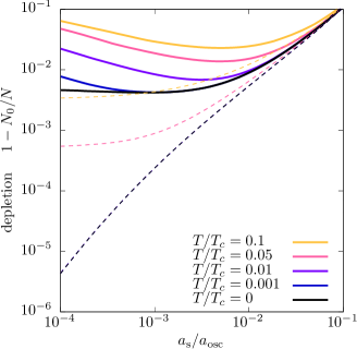
Figure 1: (Color Online) Depletions of the condensate $1-N_{0}/N$ as a function of ${a_{\mathrm{s}}}/{a_{\mathrm{osc}}}$ (solid lines) and the same results with the Bogoliubov approximation, where both $\expectationvalue*{\hat{Q}^{2}}$ and $\expectationvalue*{\hat{P}^{2}}$ are set to zero (dashed lines). The dashed lines with $T/T_{c}=0.01$ and $0.001$ are closely overlapping to that with $T/T_{c}=0$.

The result of the depletion is illustrated in Fig. 1. The fact is that while the zero mode contribution, absent in the Bogoliubov approximation, is negligible for the stronger interaction, it becomes noticeable for the weaker interaction. The ${a_{\mathrm{s}}}/{a_{\mathrm{osc}}}$-dependence in the weakly interacting case is enhanced as the temperature increases, and then the depletion, or the reduction of $N_{0}$, is attributed mainly to quantum and thermal fluctuations of the zero mode.

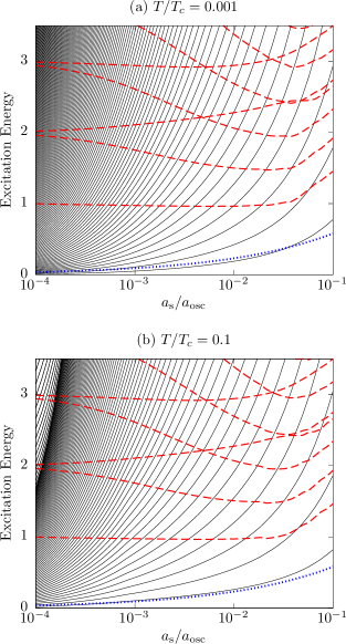
Figure 2: (Color Online) Excitation energy as a function of ${a_{\mathrm{s}}}/{a_{\mathrm{osc}}}$ in unit of $\omega$. The dashed red line denotes the BdG excitation $\omega_{\bm{\lambda}}$, and the solid black line denotes that of zero mode $E_{\nu}-E_{0}$ ($\nu=1,2,\cdots)$. The dotted blue line indicates the variational result for the first zero mode excitation $\Delta\mathcal{E}$.

In Fig. 2, we show the spectra of the zero mode and BdG excitations for lower and higher temperatures as a function of the interaction strength, $a_{\mathrm{s}}/a_{\mathrm{osc}}$, which give us an account of the behaviors in Fig. 1. The spectra depend only slightly on temperature. The excitation energy of the zero mode increases conspicuously as the interaction becomes stronger, whereas that of the BdG mode is rather robust. Explicitly, the first excited energy of the zero mode $E_{1}-E_{0}$ is approximately $0.02\omega$ for ${a_{\mathrm{s}}}/{a_{\mathrm{osc}}}=10^{-4}$, and increases to $0.8\omega$ for ${a_{\mathrm{s}}}/{a_{\mathrm{osc}}}=10^{-1}$, which is comparable with the BdG excitation energy. The theoretical estimations (39) and (42), predicting that energy levels vary as $(a_{\mathrm{s}}/a_{\mathrm{osc}})^{2/5}$, roughly trace the behaviors in Fig. 2. Considering that a typical thermal energy $k_{\mathrm{B}}T$ varies between $0.001\omega$ and $\omega$ over the temperature range under consideration, we see that the BdG mode is hardly excited thermally. The thermal excitation of the zero mode is also inhibited for stronger interaction, such as for $a_{\mathrm{s}}/a_{\mathrm{osc}}=10^{-1}$. However, as ${a_{\mathrm{s}}}/{a_{\mathrm{osc}}}$ is smaller, the spacing of the zero mode excitation energy becomes narrower, and much narrower than $k_{\mathrm{B}}T\sim\omega$ for $T/T_{c}=0.1$ and is comparable with $k_{\mathrm{B}}T\sim 0.01\omega$ for $T/T_{c}=0.001$. As a result, the thermal excitations of the zero mode are inconsiderable for $T/T_{c}=0.001$, but substantial for $T/T_{c}=0.1$.

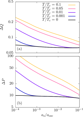
Figure 3: (Color Online) Interaction dependences of the phase fluctuation $\Delta Q$ and number fluctuation $\Delta P$.

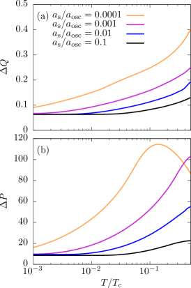
Figure 4: (Color Online) Temperature dependences of the phase fluctuation $\Delta Q$ and number fluctuation $\Delta P$.

It is important to argue about the fluctuations of the phase $\Delta Q$ and the number of condensate atoms $\Delta P$ from the dependences of the zero mode excitation spectrum on temperature and interaction strength. Their numerical results are shown in Figs. 3 and 4. Both of the fluctuations are almost constant irrespective of the interaction strength at zero temperature, which is in good agreement with the analytical results in Ref. [12], and increase with increasing temperature. This is more apparent in a weakly interacting case, where the spacing of the zero mode excitation energy is narrow and the thermal excitation is active. The irregular temperature dependence of $\Delta P$ in the weakly interacting case ($a_{\mathrm{s}}/a_{\mathrm{osc}}=10^{-4}$) is seen in Fig. 4, and it does not increase monotonically, but decreases beyond $T/T_{c}=0.1$. This is because a smaller number of condensate atoms $N_{0}$ result in a smaller fluctuation $\Delta P$.

4 Thermodynamical quantity and partition function

We consider the influences of the zero mode excitations on thermodynamical quantities that are derived from the partition function. As an example, the specific heat is calculated numerically.

4.1 Partition function

The partition function in our approximation is given in a factorized form,

$$Z =\mathrm{Tr}\,[\exp\,(-\beta\hat{H}_{u})]=Z_{\mathrm{z}}Z_{\mathrm{ex}}$$

$$Z_{\mathrm{z}} =\mathrm{Tr}_{\mathrm{z}}\,[\exp\,(-\beta\hat{H}_{u,\mathrm{z}})]=\sum_{\nu}\,e^{-\beta E_{\nu}}$$

$$Z_{\mathrm{ex}} =\mathrm{Tr}_{\mathrm{ex}}\,[\exp\,(-\beta\hat{H}_{u,\mathrm{ex}})]=\prod_{\bm{\lambda}}\,\frac{e^{\beta\omega_{\bm{\lambda}}}}{e^{\beta\omega_{\bm{\lambda}}}-1}\,,$$ (43)

where $\mathrm{Tr}_{\mathrm{z}}$ and $\mathrm{Tr}_{\mathrm{ex}}$ stand for traces over the zero mode subspace and Fock space of the Bogoliubov modes, respectively. Because $\ln Z=\ln Z_{\mathrm{z}}+\ln Z_{\mathrm{ex}}$, the thermodynamical quantities are given as sums of zero mode contributions and Bogoliubov ones. For example, the internal energy is

$$U =-\frac{\partial}{\partial\beta}\ln Z=-\frac{\partial}{\partial\beta}\ln Z_{\mathrm{z}}-\frac{\partial}{\partial\beta}\ln Z_{\mathrm{ex}}$$

$$=\frac{\sum_{\nu}\,E_{\nu}\,e^{-\beta E_{\nu}}}{\sum_{\nu}\,e^{-\beta E_{\nu}}}+\sum_{\bm{\lambda}}\,\frac{\omega_{\bm{\lambda}}}{e^{\beta\omega_{\bm{\lambda}}}-1}\,.$$ (44)

4.2 Specific heat

The specific heat is derived from the above $Z$,

$$C =\frac{1}{k_{\mathrm{B}}T^{2}}\frac{\partial^{2}}{\partial\beta^{2}}\ln Z=C_{\mathrm{z}}+C_{\mathrm{ex}}$$

$$C_{\mathrm{z}} =\frac{1}{k_{\mathrm{B}}T^{2}}\left\{\frac{\sum_{\nu}\,E^{2}_{\nu}\,e^{-\beta E_{\nu}}}{\sum_{\nu}\,e^{-\beta E_{\nu}}}-\left(\frac{\sum_{\nu}\,E_{\nu}\,e^{-\beta E_{\nu}}}{\sum_{\nu}\,e^{-\beta E_{\nu}}}\right)^{2}\right\}$$

$$C_{\mathrm{ex}} =\frac{1}{k_{\mathrm{B}}T^{2}}\sum_{\bm{\lambda}}\,\frac{\omega_{\bm{\lambda}}^{2}\,e^{\beta\omega_{\bm{\lambda}}}}{(e^{\beta\omega_{\bm{\lambda}}}-1)^{2}}\,.$$ (45)

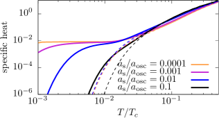
Figure 5: (Color Online) Temperature dependences of the specific heat beyond the Bogoliubov approximation (solid lines) and the one in the Bogoliubov approximation (dashed lines).

The numerical result of the specific heat $C$ from Eq. (45) is shown in Fig. 5. For comparison, we recall that the specific heat for an ideal gas trapped by a harmonic potential behaves as $(T/T_{c})^{3}$ under the approximation that a sum over the spectrum may be replaced with an integral [23]. The result of the specific heat in the Bogoliubov approximation is also depicted in Fig. 5. Both the plots, in and beyond the Bogoliubov approximation, are roughly fitted by a line of the ideal gas approximation $(T/T_{c})^{3}$ above $T/T_{c}\sim 5\times 10^{-2}$. Below the temperature, the plot in the Bogoliubov approximation (dashed line in Fig. 5) decreases rapidly due to suppression of the thermal excitation of the BdG mode, and the repulsive interaction increases the energy level of the BdG mode as in Fig. 2 and reinforces the suppression. A notable result in our approach is that the plot beyond the Bogoliubov approximation (solid line in Fig. 5) gets a plateau for weaker interaction strength and at lower temperature instead of falling down immediately. This is true as long as the spacing of the zero mode excitation energy (see Fig. 2) is smaller than a typical thermal energy $k_{\mathrm{B}}T$. In other words, an external energy is distributed to the densely populated excitation energy levels of the zero mode, thus the specific heat is kept constant for a while. When the temperature increases, the effects of the BdG modes with many degrees of freedom dominates those of the zero mode that has a single degree of freedom.

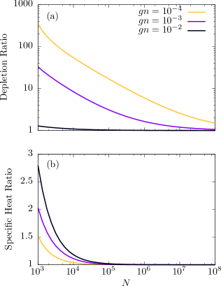
Figure 6: (Color Online) Ratios of the depletion and specific heat in the homogeneous IZMF to those in the Bogoliubov approximation as a function of $N$ at $T/T_{c}=0.01$. The quantity $gn$ is set dimensionless here.

4.3 Comparison between IZMF and Bogoliubov approximation for homogeneous system

A large $N$ limit of the IZMF is an interesting aspect to be explored. The numerical calculation for the inhomogeneous system trapped by a confining potential and with large $N$ is a heavy load, thus we study a homogeneous system instead, described by the Hamiltonian (1) without the trapping harmonic potential, for a large $N$ . It is straightforward to develop the IZMF for the homogeneous system. When the zero mode sector is dropped, we have the well-known formulation of a homogeneous system in the Bogoliubov approximation.

We assume a system with finite $N$ and $V$ and apply the homogeneous IZMF as above to it and increase $N$ at $T/T_{c}=0.01$, keeping the density $n=N/V$ constant. The ratios of the depletion and specific heat in the homogeneous IZMF to those in the Bogoliubov approximation versus $N$ are shown in Fig. 6. It is confirmed that both the ratios converge to unity at a large $N$ limit, which implies that the IZMF and the ordinary formulation of the Bogoliubov approximation cannot be distinguished from each other in the thermodynamical limit. On the other hand, the ratios are rather large for small $N$ and the zero mode effects are clear then.

5 Summary

In this paper, the unperturbed formulation for an inhomogeneous condensate system at finite temperature beyond the Bogoliubov approximation, called the IZMF, is given. While the zero mode operators are being treated properly, the infrared divergence, inevitable in the conventional formulation, is regularized by including the zero mode interaction into the unperturbed Hamiltonian. Then, a unique and stationary density matrix is defined, which allows us to calculate observables at thermal equilibrium.

The whole energy spectrum of the inhomogeneous condensate system consists of two parts, the BdG discrete spectrum, also existing in the Bogoliubov approximation, and the zero mode discrete spectrum equivalent to a one-dimensional quantum mechanical bound system. The level spacings of the two spectra and a typical thermal energy $k_{\mathrm{B}}T$ are key parameters. For realistic experiments in confined cold atomic gas, the spacing of the zero mode energy varies from being comparable with that of the BdG mode in stronger interaction to being much smaller in weaker interaction. The zero mode excitation in weaker interaction has distinctive effects on the depletion and specific heat at the unperturbed level. Although we cannot tell much about the condensate fraction and critical temperature shift[26, 27] that were observed at higher temperuture and for stronger interaction, our results at the unpertubed level does not contradict with the experimentally observed negative shift of the critical temperature.

Observing the zero mode operators $\hat{Q}$ and $\hat{P}$ that are canonical variables, we have noticed that their uncertainty does not reach its minimum value even in very weak interactions because of the very low excitation energies of the zero mode. The spread of the uncertainty may be observed, e.g. directly from the visibility of an interference fringe, or indirectly from an enhancement in the specific heat, if a condensate formation of very weakly interacting atoms in thermal equilibrium is achieved despite experimental difficulties.

It is an interesting question how the IZMF for the inhomogeneous system and the widely-used formulation in the Bogoliubov approximation for the homogeneous system are related to each other. As discussed in Subsect. 4.3, the quantities in the IZMF approach the calculated values of the Bogoliubov approximation in a large $N$ limit or in the thermodynamical limit for a homogeneous system. This verifies the validity of the Bogoliubov approximation for homogeneous systems, but we stress here that the Bogoliubov approximation is not valid for inhomogeneous systems, such as trapped cold atomic gas.

Although this study is restricted to the quantities over the unperturbed density matrix, it is possible to perform a systematic calculation of higher order perturbation in future. For this, we emphasize that our unperturbed formulation for a finite-size system satifsies all the requirements of quantum field theory, including the canonical commutation relations, and is free from the infrared divergence.

References

References

- [1] M. H. Anderson, J. R. Ensher, M. R. Matthews, C. E. Wieman, E. A. Cornell, Observation of Bose–Einstein condensation in a dilute atomic vapor, Science 269 (5221) (1995) 198–201. doi:10.1126/science.269.5221.198.
-
[2]
K. B. Davis, M. O. Mewes, M. R. Andrews, N. J. van Druten, D. S. Durfee, D. M.
Kurn, W. Ketterle,
Bose–Einstein
condensation in a gas of sodium atoms, Phys. Rev. Lett. 75 (1995)
3969–3973.
doi:10.1103/PhysRevLett.75.3969.
URL http://link.aps.org/doi/10.1103/PhysRevLett.75.3969 -
[3]
C. C. Bradley, C. A. Sackett, J. J. Tollett, R. G. Hulet,
Evidence of
Bose–Einstein condensation in an atomic gas with attractive
interactions, Phys. Rev. Lett. 75 (1995) 1687–1690.
doi:10.1103/PhysRevLett.75.1687.
URL http://link.aps.org/doi/10.1103/PhysRevLett.75.1687 -
[4]
J. Goldstone, Field theories with
« superconductor » solutions, Nuovo Cimento 19 (1) (1961) 154–164.
doi:10.1007/BF02812722.
URL http://dx.doi.org/10.1007/BF02812722 -
[5]
Y. Nambu, G. Jona-Lasinio,
Dynamical model of
elementary particles based on an analogy with superconductivity. I, Phys.
Rev. 122 (1961) 345–358.
doi:10.1103/PhysRev.122.345.
URL http://link.aps.org/doi/10.1103/PhysRev.122.345 - [6] N. N. Bogoliubov, J. Phys. (Moscow) 11 (1947) 32.
- [7] P. G. de Gennes, Superconductivity of Metals and Alloys, Benjamin, 1966.
- [8] A. L. Fetter, Ann. Phys. 70 (1972) 67.
-
[9]
M. Lewenstein, L. You,
Quantum phase
diffusion of a Bose–Einstein condensate, Phys. Rev. Lett. 77 (1996)
3489–3493.
doi:10.1103/PhysRevLett.77.3489.
URL http://link.aps.org/doi/10.1103/PhysRevLett.77.3489 -
[10]
H. Matsumoto, S. Sakamoto,
Quantum phase
coordinate as a zero-mode in Bose–Einstein condensed states, Prog.
Theor. Phys. 107 (4) (2002) 679–688.
doi:10.1143/PTP.107.679.
URL http://ptp.oxfordjournals.org/content/107/4/679.abstract -
[11]
M. Mine, M. Okumura, Y. Yamanaka,
Relation
between generalized Bogoliubov and Bogoliubov–de Gennes approaches
including Nambu–Goldstone mode, J. Math. Phys. 46 (4) (2005) 042307.
doi:http://dx.doi.org/10.1063/1.1865322.
URL http://scitation.aip.org/content/aip/journal/jmp/46/4/10.1063/1.1865322 -
[12]
Y. Nakamura, J. Takahashi, Y. Yamanaka,
Formulation for the
zero mode of a Bose–Einstein condensate beyond the Bogoliubov
approximation, Phys. Rev. A 89 (2014) 013613.
doi:10.1103/PhysRevA.89.013613.
URL http://link.aps.org/doi/10.1103/PhysRevA.89.013613 -
[13]
Y. Nakamura, J. Takahashi, Y. Yamanaka, S. Ohkubo,
Effective field
theory of Bose–Einstein condensation of clusters and
Nambu–Goldstone–Higgs states in 12C, Phys. Rev. C 94 (2016)
014314.
doi:10.1103/PhysRevC.94.014314.
URL http://link.aps.org/doi/10.1103/PhysRevC.94.014314 -
[14]
W. Krauth, Quantum
Monte Carlo calculations for a large number of Bosons in a harmonic
trap, Phys. Rev. Lett. 77 (1996) 3695–3699.
doi:10.1103/PhysRevLett.77.3695.
URL http://link.aps.org/doi/10.1103/PhysRevLett.77.3695 -
[15]
M. Holzmann, W. Krauth, M. Naraschewski,
Precision Monte
Carlo test of the Hartree–Fock approximation for a trapped Bose
gas, Phys. Rev. A 59 (1999) 2956–2961.
doi:10.1103/PhysRevA.59.2956.
URL http://link.aps.org/doi/10.1103/PhysRevA.59.2956 -
[16]
J. L. DuBois, H. R. Glyde,
Natural orbitals
and Bose–Einstein condensates in traps: A diffusion Monte Carlo
analysis, Phys. Rev. A 68 (2003) 033602.
doi:10.1103/PhysRevA.68.033602.
URL http://link.aps.org/doi/10.1103/PhysRevA.68.033602 -
[17]
A. Griffin, Conserving
and gapless approximations for an inhomogeneous Bose gas at finite
temperatures, Phys. Rev. B 53 (1996) 9341–9347.
doi:10.1103/PhysRevB.53.9341.
URL http://link.aps.org/doi/10.1103/PhysRevB.53.9341 - [18] A. Griffin, T. Nikuni, E. Zaremba, Bose–Condensed Gases at Finite Temperatures, Cambride University Press, 2009.
- [19] T. Kita, Conserving gapless mean–field theory for Bose–Einstein condensates, J. Phys. Soc. Jpn. 74 (7) (2005) 1891–1894. doi:10.1143/JPSJ.74.1891.
- [20] T. Kita, Conserving gapless mean–field theory for weakly interacting Bose gases, J. Phys. Soc. Jpn. 75 (4) (2006) 044603. doi:10.1143/JPSJ.75.044603.
-
[21]
K. Kobayashi, Y. Nakamura, M. Mine, Y. Yamanaka,
Analytical
study of the splitting process of a multiply-quantized vortex in a
Bose–Einstein condensate and collaboration of the zero and complex
modes, Ann. Phys. 324 (11) (2009) 2359.
doi:http://dx.doi.org/10.1016/j.aop.2009.07.004.
URL http://www.sciencedirect.com/science/article/pii/S0003491609001262 -
[22]
A. Mann, M. Revzen, H. Umezawa, Y. Yamanaka,
Relation
between quantum and thermal fluctuations, Phys. Lett. A 140 (9) (1989) 475.
doi:10.1016/0375-9601(89)90125-4.
URL http://www.sciencedirect.com/science/article/pii/0375960189901254 - [23] C. J. Pethick, H. Smith, Bose–Einstein Condensation in Dilute Gases, Cambridge University Press, 2008.
-
[24]
J. R. Ensher, D. S. Jin, M. R. Matthews, C. E. Wieman, E. A. Cornell,
Bose–Einstein
condensation in a dilute gas: Measurement of energy and ground-state
occupation, Phys. Rev. Lett. 77 (1996) 4984–4987.
doi:10.1103/PhysRevLett.77.4984.
URL http://link.aps.org/doi/10.1103/PhysRevLett.77.4984 -
[25]
S. Bhattacharyya, T. K. Das, B. Chakrabarti,
Effects of
interaction on thermodynamics of a repulsive Bose–Einstein condensate,
Phys. Rev. A 88 (2013) 053614.
doi:10.1103/PhysRevA.88.053614.
URL http://link.aps.org/doi/10.1103/PhysRevA.88.053614 -
[26]
F. Gerbier, J. H. Thywissen, S. Richard, M. Hugbart, P. Bouyer, A. Aspect,
Critical
temperature of a trapped, weakly interacting Bose gas, Phys. Rev. Lett. 92
(2004) 030405.
doi:10.1103/PhysRevLett.92.030405.
URL http://link.aps.org/doi/10.1103/PhysRevLett.92.030405 -
[27]
R. P. Smith, R. L. D. Campbell, N. Tammuz, Z. Hadzibabic,
Effects of
interactions on the critical temperature of a trapped Bose gas, Phys. Rev.
Lett. 106 (2011) 250403.
doi:10.1103/PhysRevLett.106.250403.
URL http://link.aps.org/doi/10.1103/PhysRevLett.106.250403