Random selection of factors preserves the correlation structure in a linear factor model to a high degree

Abstract

In a very high-dimensional vector space, two randomly-chosen vectors are almost orthogonal with high probability. Starting from this observation, we develop a statistical factor model, the random factor model, in which factors are chosen at random based on the random projection method. Randomness of factors has the consequence that covariance matrix is well preserved in a linear factor representation. It also enables derivation of probabilistic bounds for the accuracy of the random factor representation of time-series, their cross-correlations and covariances. As an application, we analyze reproduction of time-series and their cross-correlation coefficients in the well-diversified Russell 3,000 equity index.

1 Introduction

1.1 Vectors in a high-dimensional space

Any two randomly-selected vectors in a high-dimensional vector space are likely almost orthogonal with respect to each other (Hecht-Nielsen, 1994; Kaski, 1998). This observation has relevance to time-series analysis, since a long time-series corresponds to a vector in a high-dimensional vector space and orthogonality of vectors corresponds to uncorrelatedness of time-series. Hence, time-series corresponding to the two randomly-selected vectors are almost uncorrelated.

When the length of the time-series increases, or equivalently, dimension of the vector space increases, the probability that two randomly-selected time-series are uncorrelated increases (Hecht-Nielsen, 1994). If we select a set of, say, $n$ vectors randomly, these vectors are approximately orthogonal to each other if the dimension of the space is sufficiently high. Then, high-dimensionality of the data may in some cases even be an asset: in a high-dimensional space, almost any set of random vectors yields an almost uncorrelated set of factor time-series that can be used as a basis for a linear factor model.

1.2 Factor models

Factor models are extensively used in financial applications to model asset returns (see, e.g., Campbell et al. (1997)) and to decompose them to loadings of risk factors. The two main types of factor models are fundamental factor models and statistical factor models. In a fundamental factor model, the aim is to find observable asset characteristics, e.g., financial ratios and macro-economic variables, capable of explaining the behavior of the market stock prices, that are often extrinsic to the asset time-series.

The explanatory fundamental and economic variables can be highly correlated with each other, which may cause, e.g., multi-collinearity in a fundamental factor model. Returns predicted by a fundamental factor model may then be more correlated than the observed returns, which is the main reason for the inclusion of specific risk components in a factor model.

Statistical factor models are a commonly-used alternative for fundamental factor models. In a statistical factor model, factors are extracted from asset returns. The principal component analysis (PCA; see, e.g., Alexander (2001)) is an example of a statistical technique for finding factors from asset time-series.

PCA works well when the analyzed time-series are highly correlated, which may indicate the presence of a common driver. Applications of PCA include models of interest rate term structure, credit spreads, futures, and volatility forwards. In PCA, several principal components often have an intuitive financial interpretation. In ordered highly-correlated systems, the first principal component captures an almost parallel shift in all variables and is generally labeled the common trend component. The second principal component captures an almost linear tilt in the variables, while the higher order principal components capture changes that are quadratic, cubic and so forth (see, e.g., Alexander (2009)). In the equity markets, the higher order principal components may often, but certainly not always, be interpreted as market movements caused by different investment style tilts.

Stock and Watson (2002) show that principal components found using PCA provide consistent estimators of the true latent factors in the limit of both time and cross-sectional size go to infinity. They extend consistent estimation of the classical factor model with non-correlated errors to approximate factor models with cross-correlated and sectionally-correlated error terms.

Classical factor models include only a handful of factors. The best-known factor model in the literature is likely the Capital Asset Pricing Model (CAPM), which assumes that a single risk factor, the market, drives returns in a portfolio of assets (Sharpe, 1964). A number of factor models have extended this view (see, e.g., Ross (1976); Fama and French (1993)). Recent increase in computational power has enabled development of models with a large set of factors. Today, factor models are popular in market risk modeling, e.g., the Barra models (Grinold and Kahn, 2000) depend on hand-picked market factors to explain behavior of the analyzed financial instruments.

Boivin and Ng (2006) demonstrate that there are situations in which the use of a larger number of time-series may actually result a worse factor estimate than a smaller number of time-series. A significant amount of recent literature has been devoted to address the issue of consistent estimation under conditions where the number of time-series is large compared to the length of time-series (e.g., Bun et al. (2017); Ledoit and Wolf (2012)).

1.3 Choice of factors

The choice of factors clearly influences the ability of a factor model to explain investment risk of a portfolio, in particular when the factor model consists of only a few carefully-chosen factors. When the number of factors is large compared to the number of time-series analyzed, it may not much matter which factors are chosen as long as the factors span a sufficiently large sample space. Even then, relative importance of factors is often of interest in risk management. However, it is not clear how well an arbitrary set of factors would enable analysis - or at least description - of the risk. This is the issue that we analyze in this study: take a random set of factors and see whether it enables reproduction of the data and its interdependencies.

A good starting point for developing a random factor model is the random projection method (see, e.g, Bingham and Mannila (2001); Vempala (2005)) that consists of a projection of data to a lower-dimensional space by a random matrix. The random projection method has been used, e.g., to reduce the complexity of the data for classification purposes (Kohonen et al. (2000)), for structure-preserving perturbation of confidential data in scientific applications (Liu et al., 2006), for data compression (Bingham and Mannila, 2001), for compression of images (Amador, 2007), and in the design of approximation algorithms (Blum, 2006). The random projection allows one to reduce dimensionality of the investigated problem, often substantially, while preserving the structure of the problem.

From the econometric point of view, a random projection can be viewed as a projection of time-series to a collection of almost non-autocorrelated factors that are also expected to be non-cross-correlated, as will be seen in Section 2.

1.4 Correlation structure and random matrices

Analysis of risk in an investment portfolio requires that risks of individual instruments are combined into the risk of the portfolio. This can be accomplished using dependence structures, e.g., correlation matrix. It is no coincidence that dependence structures of financial time-series are central in modern investment theory (e.g., Markowitz (1952)).

The recent explosion of available data has brought new issues with time-series analysis (e.g., Bun et al. (2017)). To get around these issues, new methods of analysis are needed. One such tool is the random matrix theory (e.g., Edelman and Rao (2005)). It is typical in the random matrix theory that things get less complex when dimension of the problem increases.

A number of studies have applied random matrix theory to analyze correlations. The Tracy-Widom distribution (Tracy and Widom, 1996) gives distribution of the largest normalized eigenvalue in Gaussian Orthogonal Ensemble. There are also versions of the theorem for other random matrix ensembles (Tracy and Widom, 1994, 1996). The Tracy-Widom distribution is an example of universality found in the random matrix theory. Another important example of universality in random matrix theory is the Marchenko-Pastur law (Marchenko and Pastur, 1967), which describes the asymptotic distribution of eigenvalues of a covariance matrix.

Laloux et al. (1999) argue that most of the eigenvalue spectrum of correlation matrix for the Standard & Poor’s 500 Index (S&P 500) equities can be described as a product of noise, only about 20 eigenvalues of 500 total are informative. In more detail, Laloux et al. (1999) demonstrated that the bulk of the power spectrum of the S&P 500 returns is indistinguishable from that produced by Gaussian Orthogonal Ensemble, in which the asymptotic eigenvalue distribution is given by the Marchenko-Pastur law (Marchenko and Pastur, 1967). Since Gaussian Orthogonal Ensemble consists of random matrices, the bulk of power spectrum can be explained as a product of noise.

The informative eigenvalues may correspond to the market movements and sectors, but most of the eigenvalue spectrum does not correspond to linear factors. This suggests that noise has a significant role in the description of dependence structures in financial data.

Plerou et al. (1999) show that the most eigenvalues in the spectrum of the cross-correlation matrix of stock price changes agree surprisingly well with universal predictions of random matrix theory. Malevergne and Sornette (2004) construct a model with a spectrum that exhibits the features found in S&P 500 spectrum: a few large eigenvalues and a bulk part. Malevergne and Sornette (2004) also point out the chicken-and-egg problem associated with factors: factors exist because stocks are correlated; stocks are correlated because of a common factor impacting them. They argue that the apparent presence of factors is a consequence of the collective, bottom-up effect of the underlying time-series.

Ledoit and Wolf (2004) show that a naive use of the sample covariance matrix has drawbacks, and that shrinkage of the sample covariance matrix toward a structured or a constant matrix reduces extremal estimation errors. In a subsequent work, Ledoit and Wolf (2012) use Marchenko-Pastur law to improve the results further.

Bun et al. (2017) give a concise review of the random matrix theory and then move on to show how it can be used to alleviate the issues of ”Big data”. In particular, they describe the issues of correlation matrix estimation when there are more time-series than data points in each time-series. They also suggest remedies based on the the random matrix theory that can be used to improve empirical estimates of correlation matrices.

Given the above examples, it is clear that the random matrix theory has already contributed to the analysis of financial time-series. We make use of random matrices to develop a factor model and to analyze the properties of correlation matrix preservation in a generic linear factor model.

1.5 This study

It is largely an open question whether and how well randomly-chosen factors can be used to describe a large data set. This is the issue we approach in this study. For this purpose we develop a factor model based on randomly-chosen factor time-series, the random factor model. We show that randomness of factors has certain desirable properties, such as well-defined probabilistic limits on the accuracy of the factor representation. In addition, randomly-chosen factors are almost orthogonal with high probability, and with a proper normalization, they are expected to be orthonormal. We also show how the random factor model converges toward the modeled data when the number of factors increases, and that a random factor model preserves pair-wise correlations well with high probability.

The article is structured as follows. In Section 2, we develop the random factor model based on the random projection method and derive theoretical results describing the model (more details can be found from Appendix A). For example, we show that randomness of factors enables derivation of theoretical results on the accuracy of the model.

As an application of the random factor model, Section 3 provides an analysis of the correlation matrix of Russell 3,000 equity index using the factor models described in Section 2. We analyze the ability of random factor models to reproduce equity log-return time-series and their correlations and covariances. The reproduction of data in a random factor model is compared with a reproduction obtained using principal component analysis both at the individual time-series level and at the dependence structure level.

In Section 4, we compare different random factor models and show that the results, or rather their accuracy, are quite universal. In Section 5, we discuss the results and their possible implications.

In Appendix A, we prove a version of the Johnson-Lindenstrauss-like theorem appropriate for the random factor model. It gives probabilistic bounds on the accuracy of the correlation and covariance preservation in a random factor model.

2 Random factor model

2.1 Notations

Let $d$ observations of time-series $Z:{\mathbb{N}}\to{\mathbb{R}}$ be viewed as a vector in $d$-dimensional space ${\mathbb{R}}^{d}$, where each observation of the time-series corresponds to one coordinate of the vector. The set of $N$ such time-series can be packed into matrix $X\in{\mathbb{R}}^{d\times N}$, in which observations are in columns. We assume that the time-series data has been preprocessed, so that each time-series is averaged to zero, that is, $\sum_{m}X_{mb}=0$ for each $b=1,...,N$. We employ sample statistics in this study. Definitions for mean $\mu$, variance $\sigma^{2}$ and covariance $C$ are

$$\mu_{x}={\frac{1}{d}}\sum_{m=1}^{d}x_{m},\qquad C_{x,y}={\frac{1}{d-1}}\sum_{m=1}^{d}(x_{m}-\mu_{x})(y_{m}-\mu_{y}),\qquad\sigma^{2}_{x}=C_{x,x},\qquad$$ (1)

where $x,y\in{\mathbb{R}}^{d}$. The central parameters used in this study are summarized in Table 1.

Parameter	Description
$d$	Number of data points in each time-series
$N$	Number of time-series, e.g., equities
$k$	Number of factors

Table 1: The central parameters used.

2.2 Linear factor models

A linear factor model describes the target data set as a loading-weighted sum of factors (e.g., McNeil et al. (2015)). Let $F=[F_{1}\,F_{2}\,...\,F_{k}]\in{\mathbb{R}}^{d\times k}$ contain $d$ observations of the factors $j=1,2,\ldots,k$, $F_{j}\in{\mathbb{R}}^{d\times 1}$. Then time-series $X_{b}\in{\mathbb{R}}^{d\times 1}$, where $X_{b}$ is $b$:th column of matrix $X$, $b=1,...,N$, can be represented as a sum of products of factor loadings $L_{bj}\in{\mathbb{R}}$ and factors $F_{j}$, that is,

$$X_{b}=\sum_{j=1}^{k}L_{bj}F_{j}+\epsilon_{b},$$ (2)

where $\epsilon_{b}$ is an idiosyncratic risk component. Since we collect the observations into columns of $X$ and $F$, the formula (2) is written in a matrix form as $X=FL^{T}+\epsilon$.

Factors in $F$ may or may not be directly observable in the market data. For observed factor time-series, it suffices to project the data to factors to get loadings. For unobserved factor time-series, some method such as PCA or some other optimization-like method is required to find the factors and their loadings.

2.3 Random projection

Random factors are here chosen using the random projection method. The key idea of random projection is based on the Johnson-Lindenstrauss lemma (Johnson and Lindenstrauss, 1984; Bingham and Mannila, 2001): if points in a high-dimensional space are projected onto a randomly selected subspace of suitably high dimension, then the distances between the points are approximately preserved. A suitably high-dimensional subspace has dimension proportional to $\log(N)/\varepsilon$, where $N$ is the number of time-series and $\varepsilon$ the desired accuracy (Dasgupta and Gupta, 2003).

Random projection $Q:{\mathbb{R}}^{d\times N}\to{\mathbb{R}}^{k\times N}$ of matrix $D\in{\mathbb{R}}^{d\times N}$ is a mapping defined by $Q(D)=BD$, where $k,d,N\in{\mathbb{N}}$. Here matrix $B$ is realization $B(\omega)$ of a random variable-valued $k\times d$ matrix.

A large variety of probability distributions can be used to construct projection matrix $B$ (more on this in Section 3.3). The most obvious choice is to assume that matrix $B$ is taken from the matrix-variate normal distribution with independent entries, that is, from $N_{k\times d}(0,1_{k}\times 1_{d})$ (Gupta and Nagar, 1999). Then each element is $N(0,1)$-distributed and independent of other elements.

2.4 Random factor model

2.4.1 Definition and properties

We define the random factor model (RFM) for data set $X\in{\mathbb{R}}^{d\times N}$ via a projection $P:{\mathbb{R}}^{d\times N}\to{\mathbb{R}}^{d\times N}$,

$$PX=aB^{T}BX,$$ (3)

where $B\in N_{k\times d}(0,1_{k}\times 1_{d})$ is a $k\times d$-dimensional random variable, elements of which are independent and normally distributed, and $a>0$ is a normalization constant. Mapping (3) can be interpreted as a linear factor model by setting

$$L=\frac{a}{a^{\prime}}X^{T}B^{T},\\ \quad F=a^{\prime}B^{T}\,,$$ (4)

where $a^{\prime}>0$ is a constant related to factor normalization, as discussed in Section 2.4.3. Then $F\in{\mathbb{R}}^{d\times k}$ behaves as a matrix of $k$ $d$-dimensional factor time-series. It is worth stressing that matrix $F$ consists of random time-series that in no way depend on the data. $L\in{\mathbb{R}}^{N\times k}$ is a matrix of $k$ factor loadings for the $N$ time-series.

Projection $P$ can be factored as

$$PX=FL^{T}.$$ (5)

Defining $\epsilon^{*}=X-PX$ yields an approximate factorization

$$X=FL^{T}+\epsilon^{*}$$ (6)

for data matrix X. We will analyze equation (6), and in particular error term $\epsilon^{*}$, further in the following. Equation (6) shows that data matrix $X$ can be approximately decomposed to a product of two components.

As an aside, let us mention that we could equally well have considered a random projection in the equity direction instead of the above time-series direction. This can be accomplished using a matrix $Q=aR^{T}R$, where $a>0$ and $R\in{\mathbb{R}}^{k\times N}$ is a random matrix, and then considering $XQ$ as the projected matrix. This naturally leads to a factor model interpretation with a loading matrix $\frac{a}{a^{\prime}}R^{T}$ and a factor matrix $a^{\prime}XR^{T}$. In analogy to the earlier terminology, this model could be called random loading model. The properties proven later for the random projection $P$ then immediately carry over to the projection $Q$, one merely needs to replace “$d$” with “$N$” in all of the results.

However, from the point of view of the time series, the two projection methods $PX$ and $XQ$ could behave differently. For instance, if there are more pronounced correlations between different equities at a fixed time than between the same equity at two different times, then one would expect to need larger values of $k$ in the projection $XQ$ than in the projection $PX$ to reach the same level of accuracy in the approximation. It is also possible to apply both random projections simultaneously and study $PXQ$ instead of $PX$ or $XQ$. This double-sided projection would still have properties very similar to the one-sided projections, as long as the random matrices $B$ and $R$ are chosen independently of each other. Since the three alternatives are on a technical level very similar, we focus only on the choice $PX$ in the following.

As the next step, we need to find a suitable constant $a$ so that standard deviation, covariance and the expected value of the data are preserved, if possible. Under these conditions, $\epsilon^{*}$ should be close to zero. Different choices of $a$ yield slightly different properties for the RFM, but it turns out that we cannot satisfy all these requirements at the same time if we base matrix $B$ on the normal distribution.

Here we concentrate on preserving the covariance matrix $C_{x,y}$ in the projection. Then normalization constant $a>0$ must be such that expectation with respect to $N_{k\times d}(0,1_{k}\times 1_{d})$ is preserved, that is,

$$\mathbbm{E}[C_{Px,Py}]=C_{x,y}$$ (7)

for any zero-mean vectors $x,y\in{\mathbb{R}}^{d\times 1}$. It is worth stressing that the expectation in equation (7) is taken over random factor models, not over time-series $x$ and $y$. Theorem A.1 in the Appendix shows that this is possible but only if we choose $a=1/\sqrt{k(k+d)}$. Let $a$ have this value from this point on.

The expected covariance between time-series $x$ and $y$ is then preserved, regardless of the number of factors used. Since $\mathbbm{E}[\sigma^{2}_{Px}]=\mathbbm{E}[C_{Px,Px}]=C_{x,x}=\sigma^{2}_{x}$, our choice of $a$ also preserves time-series variance. This result shows that an RFM is expected to fulfill the consistency requirement of variance, that is, it shows that

$$\lim_{d\to\infty}\mathbbm{E}[\sigma^{2}_{Px,d}]=\lim_{d\to\infty}\sigma^{2}_{x,d}=\sigma^{2}_{x,\text{pop}},$$ (8)

where $\sigma^{2}_{x,\text{pop}}$ is the population variance and $\sigma^{2}_{x,d}$ is the sample variance in dimension $d$. An application of the Jensen’s inequality implies that $\mathbbm{E}[\sigma_{Px}]\leq\sigma_{x}$, that is, volatility is not over-estimated.

Representation (6) always preserves the average of a zero-mean vector $x\in{\mathbb{R}}^{d}$, that is, $\mathbbm{E}[\mu_{Px}]=0$. In contrast, the $m$:th observation $x_{m}$ of time-series $x$ has an expectation $\mathbbm{E}[(Px)_{m}]=\sqrt{k/(k+d)}x_{m}$ and a variance $(x_{m}^{2}+(d-1)\sigma_{x}^{2})/(d+k)$. For a small number of factors, mapping to $(Px)_{m}$ will on average underestimate the original value $x_{m}$ since $\sqrt{k/(k+d)}<1$. In the limit of large number of factors, $(Px)_{m}$ approaches $x_{m}$, since

$$\lim_{k\to\infty}\mathbbm{E}[(Px)_{m}]=\lim_{k\to\infty}\sqrt{k/(k+d)}x_{m}=x_{m}\,,$$ (9)

and the standard deviation of $(Px)_{m}$ is $O\left(\sqrt{d/(d+k)}\right)$ and thus goes to zero when $k\to\infty$. Hence, a RFM reproduces any vector $x\in{\mathbb{R}}^{n}$ component-by-component in the limit of large number of number of factors, for $k\gg d$. Thus $\epsilon$ of equation (6) approaches zero when the number of factors increases.

The RFM is expected to reproduce mean, variance and covariance of time-series $x$. Component-wisely, the random factor model is expected to converge to the observed component values in the limit of large number of factors.

2.4.2 Covariance preservation

Equation (7) does not state that each RFM always preserves the covariance matrix. Nevertheless, it is reasonable to assume that an RFM approximately preserves the covariance matrix. Next we will analyze how well an RFM will typically preserve the covariance matrix.

But first, it is worth recalling that Johnson-Lindenstrauss theorem (Johnson and Lindenstrauss, 1984; Dasgupta and Gupta, 2003; Matoušek, 2008) gives probabilistic bounds for the accuracy of distance preservation in the random projection. A number of versions of Johnson-Lindestrauss theorem have been proven, however, in all versions known to us, it is assumed that random variables have zero expectation.

Matrix $B^{T}B\in{\mathbb{R}}^{d\times d}$ is a singular Wishart matrix (also known as an anti-Wishart matrix), which has non-zero expectation, $d-k$ zero eigenvalues and $k$ non-zero eigenvalues. Since matrix $B^{T}B$ has non-zero expectation, it was not a priori clear if a Johnson-Lindenstrauss type theorem holds. Theorem A.1 proven in the Appendix fills this gap for the present type of anti-Wishart matrices, and it also contains a detailed derivation of the above expectation values for an arbitrary value of the scaling parameter $a$.

We have collected in Corollary A.2 the corresponding results for the choice which preserves the sample covariance matrices in expectation, for $a=1/\sqrt{k(k+d)}$. The precise control of fluctuations in the covariance estimates requires nontrivial combinatorial computations, given in the Appendix. As proven in Corollary A.2, for every $b>0$ and non-random vectors $u,v\in{\mathbb{R}}^{d}$, with $\mu_{u}=0=\mu_{v}$, we have

$$\mathbbm{P}\!\left[|C_{Pu,Pv}-C_{u,v}|\geq b\right]\leq\frac{8}{kb^{2}}\sigma_{u}^{2}\sigma_{v}^{2}\,.$$ (10)

Inequality (10) gives bounds on the accuracy of covariance preservation for an arbitrary random factor model. Here probability is taken with respect to an ensemble of random factor models.

Hence, if $\sigma_{u}^{2},\sigma_{v}^{2}\leq 1$, the probability that covariance of vectors $u$ and $v$ is preserved in a random factor model more accurately than bound $b$ is at least $1-8/(kb^{2})$, where $k$ is the number of factors. In general, we can set $b=\varepsilon\sigma_{u}\sigma_{v}$, with $\varepsilon>0$, and also conclude that the accuracy, relative to the sample variance scale $\sigma_{u}\sigma_{v}$, is at least $\varepsilon$ with a probability of at least $1-8/(k\varepsilon^{2})$. For the bound to be informative, it is necessary that $\varepsilon>k^{-1/2}$.

The error in the covariance estimate decreases at least inversely with the number of factors in almost any random factor model. Given a sufficient number of factors, covariance of any two time-series can be approximated with an arbitrarily high accuracy using an RFM. This and the fact that random factors are in no way fitted to the data suggest that the typical accuracy of an RFM depends mainly on the number of factors $k$.

Corollary A.2 also gives a bound on how accurately correlation between projected vectors is preserved. Correlation $\text{Corr}(u,v)$ coincides with covariance $C_{u,v}$ when $\sigma_{u}=\sigma_{v}=1$. Then inequality (10) gives a lower bound on how well $C_{Pu,Pv}$ approximates correlation between $u$ and $v$.

These results can be summarized as a statement about the projected matrix $PX$ as follows:

$$\mathbbm{P}\!\left[\frac{1}{\sigma_{X_{b}}\sigma_{X_{c}}}|C_{(PX)_{b},(PX)_{c}}-C_{X_{b},X_{c}}|<\varepsilon\right]\geq 1-\frac{8}{k\varepsilon^{2}}\,,$$ (11)

valid for any $b,c=1,2,\ldots,N$ and $\varepsilon>0$.

2.4.3 Almost orthogonality

Orthogonality is a desirable property of a factor set. An orthogonalization procedure can be used to obtain an orthogonal factor set, but orthogonalization is computationally expensive. Fortunately, orthogonalization is not a necessary step in the RFM.

Given any two random factors (as defined above), their inner product is expected to be orthogonal, that is,

$$\mathbbm{E}\left[\sum_{m=1}^{d}F_{mj}F_{mj^{\prime}}\right]=(a^{\prime})^{2}\sum_{m}\mathbbm{E}\left[B_{j^{\prime}m}B_{jm}\right]=(a^{\prime})^{2}d\delta_{j^{\prime},j}.$$ (12)

This shows that with the choice $a^{\prime}=1/\sqrt{d}$, the factors $F_{j^{\prime}}$ and $F_{j}$ are expected to be orthonormal as a consequence of the properties of normally distributed random variables.

Using Theorem A.1 we can also compute the variance of the inner product. This yields

$$\text{Var}\left[\sum_{m=1}^{d}F_{mj}F_{mj^{\prime}}\right]=\frac{1}{d}(\delta_{j^{\prime},j}+1)\leq\frac{2}{d}.$$ (13)

Higher cumulants approach zero even more rapidly, as can be seen by analyzing the cumulant generating function

$$\ln\mathbbm{E}\left[e^{\lambda\sum_{m=1}^{d}F_{mj}F_{mj^{\prime}}}\right]=\begin{cases}-\frac{d}{2}\ln(1-2\frac{\lambda}{d}),\quad\text{when $j=j^{\prime}$,}\\ -\frac{d}{2}\ln(1-\frac{\lambda^{2}}{d^{2}}),\quad\text{otherwise,}\end{cases}$$ (14)

and its series expansion in $\lambda$. When $j=j^{\prime}$, $n$th cumulant is of order $O(d^{1-n})$. When $j\neq j^{\prime}$, cumulants are of order $O(d^{1-n})$ for even $n$ and zero otherwise. Convergence to the Normal distribution in the limit of large $d$ then follows by the standard arguments (e.g., Billingsley (1995)).

Inner product matrix is approximately distributed as

$$\sum_{m=1}^{d}F_{mj}F_{mj^{\prime}}\sim\begin{cases}N(1,\sqrt{2/d}),\text{ when }j^{\prime}=j,\\ N(0,\sqrt{1/d}),\text{ otherwise}.\\ \end{cases}$$ (15)

When $d$ is large ($\gg 1000$), standard deviation is only a fraction of the expectation for diagonal elements. Fluctuations around zero are small for non-diagonal elements. The cumulant expansion shows that the factors are almost orthonormal even at a relatively low dimension.

In addition, the factors are on average orthogonal to the error term $\epsilon^{*}$: since $\epsilon^{*}$ is an even polynomial of $B$:s and $F_{j}$ is linear in them, we have $\mathbbm{E}\left[\sum_{m=1}^{d}F_{mj}\epsilon^{*}_{mb}\right]=0$ for all $j=1,2,\ldots,k$ and $b=1,2,\ldots,N$.

2.5 Principal component analysis

PCA is a well-known technique which uses a linear transformation to form a simplified data set retaining the characteristics of the original data set (see, e.g., Johnson et al. (2014)). In investment risk measurement, PCA is used to explain the covariance structure of a set of market variables through a few linear combinations of these variables. The general objectives of using PCA are to reduce the dimensions of covariance matrices and to find the main risk factors. The risk factors can then be used to analyze, e.g., the investment risk sources of a portfolio, or to predict how the value of the portfolio will develop.

Projection to principal components is most directly obtained using the singular value decomposition (Golub and Van Loan, 2012). Given data matrix $X\in{\mathbb{R}}^{d\times N}$, SVD decomposes it as $X=P_{L}DP_{R}^{T}$, where $P_{L}\in{\mathbb{R}}^{d\times d}$ is matrix of left singular vectors, $P_{R}\in{\mathbb{R}}^{N\times N}$ is matrix of right singular vectors, and $D\in{\mathbb{R}}^{d\times N}$ is the rectangular diagonal matrix of singular values. PCA-based factor representation of $X$ is given by $X=FL^{T}$, where $L=P_{R}\in{\mathbb{R}}^{N\times N}$ gives the factor loading matrix and $F=P_{L}D\in{\mathbb{R}}^{d\times N}$ defines the factors of the $N$ equities. When reducing the dimensions of the original dataset, the first $k$ principal components with the largest eigenvalues are chosen to represent the original dataset. This yields an approximation of the data matrix using a subset of factors. A $k$-factor approximation of matrix $X$ is given by $F^{(k)}(L^{(k)})^{T}$, where $L^{(k)}\in{\mathbb{R}}^{N\times k}$ contains the first $k$ factor loadings, $F^{(k)}\in{\mathbb{R}}^{d\times k}$ contains the components of the first $k$ factors from $P_{L}D$. It can be shown that in the mean-error sense, PCA gives the best linear $k$-factor approximation to matrix $X$ (e.g., Reris and Brooks (2005); Eckart and Young (1936)). Principal components correspond to directions along which there is most variation in the data. However, there are no guarantees that pair-wise distances are preserved in PCA.

PCA yields the relative importance of the most important risk sources (defined in factor matrix $F$) in an investment portfolio. The relative importance of risk factors is shown by the size of eigenvalues. The eigenvectors with highest eigenvalues correspond to the most important risk factors. Loadings then tell how much investment instruments depend on these factors.

Nevertheless, it should be stated that PCA aims to capture total variation, not correlations (Johnson et al., 2014).

2.6 Comparison of factor models

Despite appearance, the RFM and PCA share many features. In both models, the data can be represented as $FL^{T}$, where $L$ contains $k$ factor loadings and $F$ defines $k$ factor time-series with $d$ observations. In PCA, the most important eigenvectors are found by choosing the largest eigenvalues. No such ordering is available for random vectors. A random vector is essentially as good as the next random vector as a factor.

The RFM has an almost orthonormal factors, while PCA yields strictly orthonormal factors. After finding the factors, both the RFM and PCA project the data to these vectors. The ways in which the RFM and PCA end up with representations of the data matrix are quite different: in PCA, data is projected along principal components (factors) and only the desired set of these projections (loadings) are kept. In the RFM, the data is projected along the random factors. The main difference is in the way that factors are chosen.

PCA requires $O(d^{2}N)+O(d^{3})$ operations, while the RFM requires $O(kdN)$ operations, given the factor time-series. Since that the number of factors is typically significantly smaller than dimension of data, the RFM is computationally much more efficient than PCA.

We do not aim at proving the supremacy of the RFM over PCA. We rather use PCA as a yardstick against which the RFM is compared. It is worth remembering that there is no fitting to data in the RFM, so one could reasonably expect that PCA would surpass RFM in every respect in data experiments.

3 Application to the Russell 3,000 equity index

The Russell 3,000 index (ticker RAY in Bloomberg) measures the performance of the 3,000 largest US companies. The index represents about 98 percent of the investable US equity market. Here, we investigate how well a random factor model reproduces log-returns of the Russell 3,000 equities and their cross-correlations, and compare the results to those obtained using PCA.

For our analyses, we employ daily log-returns of Russell 3,000 equities from 2000-01-03 to 2013-02-20 (in total 3,305 observations). This interval contains several phases of the business cycle and certain special events, e.g., the crash of September 2008. Of the 3,000 constituent time-series in the index, we used a subset of 1,591 time-series with continuous daily data covering the entire period. To apply the analysis methods, the data is normalized by subtracting mean of each return time-series and by dividing by its standard deviation.

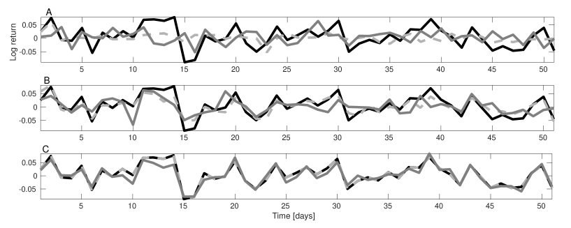
Figure 1: An example reproduction of logarithmic return time-series using the random factor model (dark grey curves) and PCA (dashed light grey curves) compared with the data (solid black curves) using (A) 10 factors, (B) 100 factors, and (C) 500 factors. The data is normalized to have zero average return, as describes in the text.

3.1 Reproduction of time-series

Fig. 1 provides three examples of time-series reproduction using the RFM and PCA. The RFM (grey solid curve in Fig. 1) provides a good reproduction of the single time-series even with a low number of factors. The accuracy of the reproduction improves with the number of factors: the agreement of the RFM and the data is very good with 500 factors.

The number of factors is not limited to the number of time-series in the RFM, since the random factors do not necessarily span the entire space in which time-series may have values. Only in the limit of large number of factors is the entire space covered.

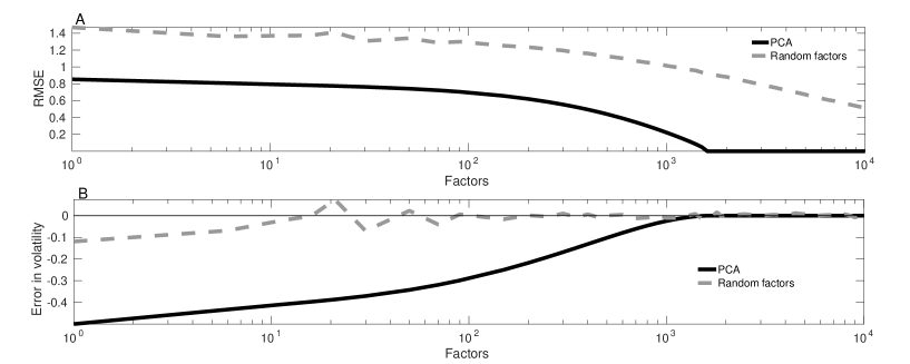
Figure 2: Accuracy of time-series representations. (A) Error in time-series reproduction using the random factor model (dashed gray curve) and PCA (black solid curve) measured by RMSE. Curves are shown as functions of the number of factors. (B) Error in reproduction of time-series volatility using the random factor model (dashed gray curve) and PCA (black solid curve) as a function of the number of factors. Errors are relative to the volatility of the time-series due to normalization.

Both PCA and the RFM provide good reproductions of the data (Fig. 1), however, there are deviations from the data in each reproduction. In the root mean square error (RMSE) sense, PCA gives a better reproduction of the time-series than the RFM (Fig. 2A). RMSE in the reproduction of the entire data set is 0.79 in PCA vs 1.37 in the RFM with 10 factors (Fig. 1A).

3.2 Volatility

The RFM reproduces volatility of the time-series almost exactly even with a small number of factors, while in PCA volatility estimates improve pronouncedly with more factors (Fig. 2B). Since volatility of each time-series is normalized to 1 separately, accuracy of volatility reproduction is relative to volatilities of the underlying time-series in Fig. 2B.

In the RFM, error in volatility is about 3.1 percent of volatility with ten factors. In PCA, error is about 41.7 percent of volatility with ten factors. Accuracy increases until 1,000 factors is reached, after which essentially no error is observed in PCA. While the RFM reproduces the overall volatility of the equity time-series faithfully, it does not capture time-dependence of volatility particularly well (data not shown).

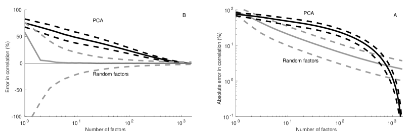
Figure 3: Accuracy of the correlation modeling. (A) Median error (solid gray curves; measured in percentage points) in correlation coefficient estimates in all pairs in the data-set estimated using 1,000 different random factor models, together with the 25th and 75th (dashed gray curves) percentiles of error in correlation estimates. The results are compared with the estimates of correlation based on PCA (solid black curve), together with the 25th and 75th (dashed black curves) percentiles. The results are shown as a function of the number of factors (abscissa). (B) Median absolute error of the random factor model (solid grey curve; measured in percentage points), together with the 25th and 75th percentiles (dashed grey curves); Median error in PCA (solid black curve) and the 25th and 75th percentiles (dashed black curves).

3.3 Correlation coefficient

Fig. 3 shows the accuracy of reproduction of correlation coefficients in all analyzed pairs of stocks. In the RFM, the median error converges rapidly to zero with only a few factors. The 25th and 75th percentiles of error converge toward zero when the number of factors increases. Together these three curves form a funnel (Fig. 3A) that rapidly converges toward zero. This shows that the typical accuracy of the correlation coefficient reproduction improves rapidly with the number of factors. Still, some noise persists even with the “full” set of factors, for $k=d$.

In PCA, median error approaches zero only with around 1,000 factors, which is largely a consequence of PCA significantly underestimating volatilities of time-series. The 25th and 75th percentiles concentrate around the median away from zero in PCA.

Fig. 3B shows results on absolute error in correlation coefficient as a function of the number of factors. In the RFM, correlation estimates converge toward the exact value when the number of factors is increased, however, convergence is less rapid than in analysis shown in Fig. 3A. This is a result of the fact that error can be in either direction in the RFM. Compared with PCA, correlation estimates in the RFM converge significantly more rapidly toward the exact value. Since error is always in the same direction in PCA, there are no differences between absolute error and relative error in PCA-based analyses.

The RFM provides a more accurate description of correlation coefficients than PCA, when the number of factors is less than about 500. Noise inherent in the random factor model has the consequence that the error in correlation estimates does not disappear in the RFM even with the full set of variables even though median estimate rapidly converges toward the observed correlation.

The cross-over to regime where PCA is more accurate occurs around 700–800 factors (Fig. 3). When the number of factors is very high, PCA gives as good as or better correlation coefficients than the median estimate from the RFM. A factor model with this large number of factors is of little use in practical applications.

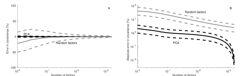
Figure 4: Accuracy of covariance estimation. (A) Median error (solid gray curves; measure in percentage points) in covariance in all pairs in the data-set estimated using 1,000 different random factor models, together with 25th and 75th (dashed gray curves) percentiles of error in covariance estimates. The results are compared with the estimates of covariance based on PCA (solid black curve), together with the 25th and 75th (dashed black curves) percentiles. The results are shown as a function of the number of factors (abscissa). (B) Median absolute error (solid gray curves; measure in percentage points) in covariance in all pairs in the data-set estimated using 1,000 different random factor models, together with the 25th and 75th (dashed gray curves) percentiles of error. The results are compared with the estimates of covariance based on PCA (solid black curve), together with the 25th and 75th (dashed black curves) percentiles.

3.4 Covariance

The median error in covariance estimates converges rapidly toward zero in the RFM. The 25th and 75th percentiles form a funnel that converges toward zero when the number factors increases (Fig. 4A). Despite the fact that PCA is worse than the RFM in reproducing correlation coefficients, PCA gives a better reproduction of the covariance matrix (Fig. 4B).

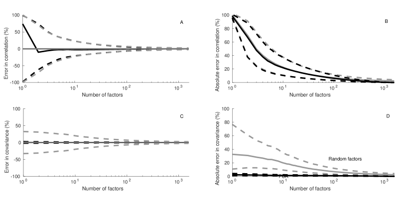
Figure 5: Analysis of the reduced data set in which the influence of the market is removed. (A) Error in correlation coefficient, (B) Absolute error in correlation coefficient estimates, (C) Error in covariance, and (D) Absolute error in covariance estimates in an random factor model (gray curves) and in PCA (black curves). Solid lines are median estimates, dashed lines 25th and 75th percentiles.

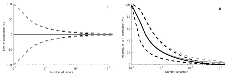
Figure 6: Reproduction of correlation coefficient in randomly-generated data. (A) Error in correlation reproduction of the random data using the random factor model (dashed gray curve) and PCA (black solid curve) . Curves are shown as functions of the number of factors. Differences are in percentage points. (B) Absolute error in correlation reproduction of the random data using the random factor model (dashed gray curve) and PCA (black solid curve) .

3.5 Impact of the market factor

The risk in the equity market is often dominated by a single factor known as the market risk factor (e.g., Sharpe, 1964). To better analyze the other possible risk factors, we subtract the first principal component, corresponding to the market risk factor, from the data and reanalyze the remaining data (the ”reduced data”).

Fig. 5A shows that PCA becomes more accurate in reproducing the correlation coefficients when the impact of the market risk factor is removed from the data. Perhaps more surprisingly, reproduction of data structure becomes equally accurate in the RFM and in PCA with respect to both error measures in the correlation coefficient (Fig. 5A and 5B). This suggests that the RFM and PCA contain equal amounts of information about the correlations.

As a further check, we generated random data by sampling the normal probability distribution $N(0,1)$ repeatedly. Fig. 6 shows that the accuracy of both the RFM and PCA is almost identical in this case. Comparison with Figures 5A and 5B shows that the accuracy of reproduction of the “reduced” Russell correlations does not significantly differ from the accuracy of the random data. This indicates that the fluctuations around the market risk factor are largely a product of independent “noise” contributions.

Removal of the market risk factor from the data also influences the accuracy of covariance reproduction. PCA is again more accurate than the RFM in covariance reproduction (Fig. 5C and 5D). In this case, the median error of covariance matrix reproduction does not deviate from zero in the RFM, and the 25th and 75th percentiles are almost symmetrically around x-axis.

4 Universality

A number of probability distributions have been found useful in the random projection method (e.g., Achlioptas (2003); Kaski (1998)). Matoušek (2008) found that almost any probability distribution with zero mean, unit variance, and subgaussian tail fulfills the requirements of the Johnson-Lindenstrauss theorem. These findings suggest that it may not matter much which probability distribution is used in the random projections. To find out whether this is the case in an RFM, we reanalyze the data using RFMs based on six different probability distributions. We have also discussed some lowest order effects of varying the probability distribution, as well as reasons why deviation from a Gaussian distribution leads only to small corrections, in Remark A.4 after the proof in the Appendix.

4.1 Probability distributions

The six probability distributions that we employ here are two sparse matrix models of Achlioptas (2003), a column-normalized Gaussian model, a row-normalized Gaussian model, the baseline Gaussian model (defined in Sec. 2.4) and a uniform model. In each case, the probability distribution is symmetric with respect to the origin and such that the expectation is zero. Each probability distribution also has a subgaussian tail. These RFMs differ from the baseline Gaussian RFM only by the construction of the random projection matrix $B$, and by the normalization.

4.1.1 Coin-flipping distributions

The simplest specification for random projection is the ”random coin-flipping” algorithm of Achlioptas (2003). It is defined by choosing each element $B_{pq}$ of matrix $B$ independently according to rule: set $B_{pq}=+1$ with probability 0.5 and set $B_{pq}=-1$ with probability 0.5.

The second random projection that Achlioptas (2003) proposes is based on a more sparse projection matrix defined by: set $B_{pq}=+1$ with probability 1/6, set $B_{pq}=0$ with probability 2/3 and set $B_{pq}=-1$ with probability 1/6. Again each element is chosen independently of the other elements. Based on these random projections, we can define two RFMs.

4.1.2 Gaussian and uniform distributions

In addition to the baseline Gaussian RFM, we analyze two different RFMs based on the normal distribution. In the first RFM, matrix $B$ is based on the spherical uniform distribution. The elements of matrix $B$ are defined by

$$B_{ml}=z_{ml}/Z,$$ (16)

where $z_{ml}\sim N(0,1)$ are indendent and $Z=\sqrt{\sum\nolimits_{p}|z_{pl}|^{2}}$. In this RFM, columns of matrix $B$ are normalized in such a way that their length is exactly one.

Due to normalization of the columns of matrix $B$, diagonal elements of matrix $B^{T}B\in{\mathbb{R}}^{d\times d}$ behave as in an orthogonal matrix. Then $(B^{T}B)_{mm}=1$ for all $m=1,2,\ldots,k$. Non-diagonal elements of $B^{T}B$ have zero expectation and variance proportional to $1/d$ (Kaski, 1998). Hence, non-diagonal elements of $B^{T}B$ are approximately distributed according to zero-mean normal distribution at a relatively low dimension. Therefore $B^{T}B=1+\epsilon$, where $\epsilon\in{\mathbb{R}}^{d\times d}$ has non-zero elements only on off-diagonal, $\mathbbm{E}[\epsilon]=0$ and $|\mathbbm{E}[\epsilon]|<2/d$. Matrix $B$ is then almost orthonormal.

The second RFM based on the Gaussian probability distribution is a variation on the theme: Instead of column-normalization in the first model, rows of projection matrix $B$ are normalized to unit length. This is the only difference between the two RFMs, but it is sufficient to require a different normalization constant.

The sixth considered RFM is defined by projection matrix B, which is based on the continuous uniform probability distribution. Each element in the projection matrix $B$ is chosen independently from the uniform distribution on interval $[-1,1]$, that is, $B_{mn}\sim U(-1,1)$ for each $m,n$.

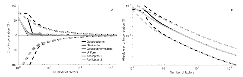
Figure 7: Comparison of six different projection matrix specifications. Solid lines are median estimates, dashed lines the 25th and 75th percentiles. (A) Error in correlation coefficient estimates as functions of the number of factors in six models. Error is computed from the entire set of correlation pairs in 1,591 time-series. (B) Absolute error in correlation coefficient estimates in the six models as functions of the number of factors.

4.2 Universality of distributions

Fig. 7 shows that all six RFMs produce almost equally accurate results. To reduce noise, Fig. 7 shows results averaged over 50 sample runs. When the number of factors exceeds 10, all RFMs produce almost identical median accuracy. The only deviation is the column-normalized Gaussian model, which deviates from the other RFMs when the number of factors is less than 5. All the other RFMs produce identical results also in this regime. The accuracy of the 25th and 75th percentiles mainly depends on the number of factors, not much on the way factors are generated.

The results suggest that the details of how the projection matrix is specified are not that important. Almost any sufficiently regular construction of the random projection matrix (when properly normalized) produces a factor model, which preserves the approximate correlation structure. The main requirement here seems to be that matrix elements are chosen randomly and independently of other matrix elements. This supports the view that the RFM represents quite well how the bulk of factor models would describe the analyzed task.

5 Discussion

5.1 Randomness of factors

We set out to analyze the impact of random selection of factors on a linear factor model. We were interested in whether and how randomness in the choice of factors impacts the reproduction of long equity time-series and, in particular, whether their interdependence is preserved. We found that accuracy of a typical random factor model is respectable, especially the correlation matrix is well-preserved in the reproduction of time-series (Section 4). We also derived novel theoretical results on the accuracy of a random factor model (Appendix A).

It may seem unlikely that a factor model with randomly-chosen factors could be used for any kind of factor modeling. One of the reasons for the ability of an RFM to capture the details of an equity time-series resides in the fact that random factors are, as a consequence of independence of elements, almost orthogonal to each other. Furthermore, the number of almost orthogonal vectors is higher in a higher-dimensional space, which reduces the impact of the ”curse of dimensionality” (Bellman, 1957; Indyk and Motwani, 1998) and thereby makes data represention more feasible. A suitably high number of random factors will then span a subspace sufficient to capture the return time-series at the desired accuracy.

On the other hand, the number of factors is not bounded in a random factor model. Only in the limit of infinite number of factors, an RFM is ensured to reproduce the original time-series perfectly. This can be viewed as a disadvantage of using an RFM.

5.2 Universality

In a classical factor model, only a few factors are statistically significant. Then, explanatory power of each factor should be large. In a statistical factor model, a larger number of factors is often used, which also has the consequence that a larger ambiguity in the choice of factors is encountered (Ledoit and Wolf, 2004). Several different sets of factors may provide almost equally good fit to the data. In an RFM, each factor has only a small explanatory power, which suggests that a large number of factor sets provide essentially equally good descriptions of the data and its structure. This was observed in our computational experiments.

The number of random factors seems to be more important than fine-tuning of random factor time-series. The way an RFM is constructed is not important as long as elements of projection $B$ are independently drawn from a suitably regular probability distribution with zero expectation and subgaussian tails. Regardless of the probability distribution used, we obtained almost identically accurate results. These findings suggest that a kind of universality of RFMs is present, at least with respect to correlation coefficients. The results are largely dominated by a set of typical RFMs that have a rather similar accuracy of data reproduction. We have called this set of factor models the bulk.

The analysis of the proof of Theorem A.1 (see Remark A.4) supports the view that universality is present with respect to probability distributions. The assumption that probability distribution is Gaussian is not necessarily required in the theorem. It suffices to assume independence of the random matrix elements, and it is likely that this requirement can be relaxed further.

5.3 Accuracy, revisited

In our analyses, we employed PCA as a yardstick against which we compared the RFM. The RFM described correlation structures and volatility well, but individual data points of time-series were reproduced less accurately. PCA reproduced individual data points of time-series more accurately, but reproduction of cross-correlations of the time-series was not that good mainly due to underestimated volatility. In other words, the RFM preserved the structure of the data but not necessarily the details of single time-series, while PCA representation preserved the details but not necessarily the correlation structure.

It is worth pointing out that PCA is fitted to preserve co-variance of time-series, not correlations. An RFM is fitted in no way to the data, so the preservation of correlations is quite unexpected.

The previous literature has compared the performance of the random projection method with PCA, and found results similar to ours. Bingham and Mannila (2001) found that random projection method performed significantly better than PCA in the compression of image data and in text clustering. Goal et al. (2005) found that random projection compares favorably with PCA, although PCA is more accurate with small number of dimensions. Tang et al. (2005) found that in text clustering a PCA-based method provides better accuracy with small number of dimensions, while with high number of dimensions the random projection method dominated. Deegalla and Bostrom (2006) found that in five image data sets and five micro array data sets, PCA dominated with a small number of dimensions but its performance deteriorated when the dimensions of the data increased (cross-over occurs at 15–150 dimensions depending on the data set), while random projection dominates at high number of dimensions. Our findings are consistent with the results of these previous studies.

The realm of RFMs is the domain of huge data sets consisting of large number of long time-series. An RFM answers the question: how many factors will a generic linear factor model require to describe the data at a specific accuracy.

Appendix A Accuracy of random factor approach

We prove here the following result about the mean and variance of the projection operators involved in the random factor models.

Theorem A.1

Suppose $k\geq 1$, $d\geq 2$ and that the matrix elements of the random matrix $B\in{\mathbb{R}}^{k\times d}$ are i.i.d. and $N(0,1)$-distributed. For some given $a>0$ define a new random matrix $P\in{\mathbb{R}}^{d\times d}$ by $P:=aB^{T}B$.

Then for every non-random vectors $u,v\in{\mathbb{R}}^{d}$ all of the following results hold:

1. $\mathbbm{E}\!\left[(Pu)_{m}\right]=aku_{m}$ for all $m$, and $\mathbbm{E}[\mu_{Pu}]=ak\mu_{u}$.

2. $\operatorname*{Var}((Pu)_{m})=a^{2}k\left(u_{m}^{2}+|u|^{2}\right)$ for all $m$.

3. $\mathbbm{E}\!\left[C_{Pu,Pv}\right]=a^{2}k(d+k)C_{u,v}+a^{2}kd\mu_{u}\mu_{v}$.

4. If $\mu_{u}=\mu_{v}=0$ and $d\geq 4$, then $\operatorname*{Var}\!\left(C_{Pu,Pv}\right)\leq a^{4}8k(k+d)^{2}\sigma_{u}^{2}\sigma_{v}^{2}$.

The main application of the theorem is the following consequence of the above result:

Corollary A.2

Suppose $k\geq 1$, $d\geq 4$ and that the matrix elements of the random matrix $B\in{\mathbb{R}}^{k\times d}$ are i.i.d. and $N(0,1)$-distributed. Set $a=[k(k+d)]^{-1/2}$ and define $P=aB^{T}B$.

Then for every $b>0$ and non-random vectors $u,v\in{\mathbb{R}}^{d}$, with $\mu_{u}=\mu_{v}=0$, all of the following results hold:

1. $\mathbbm{E}\!\left[(Pu)_{m}\right]=\left[k/(k+d)\right]^{1/2}u_{m}$ for all $m$ and $\mathbbm{E}[\mu_{Pu}]=0$.

2. $\operatorname*{Var}((Pu)_{m})=\left(u_{m}^{2}+(d-1)\sigma_{u}^{2}\right)/(d+k)$ for all $m$.

3. $\mathbbm{E}\!\left[C_{Pu,Pv}\right]=C_{u,v}$.

4. $\mathbbm{P}\!\left[|C_{Pu,Pv}-C_{u,v}|\geq b\right]\leq\frac{8}{kb^{2}}\sigma_{u}^{2}\sigma_{v}^{2}$.

Proof of the Corollary:  With the added assumptions $\mu_{u}=\mu_{v}=0$, the definition of the sample variance yields the identities $|u|^{2}=(d-1)\sigma_{u}^{2}$ and $|v|^{2}=(d-1)\sigma_{v}^{2}$. Thus items 1, 2 and 3 are immediate corollaries using $a^{2}=1/(k(d+k))$. On the other hand, if we denote the standard deviation of $C_{Pu,Pv}$ by $S$, then by Chebyshev’s inequality we have $\mathbbm{P}\!\left[|C_{Pu,Pv}-C_{u,v}|\geq cS\right]\leq c^{-2}$ for any $c>0$. Applying this with $c:=b/S$ thus implies $\mathbbm{P}\!\left[|C_{Pu,Pv}-C_{u,v}|\geq b\right]\leq S^{2}b^{-2}$. Hence, item 4 of the Theorem implies the bound in the last item of the Corollary.

Proof of the Theorem:  Assume $k,d,B,a,P,u,v$ be given as in the theorem, and define $Z:=Pu$, $Z^{\prime}:=Pv$ and $C:=C_{Pu,Pv}$. $Z_{m}$, $Z^{\prime}_{m}$, $m=1,2,\ldots,d$, and $C$ are then all real-valued random variables.

The following results could also be proven by straightforward but rather lengthy direct estimates relying on Wick’s product rule, i.e., Isserlis’ theorem, valid for the present Gaussian random variables $B_{jm}$. A better control of the associated combinatorics is obtained by using Wick polynomial expansions instead. For the present case of Gaussian random variables Wick polynomials reduce to Hermite polynomials; Appendix A of (Lukkarinen and Marcozzi, 2016) provides a quick summary of the definition and main properties of general Wick polynomials, and we refer to Janson (1997); Peccati and Taqqu (2011); Lukkarinen et al. (2016) for more detailed expositions.

We rely on the following Wick polynomial expansion of arbitrary centered expectations of monomials of random variables: for any product of random variables $x_{1},x_{2},\ldots,x_{n}$, with the corresponding index set $I=\{1,2,\ldots,n\}$, one has

$$\prod_{i=1}^{n}x_{i}-\mathbbm{E}\biggl{[}\prod_{i=1}^{n}x_{i}\biggr{]}=\sum_{\emptyset\neq E\subset I}\mathbbm{E}\biggl{[}\prod_{i\in I\setminus E}x_{i}\biggr{]}\mathop{:}\nolimits\!\prod_{i\in E}x_{i}\!\mathop{:}\nolimits\,.$$ (17)

For any $m=1,2,\ldots,d$, the definitions yield

$$Z_{m}=(Pu)_{m}=a\sum_{n=1}^{d}\sum_{j=1}^{k}B_{jm}B_{jn}u_{n}\,.$$ (18)

Since $B_{jm}$ are i.i.d. centered, normalized Gaussian, this implies

$$\mathbbm{E}[Z_{m}]=a\sum_{n=1}^{d}\sum_{j=1}^{k}{\mathbbm{1}}_{\{n=m\}}u_{n}=aku_{m}\,,$$ (19)

where ${\mathbbm{1}}_{\{n=m\}}$ stands for an indicator function having value $1$, when $n=m$, and $0$ otherwise. Thus $\mathbbm{E}[\mu_{Pu}]=\frac{1}{d}\sum_{n=1}^{d}\mathbbm{E}[Z_{m}]=ak\mu_{u}$ As $\mathbbm{E}[B_{jm}]=0$, centering the variable $Z_{m}$ yields the following simple Wick polynomial expansion:

$$Z_{m}-\mathbbm{E}[Z_{m}]=a\sum_{n=1}^{d}u_{n}\sum_{j=1}^{k}\mathop{:}\nolimits\!B_{jm}B_{jn}\!\mathop{:}\nolimits\,.$$ (20)

The usefulness of Wick polynomials lies in the property that their products satisfy the same moments-to-cumulants expansion as simple products, with the additional rule that any partition with a cluster of indices inside one of the Wick polynomials will be missing from the expansion. For instance, for any random variables $x_{1},x_{2},x_{3},x_{4}$—which need not be independent nor Gaussian—one has

$$\mathbbm{E}[\mathop{:}\nolimits\!x_{1}x_{2}\!\mathop{:}\nolimits\mathop{:}\nolimits\!x_{3}x_{4}\!\mathop{:}\nolimits]=\kappa[x_{1},x_{2},x_{3},x_{4}]+\kappa[x_{1},x_{3}]\kappa[x_{2},x_{4}]+\kappa[x_{1},x_{4}]\kappa[x_{2},x_{3}]\,,$$ (21)

where $\kappa$ denotes a cumulant. Here, for instance, $\kappa[x_{1},x_{3}]=\operatorname*{Cov}(x_{1},x_{3})$. Applying this to the $B$-variables yields

$$\mathbbm{E}[\mathop{:}\nolimits\!B_{jm}B_{jn}\!\mathop{:}\nolimits\mathop{:}\nolimits\!B_{j^{\prime}m^{\prime}}B_{j^{\prime}n^{\prime}}\!\mathop{:}\nolimits]={\mathbbm{1}}_{\{j^{\prime}=j,m^{\prime}=m\}}{\mathbbm{1}}_{\{j^{\prime}=j,n^{\prime}=n\}}+{\mathbbm{1}}_{\{j^{\prime}=j,n^{\prime}=m\}}{\mathbbm{1}}_{\{j^{\prime}=j,n=m^{\prime}\}}\,,$$ (22)

since for Gaussian random variables the fourth cumulant is equal to zero. Therefore, by (20) and (22), we have

$$\operatorname*{Cov}(Z_{m},Z^{\prime}_{m^{\prime}})=\mathbbm{E}[(Z_{m}-\mathbbm{E}[Z_{m}])(Z^{\prime}_{m^{\prime}}-\mathbbm{E}[Z^{\prime}_{m^{\prime}}])]$$

$$\quad=a^{2}\sum_{n^{\prime},n=1}^{d}u_{n}v_{n^{\prime}}\sum_{j^{\prime},j=1}^{k}\mathbbm{E}[\mathop{:}\nolimits\!B_{jm}B_{jn}\!\mathop{:}\nolimits\mathop{:}\nolimits\!B_{j^{\prime}m^{\prime}}B_{j^{\prime}n^{\prime}}\!\mathop{:}\nolimits]$$

$$\quad=a^{2}\left(k{\mathbbm{1}}_{\{m^{\prime}=m\}}\sum_{n=1}^{d}u_{n}v_{n}+ku_{m^{\prime}}v_{m}\right)=a^{2}k\left({\mathbbm{1}}_{\{m^{\prime}=m\}}u\cdot v+u_{m^{\prime}}v_{m}\right)\,,$$ (23)

and thus, in particular,

$$\operatorname*{Var}(Z_{m})=\mathbbm{E}[(Z_{m}-\mathbbm{E}[Z_{m}])^{2}]=a^{2}k\left(|u|^{2}+u_{m}^{2}\right)\,.$$ (24)

Therefore, we have now proven the first two items of the Theorem.

The combinatorics gets progressively heavier in the remaining two items. Let us begin with the scalar product

$$Pu\cdot Pv=Z\cdot Z^{\prime}=\sum_{m=1}^{d}Z_{m}Z^{\prime}_{m}=\sum_{m=1}^{d}z_{m}z^{\prime}_{m}+ak\sum_{m=1}^{d}(u_{m}z^{\prime}_{m}+v_{m}z_{m})+a^{2}k^{2}\sum_{m=1}^{d}u_{m}v_{m}\,,$$ (25)

where $z_{m}=Z_{m}-\mathbbm{E}[Z_{m}]=Z_{m}-aku_{m}$, $z^{\prime}_{m}=Z^{\prime}_{m}-\mathbbm{E}[Z^{\prime}_{m}]=Z^{\prime}_{m}-akv_{m}$ denote the centered variables. Taking an expectation and using (A) for $m^{\prime}=m$ thus yields

$$\mathbbm{E}[Pu\cdot Pv]=\sum_{m=1}^{d}a^{2}k\left(u\cdot v+u_{m}v_{m}\right)+a^{2}k^{2}u\cdot v=a^{2}k(d+1+k)u\cdot v\,.$$ (26)

The definition of $C$ reads explicitly

$$C=C_{Pu,Pv}=\frac{1}{d-1}\sum_{m=1}^{d}(Pu)_{m}(Pv)_{m}-\frac{d}{d-1}\mu_{Pu}\mu_{Pv}=\frac{1}{d-1}Z\cdot Z^{\prime}-\frac{d}{d-1}\mu_{Z}\mu_{Z^{\prime}}\,.$$ (27)

To compute its expectation, we still need to evaluate

$$\mathbbm{E}[\mu_{Z}\mu_{Z^{\prime}}]=\operatorname*{Cov}[\mu_{Z},\mu_{Z^{\prime}}]+\mathbbm{E}[\mu_{Z}]\mathbbm{E}[\mu_{Z^{\prime}}]=\frac{1}{d^{2}}\sum_{m^{\prime},m=1}^{d}\operatorname*{Cov}[Z_{m},Z^{\prime}_{m^{\prime}}]+a^{2}k^{2}\mu_{u}\mu_{v}$$

$$\quad=\frac{a^{2}k}{d^{2}}\sum_{m^{\prime},m=1}^{d}\left({\mathbbm{1}}_{\{m^{\prime}=m\}}u\cdot v+u_{m^{\prime}}v_{m}\right)+a^{2}k^{2}\mu_{u}\mu_{v}=\frac{a^{2}k}{d}u\cdot v+a^{2}k(k+1)\mu_{u}\mu_{v}\,.$$ (28)

Therefore,

$$\mathbbm{E}[C]=\frac{a^{2}k}{d-1}(d+k)u\cdot v-\frac{d}{d-1}a^{2}k(k+1)\mu_{u}\mu_{v}=a^{2}k(d+k)C_{u,v}+a^{2}kd\mu_{u}\mu_{v}\,,$$ (29)

where in the last step we have used the identity $u\cdot v=(d-1)C_{u,v}+d\mu_{u}\mu_{v}$.

For the final result, let us assume in addition that $\mu_{u}=\mu_{v}=0$. To avoid iterated Wick polynomials, let us begin with $C=\frac{1}{d-1}Z\cdot Z^{\prime}-\frac{d}{d-1}\mu_{Z}\mu_{Z^{\prime}}$ and express the two terms separately in Wick form. Namely, now

$$\mu_{Z}\mu_{Z^{\prime}}=\frac{a^{2}}{d^{2}}\sum_{n^{\prime},n=1}^{d}v_{n^{\prime}}u_{n}\sum_{m^{\prime},m=1}^{d}\sum_{j^{\prime},j=1}^{k}B_{jm}B_{jn}B_{j^{\prime}m^{\prime}}B_{j^{\prime}n^{\prime}}\,,$$ (30)

where the product of four $B$-factors can be expanded using Wick polynomial expansion (17). Since only expectations of products of even number of $B$:s can be non-zero, we obtain

$$B_{jm}B_{jn}B_{j^{\prime}m^{\prime}}B_{j^{\prime}n^{\prime}}-\mathbbm{E}[B_{jm}B_{jn}B_{j^{\prime}m^{\prime}}B_{j^{\prime}n^{\prime}}]$$

$$\quad=\mathop{:}\nolimits\!B_{jm}B_{jn}B_{j^{\prime}m^{\prime}}B_{j^{\prime}n^{\prime}}\!\mathop{:}\nolimits+\mathbbm{E}[B_{jm}B_{jn}]\mathop{:}\nolimits\!B_{j^{\prime}m^{\prime}}B_{j^{\prime}n^{\prime}}\!\mathop{:}\nolimits+\mathbbm{E}[B_{jm}B_{j^{\prime}m^{\prime}}]\mathop{:}\nolimits\!B_{jn}B_{j^{\prime}n^{\prime}}\!\mathop{:}\nolimits$$

$$\qquad+\mathbbm{E}[B_{jm}B_{j^{\prime}n^{\prime}}]\mathop{:}\nolimits\!B_{jn}B_{j^{\prime}m^{\prime}}\!\mathop{:}\nolimits+\mathbbm{E}[B_{jn}B_{j^{\prime}m^{\prime}}]\mathop{:}\nolimits\!B_{jm}B_{j^{\prime}n^{\prime}}\!\mathop{:}\nolimits$$

$$\qquad+\mathbbm{E}[B_{jn}B_{j^{\prime}n^{\prime}}]\mathop{:}\nolimits\!B_{jm}B_{j^{\prime}m^{\prime}}\!\mathop{:}\nolimits+\mathbbm{E}[B_{j^{\prime}m^{\prime}}B_{j^{\prime}n^{\prime}}]\mathop{:}\nolimits\!B_{jm}B_{jn}\!\mathop{:}\nolimits$$

$$\quad=\mathop{:}\nolimits\!B_{jm}B_{jn}B_{j^{\prime}m^{\prime}}B_{j^{\prime}n^{\prime}}\!\mathop{:}\nolimits+{\mathbbm{1}}_{\{m=n\}}\mathop{:}\nolimits\!B_{j^{\prime}m^{\prime}}B_{j^{\prime}n^{\prime}}\!\mathop{:}\nolimits+{\mathbbm{1}}_{\{m^{\prime}=n^{\prime}\}}\mathop{:}\nolimits\!B_{jm}B_{jn}\!\mathop{:}\nolimits$$

$$\qquad+{\mathbbm{1}}_{\{j^{\prime}=j\}}\bigl{[}{\mathbbm{1}}_{\{m=m^{\prime}\}}\mathop{:}\nolimits\!B_{jn}B_{jn^{\prime}}\!\mathop{:}\nolimits+{\mathbbm{1}}_{\{m=n^{\prime}\}}\mathop{:}\nolimits\!B_{jn}B_{jm^{\prime}}\!\mathop{:}\nolimits+{\mathbbm{1}}_{\{m^{\prime}=n\}}\mathop{:}\nolimits\!B_{jm}B_{jn^{\prime}}\!\mathop{:}\nolimits+{\mathbbm{1}}_{\{n=n^{\prime}\}}\mathop{:}\nolimits\!B_{jm}B_{jm^{\prime}}\!\mathop{:}\nolimits\bigr{]}$$ (31)

Therefore,

$$\mu_{Z}\mu_{Z^{\prime}}-\mathbbm{E}[\mu_{Z}\mu_{Z^{\prime}}]=\frac{a^{2}}{d^{2}}\sum_{n^{\prime},n=1}^{d}v_{n^{\prime}}u_{n}\sum_{m^{\prime},m=1}^{d}\sum_{j^{\prime},j=1}^{k}\mathop{:}\nolimits\!B_{jm}B_{jn}B_{j^{\prime}m^{\prime}}B_{j^{\prime}n^{\prime}}\!\mathop{:}\nolimits$$

$$\qquad+\frac{a^{2}}{d}\sum_{n^{\prime},n=1}^{d}v_{n^{\prime}}u_{n}\sum_{j=1}^{k}\mathop{:}\nolimits\!B_{jn}B_{jn^{\prime}}\!\mathop{:}\nolimits+\frac{a^{2}}{d}\frac{d-1}{d}C_{u,v}\sum_{m^{\prime},m=1}^{d}\sum_{j=1}^{k}\mathop{:}\nolimits\!B_{jm}B_{jm^{\prime}}\!\mathop{:}\nolimits\,,$$ (32)

where we have applied the assumptions $\mu_{u}=0=\mu_{v}$.

Similarly, since

$$\frac{1}{d-1}Z\cdot Z^{\prime}=\frac{a^{2}}{d-1}\sum_{n^{\prime},n=1}^{d}v_{n^{\prime}}u_{n}\sum_{m=1}^{d}\sum_{j^{\prime},j=1}^{k}B_{jm}B_{jn}B_{j^{\prime}m}B_{j^{\prime}n^{\prime}}\,,$$ (33)

and by (A)

$$B_{jm}B_{jn}B_{j^{\prime}m}B_{j^{\prime}n^{\prime}}-\mathbbm{E}[B_{jm}B_{jn}B_{j^{\prime}m}B_{j^{\prime}n^{\prime}}]$$

$$\quad=\mathop{:}\nolimits\!B_{jm}B_{jn}B_{j^{\prime}m}B_{j^{\prime}n^{\prime}}\!\mathop{:}\nolimits+{\mathbbm{1}}_{\{m=n\}}\mathop{:}\nolimits\!B_{j^{\prime}m}B_{j^{\prime}n^{\prime}}\!\mathop{:}\nolimits+{\mathbbm{1}}_{\{m=n^{\prime}\}}\mathop{:}\nolimits\!B_{jm}B_{jn}\!\mathop{:}\nolimits$$

$$\qquad+{\mathbbm{1}}_{\{j^{\prime}=j\}}\bigl{[}\mathop{:}\nolimits\!B_{jn}B_{jn^{\prime}}\!\mathop{:}\nolimits+{\mathbbm{1}}_{\{m=n^{\prime}\}}\mathop{:}\nolimits\!B_{jn}B_{jm}\!\mathop{:}\nolimits+{\mathbbm{1}}_{\{m=n\}}\mathop{:}\nolimits\!B_{jm}B_{jn^{\prime}}\!\mathop{:}\nolimits+{\mathbbm{1}}_{\{n=n^{\prime}\}}\mathop{:}\nolimits\!B_{jm}B_{jm}\!\mathop{:}\nolimits\bigr{]}\,,$$ (34)

we obtain a Wick polynomial expansion

$$\frac{1}{d-1}Z\cdot Z^{\prime}-\mathbbm{E}\left[\frac{1}{d-1}Z\cdot Z^{\prime}\right]=\frac{a^{2}}{d-1}\sum_{n^{\prime},n=1}^{d}v_{n^{\prime}}u_{n}\sum_{m=1}^{d}\sum_{j^{\prime},j=1}^{k}\mathop{:}\nolimits\!B_{jm}B_{jn}B_{j^{\prime}m}B_{j^{\prime}n^{\prime}}\!\mathop{:}\nolimits$$

$$\qquad+\frac{a^{2}}{d-1}(2k+d+2)\sum_{n^{\prime},n=1}^{d}v_{n^{\prime}}u_{n}\sum_{j=1}^{k}\mathop{:}\nolimits\!B_{jn}B_{jn^{\prime}}\!\mathop{:}\nolimits+a^{2}C_{u,v}\sum_{m=1}^{d}\sum_{j=1}^{k}\mathop{:}\nolimits\!B_{jm}B_{jm}\!\mathop{:}\nolimits\,.$$ (35)

Combining the above results together finally yields a Wick polynomial expansion for the centered $C$,

$$C-\mathbbm{E}[C]=\frac{a^{2}}{d-1}\sum_{n^{\prime},n=1}^{d}v_{n^{\prime}}u_{n}\sum_{m=1}^{d}\sum_{j^{\prime},j=1}^{k}\mathop{:}\nolimits\!B_{jm}B_{jn}B_{j^{\prime}m}B_{j^{\prime}n^{\prime}}\!\mathop{:}\nolimits$$

$$\qquad-\frac{a^{2}}{d(d-1)}\sum_{n^{\prime},n=1}^{d}v_{n^{\prime}}u_{n}\sum_{m^{\prime},m=1}^{d}\sum_{j^{\prime},j=1}^{k}\mathop{:}\nolimits\!B_{jm}B_{jn}B_{j^{\prime}m^{\prime}}B_{j^{\prime}n^{\prime}}\!\mathop{:}\nolimits$$

$$\qquad+\frac{a^{2}}{d-1}(2k+d+1)\sum_{n^{\prime},n=1}^{d}v_{n^{\prime}}u_{n}\sum_{j=1}^{k}\mathop{:}\nolimits\!B_{jn}B_{jn^{\prime}}\!\mathop{:}\nolimits$$

$$\qquad+a^{2}C_{u,v}\sum_{m=1}^{d}\sum_{j=1}^{k}\mathop{:}\nolimits\!B_{jm}B_{jm}\!\mathop{:}\nolimits-\frac{a^{2}}{d}C_{u,v}\sum_{m^{\prime},m=1}^{d}\sum_{j=1}^{k}\mathop{:}\nolimits\!B_{jm}B_{jm^{\prime}}\!\mathop{:}\nolimits\,.$$ (36)

We use this formula to compute $\operatorname*{Var}(C)=\mathbbm{E}[(C-\mathbbm{E}[C])^{2}]$. In the expanded formula terms containing a product of different degree Wick polynomials yield zero since whatever three pairings is used for the six $B$-factors, one of these pairings connects two elements inside the degree four Wick polynomial. Hence, for instance, $\mathbbm{E}[\mathop{:}\nolimits\!B_{j_{1}m_{1}}B_{j_{1}n_{1}}B_{j^{\prime}_{1}m^{\prime}_{1}}B_{j^{\prime}_{1}n^{\prime}_{1}}\!\mathop{:}\nolimits\mathop{:}\nolimits\!B_{j_{2}m_{2}}B_{j_{2}m^{\prime}_{2}}\!\mathop{:}\nolimits]=0$.

The products of second order terms turn out to yield the dominant contribution. After first taking out a factor $a^{4}d^{-2}(d-1)^{-2}$, it reads explicitly

$$\mathbbm{E}\biggl{[}\biggl{(}d(2k+d+1)\sum_{n^{\prime},n=1}^{d}v_{n^{\prime}}u_{n}\sum_{j=1}^{k}\mathop{:}\nolimits\!B_{jn}B_{jn^{\prime}}\!\mathop{:}\nolimits+du\cdot v\sum_{m=1}^{d}\sum_{j=1}^{k}\mathop{:}\nolimits\!B_{jm}B_{jm}\!\mathop{:}\nolimits-u\cdot v\sum_{m^{\prime},m=1}^{d}\sum_{j=1}^{k}\mathop{:}\nolimits\!B_{jm}B_{jm^{\prime}}\!\mathop{:}\nolimits\biggr{)}^{2}\biggr{]}$$

$$\quad=d^{2}(2k+d+1)^{2}\sum_{n^{\prime}_{1},n_{1},n^{\prime}_{2},n_{2}=1}^{d}v_{n^{\prime}_{1}}u_{n_{1}}v_{n^{\prime}_{2}}u_{n_{2}}\sum_{j_{1},j_{2}=1}^{k}\mathbbm{E}[\mathop{:}\nolimits\!B_{j_{1}n_{1}}B_{j_{1}n^{\prime}_{1}}\!\mathop{:}\nolimits\mathop{:}\nolimits\!B_{j_{2}n_{2}}B_{j_{2}n^{\prime}_{2}}\!\mathop{:}\nolimits]$$

$$\qquad+d^{2}(u\cdot v)^{2}\sum_{m_{1},m_{2}=1}^{d}\sum_{j_{1},j_{2}=1}^{k}\mathbbm{E}[\mathop{:}\nolimits\!B_{j_{1}m_{1}}B_{j_{1}m_{1}}\!\mathop{:}\nolimits\mathop{:}\nolimits\!B_{j_{2}m_{2}}B_{j_{2}m_{2}}\!\mathop{:}\nolimits]$$

$$\qquad+(u\cdot v)^{2}\sum_{m^{\prime}_{1},m_{1},m^{\prime}_{2},m_{2}=1}^{d}\sum_{j_{1},j_{2}=1}^{k}\mathbbm{E}[\mathop{:}\nolimits\!B_{j_{1}m_{1}}B_{j_{1}m^{\prime}_{1}}\!\mathop{:}\nolimits\mathop{:}\nolimits\!B_{j_{2}m_{2}}B_{j_{2}m^{\prime}_{2}}\!\mathop{:}\nolimits]$$

$$\qquad+2d^{2}(2k+d+1)u\cdot v\sum_{n^{\prime},n=1}^{d}v_{n^{\prime}}u_{n}\sum_{j,j_{2}=1}^{k}\sum_{m_{2}=1}^{d}\mathbbm{E}[\mathop{:}\nolimits\!B_{jn}B_{jn^{\prime}}\!\mathop{:}\nolimits\mathop{:}\nolimits\!B_{j_{2}m_{2}}B_{j_{2}m_{2}}\!\mathop{:}\nolimits]$$

$$\qquad-2d(2k+d+1)u\cdot v\sum_{n^{\prime},n=1}^{d}v_{n^{\prime}}u_{n}\sum_{j,j_{2}=1}^{k}\sum_{m_{2}.m^{\prime}_{2}=1}^{d}\mathbbm{E}[\mathop{:}\nolimits\!B_{jn}B_{jn^{\prime}}\!\mathop{:}\nolimits\mathop{:}\nolimits\!B_{j_{2}m_{2}}B_{j_{2}m^{\prime}_{2}}\!\mathop{:}\nolimits]$$

$$\qquad-2d(u\cdot v)^{2}\sum_{j,j_{2}=1}^{k}\sum_{m,m_{2}.m^{\prime}_{2}=1}^{d}\mathbbm{E}[\mathop{:}\nolimits\!B_{jm}B_{jm}\!\mathop{:}\nolimits\mathop{:}\nolimits\!B_{j_{2}m_{2}}B_{j_{2}m^{\prime}_{2}}\!\mathop{:}\nolimits],$$ (37)

which simplifies to

$$d^{2}(2k+d+1)^{2}k(|u|^{2}|v|^{2}+(u\cdot v)^{2})+2d^{2}(u\cdot v)^{2}dk+2(u\cdot v)^{2}kd^{2}$$

$$\qquad+4d^{2}k(2k+d+1)(u\cdot v)^{2}-0-4d^{2}k(u\cdot v)^{2}$$

$$\quad=d^{2}(2k+d+1)^{2}k|u|^{2}|v|^{2}+[d^{2}(2k+d+1)^{2}k+2d^{3}k+2d^{2}k+4d^{2}k(2k+d)](u\cdot v)^{2}\,.$$ (38)

In the remaining products, the allowed pairings are in one-to-one correspondence to permutations where each factor in the left product is paired with the factor in its “permuted” position in the right product. Thus for order four terms we obtain a sum over $4!=24$ terms, namely,

$$\mathbbm{E}[\mathop{:}\nolimits\!B_{j_{1}m_{1}}B_{j_{1}n_{1}}B_{j^{\prime}_{1}m^{\prime}_{1}}B_{j^{\prime}_{1}n^{\prime}_{1}}\!\mathop{:}\nolimits\mathop{:}\nolimits\!B_{j_{2}m_{2}}B_{j_{2}n_{2}}B_{j^{\prime}_{2}m^{\prime}_{2}}B_{j^{\prime}_{2}n^{\prime}_{2}}\!\mathop{:}\nolimits]$$

$$\quad={\mathbbm{1}}_{\{j_{1}=j_{2},j^{\prime}_{1}=j^{\prime}_{2}\}}\bigl{[}{\mathbbm{1}}_{\{m_{1}=m_{2},n_{1}=n_{2}\}}+{\mathbbm{1}}_{\{m_{1}=n_{2},n_{1}=m_{2}\}}\bigr{]}\times\bigl{[}{\mathbbm{1}}_{\{m^{\prime}_{1}=m^{\prime}_{2},n^{\prime}_{1}=n^{\prime}_{2}\}}+{\mathbbm{1}}_{\{m^{\prime}_{1}=n^{\prime}_{2},n^{\prime}_{1}=m^{\prime}_{2}\}}\bigr{]}$$

$$\qquad+{\mathbbm{1}}_{\{j_{1}=j_{2}=j^{\prime}_{1}=j^{\prime}_{2}\}}{\mathbbm{1}}_{\{m_{1}=m_{2},n_{1}=m^{\prime}_{2}\}}\bigl{[}{\mathbbm{1}}_{\{m^{\prime}_{1}=n_{2},n^{\prime}_{1}=n^{\prime}_{2}\}}+{\mathbbm{1}}_{\{m^{\prime}_{1}=n^{\prime}_{2},n^{\prime}_{1}=n_{2}\}}\bigr{]}$$

$$\qquad+{\mathbbm{1}}_{\{j_{1}=j_{2}=j^{\prime}_{1}=j^{\prime}_{2}\}}{\mathbbm{1}}_{\{m_{1}=m_{2},n_{1}=n^{\prime}_{2}\}}\bigl{[}{\mathbbm{1}}_{\{m^{\prime}_{1}=n_{2},n^{\prime}_{1}=m^{\prime}_{2}\}}+{\mathbbm{1}}_{\{m^{\prime}_{1}=m^{\prime}_{2},n^{\prime}_{1}=n_{2}\}}\bigr{]}$$

$$\qquad+{\mathbbm{1}}_{\{j_{1}=j_{2}=j^{\prime}_{1}=j^{\prime}_{2}\}}{\mathbbm{1}}_{\{m_{1}=n_{2},n_{1}=m^{\prime}_{2}\}}\bigl{[}{\mathbbm{1}}_{\{m^{\prime}_{1}=m_{2},n^{\prime}_{1}=n^{\prime}_{2}\}}+{\mathbbm{1}}_{\{m^{\prime}_{1}=n^{\prime}_{2},n^{\prime}_{1}=m_{2}\}}\bigr{]}$$

$$\qquad+{\mathbbm{1}}_{\{j_{1}=j_{2}=j^{\prime}_{1}=j^{\prime}_{2}\}}{\mathbbm{1}}_{\{m_{1}=n_{2},n_{1}=n^{\prime}_{2}\}}\bigl{[}{\mathbbm{1}}_{\{m^{\prime}_{1}=m_{2},n^{\prime}_{1}=m^{\prime}_{2}\}}+{\mathbbm{1}}_{\{m^{\prime}_{1}=m^{\prime}_{2},n^{\prime}_{1}=m_{2}\}}\bigr{]}$$

$$\qquad+{\mathbbm{1}}_{\{j_{1}=j^{\prime}_{2},j^{\prime}_{1}=j_{2}\}}\bigl{[}{\mathbbm{1}}_{\{m_{1}=m^{\prime}_{2},n_{1}=n^{\prime}_{2}\}}+{\mathbbm{1}}_{\{m_{1}=n^{\prime}_{2},n_{1}=m^{\prime}_{2}\}}\bigr{]}\times\bigl{[}{\mathbbm{1}}_{\{m^{\prime}_{1}=m_{2},n^{\prime}_{1}=n_{2}\}}+{\mathbbm{1}}_{\{m^{\prime}_{1}=n_{2},n^{\prime}_{1}=m_{2}\}}\bigr{]}$$

$$\qquad+{\mathbbm{1}}_{\{j_{1}=j_{2}=j^{\prime}_{1}=j^{\prime}_{2}\}}{\mathbbm{1}}_{\{m_{1}=m^{\prime}_{2},n_{1}=m_{2}\}}\bigl{[}{\mathbbm{1}}_{\{m^{\prime}_{1}=n_{2},n^{\prime}_{1}=n^{\prime}_{2}\}}+{\mathbbm{1}}_{\{m^{\prime}_{1}=n^{\prime}_{2},n^{\prime}_{1}=n_{2}\}}\bigr{]}$$

$$\qquad+{\mathbbm{1}}_{\{j_{1}=j_{2}=j^{\prime}_{1}=j^{\prime}_{2}\}}{\mathbbm{1}}_{\{m_{1}=m^{\prime}_{2},n_{1}=n_{2}\}}\bigl{[}{\mathbbm{1}}_{\{m^{\prime}_{1}=n^{\prime}_{2},n^{\prime}_{1}=m_{2}\}}+{\mathbbm{1}}_{\{m^{\prime}_{1}=m_{2},n^{\prime}_{1}=n^{\prime}_{2}\}}\bigr{]}$$

$$\qquad+{\mathbbm{1}}_{\{j_{1}=j_{2}=j^{\prime}_{1}=j^{\prime}_{2}\}}{\mathbbm{1}}_{\{m_{1}=n^{\prime}_{2},n_{1}=m_{2}\}}\bigl{[}{\mathbbm{1}}_{\{m^{\prime}_{1}=m^{\prime}_{2},n^{\prime}_{1}=n_{2}\}}+{\mathbbm{1}}_{\{m^{\prime}_{1}=n_{2},n^{\prime}_{1}=m^{\prime}_{2}\}}\bigr{]}$$

$$\qquad+{\mathbbm{1}}_{\{j_{1}=j_{2}=j^{\prime}_{1}=j^{\prime}_{2}\}}{\mathbbm{1}}_{\{m_{1}=n^{\prime}_{2},n_{1}=n_{2}\}}\bigl{[}{\mathbbm{1}}_{\{m^{\prime}_{1}=m_{2},n^{\prime}_{1}=m^{\prime}_{2}\}}+{\mathbbm{1}}_{\{m^{\prime}_{1}=m^{\prime}_{2},n^{\prime}_{1}=m_{2}\}}\bigr{]}\,.$$ (39)

Therefore,

$$\sum_{j^{\prime}_{1},j_{1},j^{\prime}_{2},j_{2}=1}^{k}\mathbbm{E}\biggl{[}\mathop{:}\nolimits\!B_{j_{1}m_{1}}B_{j_{1}n_{1}}B_{j^{\prime}_{1}m^{\prime}_{1}}B_{j^{\prime}_{1}n^{\prime}_{1}}\!\mathop{:}\nolimits\mathop{:}\nolimits\!B_{j_{2}m_{2}}B_{j_{2}n_{2}}B_{j^{\prime}_{2}m^{\prime}_{2}}B_{j^{\prime}_{2}n^{\prime}_{2}}\!\mathop{:}\nolimits\biggr{]}$$

$$\quad=k^{2}\bigl{\{}\bigl{[}{\mathbbm{1}}_{\{m_{1}=m_{2},n_{1}=n_{2}\}}+{\mathbbm{1}}_{\{m_{1}=n_{2},n_{1}=m_{2}\}}\bigr{]}\times\bigl{[}{\mathbbm{1}}_{\{m^{\prime}_{1}=m^{\prime}_{2},n^{\prime}_{1}=n^{\prime}_{2}\}}+{\mathbbm{1}}_{\{m^{\prime}_{1}=n^{\prime}_{2},n^{\prime}_{1}=m^{\prime}_{2}\}}\bigr{]}$$

$$\qquad\quad+\bigl{[}{\mathbbm{1}}_{\{m_{1}=m^{\prime}_{2},n_{1}=n^{\prime}_{2}\}}+{\mathbbm{1}}_{\{m_{1}=n^{\prime}_{2},n_{1}=m^{\prime}_{2}\}}\bigr{]}\times\bigl{[}{\mathbbm{1}}_{\{m^{\prime}_{1}=m_{2},n^{\prime}_{1}=n_{2}\}}+{\mathbbm{1}}_{\{m^{\prime}_{1}=n_{2},n^{\prime}_{1}=m_{2}\}}\bigr{]}\bigr{\}}$$

$$\qquad+k\bigl{\{}{\mathbbm{1}}_{\{m_{1}=m_{2},n_{1}=m^{\prime}_{2}\}}\bigl{[}{\mathbbm{1}}_{\{m^{\prime}_{1}=n_{2},n^{\prime}_{1}=n^{\prime}_{2}\}}+{\mathbbm{1}}_{\{m^{\prime}_{1}=n^{\prime}_{2},n^{\prime}_{1}=n_{2}\}}\bigr{]}$$

$$\qquad\quad+{\mathbbm{1}}_{\{m_{1}=m_{2},n_{1}=n^{\prime}_{2}\}}\bigl{[}{\mathbbm{1}}_{\{m^{\prime}_{1}=n_{2},n^{\prime}_{1}=m^{\prime}_{2}\}}+{\mathbbm{1}}_{\{m^{\prime}_{1}=m^{\prime}_{2},n^{\prime}_{1}=n_{2}\}}\bigr{]}$$

$$\qquad\quad+{\mathbbm{1}}_{\{m_{1}=n_{2},n_{1}=m^{\prime}_{2}\}}\bigl{[}{\mathbbm{1}}_{\{m^{\prime}_{1}=m_{2},n^{\prime}_{1}=n^{\prime}_{2}\}}+{\mathbbm{1}}_{\{m^{\prime}_{1}=n^{\prime}_{2},n^{\prime}_{1}=m_{2}\}}\bigr{]}$$

$$\qquad\quad+{\mathbbm{1}}_{\{m_{1}=n_{2},n_{1}=n^{\prime}_{2}\}}\bigl{[}{\mathbbm{1}}_{\{m^{\prime}_{1}=m_{2},n^{\prime}_{1}=m^{\prime}_{2}\}}+{\mathbbm{1}}_{\{m^{\prime}_{1}=m^{\prime}_{2},n^{\prime}_{1}=m_{2}\}}\bigr{]}$$

$$\qquad\quad+{\mathbbm{1}}_{\{m_{1}=m^{\prime}_{2},n_{1}=m_{2}\}}\bigl{[}{\mathbbm{1}}_{\{m^{\prime}_{1}=n_{2},n^{\prime}_{1}=n^{\prime}_{2}\}}+{\mathbbm{1}}_{\{m^{\prime}_{1}=n^{\prime}_{2},n^{\prime}_{1}=n_{2}\}}\bigr{]}$$

$$\qquad\quad+{\mathbbm{1}}_{\{m_{1}=m^{\prime}_{2},n_{1}=n_{2}\}}\bigl{[}{\mathbbm{1}}_{\{m^{\prime}_{1}=n^{\prime}_{2},n^{\prime}_{1}=m_{2}\}}+{\mathbbm{1}}_{\{m^{\prime}_{1}=m_{2},n^{\prime}_{1}=n^{\prime}_{2}\}}\bigr{]}$$

$$\qquad\quad+{\mathbbm{1}}_{\{m_{1}=n^{\prime}_{2},n_{1}=m_{2}\}}\bigl{[}{\mathbbm{1}}_{\{m^{\prime}_{1}=m^{\prime}_{2},n^{\prime}_{1}=n_{2}\}}+{\mathbbm{1}}_{\{m^{\prime}_{1}=n_{2},n^{\prime}_{1}=m^{\prime}_{2}\}}\bigr{]}$$

$$\qquad\quad+{\mathbbm{1}}_{\{m_{1}=n^{\prime}_{2},n_{1}=n_{2}\}}\bigl{[}{\mathbbm{1}}_{\{m^{\prime}_{1}=m_{2},n^{\prime}_{1}=m^{\prime}_{2}\}}+{\mathbbm{1}}_{\{m^{\prime}_{1}=m^{\prime}_{2},n^{\prime}_{1}=m_{2}\}}\bigr{]}\bigr{\}}\,.$$ (40)

For the terms involving $Z^{\prime}\cdot Z$ we also need restrictions of this result to cases where $m_{1}=m^{\prime}_{1}$ or $m_{2}=m^{\prime}_{2}$:

$$\sum_{m_{1}=1}^{d}\sum_{j^{\prime}_{1},j_{1},j^{\prime}_{2},j_{2}=1}^{k}\mathbbm{E}\biggl{[}\mathop{:}\nolimits\!B_{j_{1}m_{1}}B_{j_{1}n_{1}}B_{j^{\prime}_{1}m_{1}}B_{j^{\prime}_{1}n^{\prime}_{1}}\!\mathop{:}\nolimits\mathop{:}\nolimits\!B_{j_{2}m_{2}}B_{j_{2}n_{2}}B_{j^{\prime}_{2}m^{\prime}_{2}}B_{j^{\prime}_{2}n^{\prime}_{2}}\!\mathop{:}\nolimits\biggr{]}$$

$$\quad=(k^{2}+k)\bigl{[}{\mathbbm{1}}_{\{m^{\prime}_{2}=m_{2},n_{2}=n_{1},n^{\prime}_{2}=n^{\prime}_{1}\}}+{\mathbbm{1}}_{\{m^{\prime}_{2}=n^{\prime}_{1},m_{2}=n^{\prime}_{2},n_{2}=n_{1}\}}+{\mathbbm{1}}_{\{m^{\prime}_{2}=n_{2},m_{2}=n_{1},n^{\prime}_{2}=n^{\prime}_{1}\}}+$$

$$\qquad\quad+{\mathbbm{1}}_{\{m^{\prime}_{2}=n^{\prime}_{1},m_{2}=n_{1},n^{\prime}_{2}=n_{2}\}}+{\mathbbm{1}}_{\{m^{\prime}_{2}=m_{2},n_{2}=n^{\prime}_{1},n^{\prime}_{2}=n_{1}\}}+{\mathbbm{1}}_{\{m^{\prime}_{2}=n_{2},m_{2}=n^{\prime}_{1},n^{\prime}_{2}=n_{1}\}}$$

$$\qquad\quad+{\mathbbm{1}}_{\{m^{\prime}_{2}=n_{1},m_{2}=n^{\prime}_{2},n_{2}=n^{\prime}_{1}\}}+{\mathbbm{1}}_{\{m^{\prime}_{2}=n_{1},m_{2}=n^{\prime}_{1},n^{\prime}_{2}=n_{2}\}}\bigr{]}$$

$$\qquad+2k\bigl{[}{\mathbbm{1}}_{\{m^{\prime}_{2}=n_{1},m_{2}=n_{2},n^{\prime}_{2}=n^{\prime}_{1}\}}+{\mathbbm{1}}_{\{m^{\prime}_{2}=n^{\prime}_{1},m_{2}=n_{2},n^{\prime}_{2}=n_{1}\}}$$

$$\qquad\quad+{\mathbbm{1}}_{\{m^{\prime}_{2}=n^{\prime}_{2},m_{2}=n_{1},n_{2}=n^{\prime}_{1}\}}+{\mathbbm{1}}_{\{m^{\prime}_{2}=n^{\prime}_{2},m_{2}=n^{\prime}_{1},n_{2}=n_{1}\}}\bigr{]}\,.$$ (41)

Then we can collect the three terms needed here which are

$$\sum_{m_{1},m_{2}=1}^{d}\sum_{j^{\prime}_{1},j_{1},j^{\prime}_{2},j_{2}=1}^{k}\mathbbm{E}\biggl{[}\mathop{:}\nolimits\!B_{j_{1}m_{1}}B_{j_{1}n_{1}}B_{j^{\prime}_{1}m_{1}}B_{j^{\prime}_{1}n^{\prime}_{1}}\!\mathop{:}\nolimits\mathop{:}\nolimits\!B_{j_{2}m_{2}}B_{j_{2}n_{2}}B_{j^{\prime}_{2}m_{2}}B_{j^{\prime}_{2}n^{\prime}_{2}}\!\mathop{:}\nolimits\biggr{]}$$

$$\quad=k(k+1)\bigl{[}d{\mathbbm{1}}_{\{n_{2}=n_{1},n^{\prime}_{2}=n^{\prime}_{1}\}}+{\mathbbm{1}}_{\{n^{\prime}_{1}=n^{\prime}_{2},n_{2}=n_{1}\}}+{\mathbbm{1}}_{\{n_{2}=n_{1},n^{\prime}_{2}=n^{\prime}_{1}\}}+{\mathbbm{1}}_{\{n^{\prime}_{1}=n_{1},n^{\prime}_{2}=n_{2}\}}$$

$$\qquad\quad+d{\mathbbm{1}}_{\{n_{2}=n^{\prime}_{1},n^{\prime}_{2}=n_{1}\}}+{\mathbbm{1}}_{\{n_{2}=n^{\prime}_{1},n^{\prime}_{2}=n_{1}\}}+{\mathbbm{1}}_{\{n_{1}=n^{\prime}_{2},n_{2}=n^{\prime}_{1}\}}+{\mathbbm{1}}_{\{n_{1}=n^{\prime}_{1},n^{\prime}_{2}=n_{2}\}}\bigr{]}$$

$$\qquad+2k\bigl{[}{\mathbbm{1}}_{\{n_{1}=n_{2},n^{\prime}_{2}=n^{\prime}_{1}\}}+{\mathbbm{1}}_{\{n^{\prime}_{1}=n_{2},n^{\prime}_{2}=n_{1}\}}+{\mathbbm{1}}_{\{n^{\prime}_{2}=n_{1},n_{2}=n^{\prime}_{1}\}}+{\mathbbm{1}}_{\{n^{\prime}_{2}=n^{\prime}_{1},n_{2}=n_{1}\}}\bigr{]}$$

$$\quad=[(d+2)k(k+1)+4k]{\mathbbm{1}}_{\{n_{2}=n_{1},n^{\prime}_{2}=n^{\prime}_{1}\}}+2k(k+1){\mathbbm{1}}_{\{n^{\prime}_{2}=n_{2},n^{\prime}_{1}=n_{1}\}}$$

$$\qquad+[(d+2)k(k+1)+4k]{\mathbbm{1}}_{\{n_{2}=n^{\prime}_{1},n^{\prime}_{2}=n_{1}\}}\,,$$ (42)

$$\sum_{m_{1},m_{2},m^{\prime}_{2}=1}^{d}\sum_{j^{\prime}_{1},j_{1},j^{\prime}_{2},j_{2}=1}^{k}\mathbbm{E}\biggl{[}\mathop{:}\nolimits\!B_{j_{1}m_{1}}B_{j_{1}n_{1}}B_{j^{\prime}_{1}m_{1}}B_{j^{\prime}_{1}n^{\prime}_{1}}\!\mathop{:}\nolimits\mathop{:}\nolimits\!B_{j_{2}m_{2}}B_{j_{2}n_{2}}B_{j^{\prime}_{2}m^{\prime}_{2}}B_{j^{\prime}_{2}n^{\prime}_{2}}\!\mathop{:}\nolimits\biggr{]}$$

$$\quad=k(k+1)\bigl{[}d{\mathbbm{1}}_{\{n_{2}=n_{1},n^{\prime}_{2}=n^{\prime}_{1}\}}+{\mathbbm{1}}_{\{n_{2}=n_{1}\}}+{\mathbbm{1}}_{\{n^{\prime}_{2}=n^{\prime}_{1}\}}+{\mathbbm{1}}_{\{n^{\prime}_{2}=n_{2}\}}$$

$$\qquad\quad+d{\mathbbm{1}}_{\{n_{2}=n^{\prime}_{1},n^{\prime}_{2}=n_{1}\}}+{\mathbbm{1}}_{\{n^{\prime}_{2}=n_{1}\}}+{\mathbbm{1}}_{\{n_{2}=n^{\prime}_{1}\}}+{\mathbbm{1}}_{\{n^{\prime}_{2}=n_{2}\}}\bigr{]}$$

$$\qquad+2k\bigl{[}{\mathbbm{1}}_{\{n^{\prime}_{2}=n^{\prime}_{1}\}}+{\mathbbm{1}}_{\{n^{\prime}_{2}=n_{1}\}}+{\mathbbm{1}}_{\{n_{2}=n^{\prime}_{1}\}}+{\mathbbm{1}}_{\{n_{2}=n_{1}\}}\bigr{]}\,,$$ (43)

and

$$\sum_{m_{1},m^{\prime}_{1},m_{2},m^{\prime}_{2}=1}^{d}\sum_{j^{\prime}_{1},j_{1},j^{\prime}_{2},j_{2}=1}^{k}\mathbbm{E}\biggl{[}\mathop{:}\nolimits\!B_{j_{1}m_{1}}B_{j_{1}n_{1}}B_{j^{\prime}_{1}m^{\prime}_{1}}B_{j^{\prime}_{1}n^{\prime}_{1}}\!\mathop{:}\nolimits\mathop{:}\nolimits\!B_{j_{2}m_{2}}B_{j_{2}n_{2}}B_{j^{\prime}_{2}m^{\prime}_{2}}B_{j^{\prime}_{2}n^{\prime}_{2}}\!\mathop{:}\nolimits\biggr{]}$$

$$\quad=k^{2}\bigl{[}d^{2}{\mathbbm{1}}_{\{n_{1}=n_{2},n^{\prime}_{1}=n^{\prime}_{2}\}}+d{\mathbbm{1}}_{\{n_{1}=n_{2}\}}+d{\mathbbm{1}}_{\{n^{\prime}_{1}=n^{\prime}_{2}\}}+1+d^{2}{\mathbbm{1}}_{\{n_{1}=n^{\prime}_{2},n^{\prime}_{1}=n_{2}\}}+d{\mathbbm{1}}_{\{n_{1}=n^{\prime}_{2}\}}+d{\mathbbm{1}}_{\{n^{\prime}_{1}=n_{2}\}}+1\bigr{]}$$

$$\qquad+k\bigl{[}3d{\mathbbm{1}}_{\{n^{\prime}_{1}=n^{\prime}_{2}\}}+3d{\mathbbm{1}}_{\{n^{\prime}_{1}=n_{2}\}}+3d{\mathbbm{1}}_{\{n_{1}=n^{\prime}_{2}\}}+3d{\mathbbm{1}}_{\{n_{1}=n_{2}\}}+$$

$$\qquad\quad+2+d^{2}{\mathbbm{1}}_{\{n_{1}=n^{\prime}_{2},n^{\prime}_{1}=n_{2}\}}+d^{2}{\mathbbm{1}}_{\{n^{\prime}_{1}=n^{\prime}_{2},n_{1}=n_{2}\}}\bigr{]}\,.$$ (44)

This yields

$$\mathbbm{E}\biggl{[}\biggl{(}d\sum_{n^{\prime},n=1}^{d}v_{n^{\prime}}u_{n}\sum_{m=1}^{d}\sum_{j^{\prime},j=1}^{k}\mathop{:}\nolimits\!B_{jm}B_{jn}B_{j^{\prime}m}B_{j^{\prime}n^{\prime}}\!\mathop{:}\nolimits-\sum_{n^{\prime},n=1}^{d}v_{n^{\prime}}u_{n}\sum_{m^{\prime},m=1}^{d}\sum_{j^{\prime},j=1}^{k}\mathop{:}\nolimits\!B_{jm}B_{jn}B_{j^{\prime}m^{\prime}}B_{j^{\prime}n^{\prime}}\!\mathop{:}\nolimits\biggr{)}^{2}\biggr{]}$$

$$\quad=d^{2}k\left\{[(d+2)(k+1)+4]|u|^{2}|v|^{2}+(u\cdot v)^{2}[(d+2)(k+1)+4+2(k+1)]\right\}$$

$$\qquad+d^{2}k(k+1)(|u|^{2}|v|^{2}+(u\cdot v)^{2})-2d^{2}k(k+1)(|u|^{2}|v|^{2}+(u\cdot v)^{2})$$

$$\quad=d^{2}k[(dk+d+k+5)|u|^{2}|v|^{2}+(dk+d+3k+7)(u\cdot v)^{2}]\,.$$ (45)

Adding the term to (A), and multiplying the result by $a^{4}d^{-2}(d-1)^{-2}$ yields

$$\operatorname*{Var}(C)=\mathbbm{E}[(C-\mathbbm{E}[C])^{2}]=\frac{a^{4}}{d^{2}(d-1)^{2}}d^{2}k\Bigl{[}(2k+d+1)^{2}|u|^{2}|v|^{2}+(dk+d+k+5)|u|^{2}|v|^{2}$$

$$\qquad+[(2k+d+1)^{2}+2d+2+4(2k+d)](u\cdot v)^{2}+(dk+d+3k+7)(u\cdot v)^{2}\Bigr{]}$$

$$\quad=\frac{a^{4}}{(d-1)^{2}}k\Bigl{[}(4k^{2}+d^{2}+5dk+5k+3d+6)|u|^{2}|v|^{2}+(4k^{2}+d^{2}+5dk+15k+9d+10)(u\cdot v)^{2}\Bigr{]}$$

$$\quad\leq\frac{a^{4}}{(d-1)^{2}}2k|u|^{2}|v|^{2}(4k^{2}+d^{2}+5dk+10k+6d+8)$$

$$\quad=a^{4}2k\sigma_{u}^{2}\sigma_{v}^{2}(4(k+d)^{2}-3d^{2}-3dk+10k+6d+8)\,.$$ (46)

If $d\geq 4$, we have $-3d^{2}-3dk+10k+6d+8\leq 0$ for all $k\geq 1$. Hence, for $d\geq 4$, the above bound can be simplified to the form given in the Theorem, namely then

$$\operatorname*{Var}(C)\leq a^{4}8k(k+d)^{2}\sigma_{u}^{2}\sigma_{v}^{2}\,.$$ (47)

This concludes the proof of the theorem.

Remark A.3

The exact bound in (A) can also be approximated in other ways. Choosing the normalization as in the Corollary, with $a^{2}=1/(k(d+k))$, and assuming $d\gg k$, we obtain an estimate $\operatorname*{Var}(C)\lesssim 2\sigma_{u}^{2}\sigma_{v}^{2}/k$ with a reduction of the prefactor from $8$ to $2$. The bound stated in the Theorem becomes optimal in the opposite regime, when $k\gg d$.

Remark A.4

The assumption about sufficiently fast decay of correlations, here taken to be i.i.d., between the matrix elements is important for the above phenomena to occur. However, the precise statistics of the distribution of each matrix element plays much less a role. For instance, consider instead of Gaussian $N(0,1)$-distributed matrix elements taking them from some other distribution which has finite moments up to order four. For example, suppose that the distribution of each $B=B_{jm}$ has mean zero, $\mathbbm{E}[B]=0$, a variance $c_{2}=\mathbbm{E}[B^{2}]$ and a fourth cumulant $c_{4}=\kappa[B,B,B,B]$. As shown below, the resulting changes to the first three items in the Theorem are then an introduction of an overall scale $c_{2}$ and relatively weak dependence on $b_{4}:=c_{4}/c_{2}^{2}$, the excess kurtosis of the distribution of $B$.

Explicitly, instead of equation (22) we then have

$$\mathbbm{E}[\mathop{:}\nolimits\!B_{jm}B_{jn}\!\mathop{:}\nolimits\mathop{:}\nolimits\!B_{j^{\prime}m^{\prime}}B_{j^{\prime}n^{\prime}}\!\mathop{:}\nolimits]$$

$$\quad=c_{2}^{2}\bigl{(}{\mathbbm{1}}_{\{j^{\prime}=j,m^{\prime}=m\}}{\mathbbm{1}}_{\{j^{\prime}=j,n^{\prime}=n\}}+{\mathbbm{1}}_{\{j^{\prime}=j,n^{\prime}=m\}}{\mathbbm{1}}_{\{j^{\prime}=j,n=m^{\prime}\}}+b_{4}{\mathbbm{1}}_{\{j^{\prime}=j,m^{\prime}=m=n=n^{\prime}\}}\bigr{)}\,.$$ (48)

Therefore, we obtain

$$\mathbbm{E}[(Pu)_{m}]=c_{2}aku_{m}\,,$$ (49)

$$\operatorname*{Cov}((Pu)_{m},(Pv)_{m^{\prime}})=c_{2}^{2}a^{2}k\left({\mathbbm{1}}_{\{m^{\prime}=m\}}u\cdot v+u_{m^{\prime}}v_{m}+b_{4}{\mathbbm{1}}_{\{m^{\prime}=m\}}u_{m}v_{m}\right)\,,$$ (50)

and, retracing the necessary steps of the above proof thus yields

$$\operatorname*{Var}((Pu)_{m})=c^{2}_{2}a^{2}k\left(|u|^{2}+(1+b_{4})u_{m}^{2}\right)\,,$$ (51)

$$c_{2}^{-2}\mathbbm{E}[C_{Pu,Pv}]=a^{2}k(d+k)C_{u,v}+a^{2}kd\mu_{u}\mu_{v}+a^{2}kb_{4}\left(1-\frac{1}{d}\right)\left(C_{u,v}+\frac{d}{d-1}\mu_{u}\mu_{v}\right)\,.$$ (52)

Therefore, the scaling preserving the mean covariance for centered time series with $\mu_{u}=0=\mu_{v}$ is then given by

$$a=\frac{1}{c_{2}\sqrt{k[d+k+b_{4}(1-1/d)]}}\,.$$ (53)

Thus the main effect of changing the distribution is a fairly obvious scaling which corresponds to normalization of the variance of $B$ to one. The effect of the fourth cumulant is insignificant, unless it is at least as large as $k$ and $d$. The third cumulant plays no role in the above computation; it will, however, affect the value of the variance of $C_{Pu,Pv}$. In fact, there are quite a few new terms introduced to the computation of $\operatorname*{Var}(C_{Pu,Pv})$. All of these, however, are still expected to be subdominant to the Gaussian contribution, as long as the higher order cumulants are not comparable to $k$ and $d$. As in the explicit example above, each higher order cumulant should merely introduce new restrictions reducing the combinatorial factors arising from the pairing partitions computed in the proof of the Theorem.

References

• Achlioptas (2003) Achlioptas, D. (2003). Database-friendly random projections: Johnson–Lindenstrauss with binary coins. Journal of computer and System SciencesΒ 66(4), 671–687.
• Alexander (2001) Alexander, C. (2001). Market models: A guide to financial data analysis. John Wiley & Sons.
• Alexander (2009) Alexander, C. (2009). Market Risk Analysis, Value at Risk Models, VolumeΒ 4. John Wiley & Sons.
• Amador (2007) Amador, J.Β J. (2007). Random projection and orthonormality for lossy image compression. Image and Vision ComputingΒ 25(5), 754–766.
• Bellman (1957) Bellman, R. (1957). Dynamic Programming. Princeton University press.
• Billingsley (1995) Billingsley, P. (1995). Probability and measure, ser. Probability and Mathematical Statistics. New York: Wiley.
• Bingham and Mannila (2001) Bingham, E. and H.Β Mannila (2001). Random projection in dimensionality reduction: applications to image and text data. In Proceedings of the seventh ACM SIGKDD international conference on Knowledge discovery and data mining, pp.Β  245–250. ACM.
• Blum (2006) Blum, A. (2006). Random projection, margins, kernels, and feature-selection. Lecture notes in computer scienceΒ 3940, 52.
• Boivin and Ng (2006) Boivin, J. and S.Β Ng (2006). Are more data always better for factor analysis? Journal of EconometricsΒ 132(1), 169–194.
• Bun etΒ al. (2017) Bun, J., J.-P. Bouchaud, and M.Β Potters (2017). Cleaning large correlation matrices: tools from random matrix theory. Physics ReportsΒ 666, 1–109.
• Campbell etΒ al. (1997) Campbell, J.Β Y., A.Β W.-C. Lo, and A.Β C. MacKinlay (1997). The econometrics of financial markets. Princeton University press.
• Dasgupta and Gupta (2003) Dasgupta, S. and A.Β Gupta (2003). An elementary proof of a theorem of Johnson and Lindenstrauss. Random Structures & AlgorithmsΒ 22(1), 60–65.
• Deegalla and Bostrom (2006) Deegalla, S. and H.Β Bostrom (2006). Reducing high-dimensional data by principal component analysis vs. random projection for nearest neighbor classification. In Machine Learning and Applications, 2006. ICMLA’06. 5th International Conference on, pp.Β  245–250. IEEE.
• Eckart and Young (1936) Eckart, C. and G.Β Young (1936). The approximation of one matrix by another of lower rank. PsychometrikaΒ 1(3), 211–218.
• Edelman and Rao (2005) Edelman, A. and N.Β R. Rao (2005). Random matrix theory. Acta NumericaΒ 14, 233–297.
• Fama and French (1993) Fama, E.Β F. and K.Β R. French (1993). Common risk factors in the returns on stocks and bonds. Journal of financial economicsΒ 33(1), 3–56.
• Goal etΒ al. (2005) Goal, N., G.Β Bebis, and A.Β Nefian (2005). Face recognition experiments with random projection. In Proceedings SPIE Vol, Volume 5779, pp.Β  426–437.
• Golub and VanΒ Loan (2012) Golub, G.Β H. and C.Β F. VanΒ Loan (2012). Matrix computations, VolumeΒ 3. JHU Press.
• Grinold and Kahn (2000) Grinold, R.Β C. and R.Β N. Kahn (2000). Active portfolio management. McGraw Hill New York, NY.
• Gupta and Nagar (1999) Gupta, A.Β K. and D.Β K. Nagar (1999). Matrix variate distributions, Volume 104. CRC Press.
• Hecht-Nielsen (1994) Hecht-Nielsen, R. (1994). Context vectors: general purpose approximate meaning representations self-organized from raw data. Computational intelligence: Imitating life, 43–56.
• Indyk and Motwani (1998) Indyk, P. and R.Β Motwani (1998). Approximate nearest neighbors: towards removing the curse of dimensionality. In Proceedings of the thirtieth annual ACM symposium on Theory of computing, pp.Β  604–613. ACM.
• Janson (1997) Janson, S. (1997). Gaussian Hilbert spaces, Volume 129. Cambridge university press.
• Johnson etΒ al. (2014) Johnson, R.Β A., D.Β W. Wichern, etΒ al. (2014). Applied multivariate statistical analysis, VolumeΒ 4. Prentice-Hall New Jersey.
• Johnson and Lindenstrauss (1984) Johnson, W.Β B. and J.Β Lindenstrauss (1984). Extensions of Lipschitz mappings into a Hilbert space. Contemporary mathematicsΒ 26(189-206), 1.
• Kaski (1998) Kaski, S. (1998). Dimensionality reduction by random mapping: Fast similarity computation for clustering. In Neural Networks Proceedings, 1998. IEEE World Congress on Computational Intelligence. The 1998 IEEE International Joint Conference on, VolumeΒ 1, pp.Β  413–418. IEEE.
• Kohonen etΒ al. (2000) Kohonen, T., S.Β Kaski, K.Β Lagus, J.Β Salojarvi, J.Β Honkela, V.Β Paatero, and A.Β Saarela (2000). Self organization of a massive document collection. IEEE transactions on neural networksΒ 11(3), 574–585.
• Laloux etΒ al. (1999) Laloux, L., P.Β Cizeau, J.-P. Bouchaud, and M.Β Potters (1999). Noise dressing of financial correlation matrices. Physical review lettersΒ 83(7), 1467.
• Ledoit and Wolf (2004) Ledoit, O. and M.Β Wolf (2004). Honey, I shrunk the sample covariance matrix. The Journal of Portfolio ManagementΒ 30(4), 110–119.
• Ledoit and Wolf (2012) Ledoit, O. and M.Β Wolf (2012). Nonlinear shrinkage estimation of large-dimensional covariance matrices. Ann. Statist.Β 30, 1024–1060.
• Liu etΒ al. (2006) Liu, K., H.Β Kargupta, and J.Β Ryan (2006). Random projection-based multiplicative data perturbation for privacy preserving distributed data mining. IEEE Transactions on knowledge and Data EngineeringΒ 18(1), 92–106.
• Lukkarinen and Marcozzi (2016) Lukkarinen, J. and M.Β Marcozzi (2016). Wick polynomials and time-evolution of cumulants. Journal of Mathematical PhysicsΒ 57(8), 083301.
• Lukkarinen etΒ al. (2016) Lukkarinen, J., M.Β Marcozzi, and A.Β Nota (2016). Summability of joint cumulants of nonindependent lattice fields. arXiv preprint arXiv:1601.08163.
• Malevergne and Sornette (2004) Malevergne, Y. and D.Β Sornette (2004). Collective origin of the coexistence of apparent random matrix theory noise and of factors in large sample correlation matrices. Physica A: Statistical Mechanics and its ApplicationsΒ 331(3), 660–668.
• Marchenko and Pastur (1967) Marchenko, V.Β A. and L.Β A. Pastur (1967). Distribution of eigenvalues for some sets of random matrices. Matematicheskii SbornikΒ 114(4), 507–536.
• Markowitz (1952) Markowitz, H. (1952). Portfolio selection. The journal of financeΒ 7(1), 77–91.
• MatouΕ‘ek (2008) MatouΕ‘ek, J. (2008). On variants of the Johnson–Lindenstrauss lemma. Random Structures & AlgorithmsΒ 33(2), 142–156.
• McNeil etΒ al. (2015) McNeil, A.Β J., R.Β Frey, and P.Β Embrechts (2015). Quantitative risk management: Concepts, techniques and tools. Princeton university press.
• Peccati and Taqqu (2011) Peccati, G. and M.Β Taqqu (2011). Wiener Chaos: Moments, Cumulants and Diagrams: A survey with Computer Implementation, VolumeΒ 1. Springer Science & Business Media.
• Plerou etΒ al. (1999) Plerou, V., P.Β Gopikrishnan, B.Β Rosenow, L.Β A.Β N. Amaral, and H.Β E. Stanley (1999). Universal and nonuniversal properties of cross correlations in financial time series. Physical Review LettersΒ 83(7), 1471.
• Reris and Brooks (2005) Reris, R. and J.Β P. Brooks (2005). Principal component analysis and optimization: A tutorial. In 14th INFORMS Computing Society Conference Richmond, Virginia, January 11–13, pp.Β  212–225.
• Ross (1976) Ross, S.Β A. (1976). The arbitrage theory of capital asset pricing. Journal of economic theoryΒ 13(3), 341–360.
• Sharpe (1964) Sharpe, W.Β F. (1964). Capital asset prices: A theory of market equilibrium under conditions of risk. The journal of financeΒ 19(3), 425–442.
• Stock and Watson (2002) Stock, J.Β H. and M.Β W. Watson (2002). Forecasting using principal components from a large number of predictors. Journal of the American statistical associationΒ 97(460), 1167–1179.
• Tang etΒ al. (2005) Tang, B., M.Β Shepherd, E.Β Milios, and M.Β I. Heywood (2005). Comparing and combining dimension reduction techniques for efficient text clustering. In Proceeding of SIAM International Workshop on Feature Selection for Data Mining, pp.Β  17–26.
• Tracy and Widom (1994) Tracy, C.Β A. and H.Β Widom (1994). Level-spacing distributions and the Airy kernel. Communications in Mathematical PhysicsΒ 159(1), 151–174.
• Tracy and Widom (1996) Tracy, C.Β A. and H.Β Widom (1996). On orthogonal and symplectic matrix ensembles. Communications in Mathematical PhysicsΒ 177(3), 727–754.
• Vempala (2005) Vempala, S.Β S. (2005). The random projection method, VolumeΒ 65. American Mathematical Society.