Commensurabilities between ETNOs: a Monte Carlo survey

Abstract

Many asteroids in the main and trans-Neptunian belts are trapped in mean motion resonances with Jupiter and Neptune, respectively. As a side effect, they experience accidental commensurabilities among themselves. These commensurabilities define characteristic patterns that can be used to trace the source of the observed resonant behaviour. Here, we explore systematically the existence of commensurabilities between the known ETNOs using their heliocentric and barycentric semimajor axes, their uncertainties, and Monte Carlo techniques. We find that the commensurability patterns present in the known ETNO population resemble those found in the main and trans-Neptunian belts. Although based on small number statistics, such patterns can only be properly explained if most, if not all, of the known ETNOs are subjected to the resonant gravitational perturbations of yet undetected trans-Plutonian planets. We show explicitly that some of the statistically significant commensurabilities are compatible with the Planet Nine hypothesis; in particular, a number of objects may be trapped in the 5:3 and 3:1 mean motion resonances with a putative Planet Nine with semimajor axis $\sim$700 au.

1 Introduction

In Trujillo & Sheppard (2014), the extreme trans-Neptunian objects or ETNOs are defined as asteroids with heliocentric semimajor axis greater than 150 au and perihelion greater than 30 au. There are at present 16 known ETNOs (see Tables 1 and 2 for relevant data); they exhibit clustering in the values of their argument of perihelion (Trujillo & Sheppard 2014), longitude of the ascending node (Batygin & Brown 2016), eccentricity and inclination (de la Fuente Marcos & de la Fuente Marcos 2014, 2016). The analysis in de la Fuente Marcos & de la Fuente Marcos (2014) has shown that the clustering in eccentricity ($e$ about 0.81) can be due to a selection effect, but this cannot be the case of the ones found in inclination ($i$ about 20°), longitude of the ascending node ($\Omega$ about 134°), and argument of perihelion ($\omega$ about $-$26°). These patterns could be induced by the gravitational perturbation from one (Trujillo & Sheppard 2014; Gomes, Soares & Brasser 2015; Batygin & Brown 2016) or more (de la Fuente Marcos & de la Fuente Marcos 2014; de la Fuente Marcos, de la Fuente Marcos & Aarseth 2015), yet to be discovered, trans-Plutonian planets.

Malhotra, Volk & Wang (2016) have pointed out that the four ETNOs with the longest orbital periods (see Table 2) have simple numerical relationships between periods. This implies that the ETNOs could be a highly structured, dynamically speaking, population. The ETNOs are not massive enough to induce orbit-orbit coupling by themselves, but a hypothetical planet or planets could be the source of these accidental commensurabilities. Malhotra et al. (2016) used their analysis to predict the existence of a planet with semimajor axis $\sim$665 au that is only marginally compatible with the one discussed by Batygin & Brown (2016) within the framework of their Planet Nine hypothesis; even if their proposed value for the semimajor axis is similar, $\sim$665 au versus $\sim$700 au, the preferred values of $i$ and $\Omega$ in Malhotra et al. (2016) —($i\sim 18\degr,\Omega\sim 281\degr$) or ($i\sim 48\degr,\Omega\sim 355\degr$)— are rather different from those in Batygin & Brown (2016) —($i\sim 30\degr,\Omega\sim 113\degr$).

Accidental commensurabilities are a natural by-product of the existence of mean motion resonances in the Solar system (for the theory of orbital resonance, see e.g. Murray & Dermott 1999). The orbital architecture of the main asteroid belt is mainly the result of interior mean motion resonances with Jupiter (see e.g. Holman & Murray 1996; Nesvorný & Morbidelli 1999); conversely, the one observed in the trans-Neptunian belt is induced by exterior mean motion resonances with Neptune (see e.g. Gladman et al. 2012). In the main asteroid belt, the dominant ones are located at 2.06 au (4:1), 2.5 au (3:1), 2.82 au (5:2), 2.95 au (7:3) and 3.27 au (2:1); therefore, any asteroids trapped in these resonances are also nominally resonant among themselves even if these objects are not massive enough to induce orbit-orbit coupling by themselves. For instance, the Alinda asteroids which are subjected to the 3:1 mean motion resonance with Jupiter and the Griqua asteroids that occupy the 2:1 resonance are also in a mutual 3:2 near mean motion resonance. For objects trapped in the dominant resonances, the values of the ratios of orbital periods are:

$$\begin{array}[]{l}1.0699,1.1670,1.2172,1.2487,1.2818,1.3369,1.4959,\\ 1.6017,1.7137,2.0000\,.\end{array}$$

This sequence represents a characteristic sample of accidental commensurabilities in the main asteroid belt. In the trans-Neptunian belt, the dominant mean motion resonances with Neptune are located at 39.4 au (2:3), 42.3 au (3:5), 43.7 au (4:7), 47.8 au (1:2) and 55.4 au (2:5); the associated ratios of orbital periods are:

$$\begin{array}[]{l}1.0501,1.1124,1.1440,1.1681,1.2012,1.2477,1.3363,\\ 1.4274,1.4988,1.6673\,.\end{array}$$

They define accidental commensurabilities beyond Neptune. Out of 10 values, as many as five could be common to both sequences.

The commensurability analysis carried out in Malhotra et al. (2016) provides some support for the Planet Nine hypothesis and singles out some resonant orbital relations, but it does not explore the subject of commensurabilities between ETNOs in depth. Here, we use the seminal idea presented in Malhotra et al. (2016) and the fact that very eccentric orbits are affected by mean motion resonances no matter the value of the semimajor axis (see e.g. Gomes et al. 2005) to investigate this subject extensively. We use their heliocentric and barycentric semimajor axes, their uncertainties, and Monte Carlo techniques to find out if the values of the ratios of orbital periods of the ETNOs match those in the main and trans-Neptunian belts. This Letter is organized as follows. Section 2 presents the data used in this study. Our Monte Carlo methodology is explained and applied in Section 3. Results are discussed in Section 4 and conclusions are summarized in Section 5.

2 Data: heliocentric versus barycentric orbital elements

Ignoring the mass of the object, expressing distances in astronomical units, times in sidereal years, and masses in Solar masses, Kepler’s Third Law applied to an object orbiting the Sun states that $P^{2}=a^{3}$, where $P$ is the period and $a$ is the semimajor axis of the orbit of the object. Given two objects —the first one with $a_{i}$ and $P_{i}$, and the second one with $a_{j}$ and $P_{j}$, $i{\neq}j$— Kepler’s Third Law is given by $(P_{j}/P_{i})^{2}=(a_{j}/a_{i})^{3}$. If $P_{j}/P_{i}$ can be written in the form of a ratio of small integers then we have a mean motion resonance. In order to investigate the distribution of ratios of orbital periods, $P_{j}/P_{i}$, for the ETNOs the values of the semimajor axes are needed.

The orbital solutions of the ETNOs are far less robust than those available for the best studied members of the main asteroid belt or the trans-Neptunian belt; the values of the relative error in semimajor axis are several orders of magnitude larger in the case of the ETNOs. Any study of commensurabilities between ETNOs must account for this fact; a probabilistic approach based on the values of their uncertainties can be used to address this important issue. The values of the heliocentric semimajor axes and their uncertainties from the Jet Propulsion Laboratory, JPL, Small-Body Database and Horizons On-Line Ephemeris System (Giorgini et al. 1996) for the 16 objects discussed in this Letter are given in Table 1. Three objects —2003 SS₄₂₂, 2010 GB₁₇₄ and 2013 RF₉₈— have relative uncertainties in $a$ greater than five per cent as their orbits are still in need of further improvement. However, the heliocentric orbital elements may not be adequate for this study as the objects discussed here are too distant from the Sun. In cases like this one, the use of barycentric orbital elements is perhaps more appropriate (Todorovic-Juchnicwicz 1981; Malhotra et al. 2016).

Table 1: Heliocentric semimajor axes and their uncertainties for the 16 objects discussed in this Letter. (Epoch: 2457400.5, 2016-January-13.0 00:00:00.0 TDB. J2000.0 ecliptic and equinox. Source: JPL Small-Body Database. Data retrieved on 2016 March 13.)

Object	$a$ (au)
(82158) 2001 FP185	226.34477$\pm$0.32205
(90377) Sedna	507.56034$\pm$0.80866
(148209) 2000 CR105	227.95133$\pm$0.53837
(445473) 2010 VZ98	152.77938$\pm$0.15108
2002 GB32	215.76214$\pm$0.66575
2003 HB57	164.61811$\pm$0.56922
2003 SS422	193.83280$\pm$48.28200
2004 VN112	321.01987$\pm$1.08350
2005 RH52	151.13760$\pm$0.18708
2007 TG422	492.72774$\pm$3.60060
2007 VJ305	188.33726$\pm$0.55010
2010 GB174	371.11831$\pm$28.60100
2012 VP113	259.30017$\pm$7.17910
2013 GP136	152.49683$\pm$0.56214
2013 RF98	309.07383$\pm$37.05700
2015 SO20	162.70354$\pm$0.13024

Table 2 shows the values of various orbital parameters referred to the barycentre of the Solar system for the known ETNOs as well as relevant descriptive statistics; in this table, unphysical values are displayed for completeness. The statistics is only slightly different from that of the heliocentric orbital elements. The barycentric mean value of $e$ of the known ETNOs amounts to 0.81$\pm$0.06, the one of $i$ is 20°$\pm$8°, that of $\Omega$ is 134°$\pm$72°, and for $\omega$ is $-$26°$\pm$49°; these barycentric values coincide with the heliocentric ones. Considering the conventional limits to detect statistical outliers —OL, lower outlier limit (Q${}_{1}-1.5$IQR), and OU, upper outlier limit (Q${}_{3}+1.5$IQR) with Q₁, first quartile, Q₃, third quartile, IQR, interquartile range— we observe that both (90377) Sedna and 2012 VP₁₁₃ are statistical outliers in terms of perihelion distance, $q$, when barycentric orbits are considered. Sedna and 2007 TG₄₂₂ are also outliers in orbital period, and 2003 SS₄₂₂ is an outlier in terms of $\omega$ (see the $\omega^{*}$ column in Table 2).

Table 2: Barycentric orbital elements and parameters —$q=a(1-e)$, $Q=a(1+e)$, $\varpi=\Omega+\omega$, $P$ is the orbital period, $\Omega^{*}$ and $\omega^{*}$ are $\Omega$ and $\omega$ in the interval ($-\pi$, $\pi$) instead of the regular (0, 2$\pi$)— for the 16 objects discussed in this Letter. The statistical parameters are Q₁, first quartile, Q₃, third quartile, IQR, interquartile range, OL, lower outlier limit (Q${}_{1}-1.5$IQR), and OU, upper outlier limit (Q${}_{3}+1.5$IQR); see the text for additional details. (Epoch: 2457400.5, 2016-January-13.0 00:00:00.0 TDB. J2000.0 ecliptic and equinox. Source: JPL Small-Body Database. Data retrieved on 2016 March 13.)

Object	$a$ (au)	$e$	$i$ (°)	$\Omega$ (°)	$\omega$ (°)	$\varpi$ (°)	$q$ (au)	$Q$ (au)	$P$ (yr)	$\Omega^{*}$ (°)	$\omega^{*}$ (°)
82158	215.98190	0.84141	30.80136	179.35894	6.88445	186.24339	34.25243	397.71138	3172.07225	179.35894	6.88445
Sedna	506.08871	0.84945	11.92856	144.40252	311.28568	95.68820	76.19098	935.98645	11377.76605	144.40252	$-$48.71432
148209	221.97203	0.80122	22.75599	128.28590	316.68920	84.97510	44.12266	399.82140	3304.94630	128.28590	$-$43.31080
445473	153.36247	0.77602	4.51049	117.39868	313.72536	71.12404	34.35049	272.37444	1897.99758	117.39868	$-$46.27464
2002 GB32	206.51087	0.82887	14.19246	177.04398	37.04706	214.09104	35.33979	377.68194	2965.72847	177.04398	37.04706
2003 HB57	159.66636	0.76138	15.50028	197.87107	10.82968	208.70076	38.09895	281.23378	2016.21650	$-$162.12893	10.82968
2003 SS422	197.89878	0.80078	16.78599	151.04696	209.92850	0.97547	39.42454	356.37302	2782.15748	151.04696	$-$150.07150
2004 VN112	327.43683	0.85548	25.54760	66.02281	326.99697	33.01978	47.32201	607.55165	5921.18077	66.02281	$-$33.00303
2005 RH52	153.67965	0.74624	20.44581	306.11082	32.53836	338.64918	38.99709	268.36221	1903.88874	$-$53.88918	32.53836
2007 TG422	502.04619	0.92916	18.59529	112.91074	285.68512	38.59586	35.56266	968.52973	11241.71413	112.91074	$-$74.31488
2007 VJ305	192.10299	0.81684	11.98375	24.38239	338.33483	2.71722	35.18469	349.02128	2660.83651	24.38239	$-$21.66517
2010 GB174	351.12787	0.86169	21.56245	130.71445	347.24510	117.95955	48.56288	653.69286	6575.29094	130.71445	$-$12.75490
2012 VP113	263.16571	0.69436	24.05155	90.80392	293.54965	24.35357	80.43515	445.89627	4266.39413	90.80392	$-$66.45035
2013 GP136	149.78679	0.72587	33.53903	210.72729	42.47811	253.20540	41.06080	258.51277	1832.00761	$-$149.27271	42.47811
2013 RF98	317.06911	0.88557	29.60062	67.53385	316.37520	23.90906	36.28242	597.85579	5642.19269	67.53385	$-$43.62480
2015 SO20	164.90527	0.79885	23.41102	33.63385	354.82995	28.46379	33.17008	296.64046	2116.25900	33.63385	$-$5.17005
Mean	255.17510	0.81083	20.32577	133.64051	221.52645	107.66696	43.64735	466.70284	4354.79057	66.14051	$-$25.97355
Std. dev.	116.48640	0.06105	7.72494	71.95064	140.15771	102.40844	14.31074	226.78035	3103.34874	105.71229	49.06286
Median	211.24639	0.80903	21.00413	129.50018	302.41767	78.04957	38.54802	387.69666	3068.90036	101.85733	$-$27.33410
Q1	163.59554	0.77236	15.17333	84.98641	41.12035	27.43624	35.30101	292.78879	2091.24838	31.32098	$-$46.88456
Q3	319.66104	0.85096	24.42556	177.62272	319.26614	191.85773	44.92250	600.27976	5711.93971	134.13647	7.87076
IQR	156.06550	0.07860	9.25224	92.63631	278.14580	164.42150	9.62149	307.49097	3620.69133	102.81548	54.75532
OL	$-$70.50270	0.65446	1.29497	$-$53.96806	$-$376.09834	$-$219.19601	20.86879	$-$168.44767	$-$3339.78861	$-$122.90224	$-$129.01753
OU	553.75928	0.96886	38.30391	316.57718	736.48484	438.48998	59.35473	1061.51622	11142.97670	288.35969	90.00373

3 Commensurability maps

In this section we construct commensurability maps by generating pairs of virtual ETNOs from the data in Tables 1 and 2 via Monte Carlo techniques (Metropolis & Ulam 1949; Press et al. 2007) and evaluating their commensurability parameter or ratio of orbital periods, $(a_{j}/a_{i})^{3/2}$, enforcing that $a_{j}>a_{i}$ by swapping data if necessary. The value of the semimajor axis of a virtual ETNO is computed using the expression $a_{\rm v}=\langle{a}\rangle+\sigma_{a}\,r_{\rm i}$, where $a_{\rm v}$ is the semimajor axis of the virtual ETNO, $\langle{a}\rangle$ is the mean value of the semimajor axis from the available orbit (Tables 1 and 2), $\sigma_{a}$ is the standard deviation of $a$ (Table 1), and $r_{\rm i}$ is a (pseudo) random number with normal distribution. In our calculations, the Box-Muller method (Box & Muller 1958; Press et al. 2007) was used to generate random numbers from the standard normal distribution with mean 0 and standard deviation 1. When computers are used to produce a uniform random variable (to seed the Box-Muller method) it will inevitably have some inaccuracies because there is a lower bound on how close numbers can be to 0. For a 64 bits computer the smallest non-zero number is $2^{-64}$ which means that the Box-Muller method will not produce random variables more than 9.42 standard deviations from the mean; however, unphysical values have not been used in the calculations. The number of pairs of virtual ETNOs tested per Monte Carlo experiment is $n=10^{6}$.

3.1 Uniform and biased expectations

A random (uniform) distribution of semimajor axes should exhibit a degree of commensurability compatible with zero. We have generated ten sets of 16 values of the semimajor axis in the range that appears in Table 1 or 2 and assigned the uncertainties in Table 1 to them. We have obtained the frequency distribution of commensurability parameters for each set and computed the average frequency distribution. The results appear in purple in Figs 1 and 2. However, the ETNOs have been discovered from the ground and this fact induces a bias in the observed distribution of semimajor axes even if the ETNOs are not subjected to any external perturbation and just follow heliocentric, or barycentric, orbits. Following the analysis in de la Fuente Marcos & de la Fuente Marcos (2014) and, in order to reproduce this bias, we generate ten sets of 16 values of the semimajor axis according to the distribution in the top panel of fig. 3 in de la Fuente Marcos & de la Fuente Marcos (2014); i.e. objects with perigee $<90$ au and declination at perigee in the range ($-24\degr,24\degr$), see fig. 2 in de la Fuente Marcos & de la Fuente Marcos (2014). The average frequency distribution of this biased sample appears in green in Figs 1 and 2. The error bars have been computed assuming Poisson statistics, $\sigma=\sqrt{n}$, and using the approximation given by Gehrels (1986) when $n<21$: $\sigma\sim 1+\sqrt{0.75+n}$, where $n$ is the number of pairs. In both cases the results are compatible with a null degree of commensurability. Any statistically significant deviation from this null result should be interpreted as resulting from a present-day gravitational perturbation located within the region travelled by the ETNOs.

3.2 Heliocentric orbits

Using the data in Table 1, we created $10^{6}$ pairs of virtual ETNOs following the procedure outlined above and computed the commensurability parameter. The commensurability map in terms of colour is shown in Fig. 1 (the value of the commensurability parameter or ratio of orbital periods is plotted in colour, top panel), where each point represents a pair of virtual ETNOs; the associated frequency distribution is plotted in Fig. 1 (bottom panel). There are obvious and statistically significant deviations from the uniform or biased expectations explored above. The most conspicuous commensurabilities in Fig. 1 (bottom panel) are 1.0, 1.11, 1.65 and 1.8.

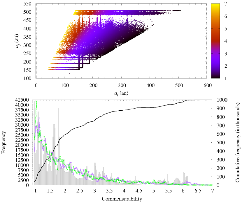
Figure 1: Commensurability map (top panel) for the values of the heliocentric semimajor axes and their uncertainties in Table 1. Frequency distribution (bottom panel) in $(a_{j}/a_{i})^{3/2}$ from the commensurability map. The results from a uniform spread in semimajor axis are plotted in purple and those from a biased uniform sample in green. The number of bins in the frequency distribution plot is 2 $n^{1/3}$, where $n$ is the number of pairs of virtual ETNOs tested, $n=10^{6}$. The black curve shows the cumulative distribution.

3.3 Barycentric orbits

Using the data in Table 2, we have obtained Fig. 2. As for the heliocentric orbits, there are significant deviations from the unperturbed scenario. Considering the values of the barycentric semimajor axes, the most obvious commensurabilities in Fig. 2 are 1.02, 1.11, 1.38, 1.65 and 1.71. Three of the statistically significant commensurabilities coincide with those found in the analysis of heliocentric orbits. In addition, several of these values are also present in the sequences associated with the main and trans-Neptunian belts. This is unlikely to be the result of chance alone.

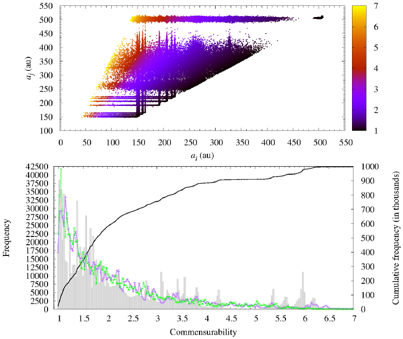
Figure 2: Same as Fig. 1 but for the barycentric values in Table 2.

4 Discussion

The analysis presented in the previous section shows that the frequency distribution of the ratio of orbital periods of known ETNOs is statistically incompatible with that of an unperturbed asteroid population following heliocentric/barycentric orbits. This result is unlikely to be a statistical artefact as the known ETNOs have been discovered by several independent surveys with, presumably, uncorrelated biases. If the frequency distribution of the ratio of periods is incompatible with an unperturbed scenario, how significant are the favoured commensurabilities? In order to answer this rather critical question, we have computed the difference between the frequency obtained from the observational values and that from the biased expectation (green curve in Figs 1 and 2) and divided by the value of the standard deviation in the biased case calculated as described above. Our results are plotted in Fig. 3. The number of statistically significant commensurabilities is larger than the few indicated above and found by simple visual inspection. The outcome is not dependent on the bin size; we have experimented with $n=10^{4}$ and $n=10^{5}$ and the results are fully consistent. The statistical significance analysis in Fig. 3 shows that our results are robust. Probabilistically speaking, there are simply too many ETNOs in commensurabilities compatible with the action of massive perturbers. Regarding the extremely significant value of the ratio of periods $\sim 6$ in Fig. 3, we would like to downplay this issue as two objects have values of the semimajor axis of $\sim 500$ au and several others have semimajor axes close to 150 au. These two values are the abrupt cutoffs in the distribution of semimajor axes.

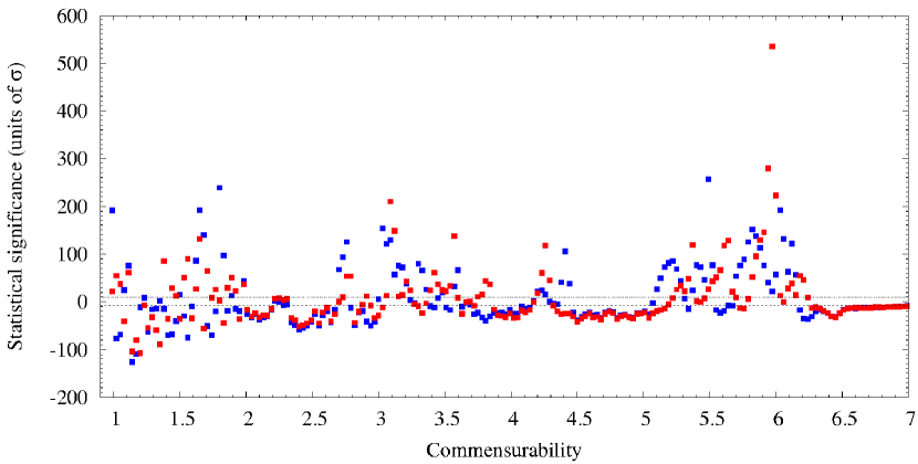
Figure 3: Statistical significance in terms of $\sigma$ of the deviations of the frequency distribution in the heliocentric (blue) and barycentric (red) cases (data from Figs 1 and 2) with respect to the biased expectations. The $\pm 9\sigma$ limits are also indicated.

One of the most surprising properties of the sample studied is the unusually large fraction of objects with ratio of periods $\sim 1$. This issue was already noticed in de la Fuente Marcos & de la Fuente Marcos (2014). In particular, the orbits of 2004 VN₁₁₂ and 2013 RF₉₈ are alike, and several objects have values of the barycentric semimajor axis within narrow ranges of each other. This could mean that some of these objects move co-orbital, i.e in a 1:1 mean motion resonance, with an unseen planet (or, more likely, several of them). Co-orbital motion is possible at high eccentricity (Namouni 1999; Namouni, Christou & Murray 1999; Namouni & Murray 2000). However, a more likely scenario is in the presence of higher order resonances like the 7:3 and 5:2 in the main asteroid belt that give a ratio of periods of 1.0699 or the 4:7 and 3:5 in the trans-Neptunian belt that give a ratio of 1.0501. Interior and exterior resonances are possible if there are multiple trans-Plutonian planets. Regarding the impact of this resonant scenario on the Planet Nine hypothesis, it is clearly compatible with it.

If the mechanisms responsible for inducing dynamical structure in the main and trans-Neptunian belts are also at work in the region occupied by the ETNOs then we should expect that for two given ETNOs in near commensurability:

$$\left(\frac{a_{\rm p}}{a_{j}}\right)^{3/2}\ \left(\frac{a_{i}}{a_{\rm p}}\right)^{3/2}=\left(\frac{m}{n}\right)\ \left(\frac{k}{l}\right)\,,$$ (1)

where $a_{\rm p}$ is the semimajor axis of the orbit of the perturber and $k,l,m,n$ are all small integers. This expression can be applied to two of the most clear clusterings in semimajor axis in Table 2. The average value of the barycentric semimajor axis of (90377) Sedna and 2007 TG₄₂₂ is 504 au. On the other hand, the equivalent mean value for 2004 VN₁₁₂, 2010 GB₁₇₄ and 2013 RF₉₈ is 332 au. These five objects are part of the set of six singled out by Batygin & Brown (2016). The associated period ratio for these two sets of ETNOs is 1.87. In the main asteroid belt, this ratio is obtained for objects trapped in the 5:3 mean motion resonance with Jupiter and those in the 3:1, that is one of the main resonances in the outer belt (Holman & Murray 1996). Making a dynamical analogy between the two situations and decomposing Eqn. 1 in two we have: $(a_{\rm p}/504)^{3/2}=5/3$ and $(332/a_{\rm p})^{3/2}=1/3$. The average of the two values of $a_{\rm p}$ is $\sim$700 au which is the favoured value for the semimajor axis of Planet Nine in Batygin & Brown (2016). The 1.8 commensurability has a statistical significance of 239$\sigma$ for heliocentric orbits, the 1.89 commensurability has 51$\sigma$ for barycentric orbits (see Fig. 3). This is unlikely to be mere coincidence.

Another example of the potential implications of our findings arises when we focus on 2003 HB₅₇, 2015 SO₂₀, 2005 RH₅₂, (445473) 2010 VZ₉₈ and 2013 GP₁₃₆, the first two could be in a 3:2 resonance with a hypothetical planet at $a=213$ au, with the other three in a 5:3 resonance with the same planet. In this framework, the pair 2003 HB₅₇ and 2015 SO₂₀ would be in a 10:9 accidental resonance with the other three ETNOs. A ratio of periods $\sim 1.1$ is present in both the main asteroid belt and the trans-Neptunian belt. The 1.1 commensurability has a statistical significance of 76$\sigma$ for heliocentric orbits and 61$\sigma$ for barycentric orbits (see Fig. 3). On the other hand, the 1.65 commensurability is present for both heliocentric (192$\sigma$) and barycentric (131$\sigma$) orbits; a similar analysis focusing on 2003 HB₅₇, 2013 GP₁₃₆, (82158) 2001 FP₁₈₅ and 2002 GB₃₂ is compatible with a hypothetical planet at $a=329$ au considering resonances (3/1)(5/9)=5/3$\sim$1.66. With the currently available data, degenerate solutions are possible, but they still hint at a multi-planet scenario. Trans-Plutonian planets may have been scattered out of the region of the giant planets early in the history of the Solar system (see e.g. Bromley & Kenyon 2014, 2016), but planets similar to Uranus or Neptune may also form at 125–750 au from the Sun (Kenyon & Bromley 2015, 2016).

5 Conclusions

In this Letter, we have explored the existence of commensurabilities between the known ETNOs. This analysis has been inspired by the hypothesis and discussion presented in Malhotra et al. (2016). Given the fact that these objects are not massive enough to induce orbit-orbit coupling by themselves, the existence of statistically significant commensurabilities could only signal the presence of massive unseen perturbers. Summarizing, our conclusions are as following.

• The clustering in orbital parameter space observed for the heliocentric orbits of the known ETNOs is also present when considering their barycentric orbits. In particular, $e$ clumps about 0.81$\pm$0.06, $i$ about 20°$\pm$8°, $\Omega$ about 134°$\pm$72°, and $\omega$ about $-$26°$\pm$49°. Statistical outliers do exist.

• The frequency distribution of the ratio of orbital periods of known ETNOs is statistically incompatible with that of an unperturbed asteroid population following heliocentric/barycentric orbits. In contrast, it resembles the ones present in the main and trans-Neptunian belts. The existence of statistically significant accidental commensurabilities between ETNOs strongly suggests that external perturbers induce the observed dynamical structure.

• The fraction of known ETNOs in 1:1 commensurabilities is dozens of times the expected value for a random population.

• A number of known ETNOs may be trapped in the 5:3 and 3:1 mean motion resonances with a putative Planet Nine with semimajor axis $\sim$700 au.

We must stress that our results are based on small number statistics, but it is also true that the deviations from what is expected for an unperturbed asteroid population following heliocentric/barycentric orbits are so strong that what is observed is unlikely to be the result of chance alone. Gravitational perturbations with sources in the region travelled by the ETNOs are the most probable explanation for the observed patterns.

References

- Batygin & Brown (2016) Batygin K., Brown M. E., 2016, AJ, 151, 22
- Box & Muller (1958) Box G. E. P., Muller M. E., 1958, Annals Math. Stat., 29, 610
- Bromley & Kenyon (2014) Bromley B. C., Kenyon S. J., 2014, ApJ, 796, 141
- Bromley & Kenyon (2016) Bromley B. C., Kenyon S. J., 2016, ApJ, submitted (arXiv:1603.08010)
- de la Fuente Marcos (2014) de la Fuente Marcos C., de la Fuente Marcos R., 2014, MNRAS, 443, L59
- de la Fuente Marcos (2016) de la Fuente Marcos C., de la Fuente Marcos R., 2016, MNRAS, 459, L66
- de la Fuente Marcos et al. (2015) de la Fuente Marcos C., de la Fuente Marcos R., Aarseth S. J., 2015, MNRAS, 446, 1867
- Gehrels (1986) Gehrels N., 1986, ApJ, 303, 336
- Giorgini (1996) Giorgini J. D. et al., 1996, BAAS, 28, 1158
- Gladman et al. (2012) Gladman B. et al., 2012, AJ, 144, 23
- Gomes et al. (2005) Gomes R. S., Gallardo T., Fernández J. A., Brunini A., 2005, Celest. Mech. Dyn. Astron., 91, 109
- Gomes et al. (2015) Gomes R. S., Soares J. S., Brasser R., 2015, Icarus, 258, 37
- Holman & Murray (1996) Holman M. J., Murray N. W., 1996, AJ, 112, 1278
- Kenyon & Bromley (2015) Kenyon S. J., Bromley B. C., 2015, ApJ, 806, 42
- Kenyon & Bromley (2016) Kenyon S. J., Bromley B. C., 2016, ApJ, submitted (arXiv:1603.08008)
- Malhotra et al. (2016) Malhotra R., Volk K., Wang X., 2016, ApJ, submitted (arXiv:1603.02196)
- Metropolis (1949) Metropolis N., Ulam S., 1949, J. Am. Stat. Assoc., 44, 335
- Murray & Dermott (1999) Murray C. D., Dermott S. F., 1999, Solar system Dynamics. Cambridge Univ. Press, Cambridge, p. 97
- Namouni (1999) Namouni F., 1999, Icarus, 137, 293
- Namouni & Murray (2000) Namouni F., Murray C. D., 2000, Celest. Mech. Dyn. Astron., 76, 131
- Namouni et al. (1999) Namouni F., Christou A. A., Murray C. D., 1999, Phys. Rev. Lett., 83, 2506
- Nesvorný & Morbidelli (1999) Nesvorný D., Morbidelli A., 1999, in Henrard J., Ferraz-Mello S., eds, Proc. IAU Colloq. 172, Impact of Modern Dynamics in Astronomy. Kluwer Academic Publishers, Dordrecht, p. 381
- Press (2007) Press W. H., Teukolsky S. A., Vetterling W. T., Flannery B. P., 2007, Numerical Recipes: The Art of Scientific Computing, 3rd edn. Cambridge Univ. Press, Cambridge
- Todorovic-Juchnicwicz (1981) Todorovic-Juchnicwicz B., 1981, Acta Astron., 31, 191
- Trujillo & Sheppard (2014) Trujillo C. A., Sheppard S. S., 2014, Nature, 507, 471