Distributed Entity Disambiguation with Per-Mention Learning

Abstract

Entity disambiguation, or mapping a phrase to its canonical representation in a knowledge base, is a fundamental step in many natural language processing applications. Existing techniques based on global ranking models fail to capture the individual peculiarities of the words and hence, either struggle to meet the accuracy requirements of many real-world applications or they are too complex to satisfy real-time constraints of applications.

In this paper, we propose a new disambiguation system that learns specialized features and models for disambiguating each ambiguous phrase in the English language. To train and validate the hundreds of thousands of learning models for this purpose, we use a Wikipedia hyperlink dataset with more than 170 million labelled annotations. We provide an extensive experimental evaluation to show that the accuracy of our approach compares favourably with respect to many state-of-the-art disambiguation systems. The training required for our approach can be easily distributed over a cluster. Furthermore, updating our system for new entities or calibrating it for special ones is a computationally fast process, that does not affect the disambiguation of the other entities.

1 Introduction

Many fundamental problems in natural language processing, such as text understanding, automatic summarization, semantic search, machine translation and linking information from heterogeneous sources, rely on entity disambiguation [7, 22]. The goal of entity disambiguation and more generally, word-sense disambiguation is to map potentially ambiguous words and phrases in the text to their canonical representation in an external knowledge base (e.g., Wikipedia, Freebase entries). This involves resolving the word ambiguities inherent to natural language, such as homonymy (phrases with multiple meanings) and synonymy (different phrases with similar meanings), thereby, revealing the underlying semantics of the text.

Challenges: This problem has been well-studied for well over a decade and has seen significant advances. However, existing disambiguation approaches still struggle to achieve the required accuracy-time trade-off for supporting real-world applications, particularly those that involve streaming text such as tweets, chats, emails, blogs and news articles.

A major reason behind the accuracy limitations of the existing approaches is that they rely on a single global ranking model (unsupervised or supervised) to map all entities. These approaches fail to capture the subtle nuances of individual words and phrases in the language. Even if dictionaries consider two words to be synonyms, the words often come from different origins, evoke different emotional images, differ in their general popularity and usage by demographic groups as well as how they relate to the local culture. Hence, even synonymous words can have very different probability distribution of being mapped to different nodes in the knowledge base. Global ranking models fail to capture the individuality of words and are, thus, more prone to mistakes in entity disambiguation.

In terms of running time, there are three aspects:

1. Training time: Ideally, it should be possible to break the training into a large number of small tasks for distributed scaling. Unfortunately, disambiguation approaches based on a global ranking model are either not amenable to parallelism at all or non-trivial to parallelize efficiently.

2. Query time: The real-time requirements of many applications constrain the extracted features to be light-weight and limits the complexity of the approaches. For instance, many joint disambiguation approaches are infeasible within real-time constraints.

3. Update time: Many applications require disambiguation systems to be continually updated as new words and phrases gain relevance (e.g., “Ebola crisis”, “Panama papers”, “Migrant crisis”) and additional training data becomes available. Ideally, extending a system for new phrases or calibrating it for special ones should be local operations, i.e., they should not affect the previous learning of other word phrases and they should be fast. Existing approaches based on global models (supervised or unsupervised) often require the computationally expensive operation of rebuilding the global model from scratch, every time there is an update.

Our Approach: In this paper, we propose a novel approach to address all of these issues in word-sense disambiguation. Our approach aims at learning the individual pecularities of entities (words and phrases) in the English language and learns a specialized classifier for each ambiguous phrase. This allows us to find and leverage features that best differentiate the different meanings of each entity.

To train the hundreds of thousands of classifiers for this purpose, we use the publicly available Wikipedia hyperlink dataset. This dataset contains more than 110 million annotations and we extend it by another 63 million annotations. Since the training of these classifiers is independent of each other, our approach can be easily parallelized and we use a distributed Spark cluster for this purpose. The features used in these classifiers are mostly based on text overlap and are, therefore, light-weight enough for its usage in real-time systems. Updating our system for new entities simply requires to learn the models for those entities - it is fast and does not affect the other classifiers. Also, our approach is more robust in the presence of noisy data. Furthermore, unlike the increasingly popular deep learning architectures, our approach is interpretable: it is easy to understand why our models chose a particular mapping for an entity. We provide an extensive experimental evaluation to show that the efficacy and accuracy of our approach compares favourably with respect to many state-of-the-art disambiguation systems.

Outline: The rest of the paper is organized as follows. Section 2 presents related disambiguation techniques. Section 3 gives a brief overview of the Wikipedia hyperlink data used in the training of our disambiguation system and describe a method to extend this annotation data. In Section 4, we present the details of our novel disambiguation approach. Section 5 describes the experiment set-up, comparison metrics, and also a method to scramble data sets for validation of different scenarios. Experiment results with different training settings on a part of Wikipedia data are in Section 6. Then, Section 7 shows our pruning method and results. Comparisons with Dbpedia Spotlight, TAGME and benchmarking results by the standard framework GERBIL are given in Section 8. Experiment results of full Wikipedia data and per-phrase accuracy are given in Section 9. Finally, we conclude this paper with some points for future works in Section 10.

2 Related Work

There is a substantial body of work focussing on the task of disambiguating entities to Wikipedia entries. The existing techniques can be roughly categorized into unsupervised approaches that are mostly graph-based and supervised approaches that learn a global ranking model for disambiguating all entities.

Graph-based unsupervised approaches: In these approaches, a weighted graph is generally constructed with two types of nodes: phrases (mention) from the text and the candidate entries (senses) for that phrase. For the mention-sense edges, the weights represent the likelihood of the sense for the mention in the text context such as those given by the overlapping metrics between the mention context and the sense context (Wikipedia article body). For the sense-sense edges, the weights capture their relatedness, e.g. the similarity between two Wikipedia articles in terms of categories, in-links, out-links. A scoring function is designed and then optimized on the target document so that a single sense is associated with one mention. Hoffart [12] solved the optimization by a dense subgraph algorithm; on the other hand, Han et al. [11] as well as Guo and Barbosa [9] used random walk on the graph and chose the candidate senses by the final state probability. Hulpus et al. [13] explored some path-based metrics for joint disambiguation. The AGDISTIS approach of Usbeck et al. [23] extracts a subgraph of DBpedia graph containing all the candidate senses and uses a centrality measure based on HITS algorithm on the extracted subgraph to score the senses. It then selects the sense with the highest authority score for each entity. Moro et al. [18] leveraged BabelNet to constructed a semantic graph in a different manner, where each node is a combination of mention and candidate sense. Thereafter, a densest subgraph is extracted and the senses with maximum scores are selected. Ganea et al. [8] consider a probabilistic graphical model (PBoH) that addresses collective entity disambiguation through the loopy belief propagation.

Since these graph-based solutions are mostly unsupervised, there is no parameter estimation or training during the design of the scoring function to guarantee the compatibility between the proposed scoring function and the observed errors in any trained data [11, 12, 20]. Some disambiguation systems do apply a training phase on the final scoring function (e.g., TAGME by Ferragina and Scaiella [6]), but even here, the learning is done with a global binary ranking classifier. An alternative system by Kulkarni et al. [14] uses a statistical graphical model where the unknown senses are treated as latent variables of a Markov random field. In this work, the relevance between mentions and senses is modelled by a node potential and trained with max-margin method. The trained potential is combined with a non-trained clique potential, representing the sense-sense relatedness, to form the final scoring function. However, maximizing this scoring function is NP-hard and computationally intensive [6].

Supervised global ranking models: On the other hand, non-graph-based solutions [4, 10, 15, 16, 17, 19] are mostly supervised in the linking phase. Milne and Witten [17] assumed that there exists unambiguous mentions associated with a single sense, and evaluated the relatedness between candidate senses and unambiguous mentions (senses). Then, a global ranking classifier is applied on the relatedness and commonness features. Not relying on the assumption of existing unambiguous mentions, Cucerzan [2] constructed document attribute vector as an attribute aggregation of all candidate senses and used scalar product to measure different similarity metrics between document and candidate senses. While the original method selected the best candidate by an unsupervised scoring function, it was later modified to use a global logistic regression model [3].

In [10], Han et al. proposed a generative probabilistic model, using the frequency of mentions and context words given a candidate sense, as independent generative features; this statistical model is also the core module of the public disambiguation service Dbpedia Spotlight [4]. Then, Olieman et al. proposed various adjustments (calibrating parameters, preprocessing text input, merging normal and capitalized results) to adapt Spotlight to both short and long texts [19]; Olieman et al. also used a global binary classifier with several similarity metrics to prune off uncertain Spotlight results.

In contrast to these approaches that learn a global ranking model for disambiguation, our approach learns specialized features and model for each mention. Furthermore, since the disambiguation learning is per-mention and the number of candidate senses is fixed per-mention, proper multi-class statistical model can be used instead of binary ranking classifier, and coherent predicted probability-across-class can be evaluated and used for subsequent analysis.

Per-mention disambiguation: In terms of per-mention disambiguation learning on the Wikipedia knowledge base, Qureshi et al.’s [21] method is the most similar to our proposed method. However, as their method only uses Wikipedia links and categories for feature design and is trained with a small Twitter annotation dataset (60 mentions), it does not fully leverage the rich and big Wikipedia annotation data to obtain highly accurate per-mention trained models. Also, while our feature extraction procedure is light and tuned to contrast different candidate senses per mention, their method extracts related categories, sub-categories and articles up to two depth level for each candidate sense, and requires pairwise relatedness scores between candidate sense and context senses. All these high cost features are computed on-the-fly due to the dependency on the context, potentially slowing down the disambiguation process.

Pruner: After the linking phase, most disambiguation systems use either binary classifiers or score thresholding to prune off uncertain annotations, trading off between precision and recall depending on the scenario [5, 10, 17, 20, 19]. As the recall values of our disambiguation are quite high, we focus on increasing precision to guarantee non-noisy disambiguation outputs for subsequent text analysis and applications. Both binary classifiers and thresholding are tested, as in previous methods. However, unlike these methods, our pruning is performed at per-mention and even per-candidate levels.

3 Annotation Data and Disambiguation Problem

For the notation purposes, from this section, the first encounters of new terms are marked by italic font, with their definitions provided in the corresponding places.

3.1 Data preprocessing

In this work, we use the publicly available Wikipedia dump 2015-07-29. This raw data is first processed by the script WikiExtractor, which removes XML metadata, templates, lists, unwanted namespaces, etc.

From the output data above, information for Wikipedia entities (articles) $e$ is extracted, including article ids ($e_{id}=e$), article titles ($e_{title}$), and text bodies ($e_{body}$).

In the text bodies of Wikipedia entities, there are hyperlink texts, linking text phrases to other Wikipedia entities. So, for the notation purposes, hyperlink texts are called annotations; their associated text phrases and Wikipedia entities are called mentions and senses accordingly .

Such annotations $a$, linking from mentions $m$ to Wikipedia senses $e$, contained in some Wikipedia articles $e^{\prime}$ are also extracted, with information of particular annotations such as the containing article ids ($a_{cid}=e^{\prime}_{id}=e^{\prime}$), the mentions ($a_{m}=m$), the destination senses ($a_{e}=e_{id}=e$) and the short texts around the annotations (annotation contexts $a_{context}$) . For the annotation contexts, a number of sentences are extracted from both sides of the annotation so that the number of words of combined sentences of each side exceeds a predefined context window value $n_{context}=50$ .

During this process, text elements such as text bodies $e_{body}$, mentions $a_{m}$, and annotation contexts $a_{context}$ are lemmatized using the python package nltk for the purpose of grouping different forms of the same term.

Disambiguation problem: The extracted labelled annotations are grouped by their mentions. Then, for a single unique mention $m$ such as “Java”, we obtain the list of unique associated senses from the annotation group of mention $m$, e.g. “Java (programming language)”, “Java coffee”, “Java Sea”, etc, and make them the candidate senses $e^{(i)}$ for mention $m$ with ($i=1,\ldots,|e|$ and $|e|$ is the number of candidate senses for mention $m$) . In the disambiguation problem, given a new unlabelled annotation $a^{\prime}$ with its mention $a^{\prime}_{m}=m$ and context $a^{\prime}_{context}$, one wants to find correct sense $a^{\prime}_{e}=e^{\star}$ among all candidate senses $e^{(i)}$.

3.2 Data extension

As data quantity is the key point in big data analysis in improving the performance of any learning algorithm, we want to enrich the annotation data as much as possible for the disambiguation problem. Noticing that most Wikipedia annotations are only applied for the first occurrence of text phrases and article self-links are not available, we extend the annotation data with the following extension procedure.

First, unique annotation pairs $(a_{m},a_{e})$ are extracted from each Wikipedia article $e^{\prime}$. If there is more than one annotation candidate article for a unique lemmatized mention $a_{m}$, the candidate article $e$ with the highest text overlapping between its title $e_{title}$ and annotation mention $a_{m}$ is selected. We also construct a unique self-annotation pair $(a_{m}=e^{\prime}_{title},a_{e}=e^{\prime})$ for each Wikipedia article $e^{\prime}$. This unique self-annotation pair takes precedence and overwrites any other pair of the same mention in $e^{\prime}$.

Next, the body of each Wikipedia article is scanned, where lemmatized unlinked text phrases that exactly match a mention $a_{m}$ from the set of unique annotation pairs are gathered and paired with the corresponding senses $a_{e}$. In this extended annotation dataset, original annotations are marked with extraction flags $a_{ef}=0$ while flags $1$ and $2$ are for annotations extended from original pairs and Wikipedia article titles, correspondingly.

There is one general case to be noted with the above procedure. For example, in the article $e^{(a)}_{title}=$ “Biomedical engineering”, there is an original annotation from $a^{(i)}_{m}=\text{``engineering''}$ to a more general article: $a^{(i)}_{e}=e^{(b)}$ with $e^{(b)}_{title}=\text{``Engineering''}$. Any unlinked text phrase “engineering” in that article is annotated to $a^{(j)}_{e}=e^{(b)}$ with $a^{(j)}_{ef}=1$, which may not be true. So, to deal with this issue, we remove the above annotations $a^{(j)}$ of flag $a^{(j)}_{ef}=1$ in this case.

Following this procedure, we are able to get around $63$ million additional annotations. The union of original and extended annotation datasets will be referred to as dataset $\mathcal{A}$ in the remainder of the paper. As Wikipedia is a highly coherent and formal dataset, manually edited by many people, we find the extended annotations to be of good quality.

The summary statistics of this data are given in Table 1; $\#\text{mentions}_{1}$ is the number of mentions that have exactly one candidate sense; $\#\text{mentions}_{>1}$ is for mentions with more than one candidate senses. In this paper, we target the disambiguation of $\text{mentions}_{>1}$.

Figure 1(a) shows the number of mentions of a particular number of candidate senses in log-log scale. While most mentions have only a few candidates, some of them such as “France”, “2010” can have more than $600$ candidate senses as they are used to refer to numerous specific entities and events in a year or a country, such as “French cinema”, “Rugby league in France”, “2010 America’s Cup”, “2010 in Ireland”, etc. Figure 1(b) shows the averaged number of annotations of mentions of a particular number of senses. This number is proportional to the training and validation size of the disambiguation learning per mention, discussed in later sections.

Table 1: Wikipedia summary statistics

$\#\text{main entities}$	4883834
$\#\text{redirection entities}$	6860485
$\#\text{mentions}_{1}$	8232340
$\#\text{mentions}_{>1}$	710044
$\#\text{original annotations}$	110003963
$\#\text{extended annotations}$	63375236
average context length	121.55

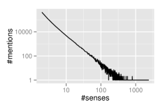
(a) $\#\text{mentions}$ vs $\#\text{senses}$

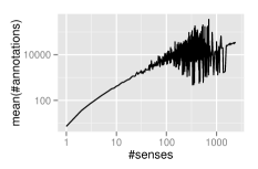
(b) mean(#annotations) vs $\#\text{senses}$

Figure 1: Summary statistics per sense

4 Disambiguation Method

With Wikipedia annotation data extracted and extended in the previous section, this section discusses the learning method and feature extraction for the disambiguation problem.

As briefly mentioned in Section 1, this paper uses a big data approach with supervised discriminative machine learning models for the disambiguation problem. Unlike methods where a single global supervised model is learned for all mentions [10, 19] or one global ranking model is applied on a varying number of candidate senses per encounter of mentions, [5, 6, 17], our disambiguation system learns and works on the basis of per lemmatized mention. Hence, annotations with the same lemmatized mention are grouped together for disambiguation learning. By doing so, the problem of disambiguating a particular mention becomes a formal problem of multi-class classification, which is, in our opinion, more statistically consistent and proper than a ranking binary classifier in selecting a candidate sense. .

From the machine learning and statistical inference perspective, this per-mention learning approach is like segmenting varying big data into small data bins of similar properties and then applying the learning on each data bin independently. Within each data bin (or mention), a model and features can be designed specifically for that particular mention. As multiple specialized predictors perform better than a global multi-purpose predictor, the performance of the disambiguation is improving.

4.1 Feature extraction

Most recent disambiguation works use commonness and relatedness features to rank a varying number of candidate senses of a particular mention [5, 6, 11, 17, 20]. Commonness features usually measure how common a sense is with respect to a mention, e.g. the probability that sense is used, given a particular mention. In our per-mention multi-class classification approach, all candidate-specific features that do not depend on the annotation context, including commonness, can be encapsulated in a single bias parameter for each class.

Relatedness, measuring the pairwise similarity between candidate senses of multiple mentions in same documents, is a very good coherence measurement of candidate senses. However, raletedness features heavily rely on the mention spotter, and have two possible shortcomings. Firstly, the spotter may fail to recognize a good number of potential mentions due to the informal and short data, such as tweets or chats. The lack of extracted mentions leads to a weak relatedness measurement and hence bad disambiguation. Secondly, a poorly trained spotter might return low quality mentions such as “yes” and “no”, while even a good spotter may result in redundant or noisy mentions. Contrary to the belief that more mentions is better for disambiguation, Piccinno showed that these noisy mentions can reduce the disambiguation accuracy [20] .

So, instead of using relatedness features, we decide to use the light-weight and robust word-based similarity features between annotation context and candidate sense context. We show that coupling the specialized per-mention classifier with these features, which are tuned to contrast candidate senses, can deliver a very accurate and fast disambiguation solution.

Usually, the similarity is measured by matching the annotation context directly to contexts of candidate senses such as the abstracts or the whole Wikipedia pages[14]. However, as the disambiguation is a per-mention classification, we can further tune candidate contexts to emphasize the contrast among candidates of a mention before evaluating the word-based similarity.

Specifically, for all unique candidate senses $e^{(i)}$ with $(i=1,\ldots,|e|)$ across the entire Wikipedia dataset of a particular mention $m$, we construct the tf-idf matrix, select and rank the top $n_{f;w}$ words by tf-idf values for each candidate, and put these ranked words into $n_{f;p}$ parts. As a result, for each candidate $e^{(i)}$, there are $n_{f;p}$ context parts $(c^{(e;i)}_{1},\ldots,c^{(e;i)}_{n_{f;p}})$; each part is a list of word-and-tfidf pairs $c^{(e;i)}_{j}=((w^{(e;i)}_{j,1},v^{(e;i)}_{j,1}),\ldots,(w^{(e;i)}_{j,\underline{n}_{f;w}},v^{(e;i)}_{j,\underline{n}_{f;w}}))$ where $w^{(e;\cdot)}_{\cdot,\cdot}$ is a ranked lemmatized word of an entity context, $v^{(e;\cdot)}_{\cdot,\cdot}$ is its corresponding tf-idf value and $\underline{n}_{f;w}=\lceil n_{f;w}/n_{f;p}\rceil$ is the number of words per part . Due to the properties of idf components, the above procedure results in the contrasting contexts of different candidate senses.

For an unlabelled annotation $a$, we transform its context $a_{context}$ to a list of words and counts $c^{(a)}=((w^{(a)}_{1},v^{(a)}_{1}),\ldots)$ where $w^{(a)}_{\cdot}$ is a unique word in the context $a_{context}$ and $v^{(a)}_{\cdot}$ is its occurrence count. The similarity between $a_{context}$ and a context part $c^{(e;i)}_{j}$ of a candidate sense $e^{(i)}$ are measured in four different ways:

$$sim_{wo}(a,c^{(e;i)}_{j}) =\frac{\sum_{k_{1},k_{2}}\mathbbm{I}(w^{(a)}_{k_{1}}=w^{(e;i)}_{j,k_{2}})}{\log(|a_{context}|+1)},$$

$$sim_{ws}(a,c^{(e;i)}_{j}) =\frac{\sum_{k_{1},k_{2}}v^{(a)}_{k_{1}}\mathbbm{I}(w^{(a)}_{k_{1}}=w^{(e;i)}_{j,k_{2}})}{\log(|a_{context}|+1)},$$

$$sim_{to}(a,c^{(e;i)}_{j}) =\frac{\sum_{k_{1},k_{2}}v^{(e;i)}_{j,k_{2}}\mathbbm{I}(w^{(a)}_{k_{1}}=w^{(e;i)}_{j,k_{2}})}{\log(|a_{context}|+1)},$$

$$sim_{ts}(a,c^{(e;i)}_{j}) =\frac{\sum_{k_{1},k_{2}}v^{(a)}_{k_{1}}v^{(e;i)}_{j,k_{2}}\mathbbm{I}(w^{(a)}_{k_{1}}=w^{(e;i)}_{j,k_{2}})}{\log(|a_{context}|+1)},$$

where $\mathbbm{I}(\cdot)$ is the indicator function and $|a_{context}|$ is the length of the annotation context, used for scaling different context length. So, the feature vector to disambiguate an annotation $a$ of mention $m=a_{m}$ is $r^{(a)}=(r^{(a)}_{1},\ldots,r^{(a)}_{n_{f;sim}})$, which is an aggregation of all above similarities of all candidates senses $e^{(i)}$; $n_{f;sim}=4n_{f;p}|e|$ is the total number of features.

4.2 Learning model

To perform per mention disambiguation, we use multinomial regression with the above similarity features, which is a statistically-proper classification model . Such a classification model can provide a consistent predicted class probability, which is useful for later pruning.

For a labelled annotation $a$ with mention $m$, observed senses $e$ and features $r^{(a)}_{k}$, the multinomial regression model can be defined as follows:

$$\mu^{(a)}_{i} =\alpha_{i,0}+\sum_{k}\alpha_{i,k}r^{(a)}_{k},$$

$$p^{(a)}_{i} =\frac{\exp(\mu^{(a)}_{i})}{\sum_{i^{\prime}}\exp(\mu^{(a)}_{i^{\prime}})},$$

$$e^{(a)} \sim p^{(a)}.$$

For the disambiguation of new annotations after the training phase, our method has the complexity $\mathcal{O}(|e|\times|a_{context}|)$ per-annotation. The system is highly scalable and all trained-model parameters, candidate senses, processing can be split by mentions evenly across different cluster nodes. The disambiguation process for any document can be parallelized on the annotation-level, which is important for real time processing of very long documents.

5 Experiment Set-up

5.1 System and implementation

One of the numerical challenges for this approach is the required computation power needed for the processing of more than 700K of unique ambiguous mentions and 170 million labelled annotations. Fortunately, as the feature construction and classification learning is per-mention, the disambiguation system is highly compatible with a data-parallel computation system. So, in order to deal with the numerical computation, we use Apache Spark, a distributed processing system based on Map-Reduce framework, for all data processing, feature extraction and model learning. As Spark supports distributed in-memory serialization, caching and parallel processing for big data with a simple but mature API, it satisfies our needs and provides a nice speed up. Hence, a Spark cluster is set up for this disambiguation system, consisting three 16$\times$2.6GHz 96GB-RAM machines.

All the algorithms and procedures are implemented in Python with PySpark API. For machine learning methods, we use the standard open source library scikit-learn. Even though the code is not highly optimized like a C/C++ implementation, it is shown later that the system perform disambiguation in about 2.8ms per annotation.

5.2 Training and validation set-up

For the purposes of training and validation, the annotation dataset $\mathcal{A}$ in Section 3 is split by ratio (90%,10%) per-mention. The 90% training dataset is denoted by $\mathcal{A}_{1}$ and the other is by $\mathcal{A}_{2}$. In order to validate the disambiguation system in different data scenarios such as short-text and noisy-text, we use the following transformation on the original annotation dataset and create different datasets.

For a mention $m$ and candidate senses $e^{(i)}$ $(i=1,\ldots,|e|)$, a random noisy vocabulary $\mathcal{V}_{m}$ of unique words is first constructed by doing set-union on words of $e^{(i)}_{body}$. Then for every annotation $a$ of mentions $m$, a new annotation context $a^{\prime}_{context}$ is formed by sampling-without-replacement $n_{s,1}=p_{s,1}\times|a_{context}|$ words from $a_{context}$ and $n_{s,2}=p_{s,2}\times|a_{context}|$ words from $\mathcal{V}_{m}$. All new annotations $a^{\prime}$ with contexts $a^{\prime}_{context}$ form a new dataset. Parameter $p_{s,1}\leq 1$ is the shrinkage factor of the transformation while parameter $p_{s,2}$ implies the noise level from other candidate senses.

Four such datasets are constructed with parameters $p_{s,1}$, $p_{s,2}$ specified in Table 2 and are only used for validation purpose. Notice that any n-gram mentions ($n\geq 2$) of the original annotation context can be broken by the sampling operation. Our disambiguation system, by design, is robust with respect to such scrambled contexts while relatedness-based methods would suffer from this added noise.

Table 2: Data transformation parameters

Dataset	$\mathcal{B}$	$\mathcal{C}$	$\mathcal{D}$	$\mathcal{E}$
$p_{s,1}$	80%	60%	40%	20%
$p_{s,2}$	20%	0%	0%	0%

5.3 Metrics

For comparison purpose, we use the following precision and recall definitions:

$$\mathcal{P} =\frac{\sum_{d_{i},a\in d_{i},\widetilde{a}\in d_{i}}\mathbbm{I}(a=\widetilde{a},a_{e}=\widetilde{a}_{e})}{\sum_{d_{i},\widetilde{a}\in d_{i}}1},$$

$$\mathcal{R} =\frac{\sum_{d_{i},a\in d_{i},\widetilde{a}\in d_{i}}\mathbbm{I}(a=\widetilde{a},a_{e}=\widetilde{a}_{e})}{\sum_{d_{i},a\in d_{i}}1},$$

where $d_{i}$ is a document; $a$ and $\widetilde{a}$ are ground-truth annotation and predicted annotations, correspondingly . These definitions are equivalent to the comparison metrics in the long term track in ERD-2014’s challenge [1].

The definitions of precision and recall above may be biased to mentions with a large number of labelled annotations in Wikipedia dataset. Hence, we also use the following average precision-recall across mentions:

$$\underline{\mathcal{P}} =\frac{\sum_{m}P_{m}}{|m|},$$

$$\underline{\mathcal{R}} =\frac{\sum_{m}R_{m}}{|m|},$$

where $|m|$ is the number of unique mentions; $P_{m}$ and $R_{m}$ are precision and recall of a specific mention $m$.

6 Analysis on Learning Settings

In this section, we explore and analyze the accuracy of the proposed disambiguation system by varying several configurable variables.

In the feature extraction step, $n_{f;w}$ defines the number of unique words, ranked by tfidf values, in each candidate sense context, used for matching with an annotation context. In the case of using a large value of $n_{f;w}$, we may expect the effect of high ranking words to the disambiguation classifier is different from ones of low ranking words, and hence divide them in a number of parts $n_{f;p}$, as described in Section 4.1. In terms of computation, $n_{f;w}$ affects the cost of matching the annotation context with the top-ranked words of candidate context while $n_{f;p}$ affects the number of training features.

Another variable that affects the system performance is the classifier. So, aside from multinomial regression, we also evaluate the accuracy results with one-versus-the-rest logistic regression, random forest and support vector classification.

For this analysis of configurable system variables, the system is trained and evaluated on 8834 random unique mentions; also in any dataset, if there are more than $5000$ annotations of a specific candidate sense of a mention, we sample-without-replacement $5000$ annotations for that pair of mention-sense to reduce the experiment running time . The validation results are provided for both the original validation dataset $\mathcal{A}_{2}$ and the scrambled datasets in Section 5.2.

Table 3: Performance results of different settings $(n_{f;w},n_{f;p})$ with multinomial regression. The best results are in bold.

$n_{f;w}$ $n_{f;p}$ $\mathcal{P}^{\mathcal{A}_{2}}$ $\underline{\mathcal{P}}^{\mathcal{A}_{2}}$ $\mathcal{P}^{\mathcal{B}}$ $\underline{\mathcal{P}}^{\mathcal{B}}$ $\mathcal{P}^{\mathcal{C}}$ $\underline{\mathcal{P}}^{\mathcal{C}}$ $\mathcal{P}^{\mathcal{D}}$ $\underline{\mathcal{P}}^{\mathcal{D}}$ $\mathcal{P}^{\mathcal{E}}$ $\underline{\mathcal{P}}^{\mathcal{E}}$ $\mathcal{T}_{\text{total}}$ $\mathcal{T}_{\text{pred}}$ $(\times 10^{3}\text{s})$ $(\text{ms})$ 400 8 .9186 .9206 .9325 .9274 .9351 .9529 .9053 .9260 .8550 .8787 47.56 5.69 300 6 .9182 .9199 .9315 .9266 .9331 .9504 .9031 .9231 .8536 .8771 39.18 4.89 200 4 .9174 .9200 .9297 .9248 .9298 .9458 .9005 .9183 .8524 .8744 29.66 3.95 100 2 .9157 .9163 .9243 .9203 .9225 .9347 .8947 .9098 .8487 .8686 2.55 3.00 400 1 .9152 .9215 .9213 .9186 .9182 .9296 .8951 .9106 .8532 .8754 24.32 3.91 300 1 .9150 .9211 .9212 .9181 .9181 .9292 .8949 .9104 .8530 .8751 22.74 3.61 200 1 .9147 .9203 .9208 .9175 .9174 .9286 .8940 .9095 .8518 .8740 2.71 3.33 100 1 .9138 .9188 .9193 .9163 .9160 .9263 .8916 .9063 .8491 .8701 18.13 2.81

First, performance results by varying $n_{f;w}$ and $n_{f;p}$ with multinomial regression are given in Table 3. $\mathcal{T}_{\text{total}}$ is the total time of feature construction, training and validation of all datasets and $\mathcal{T}_{\text{pred}}$ is the prediction time per-annotation (including the feature construction time); both are measured in a sequential manner as the running time of all mentions in all Spark executor instances is summed up before the evaluation.

As we want to validate purely the disambiguation process, we do not prune off uncertain predictions in this section and the disambiguation always returns a non-NIL candidate for any annotation. Consequently, precision, recall and F-measure are all equal and only precision values are reported.

We make the following observations about Table 3:

• Increasing $n_{f;w}$ and $n_{f;p}$ raises the precision but the increment magnitude is diminishing.

• There is a trade off between precision and running time/prediction time. The more the number of top-ranked candidate context words and the number of features, the higher the precision but the slower the disambiguation process and the longer the prediction time per-annotation.

• As expected, the precision decreases when the annotation context becomes smaller and smaller from validation dataset $\mathcal{C}$ to $\mathcal{E}$.

• Between dataset $\mathcal{B}$ and $\mathcal{C}$, $\mathcal{B}$ has longer but noisier context than $\mathcal{C}$, resulting in a lower precision.

• Mention-average precision $\underline{\mathcal{P}}$ is higher than the standard precision $\mathcal{P}$, in general, implying that mentions with higher number of labelled annotations have lower per-mention precision. Notice that these mentions also have a much higher number of candidate senses, as shown in Figure 1(b).

The comparison between different classifiers is shown in Table 4. For this problem, in terms of precision, multinomial regression (MR) and one-versus-the-rest logistic regression (LR) seem to be clear winners. However, LR and also support vector classifier (SVC) have very long training time and hence total time, which is a big disadvantage when the disambiguation training is applied on the full Wikipedia dataset. Accuracy results of random forest with 10 estimators (RF-10) or 30 estimators (RF-30) are not as high as the others. Hence, MR seems to be a better choice for this task, especially when it is statistically proper and can provide the coherent prediction probability across candidate classes for the pruner described in the next section.

Table 4: Performance results of different classifiers (CLS) on two settings of $(n_{f;w},n_{f;p})$. The best results in each setting are in bold.

$(n_{f;w},$ CLS $\mathcal{P}^{\mathcal{A}_{2}}$ $\underline{\mathcal{P}}^{\mathcal{A}_{2}}$ $\mathcal{P}^{\mathcal{B}}$ $\underline{\mathcal{P}}^{\mathcal{B}}$ $\mathcal{P}^{\mathcal{C}}$ $\underline{\mathcal{P}}^{\mathcal{C}}$ $\mathcal{P}^{\mathcal{D}}$ $\underline{\mathcal{P}}^{\mathcal{D}}$ $\mathcal{P}^{\mathcal{E}}$ $\underline{\mathcal{P}}^{\mathcal{E}}$ $\mathcal{T}_{\text{total}}$ $\mathcal{T}_{\text{pred}}$  $n_{f;p})$ $(\times 10^{3}\text{s})$ $(\text{ms})$ (400,8) SVC .9019 .8185 .9237 .9029 .9269 .9375 .8935 .9037 .8397 .8495 228.46 5.85 MR .9186 .9206 .9325 .9274 .9351 .9529 .9053 .9260 .8550 .8787 47.56 5.69 LR .9127 .8147 .9350 .9091 .9362 .9389 .9091 .9115 .8610 .8644 252.24 5.70 RF-10 .8938 .9165 .8889 .8838 .8828 .9060 .8563 .8784 .8223 .8406 33.45 5.57 RF-30 .9052 .9293 .9039 .9004 .8972 .9217 .8709 .8939 .8368 .8535 35.15 5.70 (100,1) SVC .9091 .8979 .9166 .9164 .9140 .9286 .8878 .9030 .8422 .8595 31.35 2.86 MR .9138 .9188 .9193 .9163 .9160 .9263 .8916 .9063 .8491 .8701 18.13 2.81 LR .9140 .9002 .9185 .9111 .9154 .9207 .8947 .9015 .8560 .8658 43.41 2.78 RF-10 .8989 .9118 .8966 .8921 .8884 .9042 .8632 .8802 .8288 .8431 15.71 2.80 RF-30 .9080 .9208 .9089 .9036 .9001 .9164 .8746 .8905 .8402 .8542 16.65 2.85

7 Pruner

In the previous section, for a pure analysis of disambiguation accuracy, the system is forced to return one candidate sense for any annotation. In this section, we propose two approaches to prune off uncertain annotation and explore the trade off between precision and recall. These pruners are hence natural solutions for NIL-detection problem.

7.1 Pruning with binary classifiers

Similar to other proposed pruning solutions [5, 19, 20] we also consider a binary classifier to prune off uncertain results from the previous disambiguation phase in Section 4. However, instead of using a single global classifier, we faithfully follow a per-mention learning approach and use a different binary classifier for each unique mention.

For any target ground-truth annotation $a$ of a unique mention $m$, a predicted annotation $\widetilde{a}$ is returned by the disambiguation. To learn the pruner of mention $m$, three features are first evaluated for each $\widetilde{a}$: $g^{(\widetilde{a})}_{1}$ is the predicted probability of multinomial classifier of $\widetilde{a}$; $g^{(\widetilde{a})}_{2}$ is the longest-common-string length between $m$ and the predicted sense title $\widetilde{e}_{title}$ ($\widetilde{e}=\widetilde{a}_{e}$); $g^{(\widetilde{a})}_{3}$ is another string-overlapping metric, defined by the ratio $\frac{m\cap\widetilde{e}_{title}}{m\cup\widetilde{e}_{title}}$. Both the length $g^{(\widetilde{a})}_{2}$ and the union, intersection operators are measured on the word-level, not character-level; disambiguation parts in Wikipedia title, e.g. the part ”(language)” in ”Java_(language)”, are removed before the intersection and union evaluation. The objective of this pruner is to learn the binary label $\mathbbm{I}(a_{e}=\widetilde{a}_{e})$ of a particular mention $m$. Any new predicted annotation $\widetilde{a}^{\prime}$ is removed if its predicted binary pruning label is negative.

In order to avoid validation bias, we first employ the same technique in Section 5.2 to create a new dataset $\mathcal{F}$ with a non-zero $p^{(\mathcal{F})}_{s,1}$ (noise is not considered for this dataset: $p^{(\mathcal{F})}_{s,2}=0$) and then train a binary classifier with $\mathcal{F}$. Finally, the trained classifiers are applied on the disambiguation results of other validation datasets such as $\mathcal{A}_{2}$, $\mathcal{B}$, etc.

We further extend the pruning analysis by using a binary classifier on each candidate of a mention. In this case, features $g^{(\widetilde{a})}_{2:3}$ are dropped as they are mathematically equivalent to a single per-candidate bias parameter.

The pruning results for both approaches are shown in Table 5: the classifier used for these experiments is random forest with 30 estimators; $p^{(\mathcal{F})}_{s,1}$ is set to 80%. $\mathcal{P}$ is the precision (the same as recall and F-measure) before pruning while $\mathcal{P}_{\text{pr}}$, $\mathcal{R}_{\text{pr}}$, $\mathcal{F}_{\text{pr}}$ are the precision, recall, F-measure after pruning. From the table, it can be seen that the precision can be pushed up to 0.5%-1.0% higher, with the penalty of recall (decreased by 2.8%-3.0%); also, the difference between per-mention and per-candidate classifiers is negligible. The pruning effect by using a binary classifier on setting $(n_{f;w}=\text{100},\allowbreak n_{f;p}=\text{1})$ is a little bit stronger than on $(n_{f;w}=\text{400},\allowbreak n_{f;p}=\text{8})$: higher precision (increased by 0.7%-1.3%) but lower recall (decreased by 4.3%-4.7%)

We also conduct other pruning experiments using logistic regression instead of random forest. However, it has a very little pruning effect (all metrics only vary about 0.2%-0.3%), implying a similar classification effect between the disambiguation classifier MR and the pruner classifier LR.

Table 5: Precision-recall trade-off results with binary classifiers

$n_{f;w}$ $n_{f;p}$ Pruner Metric Dataset type $\mathcal{A}_{2}$ $\mathcal{B}$ $\mathcal{C}$ $\mathcal{D}$ $\mathcal{E}$ 400 8 $\mathcal{P}$ .9186 .9325 .9351 .9053 .8550 per-mention $\mathcal{P}_{\text{pr}}$ .9267 .9379 .9404 .9119 .8623 $\mathcal{R}_{\text{pr}}$ .8897 .9028 .9054 .8760 .8265 $\mathcal{F}_{\text{pr}}$ .9079 .9200 .9226 .8936 .8440 per-candidate $\mathcal{P}_{\text{pr}}$ .9288 .9386 .9412 .9127 .8634 $\mathcal{R}_{\text{pr}}$ .8901 .9024 .9054 .8759 .8267 $\mathcal{F}_{\text{pr}}$ .9091 .9202 .9229 .8939 .8446 100 1 $\mathcal{P}$ .9138 .9193 .9160 .8916 .8491 per-mention $\mathcal{P}_{\text{pr}}$ .9238 .9269 .9240 .9000 .8573 $\mathcal{R}_{\text{pr}}$ .8702 .8727 .8700 .8465 .8064 $\mathcal{F}_{\text{pr}}$ .8962 .8990 .8962 .8724 .8311 per-candidate $\mathcal{P}_{\text{pr}}$ .9266 .9276 .9248 .9007 .8580 $\mathcal{R}_{\text{pr}}$ .8696 .8727 .8703 .8472 .8066 $\mathcal{F}_{\text{pr}}$ .8972 .8993 .8967 .8731 .8315

7.2 Thresholding predicted probability

A binary classifier in the previous section is a nice and automatic pruner. However, in some cases, we still want to increase the pruning strength, pushing precision even higher at the cost of recall; hence, in this section, we use a method to adjust the lower threshold of the predicted probability: only predicted annotation with $g^{(\widetilde{a})}_{1}$ higher than the threshold is kept by the system. Instead of using a global lower threshold value, we find one threshold value for each candidate of a mention, satisfying a global predefined condition of F-measure and precision.

The adjustment is trained with dataset $\mathcal{F}$ as in the previous section. For each mention, all predicted annotations are grouped accordingly to their predicted senses $\widetilde{e}$ and then Algorithm 1 is applied on each group independently. Finally, the estimated thresholds are used to prune off uncertain annotations in the other datasets such as $\mathcal{A}_{2}$, $\mathcal{B}$, etc.

The pruning results of Algorithm 1 are shown in Table 6. From both the algorithm and the results, it can be seen that the lower the control parameters $\beta_{0}$, $\beta_{1}$, the looser the condition and the higher the potential precision value. The procedure consistently increases the precision values by 1.1%-2.8% across different settings and datasets, illustrating a stronger pruning effect than using binary classifiers.

In conclusion for this section, we believe pruning is very important as it increases the precision and provides non-noisy disambiguation results needed for subsequent text analysis such as summarization or similarity measurement. It is especially true in our system as the recall value is quite high and we can extract enough information from the ground truth.

1

Input: Predicted annotations $\widetilde{a}^{(j)}$ ($j=1\ldots J$) of the same predicted sense $\widetilde{e}$

         Each annotation $\widetilde{a}^{(j)}$ is associated with a predicted probability $g^{(j)}=g^{(\widetilde{a}^{(j)})}_{1}$ and a binary label $h^{(j)}$ ($h^{(j)}=1$ if $\widetilde{a}^{(j)}$ is a correct annotation)

         Control parameters $\beta_{0}$ and $\beta_{1}$

2

3Calculate the precision $p^{\prime}$ and F-measure $f^{\prime}$ when there is no pruning threshold, using labels $h^{(j)}$.

4Calculate the precision $p^{(j)}$, F-measure $f^{(j)}$ at all threshold values $g^{(j)}$.

5Find the index set $\mathcal{S}=\{k:(f^{(k)}-f^{\prime})\geq\beta_{0},\text{and }(p^{(k)}-p^{\prime}+f^{(k)}-f^{\prime})\geq\beta_{1}\}$.

6If $\mathcal{S}$ not empty, find $k^{\prime}=\operatorname{argmax}_{k\in\mathcal{S}}(p^{(k)})$. Otherwise, find $k^{\prime}=\operatorname{argmax}_{j=1\ldots J}(f^{(j)},p^{(j)})$.

Return $g^{(k^{\prime})}$ as the target threshold.

Algorithm 1 Per-candidate threshold adjustment

Table 6: Precision-recall trade-off results with per-candidate threshold adjustment

$n_{f;w}$ $n_{f;p}$ $\beta_{0}$ $\beta_{1}$ Metric Dataset $\mathcal{A}_{2}$ $\mathcal{B}$ $\mathcal{C}$ $\mathcal{D}$ $\mathcal{E}$ 400 8 $\mathcal{P}$ .9186 .9325 .9351 .9053 .8550 -0.05 -0.02 $\mathcal{P}_{\text{pr}}$ .9327 .9439 .9472 .9206 .8735 $\mathcal{R}_{\text{pr}}$ .8911 .9022 .9058 .8735 .8205 $\mathcal{F}_{\text{pr}}$ .9114 .9226 .9261 .8964 .8462 -0.15 -0.05 $\mathcal{P}_{\text{pr}}$ .9374 .9479 .9512 .9257 .8802 $\mathcal{R}_{\text{pr}}$ .8691 .8780 .8820 .8498 .7974 $\mathcal{F}_{\text{pr}}$ .9019 .9116 .9153 .8861 .8367 100 1 $\mathcal{P}$ .9138 .9193 .9160 .8916 .8491 -0.05 -0.02 $\mathcal{P}_{\text{pr}}$ .9301 .9343 .9321 .9095 .8690 $\mathcal{R}_{\text{pr}}$ .8769 .8777 .8763 .8499 .8058 $\mathcal{F}_{\text{pr}}$ .9027 .9051 .9033 .8787 .8362 -0.15 -0.05 $\mathcal{P}_{\text{pr}}$ .9358 .9399 .9377 .9162 .8766 $\mathcal{R}_{\text{pr}}$ .8448 .8427 .8423 .8160 .7734 $\mathcal{F}_{\text{pr}}$ .8879 .8886 .8875 .8632 .8218

8 Comparison to Other Systems

Table 7: Comparison of Dbpedia Spotlight (DS) and our proposed system (PML)

DS instance $|{\mathcal{G}^{\prime}}|$ $\mathcal{P}_{DS}$ $\underline{\mathcal{P}}_{DS}$ $\mathcal{P}_{PML}$ $\underline{\mathcal{P}}_{PML}$ ($\gamma$) 0.0 65109 .8781 .8169 .9035 .8985 0.5 64586 .8822 .8201 .9051 .8989

Table 8: Comparison of TagMe (TM) and our proposed system (PML)

$|{\mathcal{G}^{\prime}}|$ $\mathcal{P}_{TM}$ $\underline{\mathcal{P}}_{TM}$ $\mathcal{P}_{PML}$ $\underline{\mathcal{P}}_{PML}$ 37872 .8752 .8244 .9077 .8950

Table 9: GERBIL comparison of different systems. The micro-F1 (top) and macro-F1 (bottom) scores of each system on each dataset are reported. Each column displays the best micro/macro-F1 score in red (marking the row with $\dagger$), and the second best micro/macro-F1 score in blue (marking the row with $\ddagger$).

	Datasets
	ACE2004	AIDA-CoNLL	AQUAINT	DBSpotlight	IITB	KORE50	Micropost	MSNBC	N3-Reuters-128	N3-RSS-500	OKE-2015
PML	.637	$\ddagger$.545	.685	$\dagger$.806	.460	.403	.527	.573	$\ddagger$.553	$\dagger$.677	.737
	$\dagger$.793	$\ddagger$.571	.683	$\dagger$.812	$\ddagger$.459	.376	.729	$\dagger$.648	$\ddagger$.592	$\dagger$.676	.742
AGDISTIS	.618	.498	.508	.263	$\ddagger$.467	.323	.323	$\ddagger$.621	$\dagger$.642	$\ddagger$.607	.615
	.752	.491	.495	.273	$\dagger$.480	.290	.593	.569	$\dagger$.699	$\ddagger$.607	.629
AIDA	.076	.416	.071	.210	.166	$\ddagger$.623	.331	.069	.353	.404	.617
	.410	.384	.072	.184	.173	$\ddagger$.563	.556	.077	.294	.347	.607
Babelfy	.517	.543	.668	.520	.364	$\dagger$.731	.471	.600	.439	.441	.684
	.685	.496	.667	.512	.348	$\dagger$.696	.621	.538	.378	.379	.663
DBSpotlight	.471	.426	.520	.701	.296	.439	.495	.351	.325	.200	.244
	.664	.436	.502	.675	.279	.401	.660	.333	.255	.161	.200
Dexter	.507	.407	.513	.284	.204	.183	.404	.293	.354	.369	.580
	.667	.387	.502	.251	.204	.123	.587	.298	.302	.293	.510
EC-NER	.488	.439	.403	.244	.137	.290	.412	.429	.365	.331	.192
	.656	.420	.369	.194	.150	.252	.594	.407	.335	.320	.160
Kea	.634	.539	$\dagger$.763	$\ddagger$.733	$\dagger$.472	.588	$\dagger$.631	$\dagger$.662	.501	.435	$\ddagger$.761
	.755	.524	$\dagger$.753	$\ddagger$.725	.453	.527	$\dagger$.758	$\ddagger$.615	.447	.387	$\ddagger$.753
NERD-ML	.558	.465	.575	.548	.422	.312	.478	.513	.402	.367	.740
	.714	.427	.554	.528	.411	.252	.629	.502	.340	.297	.719
TagMe 2	$\dagger$.660	.513	$\ddagger$.723	.661	.385	.590	.578	.590	.445	.470	$\dagger$.832
	$\ddagger$.776	.481	.708	.642	.372	.532	.712	.556	.380	.391	$\dagger$.814
WAT	$\ddagger$.643	$\dagger$.597	.714	.653	.401	.593	$\ddagger$.601	.601	.504	.433	.697
	.758	$\dagger$.581	$\ddagger$.714	.666	.385	.491	$\ddagger$.740	.542	.427	.364	.648

For the remainder of the paper we refer to the per-mention learning disambiguation system described above as PML, for brevity.

8.1 Comparison with Wikipedia as Ground Truth

In this section, we compare the proposed disambiguation system with Dbpedia Spotlight and TagMe. In the experiment, we only used ground truth annotations from dataset $\mathcal{A}_{2}$; for fairness we do not use any annotations created by extending the data.

An annotation set $\mathcal{G}\subset\mathcal{A}_{2}$ is used as an input of two Spotlight instances of different confidence values $\gamma=0.0$ and $\gamma=0.5$. We note that as Spotlight may not return disambiguation results for intended target mentions in annotations input due to pruning, Spotlight outputs are only for a subset $\mathcal{G}^{\prime}\subset\mathcal{G}$. We then use the proposed PML disambiguation system of setting $(n_{f;w}=100,n_{f;p}=1)$ without pruning on $\mathcal{G}^{\prime}$. The precision results are shown in Table 7, indicating that our proposed system has a higher accuracy of between 2.2% and 8.2% depending on the metric. The precision drop from $\mathcal{P}_{DS}$ to $\underline{\mathcal{P}}_{DS}$ implies that Spotlight disambiguation does not work as well as PML across distinct mentions.

For TagMe, a similar methodology is employed, but with a minor difference: the TagMe web API does not allow the user to specify the annotation for disambiguation. As a result, we rely on the TagMe spotter, and only include results where TagMe annotated exactly the same mention as the ground truth data. The precision results are shown in Table 8, indicating that our proposed system has a higher accuracy from 3.3% to 7.1%.

8.2 Comparison using GERBIL

To provide convincing evidence that our system works well on more than just Wikipedia text, we also compared our system to $10$ other disambiguation systems over $11$ different datasets. This was done by implementing a web-based API for our system that is compatible with GERBIL 1.2.2. [24]. We refer the interested reader to the GERBIL website and paper [24] for a complete description of these systems and datasets. The task we considered the strong annotation task (D2KB). In this task we are given an input text containing a number of marked phrases, and must return the entity our system associates with each marked phrase.

In order to produce a fair comparison, we made made two additions to our system for this test. The first is a preprocessing step in which we examine the phrase to be annotated and prune it (returning NIL) if it comes from a list of stop words (common verbs). Secondly, if no classifier is found for the phrase to be annotated, we examine the list of DBPedia transitive redirects for the phrase. If the phrase appears as a redirect, we return the corresponding entity associated with the redirect.

We tested our system using all datasets available by default in GERBIL, which are primarily based on news articles, RSS feeds, and tweets. In Table 9 we report, for each combination of system and dataset, the micro-F1 (top) and macro-F1 (bottom) scores. The micro-F1 score is the F1-measure aggregated across annotations, while the macro-F1 score is aggregated across documents.

Firstly, we observe that even though our system does not perform any coherence pruning, it consistently achieves very high macro-F1 scores. In fact, these macro-F1 scores are the highest in terms of average, $.644$, and lowest in terms of rank-average, $2.45$; Kea comes in second with $.609$ and $2.64$ respectively. In terms of micro-F1, we fall slightly short of Kea in terms of average and rank-average, $.611$ vs. $.600$ and $2.72$ vs. $3.36$, respectively.

Secondly, our system does extremely well on news. If we restrict ourselves to the news datasets (ACE2004, AIDA/CoNLL, AQUAINT, MSNBC, N3-Reuters-128, N3-RSS-500), then we achieve the highest average and lowest rank-average scores in terms of both micro-F1 and macro-F1: $.661$/$1.83$ and $.612$/$3$.

Thirdly, our system however performs quite poorly on the KORE50 dataset. Many entries in this dataset are single sentences involving very ambiguous entities: since our system does not perform joint disambiguation, these highly ambiguous entities are problematic. For example, one of the documents in the KORE50 dataset is, “David and Victoria added spice to their marriage.”, where the underlined phrases are to be disambiguated. The correct entities are “David Beckham” and “Victoria Beckham”, respectively, whereas PML returns the entities “David”, and “Victoria Song”. The first entity is returned due to bias towards in the absense of context, whereas the second result is a performer who appeared in a Korean reality TV show called “We got Married”.

We also note that there are systems not currently available to test through GERBIL that nonetheless have published similar comparisons. One issue however is that these comparisons are made using older versions of GERBIL, and that several changes have been made to recent versions of the system that drastically change these performance numbers. For this reason, we cannot directly compare our system to other recent systems such as that of Ganea et al. [8], since their published comparison uses a different version of GERBIL.

9 Full-data Experiment

In this section, the disambiguation experiment is extended to all Wikipedia mentions of more than one candidate senses. Due to the long processing time of more than 170 million annotations, we only run the system with one setting $(n_{f;w}=100,n_{f;p}=1)$ using multinomial regression. Also, as in Section 6, in any dataset, if a candidate sense has more than $5000$ labelled annotations, we sample-without-replacement $5000$ of these annotations to reduce the training and validation time. The precision results and time statistics are presented in Table 10 and it can be seen that the full performance results are stable and comparable to the ones of the corresponding setting in Table 3.

Aside from the global precision, another interesting aspect for this method is the performance of each unique mention. So, in this regard, per-mention precisions for all mentions are evaluated, smoothed and plotted against the number of candidate senses of mentions for all datasets in Figure 2. Results for dataset $\mathcal{A}_{2}$ have wider quantile ranges as its size is only about $10\%$ of the other datasets’. As expected, when the number of candidate senses of a mention increases, the disambiguation becomes more difficult and the precision reduces. From Figure 2(c) to Figure 2(e), the proportional effect of target context size $|a_{context}|$ to per-mention precision can be clearly seen, which is especially strong with respect to mentions of high number of candidate senses.

Table 10: Performance results of setting $(n_{f;w}=100,n_{f;p}=1)$ with multinomial regression for the entire Wikipedia

$\mathcal{P}^{\mathcal{A}_{2}}$ $\underline{\mathcal{P}}^{\mathcal{A}_{2}}$ $\mathcal{P}^{\mathcal{B}}$ $\underline{\mathcal{P}}^{\mathcal{B}}$ $\mathcal{P}^{\mathcal{C}}$ $\underline{\mathcal{P}}^{\mathcal{C}}$ $\mathcal{P}^{\mathcal{D}}$ $\underline{\mathcal{P}}^{\mathcal{D}}$ $\mathcal{P}^{\mathcal{E}}$ $\underline{\mathcal{P}}^{\mathcal{E}}$ $\mathcal{T}_{\text{total}}$ $\mathcal{T}_{\text{pred}}$ $(\times 10^{3}\text{s})$ $(\text{ms})$ .9188 .9220 .9261 .9172 .9238 .9265 .9012 .9067 .8617 .8712 1400.77 2.82

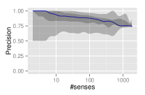
(a) $\mathcal{A}_{2}$

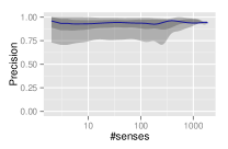
(b) $\mathcal{B}$

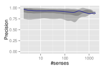
(c) $\mathcal{C}$

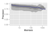
(d) $\mathcal{D}$

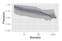
(e) $\mathcal{E}$

Figure 2: Per-mention precision for all datasets: the blue line is a smoothed median of precision values and the two ribbons correspond to the two smoothed quantile intervals $(5\%,95\%)$ and $(25\%,75\%)$

10 Conclusions

This paper proposes a new per-mention learning (PML) disambiguation system, in which the feature engineering and model training is done per unique mention. The most significant advantage of this approach lies in the specialized learning that improves the precision. The method is also highly parallelizable and scalable, and can be further tuned for higher precision with per-mention or per-candidate pruning. Furthermore, this per-mention disambiguation approach can be easily calibrated or tuned for specific mentions with new datasets, without affecting the results of other mentions. In an extensive comparisons with $10$ other disambiguation systems over $11$ different datasets, we have shown that our PML system is very competitive with the state-of-the-art, and, for the specific case ofdisambiguating news, consistently outperforms these other systems.

There are several potential key tasks that we consider for future work. Firstly, we wish to combine PML with graph-based approaches for further improvement. One method is to impose coherence between chosen senses in the same document or sentence, by using a fast graph-based approach on the top-$k$ results of our proposed disambiguation. Secondly, the computational bottle neck of our system for new annotations lies in the set matching operation between annotation and sense context, which can be improved with an optimized algorithm.

References

- [1] D. Carmel, M.-W. Chang, E. Gabrilovich, B.-J. P. Hsu, and K. Wang. ERD’14: Entity recognition and disambiguation challenge. SIGIR Forum, 48(2):63–77, Dec. 2014.
- [2] S. Cucerzan. Large-scale named entity disambiguation based on wikipedia data. In Proceedings of EMNLP-CoNLL 2007, pages 708–716, June 2007.
- [3] S. Cucerzan. Name entities made obvious: the participation in the ERD 2014 evaluation. In Proceedings of the First International Workshop on Entity Recognition & Disambiguation, ERD, pages 95–100, New York, NY, USA, 2014. ACM.
- [4] J. Daiber, M. Jakob, C. Hokamp, and P. N. Mendes. Improving efficiency and accuracy in multilingual entity extraction. In Proceedings of the 9th International Conference on Semantic Systems, I-SEMANTICS, 2013.
- [5] P. Ferragina and U. Scaiella. Fast and accurate annotation of short texts with Wikipedia pages. ArXiv e-prints, June 2010.
- [6] P. Ferragina and U. Scaiella. TAGME: On-the-fly annotation of short text fragments (by Wikipedia entities). In Proceedings of the 19th ACM International Conference on Information and Knowledge Management, CIKM, pages 1625–1628, 2010.
- [7] D. A. Ferrucci. Introduction to ”This is Watson”. IBM Journal of Research and Development, 56(3):235–249, May 2012.
- [8] O. Ganea, M. Ganea, A. Lucchi, C. Eickhoff, and T. Hofmann. Probabilistic bag-of-hyperlinks model for entity linking. In Proceedings of the 25th International Conference on World Wide Web, WWW 2016, Montreal, Canada, April 11 - 15, 2016, pages 927–938, 2016.
- [9] Z. Guo and D. Barbosa. Robust entity linking via random walks. In Proceedings of the 23rd ACM International Conference on Conference on Information and Knowledge Management, CIKM 2014, Shanghai, China, November 3-7, 2014, pages 499–508, 2014.
- [10] X. Han and L. Sun. A generative entity-mention model for linking entities with knowledge base. In Proceedings of the 49th Annual Meeting of the Association for Computational Linguistics: Human Language Technologies, HLT, pages 945–954, 2011.
- [11] X. Han, L. Sun, and J. Zhao. Collective entity linking in web text: A graph-based method. In Proceedings of the 34th International ACM SIGIR Conference on Research and Development in Information Retrieval, SIGIR, pages 765–774, 2011.
- [12] J. Hoffart. Discovering and disambiguating named entities in text. In Proceedings of the 2013 SIGMOD/PODS Ph.D. Symposium, SIGMOD PhD Symposium, pages 43–48, 2013.
- [13] I. Hulpus, N. Prangnawarat, and C. Hayes. Path-based semantic relatedness on linked data and its use to word and entity disambiguation. In Proceedings of the 14th International Semantic Web Conference ISWC, pages 442–457, 2015.
- [14] S. Kulkarni, A. Singh, G. Ramakrishnan, and S. Chakrabarti. Collective annotation of Wikipedia entities in web text. In Proceedings of the 15th ACM SIGKDD International Conference on Knowledge Discovery and Data Mining, KDD, pages 457–466, 2009.
- [15] P. McNamee. HLTCOE efforts in entity linking at TAC KBP 2010. In Proceedings of the TAC 2010 Workshop, 2010.
- [16] E. Meij, W. Weerkamp, and M. de Rijke. Adding semantics to microblog posts. In Proceedings of the Fifth International Conference on Web Search and Web Data Mining, WSDM, pages 563–572, 2012.
- [17] D. Milne and I. H. Witten. Learning to link with Wikipedia. In Proceedings of the 17th ACM Conference on Information and Knowledge Management, CIKM, pages 509–518, 2008.
- [18] A. Moro, A. Raganato, and R. Navigli. Entity linking meets word sense disambiguation: a unified approach. Transactions of the Association for Computational Linguistics, 2:231–244, 2014.
- [19] A. Olieman, H. Azarbonyad, M. Dehghani, J. Kamps, and M. Marx. Entity linking by focusing DBpedia candidate entities. In Proceedings of the First International Workshop on Entity Recognition & Disambiguation, ERD, pages 13–24, 2014.
- [20] F. Piccinno and P. Ferragina. From TAGME to WAT: A new entity annotator. In Proceedings of the First International Workshop on Entity Recognition & Disambiguation, ERD, pages 55–62, 2014.
- [21] M. A. Qureshi, C. O’Riordan, and G. Pasi. Exploiting wikipedia for entity name disambiguation in tweets. In Natural Language Processing and Information Systems - 19th International Conference on Applications of Natural Language to Information Systems, NLDB, pages 184–195, 2014.
- [22] F. Suchanek and G. Weikum. Knowledge harvesting in the big-data era. In Proceedings of the 2013 ACM SIGMOD International Conference on Management of Data, SIGMOD, pages 933–938, New York, NY, USA, 2013. ACM.
- [23] R. Usbeck, A. N. Ngomo, M. Röder, D. Gerber, S. A. Coelho, S. Auer, and A. Both. AGDISTIS - agnostic disambiguation of named entities using linked open data. In Proceedings of the 21st European Conference on Artificial Intelligence ECAI, pages 1113–1114, 2014.
- [24] R. Usbeck, M. Röder, A.-C. Ngonga Ngomo, C. Baron, A. Both, M. Brümmer, D. Ceccarelli, M. Cornolti, D. Cherix, B. Eickmann, P. Ferragina, C. Lemke, A. Moro, R. Navigli, F. Piccinno, G. Rizzo, H. Sack, R. Speck, R. Troncy, J. Waitelonis, and L. Wesemann. GERBIL: general entity annotator benchmarking framework. In Proceedings of the 24th International Conference on World Wide Web, WWW, pages 1133–1143, 2015.