Vector chirality for effective total momentum $J_{\textrm{eff}}$ in a nonfrustrated Mott insulator: Effects of strong spin-orbit coupling and broken inversion symmetry

Abstract

I propose the emergence of the spin-orbital-coupled vector chirality in a non-frustrated Mott insulator with the strong spin-orbit coupling due to $ab$-plane’s inversion-symmetry (IS) breaking. I derive the superexchange interactions for a $t_{2g}$-orbital Hubbard model on a square lattice with the strong spin-orbit coupling and the IS-breaking-induced hopping integrals, and explain the microscopic origins of the Dzyaloshinsky-Moriya (DM) -type and the Kitaev-type interactions. Then, by adopting the mean-field approximation to a minimal model including only the Heisenberg-type and the DM-type nearest-neighbor interactions, I show that the IS breaking causes the spin-orbital-coupled chirality as a result of stabilizing the screw state. I also highlight the limit of the hard-pseudospin approximation in discussing the stability of the screw states in the presence of both the DM-type and the Kitaev-type interactions, and discuss its meaning. I finally discuss the effects of tetragonal crystal field and $J_{\textrm{eff}}=\frac{3}{2}$ states, and the application to the iridates near the $[001]$ surface of Sr₂IrO₄ and the interface between Sr₂IrO₄ and Sr₃Ir₂O₇.

I Introduction

The spin chirality is a key concept in condensed-matter physics. That is categorized as either vector-type one, $\bm{S}_{\bm{i}}\times\bm{S}_{\bm{j}}$, or scalar-type one, $\bm{S}_{\bm{i}}\cdot(\bm{S}_{\bm{j}}\times\bm{S}_{\bm{k}})$. One of the former’s drastic effects is to generate the electric polarization in multiferroic materials such as TbMnO₃ multiferro-exp ; multiferro-Nagaosa ; multiferro-theory ; multiferro-1stPrinc ; for the latter, its drastic effect is to cause the anomalous-Hall effect in a frustrated system such as Pr₂Ir₂O₇ chirality-AHE-exp ; chirality-AHE-Udagawa . In addition to those, the spin chirality is related to skyrmion physics skrymion and heavy-fermion physics chirality-HF .

There are two mechanisms for realizing the spin chirality. One arises from the Dzyaloshinsky-Moriya(DM)-type antisymmetric exchange interaction DM1 ; DM2 such as $\textstyle\sum_{\bm{i},\bm{j}}\bm{D}_{\bm{i},\bm{j}}\cdot(\bm{S}_{\bm{i}}\times\bm{S}_{\bm{j}})$ with $\bm{D}_{\bm{i},\bm{j}}=-\bm{D}_{\bm{j},\bm{i}}$. In the system in which inversion symmetry (IS) is broken due to lattice distortion, such DM-type interaction appears as a result of the combination effects of the onsite spin-orbit coupling (SOC), the kinetic exchange, and the IS breaking DM2 ; the DM-type interaction induces the spin vector chirality. This mechanism works in $\alpha$-Fe₂O₃, for example DM2 . The other arises from the competition spiral between the Heisenberg-type symmetric exchange interactions such as $\textstyle\sum_{\bm{i},\bm{j}}J_{\bm{i},\bm{j}}\bm{S}_{\bm{i}}\cdot\bm{S}_{\bm{j}}$ with $J_{\bm{i},\bm{j}}=J_{\bm{j},\bm{i}}$; this does not need lattice origin’s IS breaking. Its example is MnO₂ spiral : in a body-centered unit cell the Heisenberg-type interactions between the nearest-neighbor (NN) sites along the $c$ axis compete with others between the body center and each vertex; this competition results in stabilizing a screw state, where the spin vector chirality becomes finite.

Although the understanding of the spin chirality has been developed, the chirality of another degree of freedom is unsatisfactorily understood. For example, we little understand the chirality of the orbital, although its possibility may be suggested by the close similarities between the spin and the orbital about orders and fluctuations Tokura-Nagaosa . Since the orbital degree of freedom of an electron describes the anisotropy of its spatial distribution, the understanding of the chirality of the orbital may open a new possibility of utilizing the chirality of the anisotropic spatial distribution of electrons/holes. Although there are several studies related to the chirality of the orbital, these focused on the frustrated iridates hyperkagomeIr-Balents ; hyperkagomeIr-Shindou ; hyperkagomeIr-Mizoguchi ; honeycombIr-exp ; honeycombIr-zigzag ; honeycombIr-YBKim , the Ir oxides with the geometric frustration of the symmetric exchange interactions. Since the frustration tends to develop the strong fluctuations, it is difficult to realize the chirality of the orbital as a result of the order; if it is realized, it may be easily broken by a small perturbation because such perturbation is sufficient to stabilize another competed state. Thus, the nonfrustrated system may be better for studies towards realizing the chirality related to the orbital and utilizing and controlling it. However, it has been unclear whether the chirality related to the orbital is realized in the nonfrustrated system with the strong SOC because of lattice origin’s IS breaking, although the realization may be suggested by the analogy with the case of the spin chirality in a nonfrustrated system with the weak SOC. Thus, we should clarify the possibility of the chirality related to the orbital in a non-frustrated system with the strong SOC in the presence of the IS breaking.

Here I propose that a nonfrustrated Mott insulator with the strong SOC gains the spin-orbital-coupled vector chirality by introducing the IS breaking on an $ab$ plane due to the DM-type interactions for the spin-orbital-coupled degree of freedom Ir214-Jeff-PRL ; Ir214-Jeff-Science , $\bm{J}_{\bm{i}}=\bm{S}_{\bm{i}}-\bm{L}_{\bm{i}}$ for $J_{\textrm{eff}}=1/2$. Focusing on the essential effects of the IS breaking on the low-energy physics of a quasi-two-dimensional insulating iridate, I derive the superexchange interactions for a $t_{2g}$-orbital Hubbard model with the strong SOC on a square lattice without $ab$-plane’s IS, and explain why the IS breaking leads to the DM-type and the Kitaev-type Kitaev interactions. Then, by using the mean-field approximation, I show the emergence of the spin-orbital-coupled vector chirality in a minimal model with only the Heisenberg-type and the DM-type NN interactions as a result of stabilizing the screw state. Although even in the presence of the anisotropic terms such as the Kitaev-type interactions the screw state gives the lowest energy, the hard-pseudospin constraints are violated. This suggests the limit of the hard-pseudospin approximation in discussing the stability of the screw states in the presence of both the DM-type and the Kitaev-type interactions. I finally discuss the validity of the treatment of effects of tetragonal crystal field and the $J_{\textrm{eff}}=\frac{3}{2}$ states, and a possibility of the spin-orbital-coupled vector chirality near the $[001]$ surface of Sr₂IrO₄ and the interface between Sr₂IrO₄ and Sr₃Ir₂O₇. Hereafter we set $\hbar=1$ and choose the lattice constants as unity.

II Method

II.1 Model

We use a $t_{2g}$-orbital Hubbard model with the onsite SOC on a square lattice as an effective model of a quasi-two-dimensional iridate, and treat the effects of the IS breaking on an $ab$ plane as the NN hoppings Yanase-ISB ; Mizoguchi-SHE between the $d_{xy}$ and $d_{yz}$ orbitals along the $x$ direction, and between the $d_{xy}$ and $d_{xz}$ orbitals along the $y$ direction. (Such treatment is appropriate for a $t_{2g}$-orbital system, and its applicability is wider than a single-orbital Rashba model Mizoguchi-SHE .) Namely, the Hamiltonian becomes

$$\hat{H}=\hat{H}_{\textrm{even}}+\hat{H}_{LS}+\hat{H}_{\textrm{int}}+\hat{H}_{\textrm{odd}},$$ (1)

where $\hat{H}_{\textrm{even}}$ represents the kinetic energy,

$$\hat{H}_{\textrm{even}}=\sum\limits_{\bm{i},\bm{j}}\sum\limits_{a,b}\sum\limits_{s}t_{ab;\bm{i}\bm{j}}^{(\textrm{even})}\hat{c}_{\bm{i}as}^{\dagger}\hat{c}_{\bm{j}bs},$$ (2)

with site indices, $\bm{i}$ and $\bm{j}$, for $N$ sites, orbital indices, $a,b=d_{xz},d_{yz},d_{xy}$, a spin index, $s=\uparrow,\downarrow$, and even-mirror hopping integrals, the hopping integrals even about $ab$-plane’s mirror symmetry, given in Fig. 1; $\hat{H}_{LS}$ the onsite SOC,

$$\hat{H}_{LS}=(-\lambda_{LS})\sum\limits_{\bm{i}}\sum\limits_{a,b}\sum\limits_{s,s^{\prime}}(\bm{l}_{\bm{i}}\cdot\bm{s}_{\bm{i}})_{asbs^{\prime}}\hat{c}_{\bm{i}as}^{\dagger}\hat{c}_{\bm{i}bs^{\prime}},$$ (3)

with the standard matrix elements $(\bm{l}_{\bm{i}}\cdot\bm{s}_{\bm{i}})_{asbs^{\prime}}$ (e.g., see Ref. Mizoguchi-SHE, ); $\hat{H}_{\textrm{int}}$ the multiorbital Hubbard interactions,

$$\hat{H}_{\textrm{int}}=\sum\limits_{\bm{i}}\sum\limits_{a,b}\hat{c}_{\bm{i}a\uparrow}^{\dagger}\hat{c}_{\bm{i}a\downarrow}^{\dagger}[U\delta_{b,a}+J^{\prime}(1-\delta_{b,a})]\hat{c}_{\bm{i}b\downarrow}\hat{c}_{\bm{i}b\uparrow}$$

$$+ \sum\limits_{\bm{i}}\sum\limits_{a,b(<a)}\sum\limits_{s,s^{\prime}}\hat{c}_{\bm{i}as}^{\dagger}\hat{c}_{\bm{i}bs^{\prime}}^{\dagger}[U^{\prime}\hat{c}_{\bm{i}bs^{\prime}}\hat{c}_{\bm{i}as}-J_{\textrm{H}}\hat{c}_{\bm{i}bs}\hat{c}_{\bm{i}as^{\prime}}];$$ (4)

$\hat{H}_{\textrm{odd}}$ the Hamiltonian induced by the IS breaking Yanase-ISB ; Mizoguchi-SHE ,

$$\hat{H}_{\textrm{odd}}=\sum\limits_{\bm{i},\bm{j}}\sum\limits_{a,b}\sum\limits_{s}t_{ab;\bm{i}\bm{j}}^{(\textrm{odd})}\hat{c}_{\bm{i}as}^{\dagger}\hat{c}_{\bm{j}bs},$$ (5)

with odd-mirror hopping integral, the hopping integral odd about $ab$-plane’s mirror symmetry, given in Fig. 1.

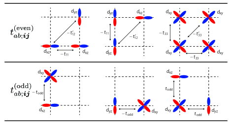
Figure 1: Schematic pictures of finite $t_{ab;\bm{i}\bm{j}}^{(\textrm{even})}$ and $t_{ab;\bm{i}\bm{j}}^{(\textrm{odd})}$ on a square lattice. The NN hoppings arise from the indirect ones through the $2p$ orbitals of an O ion, and the next-NN hoppings arise from the direct ones.

In our Hamiltonian, we neglect the tetragonal crystal field; the validity will be discussed in Sec. IV. In the analyses, we consider a hole per site because the iridates have the $(t_{2g})^{5}$-electron configuration Ir214-Jeff-PRL , equivalent to the $(t_{2g})^{1}$-hole configuration.

Before the derivation of the low-energy superexchange interactions, I briefly validate the appearance of the odd-mirror hopping integral in the absence of $ab$-plane’s IS. For that purpose, it would be better to begin with the symmetrical properties of the hopping integrals permissible in a square lattice with $ab$-plane’s IS. In the presence of $ab$-plane’s IS, the permissible hopping integrals for the $t_{2g}$ orbitals should be even about $z$. Furthermore, the permissible hopping integrals along the $x$ and $y$ directions should be even about $y$ and even about $x$, respectively. Actually, those properties hold for all the hopping integrals of $\hat{H}_{\textrm{even}}$ because the wave functions of the $d_{xz}$, $d_{yz}$, and $d_{xy}$ orbitals behave like $xz$, $yz$, and $xy$, respectively, in symmetrical operations; e.g., the NN hopping integral of the $d_{xz}$ orbital along the $x$ direction, behaving like $xz\cdot xz=x^{2}y^{0}z^{2}$, is even about $y$ and $z$. Then, in the absence of $ab$-plane’s IS, the hopping integrals odd about $z$, the odd-mirror hopping integrals, become permissible. As a result, the NN hopping integral between the $d_{yz}$ and the $d_{xy}$ orbitals along the $x$ direction is possible because that behaves like $yz\cdot xy=x^{1}y^{2}z^{1}$, which is odd about $z$ and even about $y$. In addition, the NN hopping integral between the $d_{xz}$ and the $d_{xy}$ orbitals along the $y$ direction is possible. However, the NN hopping integral either between the $d_{xz}$ and the $d_{xy}$ orbitals along the $x$ direction or between the $d_{yz}$ and the $d_{xy}$ orbitals along $y$ direction is prohibited even in the absence of $ab$-plane’s IS. This is because the former is odd about $y$ and the latter is odd about $x$, and because $ab$-plane’s IS breaking does not affect the symmetrical properties about $x$ and $y$. The above explanations are the reason why $ab$-plane’s IS breaking induces the odd-mirror hopping integrals. Those hopping integrals are not only odd mirror but also odd parity because the IS breaking considered is the same at each site, i.e. its effects are uniform.

II.2 Low-energy superexchange interactions

To understand the low-energy physics of $\hat{H}$, we derive the superexchange interactions Superex-Anderson ; Superex-KK in a strong-correlation limit. Here I will show the result for $J^{\prime}=J_{\textrm{H}}=0$ and $U^{\prime}=U$ in $U,U^{\prime}\gg\lambda_{LS}\gg|t_{ab;\bm{i}\bm{j}}^{(\textrm{even})}|,|t_{ab;\bm{i}\bm{j}}^{(\textrm{odd})}|$ honeycombIr-zigzag ; hyperkagomeIr-Mizoguchi in order to focus on the essential effects of the IS breaking as simply as possible. Its effects on the superexchange interactions remain qualitatively the same as the case for $J^{\prime}>0$, $J_{\textrm{H}}>0$, and $U^{\prime}<U$ (see Appendix A). Including the effects of $\hat{H}_{LS}$ as the formation of the $J=\frac{1}{2}$ states honeycombIr-zigzag , rewriting $\hat{H}_{\textrm{int}}$ in terms of the irreducible representations of the intermediate states Superex-titanates , treating $\hat{H}_{\textrm{even}}+\hat{H}_{\textrm{odd}}$ in the second-order perturbation, and setting $J^{\prime}=J_{\textrm{H}}=0$ and $U^{\prime}=U$, we obtain an effective Hamiltonian (for more details see Appendix A):

$$\hat{H}_{\textrm{eff}}=J_{1}\sum\limits_{\langle\bm{i},\bm{j}\rangle}\hat{\bm{J}}_{\bm{i}}\cdot\hat{\bm{J}}_{\bm{j}}+J_{2}\sum\limits_{\langle\langle\bm{i},\bm{j}\rangle\rangle}\hat{\bm{J}}_{\bm{i}}\cdot\hat{\bm{J}}_{\bm{j}}+D\sum\limits_{\langle\bm{i},\bm{j}\rangle_{x}}(\hat{\bm{J}}_{\bm{i}}\times\hat{\bm{J}}_{\bm{j}})^{y}$$

$$-D\sum\limits_{\langle\bm{i},\bm{j}\rangle_{y}}(\hat{\bm{J}}_{\bm{i}}\times\hat{\bm{J}}_{\bm{j}})^{x}+K\sum\limits_{\langle\bm{i},\bm{j}\rangle_{x}}\hat{J}_{\bm{i}}^{y}\hat{J}_{\bm{j}}^{y}+K\sum\limits_{\langle\bm{i},\bm{j}\rangle_{y}}\hat{J}_{\bm{i}}^{x}\hat{J}_{\bm{j}}^{x},$$ (6)

with

$$J_{1}=\frac{4}{9}\frac{(t_{11}+t_{33})^{2}}{U}-\frac{16}{9}\frac{(t_{\textrm{odd}})^{2}}{U}=J_{0}-J_{\textrm{odd}},$$ (7)

$$J_{2}=\frac{4}{9}\frac{(t_{33}^{\prime})^{2}}{U},$$ (8)

$$D=\frac{16}{9}\frac{t_{\textrm{odd}}(t_{11}+t_{33})}{U},$$ (9)

$$K=2J_{\textrm{odd}},$$ (10)

$\textstyle\sum_{\langle\bm{i},\bm{j}\rangle}=\textstyle\sum_{\langle\bm{i},\bm{j}\rangle_{x}}+\textstyle\sum_{\langle\bm{i},\bm{j}\rangle_{y}}$, the sum of the summations taken over the NN sites along the $x$ and $y$ directions, and $\textstyle\sum_{\langle\langle\bm{i},\bm{j}\rangle\rangle}$, the summation taken over the next-NN sites. Here we have neglected the products of the hole-density operators such as $\textstyle\sum_{\langle\bm{i},\bm{j}\rangle}\hat{n}_{\bm{i}}\hat{n}_{\bm{j}}$ because such terms become constants in the mean-field approximation. Note that the finite terms of the DM-type interaction in Eq. (6) differ from the rotation-induced DM-type interaction Ir214-weakFM-theory . In Sec. IV, we will discuss the effect of the $J_{\textrm{eff}}=\frac{3}{2}$ states on the superexchange interactions.

The derived effective Hamiltonian Eq. (6) shows three effects of the IS breaking. One is to cause the DM-type interactions, $D\textstyle\sum_{\langle\bm{i},\bm{j}\rangle_{x}}(\hat{\bm{J}}_{\bm{i}}\times\hat{\bm{J}}_{\bm{j}})^{y}$ and $-D\textstyle\sum_{\langle\bm{i},\bm{j}\rangle_{y}}(\hat{\bm{J}}_{\bm{i}}\times\hat{\bm{J}}_{\bm{j}})^{x}$. Those interactions arise from the multiorbital superexchange interactions due to the combination of the even-mirror and the odd-mirror hopping integrals. Such combination is vital to obtain the DM-type antisymmetric interactions. This is because their operator parts behave like the functions odd about some coordinates in the symmetrical operations. For example, $(\hat{\bm{J}}_{\bm{i}}\times\hat{\bm{J}}_{\bm{j}})^{x}=\hat{J}^{y}_{\bm{i}}\hat{J}^{z}_{\bm{j}}-\hat{J}^{z}_{\bm{i}}\hat{J}^{y}_{\bm{j}}$ behaves like the function which is odd about $y$ and $z$ (and even about $x$); such function can be obtained by the multiorbital superexchange interactions using the even-mirror hopping integral and the odd-mirror hopping integral between the $d_{xz}$ and the $d_{xy}$ orbitals, which behaves like $xz\cdot xy=x^{2}y^{1}z^{1}$. Thus, the DM-type interactions originate from the mirror-mixing multiorbital effect. Another effect is to cause the ferromagnetic Heisenberg-type interaction, $-J_{\textrm{odd}}\textstyle\sum_{\langle\bm{i},\bm{j}\rangle}\hat{\bm{J}}_{\bm{i}}\cdot\hat{\bm{J}}_{\bm{j}}$. This interaction between the $z$ components arises from a larger gain of the energy reduction due to the kinetic exchange between the same-$J^{z}$ states than between the opposite-$J^{z}$ states. This is because the number of processes in the former case is larger due to the opposite spin indices between the $d_{xy}$ orbital and the $d_{xz}$ or $d_{yz}$ orbital in the $J^{z}=\pm\frac{1}{2}$ states Rigand-text . Then, by including the pseudospin-flipping processes, we can obtain the ferromagnetic Heisenberg-type interaction because these processes give the $\hat{J}_{\bm{i}}^{+}\hat{J}_{\bm{j}}^{+}$ or $\hat{J}_{\bm{i}}^{-}\hat{J}_{\bm{j}}^{-}$ terms. The other effect is to cause the antiferromagentic Kitaev-type interactions, $K\textstyle\sum_{\langle\bm{i},\bm{j}\rangle_{x}}\hat{J}_{\bm{i}}^{y}\hat{J}_{\bm{j}}^{y}$ and $K\textstyle\sum_{\langle\bm{i},\bm{j}\rangle_{y}}\hat{J}_{\bm{i}}^{x}\hat{J}_{\bm{j}}^{x}$. This is because the above $J_{\bm{i}}^{+}J_{\bm{j}}^{+}$ or $\hat{J}_{\bm{i}}^{-}\hat{J}_{\bm{j}}^{-}$ terms give the extra $\hat{J}_{\bm{i}}^{x}\hat{J}_{\bm{j}}^{x}$ or $J_{\bm{i}}^{y}J_{\bm{j}}^{y}$ terms, and because the orbitals hybridized by $\hat{H}_{\textrm{odd}}$ along the $x$ and $y$ direction have the finite off-diagonal matrix elements only of $\hat{L}_{\bm{i}}^{y}$ or $\hat{L}_{\bm{i}}^{x}$, respectively. Namely, the superexchange interactions between $\hat{L}_{\bm{i}}^{y}$ and $\hat{L}_{\bm{j}}^{y}$ along the $x$ direction and between $\hat{L}_{\bm{i}}^{x}$ and $\hat{L}_{\bm{j}}^{x}$ along the $y$ direction become antiferromagnetic in order to gain the energy reduction of the kinetic exchange due to the spin-independent interorbital hoppings of $\hat{H}_{\textrm{odd}}$, resulting in the antiferromagnetic Kitaev-type interactions.

II.3 Mean-field approximation

For further understanding of the effects of the IS breaking, we analyze the ground state of Eq. (6) in the mean-field approximation. Since the energy in this approximation is quadratic about $\langle\hat{J}_{\bm{q}}^{\alpha}\rangle=\frac{1}{\sqrt{N}}\textstyle\sum_{\bm{j}}e^{-i\bm{q}\cdot\bm{j}}\langle\hat{J}_{\bm{j}}^{\alpha}\rangle$, i.e.

$$\langle\hat{H}_{\textrm{eff}}\rangle=\sum\limits_{\bm{q}}\sum\limits_{\alpha,\beta=x,y,z}J_{\alpha\beta}(\bm{q})\langle\hat{J}_{\bm{q}}^{\alpha}\rangle^{\ast}\langle\hat{J}_{\bm{q}}^{\beta}\rangle,$$ (11)

we can determine the ground state by finding $\bm{q}$ of the lowest eigenvalue and the eigenvector of Eq. (11) with the periodic boundary condition and the constraints of the hard-pseudospin approximation,

$$\frac{1}{4}= \frac{1}{N}\sum\limits_{\alpha}\sum\limits_{\bm{q},\bm{q}^{\prime}}e^{i(\bm{q}^{\prime}-\bm{q})\cdot\bm{j}}\langle\hat{J}_{\bm{q}}^{\alpha}\rangle^{\ast}\langle\hat{J}_{\bm{q}^{\prime}}^{\alpha}\rangle,$$ (12)

in which $\langle\hat{J}_{\bm{i}}^{\alpha}\rangle$ for all $N$ sites are treated as the hard pseudospins for $J_{\textrm{eff}}=\frac{1}{2}$. In Eq. (11), $J_{\alpha\beta}(\bm{q})$ are given by

$$J_{xx}(\bm{q})= (J_{0}-J_{\textrm{odd}})\cos q_{x}+(J_{0}+J_{\textrm{odd}})\cos q_{y}$$

$$+4J_{2}\cos q_{x}\cos q_{y},$$ (13)

$$J_{yy}(\bm{q})= (J_{0}+J_{\textrm{odd}})\cos q_{x}+(J_{0}-J_{\textrm{odd}})\cos q_{y}$$

$$+4J_{2}\cos q_{x}\cos q_{y},$$ (14)

$$J_{zz}(\bm{q})= (J_{0}-J_{\textrm{odd}})\cos q_{x}+(J_{0}-J_{\textrm{odd}})\cos q_{y}$$

$$+4J_{2}\cos q_{x}\cos q_{y},$$ (15)

$$J_{zx}(\bm{q})= \ iD\sin q_{x},$$ (16)

$$J_{xz}(\bm{q})= -iD\sin q_{x},$$ (17)

$$J_{zy}(\bm{q})= \ iD\sin q_{y},$$ (18)

$$J_{yz}(\bm{q})= -iD\sin q_{y}.$$ (19)

The derivation of Eq. (11) from Eq. (6) is described in Appendix B.

III Results

Before the analyses with the IS breaking, we briefly explain the ground state without the IS breaking. Without it, the ground state is determined by the $J_{0}$ term and the $J_{2}$ term of Eq. (6). Namely, the ground state is a $(\pi,\pi)$-antiferromagnetic state for $J_{0}>4J_{2}$, and a $(\pi,0)$- or $(0,\pi)$-antiferromagnetic state for $J_{0}<4J_{2}$. The former is realized in a realistic case because $J_{0}>4J_{2}$ is satisfied due to $|t_{11}|\sim|t_{33}|$ and $|t_{33}^{\prime}|<|t_{33}|$ Ir214-Watanabe .

III.1 Stability of the screw states

To understand how the IS breaking affects the $(\pi,\pi)$-antiferromagnetic state, realized without the IS breaking, let us consider a minimal model with only the $J_{0}$ term and the $D$ terms of Eq. (6). This minimal model is reasonable to analyze the essential effects of the IS breaking because $D$ is larger than $K$ for $2|t_{\textrm{odd}}|<|t_{11}+t_{33}|$, corresponding to the case with the small effects of the IS breaking. (Such small-effect case is considered because the small effects are realized as long as the IS is broken.) For this minimal model, the lowest eigenvalue of Eq. (11) for each $\bm{q}$ is determined by

$$\lambda(\bm{q})=J_{0}(\cos q_{x}+\cos q_{y})-|D|\sqrt{(\sin q_{x})^{2}+(\sin q_{y})^{2}},$$ (20)

and it has three kinds of local minimum: (i) the $(\pi,\pi)$-antiferromagnetic state,

$$\lambda(\bm{Q}_{\textrm{AF}})=-2J_{0}$$ (21)

with $\bm{Q}_{\textrm{AF}}=(\pi,\pi)$; (ii) the one-directional-screw state,

$$\lambda(\bm{Q}_{1})=-J_{0}-\sqrt{J_{0}^{2}+D^{2}}$$ (22)

with $\bm{Q}_{1}=(\pm Q_{1},\pi)$ or $\bm{Q}_{1}=(\pi,\pm Q_{1})$ for $Q_{1}=\pi-\cos^{-1}(J_{0}/\sqrt{J_{0}^{2}+D^{2}})$; and (iii) the two-directional-screw state,

$$\lambda(\bm{Q}_{2})=-\sqrt{2}\sqrt{2J_{0}^{2}+D^{2}}$$ (23)

with $\bm{Q}_{2}=(\pm Q_{2},\pm Q_{2})$ or $\bm{Q}_{2}=(\pm Q_{2},\mp Q_{2})$ for $Q_{2}=\pi-\cos^{-1}(\sqrt{2}J_{0}/\sqrt{2J_{0}^{2}+D^{2}})$.

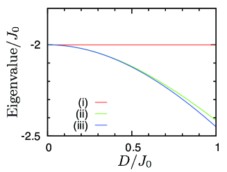
Figure 2: $(D/J_{0})$ dependences of the eigenvalues divided by $J_{0}$ for states (i), (ii), and (iii) in the mean-field approximation for the minimal model.

In contrast to the $(\pi,\pi)$-antiferromagnetic state, those screw states show two unusual features. One is the spatial-dependent mixing between or among the components of $\langle\hat{J}_{\bm{i}}^{\alpha}\rangle$: for example, in the one-directional-screw state for $\bm{Q}_{1}=(\pm Q_{1},\pi)$,

$$\langle\hat{\bm{J}}_{\bm{i}}\rangle=\frac{1}{2}\left(\begin{array}[]{@{\,}c@{\,}}(-1)^{i_{y}+1}\textrm{sgn}(D)\sin Q_{1}i_{x}\\ 0\\ (-1)^{i_{y}}\cos Q_{1}i_{x}\end{array}\right);$$ (27)

and in the two-directional-screw state for $\bm{Q}_{2}=(\pm Q_{2},\pm Q_{2})$,

$$\langle\hat{\bm{J}}_{\bm{i}}\rangle=\frac{1}{2}\left(\begin{array}[]{@{\,}c@{\,}}-\frac{1}{\sqrt{2}}\textrm{sgn}(D)\sin\bm{Q}_{2}\cdot\bm{i}\\ -\frac{1}{\sqrt{2}}\textrm{sgn}(D)\sin\bm{Q}_{2}\cdot\bm{i}\\ \cos\bm{Q}_{2}\cdot\bm{i}\end{array}\right).$$ (31)

Thus, those screw states have the spatial variation of not only the spin distribution but also the orbital distribution because the spin and the orbital are highly entangled in the $J_{\textrm{eff}}=\frac{1}{2}$ states Rigand-text [see Eqs. (35) and (36)]. The other is the finite vector chirality: for example, in the one-directional-screw state for $\bm{Q}_{1}=(\pm Q_{1},\pi)$, the finite term is

$$\langle(\hat{\bm{J}}_{\bm{i}}\times\hat{\bm{J}}_{\bm{j}})^{y}\rangle=\frac{1}{4}(-1)^{i_{y}+j_{y}}\textrm{sgn}(D)\sin Q_{1}(j_{x}-i_{x});$$ (32)

and in the two-directional-screw state for $\bm{Q}_{2}=(\pm Q_{2},\pm Q_{2})$, the finite terms are

$$\langle(\hat{\bm{J}}_{\bm{i}}\times\hat{\bm{J}}_{\bm{j}})^{x}\rangle=\frac{1}{4\sqrt{2}}\textrm{sgn}(D)\sin\bm{Q}_{2}\cdot(\bm{j}-\bm{i})$$ (33)

and

$$\langle(\hat{\bm{J}}_{\bm{i}}\times\hat{\bm{J}}_{\bm{j}})^{y}\rangle=-\frac{1}{4\sqrt{2}}\textrm{sgn}(D)\sin\bm{Q}_{2}\cdot(\bm{j}-\bm{i}).$$ (34)

Thus, those screw states have the spin-orbital-coupled vector chirality.

From the $(D/J_{0})$ dependences of the eigenvalues of states (i), (ii), and (iii), shown in Fig. 2, we find that the screw states are more stable than the $(\pi,\pi)$-antiferromagnetic state, and that the most stable state in the minimal model is the two-directional-screw state. The stabilities of those screw states can be understood that the $J_{0}$ term becomes minimum for $\bm{q}=(\pi,\pi)$, and the $D$ terms become minimum for $\bm{q}=(\frac{\pi}{2},\frac{\pi}{2})$.

III.2 Limit of the hard-pseudospin approximation

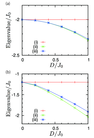
Figure 3: $(D/J_{0})$ dependences of the eigenvalues divided by $J_{0}$ for states (i), (ii), and (iii) in the mean-field approximation with $N=100\times 100$ meshes for the model with the $J_{0}$ and the $D$ terms, $J_{\textrm{odd}}=\frac{1}{4}J_{0}(\frac{D}{J_{0}})^{2}$, and $J_{2}=$ (a) $0$ or (b) $0.2J_{0}$.

Even in the presence of the $J_{2}$ term and the $J_{\textrm{odd}}$ terms, the eigenvalues of the screw states are lower than the eigenvalue for $\bm{q}=(\pi,\pi)$, as shown in Figs. 3(a) and 3(b). In particular, the one-directional-screw state for $\bm{Q}_{1}^{\prime}=(\pm Q_{1}^{\prime},\pi)$ or $\bm{q}=(\pi,\pm Q_{1}^{\prime})$ gives the lowest eigenvalue (see those figures). This is because the $J_{\textrm{odd}}$ terms and the $J_{2}$ term destabilize the states for $\bm{q}=(Q,\pm Q)$. Namely, the lowest eigenvalue of the one-directional-screw state arises from the combination of the stabilization of the screw states due to the $D$ terms and the destabilization of the two-directional-screw state (compared with the one-directional-screw state) due to the $J_{\textrm{odd}}$ terms and the $J_{2}$ term.

In contrast to the case of the minimal model, the screw states in the presence of the $J_{\textrm{odd}}$ terms do not satisfy the hard-pseudospin constraints of $\langle\hat{\bm{J}}_{\bm{j}}\rangle$. This is because under the constraints, the possible one-directional-screw state is restricted to $\langle\hat{\bm{J}}_{\bm{Q}}\rangle={}^{t}(\pm ib,0,b)$ or $\langle\hat{\bm{J}}_{\bm{Q}}\rangle={}^{t}(0,\pm ib,b)$, although in the presence of the anisotropic terms such as the $J_{\textrm{odd}}$ terms the realized state becomes $\langle\hat{\bm{J}}_{\bm{Q}}\rangle={}^{t}(\pm ib,0,c)$ or $\langle\hat{\bm{J}}_{\bm{Q}}\rangle={}^{t}(0,\pm ib,c)$ with $c\neq b$. The situation is similar even for the two-directional-screw state. This problem exists even for a small value of $J_{\textrm{odd}}$, for which the $J_{\textrm{odd}}$ terms act as the weak perturbation against the $J_{0}$ term and the $D$ terms. Such weak perturbation will not break the stability of the one-directional-screw state at least in a non-frustrated system. Thus, this result highlights the limit of the hard-pseudospin approximation in discussing the stability of the screw states in the presence of the anisotropic exchange interactions. Namely, for such discussions, we need to take into account the quantum fluctuations, which cause softness of the pseudospins. Further details about the meanings of this result are discussed in Sec. IV. Since this work is the first step towards a satisfactory understanding of the spin-orbital-coupled chirality in a non-frustrated Mott insulator with the strong SOC, the analysis including the quantum fluctuations is a future work.

IV Discussion

I first discuss the meanings of the limit of the hard-pseudospin approximation in detail. The key to the limit is a conflict between the states stabilized by the DM-type and the Kitaev-type interactions. The DM-type interactions stabilize the states in which some components of $\langle\hat{J}_{\bm{Q}}^{\alpha}\rangle$ (e.g., $\langle\hat{J}_{\bm{Q}}^{x}\rangle$ and $\langle\hat{J}_{\bm{Q}}^{z}\rangle$) are mixed under a certain condition (e.g., $|\langle\hat{J}_{\bm{Q}}^{x}\rangle|=|\langle\hat{J}_{\bm{Q}}^{z}\rangle|$). On the other hand, the Kitaev-type interactions stabilize the states in which one component is different from the others (e.g., for the Kitaev-type interactions of the $z$ component, $|\langle\hat{J}_{\bm{Q}}^{z}\rangle|\neq|\langle\hat{J}_{\bm{Q}}^{x}\rangle|,|\langle\hat{J}_{\bm{Q}}^{y}\rangle|$). Thus, the states stabilized by the DM-type and the Kitaev-type interactions are generally incompatible within the hard-pseudospin approximation. This property may hold in other systems with the strong SOC, where the DM-type and the Kitaev-type interactions appear. Then, this property has difficulty in calculating the pseudospin-wave dispersions because the pseudospin-wave dispersions are usually calculated by considering the quantum fluctuations around the most stable state in the hard pseudospin approximation. Since the hard-pseudospin approximation is used in not only the mean-field approximation but also the Luttinger-Tisza method Luttinger-Tisza and the classical Monte Carlo calculation, which are frequently used in the theoretical studies for systems with the strong SOC, the result of the limit of the hard-pseudospin approximation provides an important step for research of the systems with the strong SOC.

Then, we discuss the effects of the tetragonal crystal field and the $J_{\textrm{eff}}=\frac{3}{2}$ states. As we will see below, the treatment of those in this paper is appropriate for qualitative analyses. In particular, the treatment is sufficient to clarify the main issue, i.e., whether not only the spin but also the orbital acquires the chirality for the strong SOC in the situation in which the spin acquires the chirality for the weak SOC.

We begin with the effect of the tetragonal crystal field, $\Delta_{\textrm{tetra}}$. Since we consider a $214$-type perovskite oxide, such as Sr₂IrO₄, $\Delta_{\textrm{tetra}}$ becomes finite; $\Delta_{\textrm{tetra}}$ splits the $t_{2g}$ orbitals into the $d_{xy}$ orbital and the degenerate $d_{xz}$ and $d_{yz}$ orbitals. To show the validity of neglecting its effect for qualitative analyses, let us consider two limiting cases, (i) $\lambda_{LS}\ll\Delta_{\textrm{tetra}}$ and (ii) $\lambda_{LS}\gg\Delta_{\textrm{tetra}}$; the limiting cases are sufficient for qualitative analyses, while the nonlimiting cases are necessary for quantitative analyses. Case (i) is inappropriate to analyze the magnetic properties in the presence of the formation of the spin-orbital-coupled degree of freedom because the ground state in case (i) is the state that one hole occupies either the $d_{xy}$ orbital or the degenerate $d_{xz}$ and $d_{yz}$ orbitals, depending on the sign of $\Delta_{\textrm{tetra}}$. On the other hand, in case (ii), we can analyze the effect of $\Delta_{\textrm{tetra}}$ on the magnetic properties for the $J_{\textrm{eff}}$ states. Since we consider $\lambda_{LS}\gg\Delta_{\textrm{tetra}}$ in $U,U^{\prime}\gg\lambda_{LS}\gg|t_{ab;\bm{i}\bm{j}}^{(\textrm{even})}|,|t_{ab;\bm{i}\bm{j}}^{(\textrm{odd})}|$, the effect of $\Delta_{\textrm{tetra}}$ is negligible compared with the effect of $U$.

We turn to the effect of the $J_{\textrm{eff}}=\frac{3}{2}$ states. Due to the non-perturbative treatment of the SOC, the $t_{2g}$ orbitals are split into the $J_{\textrm{eff}}=\frac{1}{2}$ states and the $J_{\textrm{eff}}=\frac{3}{2}$ states. In the ground state for the $(t_{2g})^{5}$-electron configuration, four electrons per site occupy the $J_{\textrm{eff}}=\frac{3}{2}$ states and one electron per site occupies the $J_{\textrm{eff}}=\frac{1}{2}$ states; this is equivalent to the configuration in which one hole per site occupies the $J_{\textrm{eff}}=\frac{1}{2}$ states. In this configuration, the $J_{\textrm{eff}}=\frac{3}{2}$ states do not affect the initial and final states of the perturbation calculations for the ground state because the initial and final states are the lowest-energy states for the non-perturbative Hamiltonian. On the other hand, the $J_{\textrm{eff}}=\frac{3}{2}$ states affect the intermediate states of the perturbation calculations. This effect is taken into account in our calculations. This is because we consider $U\gg\lambda_{LS}$, in which the intermediate states are approximately given by the two-hole’s eigenstates for $\hat{H}_{\textrm{int}}$ [see Eq. (58)], and because those eigenstates include two-hole’s states not only for the $J_{\textrm{eff}}=\frac{1}{2}$ states but also for the $J_{\textrm{eff}}=\frac{3}{2}$ states. The above treatment of the $J_{\textrm{eff}}=\frac{3}{2}$ states is sufficient for qualitative analyses of the magnetic properties, while for the quantitative analysis, we may consider the superexchange interactions derived in the second-lowest-energy states in which three electrons occupy the $J_{\textrm{eff}}=\frac{3}{2}$ states and two electrons occupy the $J_{\textrm{eff}}=\frac{1}{2}$ states.

Finally, let us apply the present theory to the quasi-two-dimensional insulating iridates near the $[001]$-surface of Sr₂IrO₄ and the interface between Sr₂IrO₄ and Sr₃Ir₂O₇. First, the effects of the IS breaking near the surface and the interface are described by $\hat{H}_{\textrm{odd}}$ because $\hat{H}_{\textrm{odd}}$ can describe the effects of $ab$-plane’s IS breaking on the quasi-two-dimensional $t_{2g}$-orbital systems (e.g., the Ru oxides Yanase-ISB ; Mizoguchi-SHE and Ti oxides Ti-Yanase ). In addition, the $(\pi,\pi)$ antiferromagnetism Ir214-weakFM-exp ; Ir214-inplaneAF in Sr₂IrO₄ can be understood within the mean-field approximation for the superexchange interactions derived from $\hat{H}$ for $t_{\textrm{odd}}=0$. Although the $(\pi,\pi)$-antiferromagnetic state becomes most stable for the realistic parameters, $J_{\textrm{H}}>0$ and $|t_{11}|>|t_{33}|$ are necessary to understand the difference between the in-plane and the out-of-plane alignments of the $(\pi,\pi)$-antiferromagnetic moments. This is because the main terms stabilizing the in-plane and the out-of-plane alignments for $t_{\textrm{odd}}=0$ are $\frac{8}{9}\frac{(t_{11})^{2}J_{\textrm{H}}}{(U^{\prime})^{2}+(J_{\textrm{H}})^{2}}[\textstyle\sum_{\langle\bm{i},\bm{j}\rangle_{x}}\hat{J}_{\bm{i}}^{y}\hat{J}_{\bm{j}}^{y}+\textstyle\sum_{\langle\bm{i},\bm{j}\rangle_{y}}\hat{J}_{\bm{i}}^{x}\hat{J}_{\bm{j}}^{x}]+\frac{16}{9}\frac{t_{11}t_{33}J_{\textrm{H}}}{(U^{\prime})^{2}+(J_{\textrm{H}})^{2}}[\textstyle\sum_{\langle\bm{i},\bm{j}\rangle_{x}}\hat{J}_{\bm{i}}^{x}\hat{J}_{\bm{j}}^{x}+\textstyle\sum_{\langle\bm{i},\bm{j}\rangle_{y}}\hat{J}_{\bm{i}}^{y}\hat{J}_{\bm{j}}^{y}]$ and $\frac{8}{9}\frac{(t_{33})^{2}J_{\textrm{H}}}{(U^{\prime})^{2}+(J_{\textrm{H}})^{2}}\textstyle\sum_{\langle\bm{i},\bm{j}\rangle}\hat{J}_{\bm{i}}^{z}\hat{J}_{\bm{j}}^{z}$, respectively [see Eqs. (59) and (61)], and because the former terms are dominant for $|t_{11}|>|t_{33}|$. However, even in the presence of the anisotropies for $J_{\textrm{H}}>0$, the screw states may be more stable than the $(\pi,\pi)$-antiferromagnetic state by introducing $ab$-plane’s IS breaking if the Heisenberg-type interactions between the $z$ components remain finite. This is because the finite Heisenberg-type interactions between the $z$ components and the $x/y$ components are necessary to stabilize the screw states by using the DM-type interactions due to $ab$-plane’s IS breaking. Then, the effects of the rotation Ir214-RotAngle of IrO₆ octahedra for the small angle $(\simeq 11^{\circ})$ will not qualitatively change the emergence of the spin-orbital-coupled vector chirality. This is because its most drastic effect is to induce the small canted angle of the in-plane aligned moments of Sr₂IrO₄ Ir214-weakFM-theory , and because the coefficient of the $D$ terms is made to be larger than the coefficients of the rotation-induced exchange interactions Ir214-weakFM-theory (which are small for the small angle) by tuning the value of $t_{\textrm{odd}}$ with keeping the rotation angle small. Thus, the candidates for the spin-orbital-coupled vector chirality are the quasi-two-dimensional insulating iridates near the $[001]$-surface of Sr₂IrO₄ and the interface between Sr₂IrO₄ and Sr₃Ir₂O₇.

V Summary

In summary, I have studied the effects of the IS broken near an $ab$ plane of a quasi-two-dimensional insulating iridate using the low-energy effective Hamiltonian of the superexchange interactions. I find that the DM-type interactions, induced by the IS breaking, cause the spin-orbital-coupled vector chirality as a result of stabilizing the screw state compared with the $(\pi,\pi)$-antiferromagnetic state. I also find that in the presence of both the DM-type and the Kitaev-type interactions, the hard-pseudospin approximation becomes inappropriate to analyze the stability of the screw state. Then, I discuss the effects of the tetragonal crystal field and the $J_{\textrm{eff}}=\frac{3}{2}$ states, and show the validity of their treatment for qualitative analyses. I finally argue that the candidates for realizing the spin-orbital-coupled vector chirality are the iridates near the $[001]$ surface of Sr₂IrO₄ and the interface between Sr₂IrO₄ and Sr₃Ir₂O₇. The finding of the spin-orbital-coupled vector chirality provides a new possibility of utilizing the chirality of the anisotropic spatial distribution of electrons/holes in a non-frustrated Mott insulator with the strong SOC by introducing the IS breaking.

Appendix A Derivation of Eq. (6)

In this appendix, I derive Eq. (6) by calculating the superexchange interactions in the Mott insulator for $\hat{H}$. This derivation is the extension of the formulation Superex-titanates for a $t_{2g}$-orbital Hubbard model without the SOC to the case with the SOC. The treatment of the SOC is similar to that for Refs. hyperkagomeIr-Mizoguchi, and honeycombIr-zigzag, .

In this derivation, we use three assumptions, resulting in the condition $U,U^{\prime}\gg\lambda_{LS}\gg|t_{ab;\bm{i}\bm{j}}^{(\textrm{even})}|,|t_{ab;\bm{i}\bm{j}}^{(\textrm{odd})}|$. We first assume that the hopping integrals of $\hat{H}_{\textrm{even}}$ and $\hat{H}_{\textrm{odd}}$, $t_{ab;\bm{i}\bm{j}}^{(\textrm{even})}$ and $t_{ab;\bm{i}\bm{j}}^{(\textrm{odd})}$, are smaller than $U$ and $U^{\prime}$. Thus, we can treat the effects of $\hat{H}_{\textrm{even}}$ and $\hat{H}_{\textrm{odd}}$ as the second-order perturbation against the interaction terms. Also, we assume that the SOC, $\lambda_{LS}$, is larger than $|t_{ab;\bm{i}\bm{j}}^{(\textrm{even})}|$ and $|t_{ab;\bm{i}\bm{j}}^{(\textrm{odd})}|$; as a result, the excitations from the $J_{\textrm{eff}}=\frac{1}{2}$ states to the $J_{\textrm{eff}}=\frac{3}{2}$ states are negligible. Thus, the nonperturbed states of two sites ($\bm{i}=\bm{1},\bm{2}$) are given by the products of the $J^{z}=\pm\frac{1}{2}$ states Rigand-text , i.e. $|+,+\rangle=|\bm{1},+\rangle|\bm{2},+\rangle$, $|+,-\rangle=|\bm{1},+\rangle|\bm{2},-\rangle$, $|-,+\rangle=|\bm{1},-\rangle|\bm{2},+\rangle$, and $|-,-\rangle=|\bm{1},-\rangle|\bm{2},-\rangle$ with

$$|\bm{i},+\rangle=\frac{1}{\sqrt{3}}(i\hat{c}^{\dagger}_{\bm{i}d_{xz}\downarrow}+\hat{c}^{\dagger}_{\bm{i}d_{yz}\downarrow}+\hat{c}^{\dagger}_{\bm{i}d_{xy}\uparrow})|0\rangle,$$ (35)

$$|\bm{i},-\rangle=\frac{1}{\sqrt{3}}(i\hat{c}^{\dagger}_{\bm{i}d_{xz}\uparrow}-\hat{c}^{\dagger}_{\bm{i}d_{yz}\uparrow}+\hat{c}^{\dagger}_{\bm{i}d_{xy}\downarrow})|0\rangle.$$ (36)

Moreover, for simplicity of the formulation, we assume that $\lambda_{LS}$ is smaller than $U$ and $U^{\prime}$. Because of this assumption, we can neglect the effects of $\lambda_{\textrm{LS}}$ on the energy of the intermediate states of the second-order perturbation, i.e. $\frac{1}{E_{0}-\hat{H}_{\textrm{int}}-\hat{H}_{LS}}\sim\frac{1}{-\hat{H}_{\textrm{int}}}$. Note that since $\hat{H}_{\textrm{int}}$ is rewritten in terms of the irreducible representations for the two-hole states per site [see Eq. (38)], the condition $U,U^{\prime}\gg\lambda_{LS}$ implies that the energies of all the irreducible representations, which include either $U$ or $U^{\prime}$, are larger than $\lambda_{LS}$, i.e. $U_{\Gamma}\gg\lambda_{LS}$.

Under the condition $U,U^{\prime}\gg\lambda_{LS}\gg|t_{ab;\bm{i}\bm{j}}^{(\textrm{even})}|,|t_{ab;\bm{i}\bm{j}}^{(\textrm{odd})}|$, we derive the Hamiltonian of the superexchange interactions between the two neighboring sites, $(\hat{H}_{\textrm{eff}})_{\bm{1}\bm{2}}$, from

$$(\hat{H}_{\textrm{eff}})_{\bm{1}\bm{2}}= \langle f|(\hat{H}_{\textrm{even}}+\hat{H}_{\textrm{odd}})\frac{1}{-\hat{H}_{\textrm{int}}}(\hat{H}_{\textrm{even}}+\hat{H}_{\textrm{odd}})|i\rangle$$

$$\times|f\rangle\langle i|,$$ (37)

with $\{|i\rangle,|f\rangle\}=\{|+,+\rangle,|+,-\rangle,|-,+\rangle,|-,-\rangle\}$. For example, for $|i\rangle=|+,+\rangle$ and $|f\rangle=|+,+\rangle$, $|f\rangle\langle i|$ is given by the operator $(\frac{1}{2}\hat{n}_{\bm{1}}-\hat{J}_{\bm{1}}^{z})(\frac{1}{2}\hat{n}_{\bm{2}}-\hat{J}_{\bm{2}}^{z})$; for $|i\rangle=|+,-\rangle$ and $|f\rangle=|-,+\rangle$, $|f\rangle\langle i|$ is given by the operator $\hat{J}_{\bm{1}}^{-}\hat{J}_{\bm{2}}^{+}$.

For easy treatment of $\hat{H}_{\textrm{int}}$ in Eq. (37), we rewrite $\hat{H}_{\textrm{int}}$ in terms of the irreducible representations Superex-titanates for the two-hole states, the intermediate states in the second-order perturbation:

$$\hat{H}_{\textrm{int}}=\sum\limits_{\bm{i}}\sum\limits_{\Gamma}\sum\limits_{g_{\Gamma}}U_{\Gamma}|\bm{i};\Gamma,g_{\Gamma}\rangle\langle\bm{i};\Gamma,g_{\Gamma}|,$$ (38)

where $\Gamma$ denotes the irreducible representations, and $g_{\Gamma}$ denotes the degeneracy. For the two-hole states of the $t_{2g}$-orbital Hubbard model, there are four kinds of $U_{\Gamma}$:

$$U_{A_{1}}=U+2J^{\prime},$$ (39)

$$U_{E}=U-J^{\prime},$$ (40)

$$U_{T_{1}}=U^{\prime}-J_{\textrm{H}},$$ (41)

$$U_{T_{2}}=U^{\prime}+J_{\textrm{H}};$$ (42)

and $|\bm{i};\Gamma,g_{\Gamma}\rangle$ are

$$|\bm{i};A_{1}\rangle=\frac{1}{\sqrt{3}}(\hat{c}^{\dagger}_{\bm{i}d_{xz}\uparrow}\hat{c}^{\dagger}_{\bm{i}d_{xz}\downarrow}+\hat{c}^{\dagger}_{\bm{i}d_{yz}\uparrow}\hat{c}^{\dagger}_{\bm{i}d_{yz}\downarrow}$$

$$\ \ \ \ \ \ \ \ \ \ \ +\hat{c}^{\dagger}_{\bm{i}d_{xy}\uparrow}\hat{c}^{\dagger}_{\bm{i}d_{xy}\downarrow})|0\rangle,$$ (43)

$$|\bm{i};E,u\rangle=\sqrt{\frac{2}{3}}(-\hat{c}^{\dagger}_{\bm{i}d_{xz}\uparrow}\hat{c}^{\dagger}_{\bm{i}d_{xz}\downarrow}+\frac{1}{2}\hat{c}^{\dagger}_{\bm{i}d_{yz}\uparrow}\hat{c}^{\dagger}_{\bm{i}d_{yz}\downarrow}$$

$$\ \ \ \ \ \ \ \ \ \ \ +\frac{1}{2}\hat{c}^{\dagger}_{\bm{i}d_{xy}\uparrow}\hat{c}^{\dagger}_{\bm{i}d_{xy}\downarrow})|0\rangle,$$ (44)

$$|\bm{i};E,v\rangle=\frac{1}{\sqrt{2}}(\hat{c}^{\dagger}_{\bm{i}d_{yz}\uparrow}\hat{c}^{\dagger}_{\bm{i}d_{yz}\downarrow}-\hat{c}^{\dagger}_{\bm{i}d_{xy}\uparrow}\hat{c}^{\dagger}_{\bm{i}d_{xy}\downarrow})|0\rangle,$$ (45)

$$|\bm{i};T_{1},\zeta_{+}\rangle=\hat{c}^{\dagger}_{\bm{i}d_{xz}\uparrow}\hat{c}^{\dagger}_{\bm{i}d_{yz}\uparrow}|0\rangle,$$ (46)

$$|\bm{i};T_{1},\zeta_{-}\rangle=\hat{c}^{\dagger}_{\bm{i}d_{xz}\downarrow}\hat{c}^{\dagger}_{\bm{i}d_{yz}\downarrow}|0\rangle,$$ (47)

$$|\bm{i};T_{1},\zeta_{0}\rangle=\frac{1}{\sqrt{2}}(\hat{c}^{\dagger}_{\bm{i}d_{xz}\uparrow}\hat{c}^{\dagger}_{\bm{i}d_{yz}\downarrow}+\hat{c}^{\dagger}_{\bm{i}d_{xz}\downarrow}\hat{c}^{\dagger}_{\bm{i}d_{yz}\uparrow})|0\rangle,$$ (48)

$$|\bm{i};T_{2},\zeta_{0}\rangle=\frac{1}{\sqrt{2}}(\hat{c}^{\dagger}_{\bm{i}d_{xz}\uparrow}\hat{c}^{\dagger}_{\bm{i}d_{yz}\downarrow}-\hat{c}^{\dagger}_{\bm{i}d_{xz}\downarrow}\hat{c}^{\dagger}_{\bm{i}d_{yz}\uparrow})|0\rangle,$$ (49)

$$|\bm{i};T_{1},\xi_{+}\rangle=\hat{c}^{\dagger}_{\bm{i}d_{xz}\uparrow}\hat{c}^{\dagger}_{\bm{i}d_{xy}\uparrow}|0\rangle,$$ (50)

$$|\bm{i};T_{1},\xi_{-}\rangle=\hat{c}^{\dagger}_{\bm{i}d_{xz}\downarrow}\hat{c}^{\dagger}_{\bm{i}d_{xy}\downarrow}|0\rangle,$$ (51)

$$|\bm{i};T_{1},\xi_{0}\rangle=\frac{1}{\sqrt{2}}(\hat{c}^{\dagger}_{\bm{i}d_{xz}\uparrow}\hat{c}^{\dagger}_{\bm{i}d_{xy}\downarrow}+\hat{c}^{\dagger}_{\bm{i}d_{xz}\downarrow}\hat{c}^{\dagger}_{\bm{i}d_{xy}\uparrow})|0\rangle,$$ (52)

$$|\bm{i};T_{2},\xi_{0}\rangle=\frac{1}{\sqrt{2}}(\hat{c}^{\dagger}_{\bm{i}d_{xz}\uparrow}\hat{c}^{\dagger}_{\bm{i}d_{xy}\downarrow}-\hat{c}^{\dagger}_{\bm{i}d_{xz}\downarrow}\hat{c}^{\dagger}_{\bm{i}d_{xy}\uparrow})|0\rangle,$$ (53)

$$|\bm{i};T_{1},\eta_{+}\rangle=\hat{c}^{\dagger}_{\bm{i}d_{yz}\uparrow}\hat{c}^{\dagger}_{\bm{i}d_{xy}\uparrow}|0\rangle,$$ (54)

$$|\bm{i};T_{1},\eta_{-}\rangle=\hat{c}^{\dagger}_{\bm{i}d_{yz}\downarrow}\hat{c}^{\dagger}_{\bm{i}d_{xy}\downarrow}|0\rangle,$$ (55)

$$|\bm{i};T_{1},\eta_{0}\rangle=\frac{1}{\sqrt{2}}(\hat{c}^{\dagger}_{\bm{i}d_{yz}\uparrow}\hat{c}^{\dagger}_{\bm{i}d_{xy}\downarrow}+\hat{c}^{\dagger}_{\bm{i}d_{yz}\downarrow}\hat{c}^{\dagger}_{\bm{i}d_{xy}\uparrow})|0\rangle,$$ (56)

$$|\bm{i};T_{2},\eta_{0}\rangle=\frac{1}{\sqrt{2}}(\hat{c}^{\dagger}_{\bm{i}d_{yz}\uparrow}\hat{c}^{\dagger}_{\bm{i}d_{xy}\downarrow}-\hat{c}^{\dagger}_{\bm{i}d_{yz}\downarrow}\hat{c}^{\dagger}_{\bm{i}d_{yx}\uparrow})|0\rangle.$$ (57)

By substituting Eq. (38) into Eq. (37), Eq. (37) becomes

$$(\hat{H}_{\textrm{eff}})_{\bm{1}\bm{2}}=\sum\limits_{\bm{i}=\bm{1},\bm{2}}\sum\limits_{\Gamma}\sum\limits_{g_{\Gamma}}\langle f|(\hat{H}_{\textrm{even}}+\hat{H}_{\textrm{odd}})|\bm{i};\Gamma,g_{\Gamma}\rangle$$

$$\times\frac{1}{-U_{\Gamma}}\langle\bm{i};\Gamma,g_{\Gamma}|(\hat{H}_{\textrm{even}}+\hat{H}_{\textrm{odd}})|i\rangle|f\rangle\langle i|.$$ (58)

Thus, the remaining tasks are to calculate the right-hand side of Eq. (58) for $\bm{2}-\bm{1}=(1,0)$, $(0,1)$, $(1,1)$, and $(1,-1)$. Those components are sufficient to derive the superexchange interactions for $\hat{H}$ since all the components in the model considered are categorized into the terms along $x$, $y$, $[110]$, and $[1\bar{1}0]$ directions.

Let us first derive the terms of $(\hat{H}_{\textrm{eff}})_{\bm{1}\bm{2}}$ for $\bm{2}-\bm{1}=(1,0)$. In this case, the finite terms of $(\hat{H}_{\textrm{even}}+\hat{H}_{\textrm{odd}})$ come from the finite hopping integrals along the $x$ direction: for $\hat{H}_{\textrm{even}}$, the hopping integral between the $d_{xz}$ orbitals at $\bm{1}$ and $\bm{2}$, $-t_{11}$, and the hopping integral between the $d_{xy}$ orbitals, $-t_{33}$; for $\hat{H}_{\textrm{odd}}$, the hopping integral between the $d_{yz}$ orbital at $\bm{1}$ and the $d_{xy}$ orbital at $\bm{2}$, $-t_{\textrm{odd}}$, and the hopping integral between the $d_{xy}$ orbital at $\bm{1}$ and the $d_{yz}$ orbital at $\bm{2}$, $+t_{\textrm{odd}}$. By applying one of those hopping terms to $|\textrm{i}\rangle$, one of the four degenerate states (i.e., $|+,+\rangle$, $|+,-\rangle$, $|-,+\rangle$, and $|-,-\rangle$), and using Eqs. (43)–(57), we obtain the finite terms of $\langle\bm{i};\Gamma,g_{\Gamma}|(\hat{H}_{\textrm{even}}+\hat{H}_{\textrm{odd}})|i\rangle$ for $\bm{i}=\bm{1}$ or $\bm{2}$. We similarly obtain the finite terms of $\langle f|(\hat{H}_{\textrm{even}}+\hat{H}_{\textrm{odd}})|\bm{i};\Gamma,g_{\Gamma}\rangle$ for $\bm{i}=\bm{1}$ or $\bm{2}$. By combining those results with Eq. (58), the superexchange interactions for $\bm{2}-\bm{1}=(1,0)$ are given by

$$(\hat{H}_{\textrm{eff}})_{\bm{1}\bm{2}}=-\frac{4}{27}(\frac{t_{11}^{2}}{U+2J^{\prime}}+\frac{2t_{11}^{2}}{U-J^{\prime}})(\frac{1}{4}\hat{n}_{\bm{1}}\hat{n}_{\bm{2}}-\hat{\bm{J}}_{\bm{1}}\cdot\hat{\bm{J}}_{\bm{2}})$$

$$-\frac{4}{9}\frac{t_{11}^{2}}{U^{\prime}-J_{\textrm{H}}}(\frac{3}{4}\hat{n}_{\bm{1}}\hat{n}_{\bm{2}}-\hat{J}^{y}_{\bm{1}}\hat{J}^{y}_{\bm{2}})-\frac{4}{9}\frac{t_{11}^{2}}{U^{\prime}+J_{\textrm{H}}}(\frac{1}{4}\hat{n}_{\bm{1}}\hat{n}_{\bm{2}}+\hat{J}^{y}_{\bm{1}}\hat{J}^{y}_{\bm{2}})$$

$$-\frac{4}{27}(\frac{t_{33}^{2}}{U+2J^{\prime}}+\frac{2t_{33}^{2}}{U-J^{\prime}})(\frac{1}{4}\hat{n}_{\bm{1}}\hat{n}_{\bm{2}}-\hat{\bm{J}}_{\bm{1}}\cdot\hat{\bm{J}}_{\bm{2}})$$

$$-\frac{4}{9}\frac{t_{33}^{2}}{U^{\prime}-J_{\textrm{H}}}(\frac{3}{4}\hat{n}_{\bm{1}}\hat{n}_{\bm{2}}-\hat{J}^{z}_{\bm{1}}\hat{J}^{z}_{\bm{2}})-\frac{4}{9}\frac{t_{33}^{2}}{U^{\prime}+J_{\textrm{H}}}(\frac{1}{4}\hat{n}_{\bm{1}}\hat{n}_{\bm{2}}+\hat{J}^{z}_{\bm{1}}\hat{J}^{z}_{\bm{2}})$$

$$-\frac{8}{27}(\frac{t_{11}t_{33}}{U+2J^{\prime}}-\frac{t_{11}t_{33}}{U-J^{\prime}})(\frac{1}{4}\hat{n}_{\bm{1}}\hat{n}_{\bm{2}}-\hat{\bm{J}}_{\bm{1}}\cdot\hat{\bm{J}}_{\bm{2}})$$

$$+\frac{4}{9}\frac{t_{11}t_{33}}{U^{\prime}-J_{\textrm{H}}}(\frac{1}{4}\hat{n}_{\bm{1}}\hat{n}_{\bm{2}}+\hat{\bm{J}}_{\bm{1}}\cdot\hat{\bm{J}}_{\bm{2}}+2\hat{J}^{x}_{\bm{1}}\hat{J}^{x}_{\bm{2}})$$

$$+\frac{4}{9}\frac{t_{11}t_{33}}{U^{\prime}+J_{\textrm{H}}}(\frac{1}{4}\hat{n}_{\bm{1}}\hat{n}_{\bm{2}}+\hat{\bm{J}}_{\bm{1}}\cdot\hat{\bm{J}}_{\bm{2}}-2\hat{J}^{x}_{\bm{1}}\hat{J}^{x}_{\bm{2}})$$

$$-\frac{8}{27}(\frac{2t_{\textrm{odd}}^{2}}{U+2J^{\prime}}+\frac{t_{\textrm{odd}}^{2}}{U-J^{\prime}})(\frac{1}{4}\hat{n}_{\bm{1}}\hat{n}_{\bm{2}}+\hat{\bm{J}}_{\bm{1}}\cdot\hat{\bm{J}}_{\bm{2}}-2\hat{J}^{y}_{\bm{1}}\hat{J}^{y}_{\bm{2}})$$

$$-\frac{4}{9}\frac{t_{\textrm{odd}}^{2}}{U^{\prime}-J_{\textrm{H}}}(\frac{5}{4}\hat{n}_{\bm{1}}\hat{n}_{\bm{2}}+2\hat{\bm{J}}_{\bm{1}}\cdot\hat{\bm{J}}_{\bm{2}}-5\hat{J}^{y}_{\bm{1}}\hat{J}^{y}_{\bm{2}})$$

$$-\frac{4}{9}\frac{t_{\textrm{odd}}^{2}}{U^{\prime}+J_{\textrm{H}}}(\frac{1}{4}\hat{n}_{\bm{1}}\hat{n}_{\bm{2}}+\hat{J}^{y}_{\bm{1}}\hat{J}^{y}_{\bm{2}})$$

$$-\frac{16}{27}(\frac{t_{11}t_{\textrm{odd}}}{U+2J^{\prime}}-\frac{t_{11}t_{\textrm{odd}}}{U-J^{\prime}})(\hat{J}^{x}_{\bm{1}}\hat{J}^{z}_{\bm{2}}-\hat{J}^{z}_{\bm{1}}\hat{J}^{x}_{\bm{2}})$$

$$-\frac{16}{9}\frac{t_{11}t_{\textrm{odd}}}{U^{\prime}-J_{\textrm{H}}}(\hat{J}^{x}_{\bm{1}}\hat{J}^{z}_{\bm{2}}-\hat{J}^{z}_{\bm{1}}\hat{J}^{x}_{\bm{2}})$$

$$-\frac{16}{27}(\frac{t_{33}t_{\textrm{odd}}}{U+2J^{\prime}}+\frac{1}{2}\frac{t_{33}t_{\textrm{odd}}}{U-J^{\prime}})(\hat{J}^{x}_{\bm{1}}\hat{J}^{z}_{\bm{2}}-\hat{J}^{z}_{\bm{1}}\hat{J}^{x}_{\bm{2}})$$

$$-\frac{8}{9}\frac{t_{33}t_{\textrm{odd}}}{U^{\prime}-J_{\textrm{H}}}(\hat{J}^{x}_{\bm{1}}\hat{J}^{z}_{\bm{2}}-\hat{J}^{z}_{\bm{1}}\hat{J}^{x}_{\bm{2}}).$$ (59)

In the above derivation, we have used the relations, $\hat{J}_{\bm{1}}^{+}\hat{J}_{\bm{2}}^{-}+\hat{J}_{\bm{1}}^{-}\hat{J}_{\bm{2}}^{+}=2(\hat{J}_{\bm{1}}^{x}\hat{J}_{\bm{2}}^{x}+\hat{J}_{\bm{1}}^{y}\hat{J}_{\bm{2}}^{y})$, $\hat{J}_{\bm{1}}^{+}\hat{J}_{\bm{2}}^{+}+\hat{J}_{\bm{1}}^{-}\hat{J}_{\bm{2}}^{-}=2(\hat{J}_{\bm{1}}^{x}\hat{J}_{\bm{2}}^{x}-\hat{J}_{\bm{1}}^{y}\hat{J}_{\bm{2}}^{y})$, and $\hat{J}_{\bm{j}}^{+}+\hat{J}_{\bm{j}}^{-}=2\hat{J}_{\bm{j}}^{x}$. If we set $J_{\textrm{H}}=0$, $J^{\prime}=0$, and $U^{\prime}=U$ in Eq. (59), we obtain

$$(\hat{H}_{\textrm{eff}})_{\bm{1}\bm{2}}=-\frac{4}{9}\frac{t_{11}^{2}}{U}(\frac{5}{4}\hat{n}_{\bm{1}}\hat{n}_{\bm{2}}-\hat{\bm{J}}_{\bm{1}}\cdot\hat{\bm{J}}_{\bm{2}})$$

$$-\frac{4}{9}\frac{t_{33}^{2}}{U}(\frac{5}{4}\hat{n}_{\bm{1}}\hat{n}_{\bm{2}}-\hat{\bm{J}}_{\bm{1}}\cdot\hat{\bm{J}}_{\bm{2}})+\frac{8}{9}\frac{t_{11}t_{33}}{U}(\frac{1}{4}\hat{n}_{\bm{1}}\hat{n}_{\bm{2}}+\hat{\bm{J}}_{\bm{1}}\cdot\hat{\bm{J}}_{\bm{2}})$$

$$-\frac{16}{9}\frac{t_{\textrm{odd}}^{2}}{U}(\frac{1}{2}\hat{n}_{\bm{1}}\hat{n}_{\bm{2}}+\hat{\bm{J}}_{\bm{1}}\cdot\hat{\bm{J}}_{\bm{2}}-2\hat{J}^{y}_{\bm{1}}\hat{J}^{y}_{\bm{2}})$$

$$-\frac{16}{9}\frac{(t_{11}+t_{33})t_{\textrm{odd}}}{U}(\hat{J}^{x}_{\bm{1}}\hat{J}^{z}_{\bm{2}}-\hat{J}^{z}_{\bm{1}}\hat{J}^{x}_{\bm{2}}).$$ (60)

Next, we derive the terms of $(\hat{H}_{\textrm{eff}})_{\bm{1}\bm{2}}$ for $\bm{2}-\bm{1}=(0,1)$. This derivation can be carried out in a similar way for $\bm{2}-\bm{1}=(1,0)$ except the difference in the finite hopping integrals. The finite hopping integrals for $\bm{2}-\bm{1}=(0,1)$ come from the hopping integrals of $\hat{H}_{0}$ between the $d_{yz}$ orbitals and between the $d_{xy}$ orbitals ($-t_{11}$ and $-t_{33}$, respectively), and the hopping integrals of $\hat{H}_{\textrm{odd}}$ between the $d_{xz}$ orbital at $\bm{1}$ and the $d_{xy}$ orbital at $\bm{2}$ and between the $d_{xy}$ orbital at $\bm{1}$ and the $d_{xz}$ orbital at $\bm{2}$ ($-t_{\textrm{odd}}$ and $+t_{\textrm{odd}}$, respectively). Carrying out similar calculations for $\bm{2}-\bm{1}=(1,0)$, we obtain the superexchange interactions for $\bm{2}-\bm{1}=(0,1)$:

$$(\hat{H}_{\textrm{eff}})_{\bm{1}\bm{2}}=-\frac{4}{27}(\frac{t_{11}^{2}}{U+2J^{\prime}}+\frac{2t_{11}^{2}}{U-J^{\prime}})(\frac{1}{4}\hat{n}_{\bm{1}}\hat{n}_{\bm{2}}-\hat{\bm{J}}_{\bm{1}}\cdot\hat{\bm{J}}_{\bm{2}})$$

$$-\frac{4}{9}\frac{t_{11}^{2}}{U^{\prime}-J_{\textrm{H}}}(\frac{3}{4}\hat{n}_{\bm{1}}\hat{n}_{\bm{2}}-\hat{J}^{x}_{\bm{1}}\hat{J}^{x}_{\bm{2}})-\frac{4}{9}\frac{t_{11}^{2}}{U^{\prime}+J_{\textrm{H}}}(\frac{1}{4}\hat{n}_{\bm{1}}\hat{n}_{\bm{2}}+\hat{J}^{x}_{\bm{1}}\hat{J}^{x}_{\bm{2}})$$

$$-\frac{4}{27}(\frac{t_{33}^{2}}{U+2J^{\prime}}+\frac{2t_{33}^{2}}{U-J^{\prime}})(\frac{1}{4}\hat{n}_{\bm{1}}\hat{n}_{\bm{2}}-\hat{\bm{J}}_{\bm{1}}\cdot\hat{\bm{J}}_{\bm{2}})$$

$$-\frac{4}{9}\frac{t_{33}^{2}}{U^{\prime}-J_{\textrm{H}}}(\frac{3}{4}\hat{n}_{\bm{1}}\hat{n}_{\bm{2}}-\hat{J}^{z}_{\bm{1}}\hat{J}^{z}_{\bm{2}})-\frac{4}{9}\frac{t_{33}^{2}}{U^{\prime}+J_{\textrm{H}}}(\frac{1}{4}\hat{n}_{\bm{1}}\hat{n}_{\bm{2}}+\hat{J}^{z}_{\bm{1}}\hat{J}^{z}_{\bm{2}})$$

$$-\frac{8}{27}(\frac{t_{11}t_{33}}{U+2J^{\prime}}-\frac{t_{11}t_{33}}{U-J^{\prime}})(\frac{1}{4}\hat{n}_{\bm{1}}\hat{n}_{\bm{2}}-\hat{\bm{J}}_{\bm{1}}\cdot\hat{\bm{J}}_{\bm{2}})$$

$$+\frac{4}{9}\frac{t_{11}t_{33}}{U^{\prime}-J_{\textrm{H}}}(\frac{1}{4}\hat{n}_{\bm{1}}\hat{n}_{\bm{2}}+\hat{\bm{J}}_{\bm{1}}\cdot\hat{\bm{J}}_{\bm{2}}+2\hat{J}^{y}_{\bm{1}}\hat{J}^{y}_{\bm{2}})$$

$$+\frac{4}{9}\frac{t_{11}t_{33}}{U^{\prime}+J_{\textrm{H}}}(\frac{1}{4}\hat{n}_{\bm{1}}\hat{n}_{\bm{2}}+\hat{\bm{J}}_{\bm{1}}\cdot\hat{\bm{J}}_{\bm{2}}-2\hat{J}^{y}_{\bm{1}}\hat{J}^{y}_{\bm{2}})$$

$$-\frac{8}{27}(\frac{2t_{\textrm{odd}}^{2}}{U+2J^{\prime}}+\frac{t_{\textrm{odd}}^{2}}{U-J^{\prime}})(\frac{1}{4}\hat{n}_{\bm{1}}\hat{n}_{\bm{2}}+\hat{\bm{J}}_{\bm{1}}\cdot\hat{\bm{J}}_{\bm{2}}-2\hat{J}^{x}_{\bm{1}}\hat{J}^{x}_{\bm{2}})$$

$$-\frac{4}{9}\frac{t_{\textrm{odd}}^{2}}{U^{\prime}-J_{\textrm{H}}}(\frac{5}{4}\hat{n}_{\bm{1}}\hat{n}_{\bm{2}}+2\hat{\bm{J}}_{\bm{1}}\cdot\hat{\bm{J}}_{\bm{2}}-5\hat{J}^{x}_{\bm{1}}\hat{J}^{x}_{\bm{2}})$$

$$-\frac{4}{9}\frac{t_{\textrm{odd}}^{2}}{U^{\prime}+J_{\textrm{H}}}(\frac{1}{4}\hat{n}_{\bm{1}}\hat{n}_{\bm{2}}+\hat{J}^{x}_{\bm{1}}\hat{J}^{x}_{\bm{2}})$$

$$-\frac{16}{27}(\frac{t_{11}t_{\textrm{odd}}}{U+2J^{\prime}}-\frac{t_{11}t_{\textrm{odd}}}{U-J^{\prime}})(\hat{J}^{y}_{\bm{1}}\hat{J}^{z}_{\bm{2}}-\hat{J}^{z}_{\bm{1}}\hat{J}^{y}_{\bm{2}})$$

$$-\frac{16}{9}\frac{t_{11}t_{\textrm{odd}}}{U^{\prime}-J_{\textrm{H}}}(\hat{J}^{y}_{\bm{1}}\hat{J}^{z}_{\bm{2}}-\hat{J}^{z}_{\bm{1}}\hat{J}^{y}_{\bm{2}})$$

$$-\frac{16}{27}(\frac{t_{33}t_{\textrm{odd}}}{U+2J^{\prime}}+\frac{1}{2}\frac{t_{33}t_{\textrm{odd}}}{U-J^{\prime}})(\hat{J}^{y}_{\bm{1}}\hat{J}^{z}_{\bm{2}}-\hat{J}^{z}_{\bm{1}}\hat{J}^{y}_{\bm{2}})$$

$$-\frac{8}{9}\frac{t_{33}t_{\textrm{odd}}}{U^{\prime}-J_{\textrm{H}}}(\hat{J}^{y}_{\bm{1}}\hat{J}^{z}_{\bm{2}}-\hat{J}^{z}_{\bm{1}}\hat{J}^{y}_{\bm{2}}).$$ (61)

Because of the tetragonal symmetry of the system, Eq. (61) is symbolically equivalent to Eq. (59) after the replacements $\hat{J}_{\bm{j}}^{x}\rightarrow\hat{J}_{\bm{j}}^{y}$ and $\hat{J}_{\bm{j}}^{y}\rightarrow\hat{J}_{\bm{j}}^{x}$. Then, from Eqs. (59) and (61), we see that the energy difference between the in-plane and the out-of-plane alignments of the $(\pi,\pi)$-antiferromagnetic moments arises mainly from the difference between $\frac{8}{9}\frac{(t_{11})^{2}J_{\textrm{H}}}{(U^{\prime})^{2}+(J_{\textrm{H}})^{2}}[\textstyle\sum_{\langle\bm{i},\bm{j}\rangle_{x}}\hat{J}_{\bm{i}}^{y}\hat{J}_{\bm{j}}^{y}+\textstyle\sum_{\langle\bm{i},\bm{j}\rangle_{y}}\hat{J}_{\bm{i}}^{x}\hat{J}_{\bm{j}}^{x}]+\frac{16}{9}\frac{t_{11}t_{33}J_{\textrm{H}}}{(U^{\prime})^{2}+(J_{\textrm{H}})^{2}}[\textstyle\sum_{\langle\bm{i},\bm{j}\rangle_{x}}\hat{J}_{\bm{i}}^{x}\hat{J}_{\bm{j}}^{x}+\textstyle\sum_{\langle\bm{i},\bm{j}\rangle_{y}}\hat{J}_{\bm{i}}^{y}\hat{J}_{\bm{j}}^{y}]$ and $\frac{8}{9}\frac{(t_{33})^{2}J_{\textrm{H}}}{(U^{\prime})^{2}+(J_{\textrm{H}})^{2}}\textstyle\sum_{\langle\bm{i},\bm{j}\rangle}\hat{J}_{\bm{i}}^{z}\hat{J}_{\bm{j}}^{z}$, as described in Sec. IV. For $J_{\textrm{H}}=0$, $J^{\prime}=0$, and $U^{\prime}=U$, Eq. (61) reduces to the following equation:

$$(\hat{H}_{\textrm{eff}})_{\bm{1}\bm{2}}=-\frac{4}{9}\frac{t_{11}^{2}}{U}(\frac{5}{4}\hat{n}_{\bm{1}}\hat{n}_{\bm{2}}-\hat{\bm{J}}_{\bm{1}}\cdot\hat{\bm{J}}_{\bm{2}})$$

$$-\frac{4}{9}\frac{t_{33}^{2}}{U}(\frac{5}{4}\hat{n}_{\bm{1}}\hat{n}_{\bm{2}}-\hat{\bm{J}}_{\bm{1}}\cdot\hat{\bm{J}}_{\bm{2}})$$

$$+\frac{8}{9}\frac{t_{11}t_{33}}{U}(\frac{1}{4}\hat{n}_{\bm{1}}\hat{n}_{\bm{2}}+\hat{\bm{J}}_{\bm{1}}\cdot\hat{\bm{J}}_{\bm{2}})$$

$$-\frac{16}{9}\frac{t_{\textrm{odd}}^{2}}{U}(\frac{1}{2}\hat{n}_{\bm{1}}\hat{n}_{\bm{2}}+\hat{\bm{J}}_{\bm{1}}\cdot\hat{\bm{J}}_{\bm{2}}-2\hat{J}^{x}_{\bm{1}}\hat{J}^{x}_{\bm{2}})$$

$$-\frac{16}{9}\frac{(t_{11}+t_{33})t_{\textrm{odd}}}{U}(\hat{J}^{y}_{\bm{1}}\hat{J}^{z}_{\bm{2}}-\hat{J}^{z}_{\bm{1}}\hat{J}^{y}_{\bm{2}}).$$ (62)

Moreover, we can derive the terms of $(\hat{H}_{\textrm{eff}})_{\bm{1}\bm{2}}$ for $\bm{2}-\bm{1}=(1,1)$ and $(1,-1)$. Those derivations are simpler than the derivations for $\bm{2}-\bm{1}=(1,0)$ and $(0,1)$ because the finite hopping integrals for $\bm{2}-\bm{1}=(1,\pm 1)$ are the hopping integrals between the $d_{xz}$ orbital and the $d_{yz}$ orbital, $\mp t_{12}^{\prime}$, and the hopping integral between the $d_{xy}$ orbitals, $-t_{33}^{\prime}$. The results for $\bm{2}-\bm{1}=(1,1)$ and $(1,-1)$ are

$$(\hat{H}_{\textrm{eff}})_{\bm{1}\bm{2}}= -\frac{8}{9}\frac{(t_{12}^{\prime})^{2}}{U-J^{\prime}}(\frac{1}{4}\hat{n}_{\bm{1}}\hat{n}_{\bm{2}}+\hat{\bm{J}}_{\bm{1}}\cdot\hat{\bm{J}}_{\bm{2}}-2\hat{J}^{z}_{\bm{1}}\cdot\hat{J}^{z}_{\bm{2}})$$

$$-\frac{4}{9}\frac{(t_{12}^{\prime})^{2}}{U^{\prime}-J_{\textrm{H}}}(\frac{7}{4}\hat{n}_{\bm{1}}\hat{n}_{\bm{2}}+3\hat{J}^{z}_{\bm{1}}\hat{J}^{z}_{\bm{2}})$$

$$-\frac{4}{9}\frac{(t_{12}^{\prime})^{2}}{U^{\prime}+J_{\textrm{H}}}(\frac{3}{4}\hat{n}_{\bm{1}}\hat{n}_{\bm{2}}-2\hat{\bm{J}}_{\bm{1}}\cdot\hat{\bm{J}}_{\bm{2}}+\hat{J}^{z}_{\bm{1}}\hat{J}^{z}_{\bm{2}})$$

$$-\frac{4}{27}(\frac{(t_{33}^{\prime})^{2}}{U+2J^{\prime}}+\frac{2(t_{33}^{\prime})^{2}}{U-J^{\prime}})(\frac{1}{4}\hat{n}_{\bm{1}}\hat{n}_{\bm{2}}-\hat{\bm{J}}_{\bm{1}}\cdot\hat{\bm{J}}_{\bm{2}})$$

$$-\frac{4}{9}\frac{(t_{33}^{\prime})^{2}}{U^{\prime}-J_{\textrm{H}}}(\frac{3}{4}\hat{n}_{\bm{1}}\hat{n}_{\bm{2}}-\hat{J}^{z}_{\bm{1}}\hat{J}^{z}_{\bm{2}})$$

$$-\frac{4}{9}\frac{(t_{33}^{\prime})^{2}}{U^{\prime}+J_{\textrm{H}}}(\frac{1}{4}\hat{n}_{\bm{1}}\hat{n}_{\bm{2}}+\hat{J}^{z}_{\bm{1}}\hat{J}^{z}_{\bm{2}})$$

$$-\frac{8}{9}\frac{t_{12}^{\prime}t_{33}^{\prime}}{U^{\prime}-J_{\textrm{H}}}(\hat{J}^{x}_{\bm{1}}\hat{J}^{y}_{\bm{2}}+\hat{J}^{y}_{\bm{1}}\hat{J}^{x}_{\bm{2}})$$

$$+\frac{8}{9}\frac{t_{12}^{\prime}t_{33}^{\prime}}{U^{\prime}+J_{\textrm{H}}}(\hat{J}^{x}_{\bm{1}}\hat{J}^{y}_{\bm{2}}+\hat{J}^{y}_{\bm{1}}\hat{J}^{x}_{\bm{2}}),$$ (63)

and

$$(\hat{H}_{\textrm{eff}})_{\bm{1}\bm{2}}= -\frac{8}{9}\frac{(t_{12}^{\prime})^{2}}{U-J^{\prime}}(\frac{1}{4}\hat{n}_{\bm{1}}\hat{n}_{\bm{2}}+\hat{\bm{J}}_{\bm{1}}\cdot\hat{\bm{J}}_{\bm{2}}-2\hat{J}^{z}_{\bm{1}}\cdot\hat{J}^{z}_{\bm{2}})$$

$$-\frac{4}{9}\frac{(t_{12}^{\prime})^{2}}{U^{\prime}-J_{\textrm{H}}}(\frac{7}{4}\hat{n}_{\bm{1}}\hat{n}_{\bm{2}}+3\hat{J}^{z}_{\bm{1}}\hat{J}^{z}_{\bm{2}})$$

$$-\frac{4}{9}\frac{(t_{12}^{\prime})^{2}}{U^{\prime}+J_{\textrm{H}}}(\frac{3}{4}\hat{n}_{\bm{1}}\hat{n}_{\bm{2}}-2\hat{\bm{J}}_{\bm{1}}\cdot\hat{\bm{J}}_{\bm{2}}+\hat{J}^{z}_{\bm{1}}\hat{J}^{z}_{\bm{2}})$$

$$-\frac{4}{27}(\frac{(t_{33}^{\prime})^{2}}{U+2J^{\prime}}+\frac{2(t_{33}^{\prime})^{2}}{U-J^{\prime}})(\frac{1}{4}\hat{n}_{\bm{1}}\hat{n}_{\bm{2}}-\hat{\bm{J}}_{\bm{1}}\cdot\hat{\bm{J}}_{\bm{2}})$$

$$-\frac{4}{9}\frac{(t_{33}^{\prime})^{2}}{U^{\prime}-J_{\textrm{H}}}(\frac{3}{4}\hat{n}_{\bm{1}}\hat{n}_{\bm{2}}-\hat{J}^{z}_{\bm{1}}\hat{J}^{z}_{\bm{2}})$$

$$-\frac{4}{9}\frac{(t_{33}^{\prime})^{2}}{U^{\prime}+J_{\textrm{H}}}(\frac{1}{4}\hat{n}_{\bm{1}}\hat{n}_{\bm{2}}+\hat{J}^{z}_{\bm{1}}\hat{J}^{z}_{\bm{2}})$$

$$+\frac{8}{9}\frac{t_{12}^{\prime}t_{33}^{\prime}}{U^{\prime}-J_{\textrm{H}}}(\hat{J}^{x}_{\bm{1}}\hat{J}^{y}_{\bm{2}}+\hat{J}^{y}_{\bm{1}}\hat{J}^{x}_{\bm{2}})$$

$$-\frac{8}{9}\frac{t_{12}^{\prime}t_{33}^{\prime}}{U^{\prime}+J_{\textrm{H}}}(\hat{J}^{x}_{\bm{1}}\hat{J}^{y}_{\bm{2}}+\hat{J}^{y}_{\bm{1}}\hat{J}^{x}_{\bm{2}}),$$ (64)

respectively. In particular, for $J_{\textrm{H}}=0$, $J^{\prime}=0$, and $U^{\prime}=U$, $(\hat{H}_{\textrm{eff}})_{\bm{1}\bm{2}}$ for $\bm{2}-\bm{1}=(1,\pm 1)$ becomes

$$(\hat{H}_{\textrm{eff}})_{\bm{1}\bm{2}}= -\frac{4}{3}\frac{(t_{12}^{\prime})^{2}}{U}\hat{n}_{\bm{1}}\hat{n}_{\bm{2}}-\frac{4}{9}\frac{(t_{33}^{\prime})^{2}}{U}(\frac{5}{4}\hat{n}_{\bm{1}}\hat{n}_{\bm{2}}-\hat{\bm{J}}_{\bm{1}}\cdot\hat{\bm{J}}_{\bm{2}}).$$ (65)

Combining Eqs. (60), (62), and (65) together and neglecting the product terms of the hole-density operators, we finally obtain Eq. (6).

Appendix B Derivation of Eq. (11)

In this appendix, I derive Eq. (11). The derivation consists of three steps.

First, we rewrite $\hat{H}_{\textrm{eff}}$ in Eq. (11) as

$$\hat{H}_{\textrm{eff}}=\sum\limits_{\bm{i},\bm{j}}\sum\limits_{\alpha,\beta=x,y,z}J_{\bm{j}\bm{i}}^{\alpha\beta}\hat{J}_{\bm{i}}^{\beta}\hat{J}_{\bm{j}}^{\alpha},$$ (66)

where $\textstyle\sum_{\bm{i},\bm{j}}$ is the summations of $\bm{i}$ and $\bm{j}$ for all $N$ sites. From Eq. (6), we can explicitly write down $J_{\bm{j}\bm{i}}^{\alpha\beta}$ by recalling $t_{ab;\bm{i}\bm{j}}^{(\textrm{even})}=t_{ab;\bm{j}\bm{i}}^{(\textrm{even})}$, $t_{ab;\bm{i}\bm{j}}^{(\textrm{odd})}=-t_{ab;\bm{j}\bm{i}}^{(\textrm{odd})}$, $\textstyle\sum_{\langle\bm{i},\bm{j}\rangle_{x}}\cdots=\frac{1}{2}\textstyle\sum_{\bm{i},\bm{j}}\cdots$, $\textstyle\sum_{\langle\bm{i},\bm{j}\rangle_{y}}\cdots=\frac{1}{2}\textstyle\sum_{\bm{i},\bm{j}}\cdots$, and $\textstyle\sum_{\langle\langle\bm{i},\bm{j}\rangle\rangle}\cdots=\textstyle\sum_{\bm{i},\bm{j}}\cdots$. For example, $J_{\bm{j}\bm{i}}^{\alpha\beta}$ for $\bm{j}-\bm{i}=(\pm 1,0)$ and $\alpha=\beta=x$ is $\frac{1}{2}(J_{0}-J_{\textrm{odd}})$; $J_{\bm{j}\bm{i}}^{\alpha\beta}$ for $\bm{j}-\bm{i}=(0,\pm 1)$, $\alpha=z$, and $\beta=y$ is $\mp\frac{1}{2}D$; $J_{\bm{j}\bm{i}}^{\alpha\beta}$ for $\bm{j}-\bm{i}=(\pm 1,\pm 1)$ and $\alpha=\beta=z$ is $J_{2}$.

Second, we apply the mean-field approximation (for example see Ref. spiral, ) to Eq. (66) by using $\hat{J}_{\bm{j}}^{\alpha}\approx\langle\hat{J}_{\bm{j}}^{\alpha}\rangle$, and derive the energy at absolute zero of temperature in order to determine the ground state. As a result, the energy is given by

$$\langle\hat{H}_{\textrm{eff}}\rangle=\sum\limits_{\bm{i},\bm{j}}\sum\limits_{\alpha,\beta=x,y,z}J_{\bm{j}\bm{i}}^{\alpha\beta}\langle\hat{J}_{\bm{i}}^{\beta}\rangle\langle\hat{J}_{\bm{j}}^{\alpha}\rangle.$$ (67)

Since the mean-field approximation neglects the fluctuations, the magnitude of $\langle\hat{J}_{\bm{j}}^{\alpha}\rangle$ should be equal to $J=\frac{1}{2}$ for all $N$ sites. Namely, $\langle\hat{J}_{\bm{j}}^{\alpha}\rangle$ in Eq. (67) should satisfy the hard-pseudospin constraints,

$$\frac{1}{4}= \frac{1}{N}\sum\limits_{\bm{i}}\sum\limits_{\alpha}|\langle\hat{J}_{\bm{i}}^{\alpha}\rangle|^{2}.$$ (68)

Third, by using the Fourier transformation of $\langle\hat{J}_{\bm{j}}^{\alpha}\rangle$, we can rewrite $\langle\hat{H}_{\textrm{eff}}\rangle$ in a quadratic form, Eq. (11), with Eqs. (13)–(19). In addition, we can rewrite Eq. (68) as Eq. (12). After determining the lowest eigenvalue of Eq. (11), we should check whether the eigenvector satisfies Eq. (12).

References

- (1) T. Kimura, T. Goto, H. Shintani, K. Ishizaka, T. Arima, and Y. Tokura, Nature (London) 426, 55 (2003).
- (2) H. Katsura, N. Nagaosa, and A. V. Balatsky, Phys. Rev. Lett. 95, 057205 (2005).
- (3) I. A. Sergienko and E. Dagotto, Phys. Rev. B 73, 094434 (2006).
- (4) H. J. Xiang, S.-H. Wei, M.-H. Whangbo, and J. L. F. Da Silva, Phys. Rev. Lett. 101, 037209 (2008).
- (5) Y. Machida, S. Nakatsuji, S. Onoda, T. Tayama, and T. Sakakibara, Nature (London) 463, 210 (2009).
- (6) M. Udagawa and R. Moessner, Phys. Rev. Lett. 111, 036602 (2013).
- (7) S. Seki, X. Z. Yu, S. Ishiwata, and Y. Tokura, Science 336, 198 (2012).
- (8) M. Udagawa and Y. Motome, Phys. Rev. Lett. 104, 106409 (2010).
- (9) I. Dzyaloshinsky, J. Phys. Chem. Solids 4, 241 (1958).
- (10) T. Moriya, Phys. Rev. Lett. 4, 228 (1960).
- (11) A. Yoshimori, J. Phys. Soc. Jpn. 14, 807 (1959).
- (12) Y. Tokura and N. Nagaosa, Science 288, 462 (2000).
- (13) G. Chen and L. Balents, Phys. Rev. B 78, 094403 (2008).
- (14) R. Shindou, Phys. Rev. B 93, 094419 (2016).
- (15) T. Mizoguchi, K. Hwang, E. K.-H. Lee, and Y. B. Kim, Phys. Rev. B 94, 064416 (2016).
- (16) A. Biffin, R. D. Johnson, S. Choi, F. Freund, S. Manni, A. Bombardi, P. Manuel, P. Gegenwart, and R. Coldea, Phys. Rev. B 90, 205116 (2014).
- (17) J. G. Rau, Eric Kin-Ho Lee, and Hae-Young Kee, Phys. Rev. Lett. 112, 077204 (2014).
- (18) E. K.-H. Lee, J. G. Rau, and Y. B. Kim, Phys. Rev. B 93, 184420 (2016).
- (19) B. J. Kim, H. Jin, S. J. Moon, J.-Y. Kim, B.-G. Park, C. S. Leem, Jaejun Yu, T. W. Noh, C. Kim, S.-J. Oh, J.-H. Park, V. Durairaj, G. Cao, and E. Rotenberg, Phys. Rev. Lett. 101, 076402 (2008).
- (20) B. J. Kim, H. Ohsumi, T. Komesu, S. Sakai, T. Morita, H. Takagi, and T. Arima, Science 323, 1329 (2009).
- (21) A. Kitaev, Ann. Phys. 321, 2 (2006).
- (22) Y. Yanase, J. Phys. Soc. Jpn. 82, 044711 (2013).
- (23) T. Mizoguchi and N. Arakawa, Phys. Rev. B 93, 041304(R) (2016).
- (24) P. W. Anderson, Phys. Rev. 115, 2 (1959).
- (25) K. I. Kugel and D. I. Khomskii, Zh. Eksp. Teor. Fiz. 64, 1429 (1973) [Sov. Phys. JETP 37, 725 (1973)].
- (26) S. Ishihara, T. Hatakeyama, and S. Maekawa, Phys. Rev. B 65, 064442 (2002).
- (27) G. Jackeli and G. Khaliullin, Phys. Rev. Lett. 102, 017205 (2009).
- (28) H. Kamimura, S. Sugano, and Y. Tanabe, Ligand field theory and its applications (Syōkabō, Tokyo, 1969).
- (29) H. Watanabe, T. Shirakawa, and S. Yunoki, Phys. Rev. Lett. 105, 216410 (2010).
- (30) J. M. Luttinger and L. Tisza, Phys. Rev. 70, 954 (1946).
- (31) Y. Nakamura and Y. Yanase, J. Phys. Soc. Jpn. 82, 083705 (2013).
- (32) G. Cao, J. Bolivar, S. McCall, J. E. Crow, and R. P. Guertin, Phys. Rev. B 57, R11 039 (1998).
- (33) M. K. Crawford, M. A. Subramanian, R. L. Harlow, J. A. Fernandez-Baca, Z. R. Wang, and D. C. Johnston, Phys. Rev. B 49, 9198 (1994).
- (34) Q. Huang, J. L. Soubeyroux, O. Chmaissem, I. Natali Sora, A. Santoro, R. J. Cava, J. J. Krajewski, W. F. Peck Jr., J. Solid State Chem. 112, 355 (1994).