Manifestation of Universality in the Asymmetric Helium Trimer and in the Halo Nucleus ²²C

Abstract

We prove that the corner angle distributions in the bound three-body system AAB, which consists of two particles of type A and one particle of type B, approach universal form if the pair AA has a virtual state at zero energy and the binding energy of AAB goes to zero. We derive explicit expressions for the universal corner angle distributions in terms of elementary functions, which depend solely on the mass ratio m(A)/m(B) and do not depend on pair interactions. On the basis of experimental data and calculations we demonstrate that such systems as the asymmetric Helium trimer ³He⁴He₂ and the halo nucleus ²²C exhibit universal features. Thus our result establishes an interesting link between atomic and nuclear physics through the few-body universality.

The last ten years saw an enormous progress in the field of Efimov physics, theoretically as well as experimentally 1 ; 2 ; 4 ; 5 ; 6 ; 7 ; 8 ; 9 ; 10 ; 11 ; 12 ; 13 . Back in 1970 V. Efimov predicted 14 the existence of universal three-body bound states with a geometric spectrum for identical bosons at the infinite scattering length. Efimov’s counterintuitive prediction was that just by tuning the strength of short-range interactions in the 3-body system one can bind an infinite number of levels even though the two-body subsystems remain unbound. The wave functions even of the lowest Efimov states are very diffuse and exhibit an enormous spatial extension, which by far exceeds the scales of the underlying short range interactions. The energies of the levels are universally related, the ratio of the adjacent energy levels $E_{n}$ and $E_{n+1}$ quickly approaches the formula $E_{n}/E_{n+1}=e^{2\pi/s_{0}}$, where $s_{0}\simeq 1.00624$ is a universal constant 14 ; 1 . Universal here means that this relation does not depend on the particular form of pair interactions in the three-body system.

The term universality refers to the fact that physical systems that are completely different on short scales can in certain limits exhibit identical behavior. A well-known example is a universal value of certain critical exponents corresponding to phase transitions near the critical points 1 . This value happens to be identical for the substances that are very different on the microscopic scale. Universal behavior originates from the long-range order in the system, which arises at the critical point and makes the details of the pair interaction irrelevant. Universality in few-body systems is now being extensively explored 1 , universal features have been found in the structure of the wave function my3 and in lower dimensional systems nishida ; my4 .

The Efimov state was first registered experimentally in the ultracold gas of Caesium atoms 4 . The trapped gas was placed into a magnetic field and the Feshbach tuning allowed the resonant formation of Efimov trimers. The similar technique allowed to find a second Efimov state 4.5 and verify the Efimov’s prediction regarding the universal scaling. These states were observed indirectly through a giant three-body recombination loss appearing at the certain values of the magnetic field. Through measuring the enhancement of recombination the Efimov effect has by now been observed in bosonic isotopes of potassium 6 , and lithium 13 . Unfortunately this technique does not allow any insight into the inner structure of the trimers.

A recent experiment doerner1 , where a long predicted bound state of the Helium trimer was detected, marked a new milestone in the search of Efimov states. Helium trimer is a naturally existing molecule consisting of 3 very weakly bound ⁴He atoms. In the experiment cold ⁴He atoms were released from a 5 $\mu$m nozzle onto the grating with spacing 50 $\mu$m, which resulted in the diffraction pattern. At the point, where kinematically one could expect the clustering of trimers, the fast laser pulse stripped off the electrons. In such event the molecule was adiabatically translated the into the position, where naked nuclei would be at the starting point of the process called the ”Coulomb explosion”. The detectors captured the outgoing particles and the geometrical structure of the trimer corresponding to the moment just before the laser pulse could be reconstructed. After processing many such events one can plot, in particular, distributions of corner angles in the molecule doerner1 . The asymmetric Helium trimer ³He⁴He₂, which is the helium trimer with one atom being replaced by the lighter isotope ³He, has been observed in a similar experiment doerner2 . These weakly bound systems possess large spatial extensions and are quantum halos, yet the Efimov universality could not be found because the second Efimov state in the trimer ⁴He₃ is unstable and cannot be detected. The aim of the present letter is to show that the universality manifests itself in the corner angle distribution of the asymmetric Helium trimer. We derive explicit expressions in elementary functions for the universal corner angle distributions, which depend only on the mass ratios and thus are independent of the form of pair interaction. We demonstrate that the observed corner angle distributions in the asymmetric Helium trimer match to a large extent the universal ones. Hopefully, in future experiments one could combine the laser pulse ionization technique doerner1 ; doerner2 with traps 4 ; 4.5 so that one would get an insight into the internal structures of trimers other than Helium.

Although experimentally verified only in molecules the original Efimov’s prediction 14 actually concerned nuclear systems. However, the experimental search of this effect in nuclei is impeded by the fact that the nuclear forces between nucleons and nuclear clusters cannot be easily manipulated. One can only count on an “accidental” tuning 1 in the sense that the interaction between particles (clusters) is resonant. The promising candidates, where universality can be looked for, are halo nuclei. Halo nuclei vaagenreports are very weakly-bound exotic isotopes in which the outer two valence nucleons are spatially decoupled from a tightly bound core such that they locate dominantly in the classically forbidden region. Halo nucleons tunnel out to large distances giving rise to extended wave function tails and hence large overall matter radii. The carbon isotope ²²C is believed to be the nucleus having the largest so far detected halo formed by two neutrons orbiting around the core ²⁰C carbonexp ; vaagencarbon ; horiuchi ; tomiocarbon . Here we would show that the nucleus ²²C viewed as a 3-body system consisting of the core and two neutrons exhibits universal features reflected in its corner angle distributions. By that we demonstrate the true power of universality, which establishes a link between seemingly unrelated atomic and nuclear systems, namely the asymmetric helium trimer and the halo nucleus ²²C.

Figure 1: Various coordinates in the 3-body system and the corner angles. Here ${\boldsymbol{x}}={\boldsymbol{\rho}}_{2}-{\boldsymbol{\rho}}_{1}$ and $\tilde{\boldsymbol{y}}=-(1/2)({\boldsymbol{\rho}}_{1}+{\boldsymbol{\rho}}_{2})$.

Consider a 3-body system consisting of 2 identical particles A with mass $m_{A}$ and one particle B with mass $m_{B}$ (particles A can be either bosons or fermions sitting in different spin states). Let the particles interact through short-range potentials $V_{AA}(|{\boldsymbol{\rho}}_{1}-{\boldsymbol{\rho}}_{2}|)$ and $V_{AB}(|{\boldsymbol{\rho}}_{1}|)$ (the vectors ${\boldsymbol{\rho}}_{1,2}$ are illustrated in Fig. 1). The Hamiltonian of the system reads

$$H=T+\lambda_{AA}V_{AA}(|{\boldsymbol{\rho}}_{1}-{\boldsymbol{\rho}}_{2}|)+\lambda_{AB}\sum_{i=1}^{2}V_{AB}(|{\boldsymbol{\rho}}_{i}|),$$ (1)

where $T$ is the kinetic energy operator with the removed center of mass motion and $\lambda_{AA},\lambda_{AB}>0$ are the coupling constants. Since we have introduced the coupling constants we can assume without loosing generality that two particles of type $A$ interacting through the potential $V_{AA}$ have a virtual state exactly at zero energy but no bound states with negative energy (this leads to an infinite scattering length). Similarly we assume that the particles $A$ and $B$ interacting through the potential $V_{AB}$ also have a virtual state exactly at zero energy but no bound states with negative energy.

The system of 3 particles $AAB$ described by the Hamiltonian Eq. (1) is stable if it has a bound state with the energy lying below the 3-body continuum. The stability diagram of 3 particles $AAB$ in terms of coupling constants hansen ; richard is schematically illustrated in Fig. 2, where stable and unstable systems are separated by the stability curve. In the square, where $0<\lambda_{AA}\leq 1$ and $0<\lambda_{AB}\leq 1$, the stable systems are Borromean vaagenreports , which means they do not have bound subsystems. The area, where $\lambda_{AA}>1$ and $0<\lambda_{AB}\leq 1$, represents the “tango” configuration garrido ; yamashita , when we have two unbound and one bound two-body subsystems. The area $0<\lambda_{AA}\leq 1$ and $\lambda_{AB}>1$ corresponds to the “samba” configuration, when just one two-body subsystem is unbound; the rest of the diagram are the “all-bound” configurations, where every particle pair has a bound state. The sectors of all these configurations are denoted with pictograms in Fig. 2. The line $\lambda_{AA}=1$ crosses the stability curve in the so-called critical point. Below we discuss what happens to the ground state wave function of the 3-body system when the point on the stability diagram approaches the stability curve from the right (in the shaded area in the diagram Fig. 2 all systems have a well-defined normalized ground state wave function).

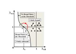
Figure 2: (Color online). The sketch of the typical stability diagram of a 3-body system in terms of couplings. The shaded area corresponds to stable systems, which have at least one bound state lying below the dissociation spectrum. The stability curve separates stable and unstable areas. A path connects the stable points lying very close the stability curve, whereby points 1 and 2 lie respectively above and below the critical point. The pictograms indicate the regions of Borromean, “‘tango”, “samba” and “all-bound” configurations. The change in the corner angle distribution along the path is illustrated in Fig. 3.

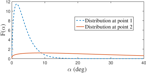
Figure 3: (Color online). Drastic change in the corner angle distribution $F(\alpha)$ when a point on the stability diagram travels along the path shown in Fig. 2. The path leading to such transition can be arbitrarily short.

We shall use the normalized Jacobi coordinates ${\boldsymbol{x}}=\hbar^{-1}\sqrt{m_{A}}({\boldsymbol{r}}_{2}-{\boldsymbol{r}}_{1})$ and ${\boldsymbol{y}}=\hbar^{-1}\sqrt{m_{A}m_{B}/(2m_{A}+m_{B})}(2{\boldsymbol{r}}_{3}-{\boldsymbol{r}}_{1}-{\boldsymbol{r}}_{2})$, where ${\boldsymbol{r}}_{i}$ are position vectors and particles $\{1,2\}$ are of type A, particle 3 is of type B. We shall always assume that $\int|\psi({\boldsymbol{x}},{\boldsymbol{y}})|^{2}d{\boldsymbol{x}}d{\boldsymbol{y}}=1$, where $\psi({\boldsymbol{x}},{\boldsymbol{y}})$ is the bound state wave function. On the stability curve the ground state energy equals the energy at the bottom of the continuum and regarding the behavior of energies and wave functions there are 3 possible scenarios my5 . If the system approaches the point on the stability curve, where $\lambda_{AA}<1$, its wave function does not spread my1 ; my2 ; my3 , the particles remain confined and for a point lying exactly on the stability curve there exists a well-defined normalized ground state wave function, which corresponds to zero energy. This exotic zero energy ground state wave function does not decay exponentially but rather falls off like an inverse polynomial my1 ; my3 . The second scenario is realized when the system approaches the stability curve, at the point where $\lambda_{AA}>1$. In that case the 3-body wave function $\psi({\boldsymbol{x}},{\boldsymbol{y}})$ totally spreads my1 and approaches a universal expression klaus ; my3 , namely,

$$\lim_{E\to 0}\left\|\psi({\boldsymbol{x}},{\boldsymbol{y}})-\frac{1}{4\pi}\phi_{AA}({\boldsymbol{x}})\frac{e^{-\sqrt{|E|}|{\boldsymbol{y}}|}}{|{\boldsymbol{y}}|}\right\|=0.$$ (2)

In Eq. (2) $E$ is the binding energy (energy of the bound state minus the energy of the lowest dissociation threshold) and $\phi_{AA}({\boldsymbol{x}})$ is the wave function of the bound pair $AA$ at the point, where the stability curve is hit. Suppose that the line $\lambda_{AA}=\textnormal{const}>1$ crosses the stability curve in the point where $\lambda_{AB}=\lambda_{AB}^{0}$. Let us denote by $E(\lambda_{AB})$ the energy of the stable system lying on the line $\lambda_{AA}=\textnormal{const}$. Then there is a constant c such that my5 ; klaus

$$\lim_{\lambda_{AB}\to\lambda_{AB}^{0}}cE(\lambda_{AB})(\lambda_{AB}-\lambda_{AB}^{0})^{-2}=1$$ (3)

The third scenario occurs when the stable system approaches the critical point along the line $\lambda_{AA}=1$. In this case my3

$$\lim_{E\to 0}\left\|\psi({\boldsymbol{x}},{\boldsymbol{y}})-\frac{\chi_{[1,\infty)}(\rho)}{\pi^{3/2}|\ln|E||^{1/2}}\frac{\bigl{\{}|{\boldsymbol{x}}|\sin(\sqrt{|E|}|{\boldsymbol{y}}|)+|{\boldsymbol{y}}|\cos(\sqrt{|E|}|{\boldsymbol{y}}|)\bigr{\}}e^{-\sqrt{|E|}|{\boldsymbol{x}}|}}{|{\boldsymbol{x}}|^{3}|{\boldsymbol{y}}|+|{\boldsymbol{y}}|^{3}|{\boldsymbol{x}}|}\right\|=0.$$ (4)

In Eq. (4) $\rho^{2}={\boldsymbol{x}}^{2}+{\boldsymbol{y}}^{2}$ and by definition $\chi_{[1,\infty)}(\rho)=1$ for $\rho\in[1,\infty)$ and $\chi_{[1,\infty)}(\rho)=0$ otherwise.

Let us denote by $E(\lambda_{AB})$ the energy of the stable system lying on the line $\lambda_{AA}=1$. Then there exists such constant $c$ that my5

$$\lim_{\lambda_{AB}\to\lambda_{cr}}cE(\lambda_{AB})\bigl{[}\ln(\lambda_{AB}-\lambda_{cr})\bigr{]}(\lambda_{AB}-\lambda_{cr})^{-1}=1,$$ (5)

where $\lambda_{cr}$ is the value of $\lambda_{AB}$ at the critical point. The same equation can be rewritten in terms of the scattering length

$$\lim_{a\to a_{cr}}c^{\prime}E(a)\bigl{[}\ln|a-a_{cr}|\bigr{]}(a-a_{cr})^{-1}=1,$$ (6)

where $a$ is the scattering length for the pair of pair of particles $AB$ interacting through $\lambda_{AB}V_{AB}$ and $a_{cr}$ is its value at the critical point and $c^{\prime}$ is another constant. Eq. (6) follows from Eq. (5) because $a_{cr}$ is finite and $a$ can be Taylor expanded in terms of the coupling constant. Eqs. (5)–(6) and Eqs. (2)–(4)hold universally, that is they are independent of the form of pair interactions. Eq. (4) was proved in my3 for the case when the critical point is approached along the line $\lambda_{AA}=1$. We do not prove it here but one can show that Eq. (4) holds true if the critical point is approached along any line within the stable part of the stability diagram. The argument largely resides on the fact the asymptotic of the binding energy deduced from Eq. (5) dominates over the asymptotic in Eq. (2).

If the 3-body system AAB is bound then from the underlying symmetries the ground state wave function can be written either as $\psi(\rho_{1},\rho_{2},\alpha)$ or $\psi(\rho_{1},x,\beta)$, where the corner angles $\alpha,\beta$ are illustrated in Fig. 1 and $\rho_{i}\equiv|{\boldsymbol{\rho}}_{i}|$, $x\equiv|{\boldsymbol{x}}|$. It is convenient to pass to the units, where $\hbar^{-1}\sqrt{m_{A}}=1$, in which case ${\boldsymbol{\rho}}_{2}-{\boldsymbol{\rho}}_{1}$ equals the Jacobi variable ${\boldsymbol{x}}$. Then one defines the corner angle distributions as follows

$$F(\alpha)=8\pi^{2}\kappa^{3}\sin\alpha\int_{0}^{\infty}\int_{0}^{\infty}\rho_{1}^{2}\rho_{2}^{2}|\psi(\rho_{1},\rho_{2},\alpha)|^{2}d\rho_{1}d\rho_{2},$$ (7)

$$\Phi(\beta)=8\pi^{2}\kappa^{3}\sin\beta\int_{0}^{\infty}\int_{0}^{\infty}\rho_{1}^{2}x^{2}|\psi(\rho_{1},x,\beta)|^{2}d\rho_{1}dx,$$ (8)

where we set $\kappa=2\sqrt{m_{B}/(m_{B}+2m_{A})}$. The ground state wave function written in coordinates ${\boldsymbol{x}},{\boldsymbol{y}}$ is normalized, as a result for corner angle distributions we get

$$\int_{0}^{\pi}F(\alpha)d\alpha=\int_{0}^{\pi}\Phi(\beta)d\beta=1.$$ (9)

(This is the reason for introducing the factor $8\pi^{2}\kappa^{3}$ in Eqs. (7)-(8)).

From Eqs. (2), (4) we see that the universal behavior in the vicinity of the critical point can be very different. Going around the critical point as shown in Fig. 2 causes a drastic change in the corner angle distributions. In Fig. 2 we move from the stable point that lies very close to the stability curve above the critical point to another stable point in the close proximity of the stability curve, which lies below the critical point. At the starting point the distribution has a delta-like shape that concentrates near $\alpha=0$ (for points exactly on the stability curve that lie above the critical point this distribution makes no sense). At the end point it becomes broad and at the critical point and for all points exactly on the stability curve that lie below the critical point it is well-defined. This bifurcation, which is shown in Fig. 3, is very similar to a phase transition in statistical physics. The path around the critical point leading to the “change of phase” in the sense of corner angle distributions can be arbitrarily short, which is in full analogy with phase transitions around the critical point in thermodynamics. And in full analogy with the physics of phase transitions there is a universal behavior associated with the critical point on the stability diagram.

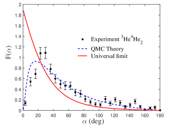
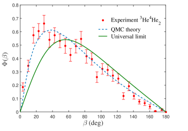
Figure 4: (Color online). Experimental and theoretical corner angle distributions in the asymmetric Helium trimer compared to the universal limits given by Eqs. (12)-(13), where $m_{A}/m_{B}=4/3$. The experimental data is taken from doerner2 , the quantum Monte Carlo calculation (QMC) was performed in bressanini . The area under all curves is equal to one.

If the critical point is approached along the line $\lambda_{AA}=1$ then

$$\lim_{\lambda_{AB}\to\lambda_{c}}\int_{0}^{\pi}|F(\alpha)-F_{c}(\alpha)|d\alpha=0,$$ (10)

$$\lim_{\lambda_{AB}\to\lambda_{c}}\int_{0}^{\pi}|\Phi(\beta)-\Phi_{c}(\beta)|d\beta=0,$$ (11)

where $F_{c}(\alpha)$ and $\Phi_{c}(\beta)$ and universal corer angle distributions at the critical point. Eqs. (10)-(11) hold also when the critical point is approached along the line lying in the stable area. In this paper we derive the explicit formulas for the universal corner angle distributions

$$F_{c}(\alpha)=\frac{4\left(1+\frac{2m_{A}}{m_{B}}\right)^{1/2}\sin\alpha}{\pi(1+\frac{m_{A}}{m_{B}})^{2}}I_{2}\left(\frac{\frac{m_{A}}{m_{B}}}{\frac{m_{A}}{m_{B}}+1},\cos\alpha\right),$$ (12)

$$\Phi_{c}(\beta)=\frac{\sin\beta}{\pi}\left(1+\frac{2m_{A}}{m_{B}}\right)^{1/2}I_{1}\left(\left(\frac{1}{2}+\frac{m_{A}}{2m_{B}}\right)^{1/2},\frac{\cos\beta}{2}\right)$$ (13)

Let us introduce the (discontinuous) function $g(x)=\arctan(x)$ for $x\geq 0$ and $g(x)=\pi-\arctan(|x|)$ for $x<0$. The following integrals depending on real parameters can be calculated analytically

$$I_{1}(s,b)=\int_{0}^{\infty}\frac{t^{2}dt}{(t^{2}-2bt+s^{2})^{2}}=\frac{b}{2(s^{2}-b^{2})}+\frac{s^{2}g(-\sqrt{s^{2}-b^{2}}/b)}{2(s^{2}-b^{2})^{3/2}}$$ (14)

$$I_{2}(s,b)=\int_{0}^{\infty}\frac{t^{2}dt}{(1+t^{2}-2tb)(t^{2}-2bst+1)^{2}}$$

$$=\frac{g(-\frac{\sqrt{1-b^{2}}}{b})}{4b^{2}\sqrt{1-b^{2}}(s-1)^{2}}+\frac{P_{1}(s,b)g(-\frac{\sqrt{1-s^{2}b^{2}}}{sb})+P_{2}(s,b)}{4b^{3}(1-s)^{4}(1-b^{2}s^{2})^{5/2}},$$ (15)

where

$$P_{1}(s,b)=(-2bs^{2}+5sb-4b)(1-s^{2}b^{2})^{2}+(3b-3bs+bs^{2}-b^{3}s)(1-b^{2}s^{2})$$

$$P_{2}(s,b)=(s-3-b^{2}+3b^{2}s)(1-s^{2}b^{2})^{3/2}+(3-s)(1-b^{2}s^{2})^{5/2}$$

The above integrals can be calculated using the following theorem: suppose that $\lambda>0$ is non-integer and the polynomial $Q(t)$ is non-zero for $t\geq 0$ and has degree larger than $1+\lambda$. Then

$$\int_{0}^{\infty}\frac{t^{\lambda-1}}{Q(t)}dt=\frac{\pi}{\sin(\lambda\pi)}\sum_{p}{\textnormal{Res}\>}_{p}\frac{(-z)^{\lambda-1}}{Q(z)},$$ (16)

where the sum is over the residues calculated in all poles of $Q(z)$ in the complex plain. To calculate the integrals in Eqs. (14)-(15) we apply his theorem by setting $\lambda=3+\epsilon$ and after that letting $\epsilon\to 0$. After the lengthy but straightforward calculation one obtains Eqs. (14)-(15).

Note one important feature regarding the universal corner angle distribution $F(\alpha)$. For any normalized wave function corresponding to a nonzero binding energy $F(0)=0$. Indeed, the wave function is finite and has an exponential fall off, therefore $F(0)=0$ results from the factor $\sin\alpha$ in Eq. (7). At the same time the universal limit for this distribution is such that $F_{c}(0)\neq 0$, on the contrary, $F_{c}(\alpha)$ reaches its maximum at zero. $F(\alpha)$ approaches $F_{c}(\alpha)$ in the sense of Eq. (10), but the convergence in the pointwise sense is nonuniform (this is also discussed in the remark on page 5 in my3 ). In the vicinity of the critical point $F(\alpha)$ starts from zero and goes steeply up staying close to the ordinate axis. Note also that the convergence to the universal limit with the vanishing binding energy is logarithmically slow. This follows from the logarithmic factor in the denominator in Eq. (4), which, in fact, eliminates nonuniversal components in the wave function my3 .

The asymmetric Helium trimer ³He⁴He₂ represents an example of a system that is close to the critical point on the stability diagram. The binding energy of this system is estimated to be 1.23$\times$10^-6 eV, which is very small on the atomic scale, the pair of atoms ³He₂ is unbound and the Helium dimer ⁴He₂ has the binding energy 1.14$\times$10^-7 eV, which is by an order of magnitude less than that of the trimer. This data suggests that the asymmetric Helium trimer lies very close to the critical point in the “tango” sector on the diagram in Fig. 2. The corner angle distributions for the asymmetric trimer were measured experimentally doerner2 . D. Bressanini doerner2 ; bressanini performed high precision Monte Carlo calculations of the asymmetric trimer using the TTY helium-helium potential hehepotential . Fig. 4 compares the experimental data and the calculations in bressanini with the universal limit given by Eqs. (12)-(13). Note that the area under all curves is equal to one. The data indicates that the corner angle distributions are relatively close to universal ones.

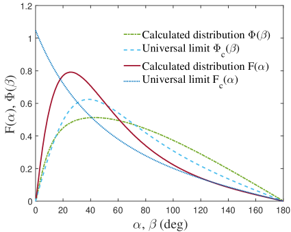
Figure 5: (Color online). Calculated corner angle distributions in the nucleus ²²C compared to the universal limits given by Eqs. (12)-(13), where $m_{A}/m_{B}=1/20$. The area under all curves is equal to one.

Another example of the system close to the critical point is the nucleus ²²C, which can be considered as a 3-body system consisting of the core ²⁰C and two neutrons forming a halo horiuchi ; vaagencarbon . This system lies in the Borromean square on the diagram in Fig. 2 because the nucleus ²¹C is unbound and two neutrons also do not form a bound pair. The available experimental data indicates carbonexp that the nucleus ²²C has an enormously large matter radius, the three-body calculation predicts the biding energy on the order of several KeV (compare this with the binding energy of the deutron 2 MeV, which is considered weakly bound on the nuclear scale). The two neutrons do not form a bound state but have a low lying virtual state at the energy about 143 KeV just above the threshold tomiocarbon . This suggests that being viewed as a 3-body system the nucleus ²²C lies in the Borromean sector rather close to the critical point.

We did the QMC calculation of the ²²C nucleus using cluster model used in vaagencarbon , which treats this nucleus as a three-body system consisting of 2 valence neutrons and the core. The neutrons interact with the core through the local potential having the Woods-Saxon shape vaagencarbon

$$V_{cn}(r)=-V_{0}\left[1+\exp(a^{-1}(r-R))\right]^{-1}$$ (17)

We use the same parameters used in vaagencarbon , namely, $a=0.6$ fm and $R=3.529$ fm. Like in vaagencarbon we tune the depth $V_{0}$ in order to reproduce the observed matter radius of the nucleus. The neutrons interact through the local Gaussian potential $V_{nn}(r)=-31\exp(-b^{-2}r^{2})$ (MeV), where $b=1.8$ fm. This interaction is tuned fedorovreports ; vaagencarbon ; vaagenreports in order to reproduce the low energy properties of the neutron-neutron system (among them the correct scattering length and no binding in the s channel). Though it is not explicitly mentioned, the neutron-neutron interaction used in vaagencarbon is nonlocal, it is set to zero in all partial waves except the $s$-wave. In the s-wave it is identical with the expression that is used here. Let us remark that for the low binding energy only low energy properties of the interaction matter. In particular, this is illustrated in Table II in vaagencarbon , where one can see that the weight of the components in the 3-body wave function for higher partial waves ($l_{x}\geq 1$) is less than 1%. Thus our model, where the local neutron-neutron interaction is nonzero in higher partial waves, is very similar to the one used in vaagencarbon . The technique of the QMC method is described in morozi .

In Eq. (17) we set the value $V_{0}=2.84$ MeV and obtain the separation energy of two neutrons $S_{2n}=0.0052(4)$ MeV and the mean squared hyperradius $\langle\rho^{2}\rangle=250(12)$ fm². According to Eq. (2) in vaagencarbon this gives $4.4$ fm for the root mean square matter radius, which is in accordance with the results listed in the Table I in vaagencarbon . In spite of very small binding energy this value is less than the mean value and nearly equals the lower bound for the experimental matter radius carbonexp . Fig. 5 compares the corner angle distribution for the calculated three-body wave function with the universal limits given by Eqs. (12)-(13). The deviation from the universal limit results from the finite scattering length in the neutron-neutron interaction.

Let us pass to the derivation of Eqs. (12)-(13). From Eqs. (3), (5) in my3 we know that when the critical point is approached

$$\int\rho^{5}|\psi(\rho,\theta,\hat{\boldsymbol{x}},\hat{\boldsymbol{y}})|^{2}d\rho\to\frac{1}{4\pi^{3}\cos^{2}\theta},$$ (18)

where $\rho^{2}={\boldsymbol{x}}^{2}+{\boldsymbol{y}}^{2}$, $\tan\theta=|{\boldsymbol{y}}|/|{\boldsymbol{x}}|$ and $\hat{\boldsymbol{x}},\hat{\boldsymbol{y}}$ are unit vectors in the directions of ${\boldsymbol{x}},{\boldsymbol{y}}$ respectively. Eq. (18) is the key point in the derivation. Note that with the chosen scales ${\boldsymbol{y}}=\kappa\tilde{\boldsymbol{y}}$, where the vector $\tilde{\boldsymbol{y}}$ is pictured in Fig. 1. In Eq. (8) let us change the integration variables from $x,\rho_{1}$ to $\rho,t$, where $t=\rho_{1}/x$. By a geometric argument (see Fig. 1 ) we get

$$\rho^{2}={\boldsymbol{x}}^{2}+\kappa^{2}{\tilde{\boldsymbol{y}}}^{2}=\left(1+\frac{\kappa^{2}}{4}\right)x^{2}+\kappa^{2}\rho_{1}^{2}-\kappa^{2}x\rho_{1}\cos\beta$$ (19)

Then the Jacobian of the transformation reads

$$J(\rho,t)=\begin{vmatrix}\frac{\partial\rho}{\partial x}&\frac{\partial\rho}{\partial\rho_{1}}\\ \frac{\partial t}{\partial x}&\frac{\partial t}{\partial\rho_{1}}\end{vmatrix}^{-1}=\rho\left[(1+\kappa^{2}/4)-\kappa^{2}t\cos\beta+\kappa^{2}t^{2}\right]^{-1}$$ (20)

We obviously have

$$x^{2}\rho_{1}^{2}=t^{2}x^{4}=t^{2}\rho^{4}\cos^{4}\theta$$ (21)

Thereby by Eq. (19)

$$\cos^{2}\theta=\frac{x^{2}}{\rho^{2}}=\frac{1}{(1+\kappa^{2}/4)-\kappa^{2}t\cos\beta+\kappa^{2}t^{2}}$$ (22)

Substituting Eq. (21) and Eq. (20) into Eq. (8) we obtain

$$\Phi(\beta)=8\pi^{2}\kappa^{3}\sin\beta\int_{0}^{\infty}\int_{0}^{\infty}t^{2}\rho^{4}\cos^{4}\theta|\psi(x(\rho,t),\rho_{1}(\rho,t),\beta)|^{2}J(\rho,t)d\rho dt$$ (23)

$$=8\pi^{2}\kappa^{3}\sin\beta\int_{0}^{\infty}dtt^{2}\cos^{6}\theta\int_{0}^{\infty}\rho^{5}|\psi(x(\rho,t),\rho_{1}(\rho,t),\beta)|^{2}d\rho.$$ (24)

Now we use Eq. (22) and Eq. (18) to get the expression for the critical corner angle distribution

$$\Phi_{c}(\beta)=\frac{2\kappa^{3}\sin\beta}{\pi}\int_{0}^{\infty}t^{2}\cos^{4}\theta dt=\frac{2\kappa^{3}\sin\beta}{\pi}\int_{0}^{\infty}\frac{t^{2}dt}{[(1+\kappa^{2}/4)-\kappa^{2}t\cos\beta+\kappa^{2}t^{2}]^{2}}$$ (25)

Substituting the expression for $\kappa$ in terms of masses we get Eq. (13). Now let us prove Eq. (12). In Eq. (7) let us change the integration variables from $\rho_{1},\rho_{2}$ to $\rho,t^{\prime}$, where $t^{\prime}=\rho_{2}/\rho_{1}$. From the geometry in Fig. 1

$$\rho^{2}={\boldsymbol{x}}^{2}+\kappa^{2}{\tilde{\boldsymbol{y}}}^{2}=(1+\kappa^{2}/4)(\rho_{1}^{2}+\rho_{2}^{2})-2\rho_{1}\rho_{2}(1-\kappa^{2}/4)\cos\alpha$$ (26)

For convenience let us introduce

$$\xi(t^{\prime},\alpha)=\left[(1+\kappa^{2}/4)(1+t^{\prime 2})-2(1-\kappa^{2}/4)t^{\prime}\cos\alpha\right]^{-1}$$ (27)

Now we can calculate the Jacobian of the transformation

$$J(\rho,t^{\prime})=\begin{vmatrix}\frac{\partial\rho}{\partial\rho_{1}}&\frac{\partial\rho}{\partial\rho_{2}}\\ \frac{\partial t^{\prime}}{\partial\rho_{1}}&\frac{\partial t^{\prime}}{\partial\rho_{2}}\end{vmatrix}^{-1}=\rho\xi(t^{\prime},\alpha).$$ (28)

Using Eq. (26) we also get

$$\rho_{1}^{2}\rho_{2}^{2}=\rho_{1}^{4}t^{\prime 2}=t^{\prime 2}\rho^{4}\left[\xi(t^{\prime},\alpha)\right]^{2}.$$ (29)

Eq. (22) can be rewritten as follows

$$\cos^{2}\theta=\frac{x^{2}}{\rho^{2}}=(1+t^{\prime 2}-2t^{\prime}\cos\alpha)\xi(t^{\prime},\alpha).$$ (30)

Passing to the new integration variables we get from Eq. (7)

$$F(\alpha)=8\pi^{2}\kappa^{3}\sin\alpha\int_{0}^{\infty}dt^{\prime}\left[\xi(t^{\prime},\alpha)\right]^{3}t^{\prime 2}\int_{0}^{\infty}\rho^{5}|\psi(\rho_{1}(\rho,t^{\prime}),\rho_{2}(\rho,t^{\prime}),\alpha)|^{2}d\rho$$ (31)

Hence, due to Eq. (30) and Eq. (18)

$$F_{c}(\alpha)=\frac{2\kappa^{3}\sin\alpha}{\pi}\int_{0}^{\infty}\frac{\left[\xi(t^{\prime},\alpha)\right]^{2}t^{\prime 2}}{1+t^{\prime 2}-2t^{\prime}\cos\alpha}dt^{\prime},$$ (32)

where one should substitute the explicit expression for $\xi(t^{\prime},\alpha)$ given by Eq. (27). After the substitution of $\kappa$ in terms of masses we get Eq. (12).

We thank S. Ershov, J. S. Vaagen, M. Zhukov, M. Kunitski and R. Dörner for stimulating discussions. One of us (D.G.) is grateful to Horst Stöcker for supporting the project at FIAS.

References

- (1) Braaten E, Hammer H-W (2006) Universality in few-body systems with large scattering length. Physics Reports 428: 259-390
- (2) Ferlaino F, Grimm R (2010) Trend: Forty years of Efimov physics: How a bizarre prediction turned into a hot topic. Physics 3:9
- (3) Kraemer T, Mark M, Waldburger P, Danzl J G, Chin C, Engeser B, Lange A D, Pilch K, Jaakkola A, Nägerl H-C, Grimm R (2006) Evidence for Efimov quantum states in an ultracold gas of caesium atoms. Nature 440: 315-318
- (4) B. Huang, L. A. Sidorenkov, R. Grimm, and J. M. Hutson: Observation of the Second Triatomic Resonance in Efimov’s Scenario, Phys. Rev. Lett. 112, 190401 (2014)
- (5) Knoop S, Ferlaino F, Mark M, Berninger M, Schöbel H, Nägerl H-C, Grimm R (2009) Observation of an Efimov-like trimer resonance in ultracold atomdimer scattering. Nature Phys. 5: 227-230
- (6) Zaccanti M, Deissler B, D’Errico C, Fattori M, Jona-Lasinio M, Müller S, Roati G, Inguscio M, Modugno G (2009) Observation of an Efimov spectrum in an atomic system. Nature Phys. 5: 586-591
- (7) Gross N, Shotan Z, Kokkelmans S, Khaykovich L (2009) Observation of Universality in Ultracold 7Li Three-Body Recombination. Phys. Rev. Lett. 103: 163202
- (8) Pollack S E, Dries D, Hulet R G (2009) Universality in Three- and Four-Body Bound States of Ultracold Atoms. Science 326: 1683-1685
- (9) Ottenstein T B, Lompe T, Kohnen M, Wenz A N, Jochim S (2008) Collisional Stability of a Three-Component Degenerate Fermi Gas. Phys. Rev. Lett. 101: 20320
- (10) Huckans J H, Williams J R, Hazlett E L, Stites R W, O’ Hara K M (2009) Three-Body Recombination in a Three-State Fermi Gas with Widely Tunable Interactions. Phys. Rev. Lett. 102: 165302
- (11) Williams J R, Hazlett E L, Huckans J H, Stites R W, Zhang Y, O’Hara K M (2009) Evidence for an Excited-State Efimov Trimer in a Three-Component Fermi Gas. Phys. Rev. Lett. 103: 130404
- (12) Wenz A N, Lompe T, Ottenstein T B, Serwane F, Zürn G, Jochim S (2009) Universal trimer in a three-component Fermi gas. Phys. Rev. A 80: 040702(R)
- (13) Lompe T, Ottenstein T B, Serwane F, Wenz A N, Zürn G, Jochim S (2010) Radio-Frequency Association of Efimov Trimers. Science 330: 940-944
- (14) Efimov V (1970) Energy levels arising from resonant two-body forces in a three-body system. Phys. Lett.B 33: 563-564; Sov. J. Nucl. Phys. 12, 589 (1971)
- (15) Yusuke Nishida, Sergej Moroz, and Dam Thanh Son: Super Efimov Effect of Resonantly Interacting Fermions in Two Dimensions, Phys. Rev. Lett. 110, 235301 (2013)
- (16) D. K. Gridnev: Three resonating fermions in flatland: proof of the super Efimov effect and the exact discrete spectrum asymptotics, J. Phys. A: Math. Theor. 47 505204 (2014)
- (17) Kunitski M, Zeller S, Voigtsberger J, Kalinin A, Schmidt, L P H Sch ̵̈offler M, Czasch A, W. Schöllkopf W, Grisenti R E, Jahnke T, Blume D, Dörner R (2015) Observation of the Efimov state of the helium trimer. Science 348:551-555
- (18) Voigtsberger J, Zeller S, Becht J, Neumann N, Sturm F, Kim H-K, Waitz M, Trinter F, Kunitski M, Kalinin A, Wu J, Schöllkopf W, Bressanini D, Czasch A, Williams J B, Ullmann-Pfleger K, Schmidt L P H, Schöffler M S, Grisenti R E, Jahnke T, Dörner R Imaging the structure of the trimer systems 4He3 und 3He4He2, Nat. Commun. 5, 5765 (2014)
- (19) Zhukov, M.V., Danilin, B.V., Fedorov, D.V., Bang, J.M., Thompson, I.J., Vaagen, J.S.: Bound state properties of Borromean halo nuclei 6He 11Li Phys. Rep. 231, 151-199 (1993)
- (20) Tanaka et al.: Observation of a Large Reaction Cross Section in the Drip-Line Nucleus 22C, Phys. Rev. Lett. 104, 062701 (2010)
- (21) Ershov, S.N., Vaagen, J.S., Zhukov, M.V.: Binding energy constraint on matter radius and soft dipole excitations of 22C, Phys. Rev. C 86, 034331-034338 (2012)
- (22) W. Horiuchi and Y. Suzuki: 22C: An s-wave two-neutron halo nucleus, Phys. Rev. C 74, 034311-034316 (2006).
- (23) L. A. Souza, F. F. Bellotti, T. Frederico, M. T. Yamashita, L. Tomio, Scaling limit analysis of Borromean halos, arXiv:1603.03407 [nucl-th]
- (24) D. Bressanini and G. Morosi, J Phys Chem A. 115, 10880-7 (2011).
- (25) J.-M. Richard and S. Fleck: Limits on the Domain of Coupling Constants for Binding N-Body Systems with No Bound Subsystems, Phys. Rev. Lett. 73, 1464 (1994)
- (26) P.G. Hansen and B. Jonson: The Neutron Halo of Extremely Neutron-Rich Nuclei, Europhys. Lett. 4 (1987) 409.
- (27) A.S. Jensen, K. Riisager, D.V. Fedorov, E. Garrido, Classification of three-body quantum halos, Europhys.Lett.61:320-326, (2003)
- (28) M. T. Yamashita, T. Frederico, L. Tomio: Spatial characteristics of borromean, tango, samba and all-bound halo nuclei, AIP Conf. Proc. 884(2007) pp.129-134
- (29) D. K. Gridnev: Zero-energy bound states and resonances in three-particle systems, J. Phys. A: Math. Theor. 45 175203 (2012)
- (30) D. K. Gridnev: Zero energy bound states in many–particle systems, J. Phys. A: Math. Theor. 45 395302 (2012)
- (31) D. K. Gridnev: Universal angular probability distribution of three particles near zero-energy threshold, J. Phys. A: Math. Theor. 46 115204 (2013)
- (32) D. K. Gridnev: Universal low-energy behavior in three-body systems, J. Math. Phys. 56, 022107 (2015)
- (33) B. Simon and M. Klaus: Coupling constant thresholds in nonrelativistic quantum mechanics. II. Two-cluster thresholds in N-body systems, Comm. Math. Phys. 78, (2) (1980), 153-168.
- (34) D. Bressanini: The Structure of the Asymmetric Helium Trimer 3He4He2, J. Phys. Chem. A, 2014, 118 (33), pp 6521–6528
- (35) Tang, K. T.; Toennies, J. P.; Yiu, C. L. Accurate analytical He−He van der Waals potential based on perturbation theory. Phys. Rev. Lett. 1995, 74 (9), 1546−9
- (36) D. V. Fedorov, A. S. Jensen, and K. Riisager, Efimov States in Halo Nuclei, Phys. Rev. Lett. 73, 2817-2820 (1994)