A full, self-consistent, treatment of thermal wind balance on oblate fluid planets

(Journal of Fluid Mechanics - under revision - July 2016)

Abstract

The nature of the flow below the cloud level on Jupiter and Saturn is still unknown. Relating the flow on these planets to perturbations in their density field is key to the analysis of the gravity measurements expected from both the Juno (Jupiter) and Cassini (Saturn) spacecrafts during 2016-18. Both missions will provide latitude-dependent gravity fields, which in principle could be inverted to calculate the vertical structure of the observed cloud-level zonal flow on these planets. Theories to date connecting the gravity field and the flow structure have been limited to potential theories under a barotropic assumption, or estimates based on thermal wind balance that allow analyzing baroclinic wind structures, but have made simplifying assumptions that neglected several physical effects. These include the effects of the deviations from spherical symmetry, the centrifugal force due to density perturbations, and self-gravitational effects of the density perturbations. Recent studies attempted to include some of these neglected terms, but lacked an overall approach that is able to include all effects in a self-consistent manner. The present study introduces such a self-consistent perturbation approach to the thermal wind balance that incorporates all physical effects, and applies it to several example wind structures, both barotropic and baroclinic. The contribution of each term is analyzed, and the results are compared in the barotropic limit to those of potential theory. It is found that the dominant balance involves the original simplified thermal wind approach. This balance produces a good order-of-magnitude estimate of the gravitational moments, and is able, therefore, to address the order one question of how deep the flows are given measurements of gravitational moments. The additional terms are significantly smaller yet can affect the gravitational moments to some degree. However, none of these terms is dominant so any approximation attempting to improve over the simplified thermal wind approach needs to include all other terms.

1 Introduction

The observed cloud-level flow on Jupiter and Saturn is dominated by strong east-west (zonal) flows. The depth to which these flows extend is unknown, and has been a topic of great debate over the past few decades (see reviews by Vasavada and Showman,, 2005 and Showman et al.,, 2016). One of the prime goals of the Juno mission to Jupiter and the Cassini Grande Finale at Saturn is to estimate the depth of these flows via precise gravitational measurements. If the flows are indeed deep, and therefore perturb significant mass, then they can produce a gravity signal that will be measurable (Hubbard,, 1999; Kaspi et al.,, 2010). Constraining the depth of these flows will help explore the mechanisms driving the jets (e.g., Busse,, 1976; Williams,, 1978; Ingersoll and Pollard,, 1982; Cho and Polvani,, 1996; Showman et al.,, 2006; Scott and Polvani,, 2007; Kaspi and Flierl,, 2007; Lian and Showman,, 2010; Liu and Schneider,, 2010; Heimpel et al.,, 2016), and give better constraints on interior structure models (e.g., Guillot,, 2005; Militzer et al.,, 2008; Nettelmann et al.,, 2012; Helled and Guillot,, 2013).

Several studies over the past decades have examined the effects of interior flow on the gravitational moments. The gravity moment spectrum mostly results from the planet’s oblate shape due to its rotation, and from the corresponding interior density distribution. However, density perturbations due to atmospheric dynamics and internal flows can affect the measured gravity moments especially if the flows extend deep enough into the planets. Hubbard, (1982) and Hubbard, (1999) used potential theory to calculate the gravity moments due to internal flows, by extending the observed cloud-level winds along cylinders throughout the planet as suggested by Busse, (1976). This approach takes into account the oblateness of the planet, yet is only possible for the barotropic case, meaning that the flow is constant along lines parallel to the axis of rotation. This occurs if the baroclinicity vector $\nabla\rho\times\nabla p$ vanishes (e.g., if density is a function of pressure only) at small Rossby number and negligible dissipation. More recently, Hubbard introduced more accurate calculations, for the gravitational signature of the flows (Hubbard,, 2012; Kong et al.,, 2012; Hubbard,, 2013), using concentric Maclaurin spheroids (CMS), but these are also only limited to the fully barotropic case.

A different approach, assuming the large scale flow is dominated by the rotation of the planet, used thermal wind balance to calculate the gravity moments due to the wind field (Kaspi et al.,, 2010; Kaspi,, 2013; Kaspi et al.,, 2013; Liu et al.,, 2013, 2014). The thermal wind approach is not limited to the barotropic case (can account for any wind field), and in the barotropic limit has been shown to be equivalent to the potential theory and CMS methods (Kaspi et al.,, 2016). In addition, this approach allows for the calculation of the odd gravitational moments, which can emerge from north-south hemispherical asymmetries in the wind structure (Kaspi,, 2013). However, this thermal wind approach was originally limited to spherical symmetry, resulting in an inability to calculate the effects of the planet oblateness on the gravity signature of the winds. Cao and Stevenson, (2015) added the effects of oblateness on the background state density and gravity and concluded that it should be considered when estimating the effects of the winds on the gravity moments using thermal-wind. Similarly, Zhang et al., (2015) included another effect, of the gravity anomalies due to density perturbations associated with the winds, and found an effect on the second gravity moment $J_{2}$, terming their approach thermal-gravity wind (TGW) method. However, while both of these recent studies found some effects of the terms they added, their choice of added physics did not result from a systematic and self-consistent approach.

The purpose of this study is to develop a full, self-consistent thermal wind (FTW) perturbation approach for the treatment of the general thermal wind balance on a fluid planet. This will allow to calculate density anomalies and gravity moments due to prescribed winds, omitting the traditional sphericity assumptions which have been adopted from dynamics on terrestrial planets. Our approach includes the effect of oblateness, as well as that of gravity anomalies due to the dynamical density perturbations themselves. We show these two effects to be but two of several different factors that should be considered in a self-consistent calculation. Our approach is based on a systematic perturbation expansion, which both allows us to consider all effects, and also points the way to improving the estimated gravity moments using a higher order perturbation that can be considered by future studies.

By including all relevant terms in the general thermal wind balance, we are able to evaluate the relative contribution of different terms. We find that the simplified thermal wind (TW) approach captures most of the relation between the wind shear and density gradients. The term added in TGW is found to be one of several smaller terms that all need to be added together for consistency in order to improve the estimates of the simplified thermal wind balance. Furthermore, previous applications of the thermal wind balance encountered an unknown integration constant that was a function of radius only and could not be solved for. We show that this integration constant may have an effect, although small, on the gravity moments, and develop a method for calculating it.

The following section describes the perturbation approach, the resulting equations and how they are solved. Next, in section 3, we first verify this approach by comparing it to the results of the CMS method in the barotropic limit, and then compare our results to the less complete approaches of simplified thermal wind and TGW. We then also apply the self-consistent solution to a case with baroclinic winds where CMS cannot be used. We discuss the results and conclude in section 4.

2 Methods: perturbation expansion of the momentum equations

We begin by taking the standard form of the momentum equations on a planet rotating at an angular velocity $\Omega$,

$$\frac{\partial\mathbf{u}}{\partial t}+\left(\mathbf{u\cdot\nabla}\right)\mathbf{u}+2\boldsymbol{\Omega}\times\mathbf{u}+\boldsymbol{\Omega}\times\boldsymbol{\Omega}\mathbf{\times r} = -\frac{1}{\rho}\nabla p+\nabla\Phi,$$ (1)

where $\mathbf{u}$ is the 3D wind vector, $\rho$ is density, $p$ is pressure, $\boldsymbol{\Omega}$ is the planetary rotation rate, and $\Phi$ is the body force potential. The first term on the lhs is the local acceleration of the flow, the second is the Eulerian advection, the third is the Coriolis acceleration, and the fourth is the centrifugal acceleration. On right hand side appear the pressure gradient term and the body force (gravity in this case, so that $\nabla\Phi={\bf-g}$). Note that by gravity we refer here to the force due to the Newtonian potential, not to the modified gravity which is commonly used in geostrophic studies and includes the centrifugal potential as well. Typical values for a Jupiter-like planet are $U=O\left(100\right)$ m s^-1, $\Omega=O\left(10^{-4}\right)$ s^-1, $a=O\left(7\times 10^{7}\right)$ m, where $a$ is the planet radius. The resulting Rossby number ($Ro$) is therefore much smaller than one ($Ro\equiv U/\Omega a\thickapprox 10^{-2}$), and as the first two terms in Eq. 1 can be neglected so that the resulting balance is,

$$2\boldsymbol{\Omega}\mathbf{\times\left(\rho u\right)} = -\nabla p-\rho{\bf g}-\rho\boldsymbol{\Omega}\times\boldsymbol{\Omega}\mathbf{\times r}.$$ (2)

Next, we denote the static solution ($\mathbf{u}=0$) as $\rho_{0},p_{0},g_{0}$, and the perturbations due to the non zero wind (dynamical part of the solution) as $\rho^{\prime},p^{\prime},g^{\prime}$, such that

$$\rho = \rho_{0}(r,\theta)+\rho^{\prime}(r,\theta),$$

$$p = p_{0}(r,\theta)+p^{\prime}(r,\theta),$$

$${\bf g} = {\bf g}_{0}(r,\theta)+{\bf g}^{\prime}(r,\theta).$$ (3)

Note that both the static and the dynamic solutions are functions of latitude and radius, and that the gravity is directly related to the density via a relation shown below.

The equation obtained by setting the small Rossby number to zero as a first approximation is effectively static and does not include the velocity field,

$$0 = -\nabla p_{0}-\rho_{0}g_{0}-\rho_{0}\boldsymbol{\Omega}\times\boldsymbol{\Omega}\mathbf{\times r},$$ (4)

and the dynamical perturbations therefore satisfy,

$$2\boldsymbol{\Omega}\mathbf{\times\left(\rho_{0}u\right)} = -\nabla p^{\prime}-\rho_{0}{\bf g}^{\prime}-\rho^{\prime}{\bf g}_{0}-\rho^{\prime}\boldsymbol{\Omega}\times\boldsymbol{\Omega}\mathbf{\times r}.$$ (5)

The solution procedure outlined here involves first finding the static solution and then solving Eq. 5 for the dynamical perturbations to the density due to the effects of the prescribed winds. Taking the curl of Eq. 5 yields a single equation in the azimuthal direction

$$-2\Omega r\partial_{z}\left(\rho_{0}u\right) = -rg_{0}^{(\theta)}\frac{\partial\rho^{\prime}}{\partial r}-g_{0}^{(r)}\frac{\partial\rho^{\prime}}{\partial\theta}+r\frac{\partial\rho_{0}}{\partial r}g^{\prime}{}^{(\theta)}-g^{\prime(r)}\frac{\partial\rho_{0}}{\partial\theta}\Omega^{2}r\left[\frac{\partial\rho^{\prime}}{\partial\theta}\cos^{2}\theta+\frac{\partial\rho^{\prime}}{\partial r}r\cos\theta\sin\theta\right],$$ (6)

where the notation $\partial_{z}=\cos\theta\frac{\partial}{\partial r}-\sin\theta\frac{\partial}{\partial\theta}$ denotes the derivative along the direction of the axis of rotation ($z$), and gravity is expressed as function of the density as,

$$\mathbf{g}(r,\theta)\mathbf{=}2\pi G\left[\frac{\partial}{\partial r},\frac{\partial}{r\partial\theta}\right]\iint\left\langle\frac{1}{|\mathbf{r-}\mathbf{r}^{\prime}|}\right\rangle\mathbf{\rho}(r^{\prime},\theta^{\prime})r^{\prime 2}\cos\theta^{\prime}d\theta^{\prime}dr^{\prime}$$ (7)

where the gravity can be either $\mathbf{g_{0}}$ or $\mathbf{g^{\prime}}$, calculated from $\rho_{0}$ or $\rho^{\prime}$, respectively, and $G=6.67\times 10^{-11}$ m³ kg${}^{-1}\,$ s^-2 is the gravitational constant. Note that Eq. 6, together with Eq. 7, form an integro-differential equation whose solution requires the calculation of integration constants as is done below and demonstrated in a simpler context in Appendix B.

Figure 1: The static model solution, as function of radius and latitude, from the CMS model for the density and gravity (panels a-c), and their deviation from the latitudinal mean (panels d-f).

The above equations for the perturbation density are the first order perturbation equations, which are solved in this study. It is important to note, though, that because this is a self-consistent treatment of the density perturbations, it also allows improving on the approximation by proceeding to the next orders. As a demonstration, we write the second order perturbation equations in Appendix A.1.

2.1 The background static solution

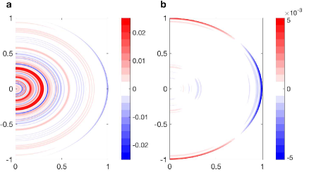
The static density $\rho_{0}$ and gravity $\mathbf{g_{0}}$ are taken from the solution of the CMS model (Hubbard,, 2012, 2013). The model is based on a numerical method for solving the equilibrium shape of a rotating planet, for which an analytic solution exists in the form of a Maclaurin spheroid. The continuously varying density and pressure structures are represented by a discrete set of layers, in which the density and pressure are constant. This onion-like structure is then decomposed into a set of concentric Maclaurin spheroids, and a solution is sought for by requiring that the sum of the gravitational potential and the rotational potential are constant on the surface of the planet (Hubbard,, 2012, 2013). Solutions using this method give similar results to other methods (Wisdom and Hubbard,, 2016; Kaspi et al.,, 2016). The static fields resulting from the CMS solution are shown in Fig. 1. Both the density and gravity fields show a structure that is mostly radial. While the density (Fig. 1a) ranges from zero to about 4000 kg m^-3, its latitude-dependent component (Fig. 1d) ranges only between -150 and 100 kg m^-3. Similarly, the radial gravity is also dominated by its radial component (Fig. 1b,e), with the peak gravity being $\sim 32$ m s^-2 at about $0.7a$. The latitudinal component of the gravity is much weaker than the radial component (Fig. 1c,f). Comparing panels c and f, shows that the latitudinal mean of the latitudinal component of the gravity is zero, and has a much smaller magnitude than the radial component. Note that in Fig. 1c,f a positive value means gravity pointing northward.

2.2 Solving for the dynamic density perturbations

We solve Eq. 6 by writing the equations in matrix form (e.g., Zhang et al.,, 2015). The 2D problem (radius and latitude) is discretized in both directions, where $N_{r}$ and $N_{\theta}$ are the number of grid points in radius and latitude, respectively. $N=N_{r}\times N_{\theta}$ is the total number of grid points. Equation 6 is then written in matrix form,

$$b = A\rho^{\prime},$$ (8)

where $A$ is a $N\times N$ matrix with contributions from all terms in the $rhs$ of the equation, $b$ is the known $lhs$ of the equation, due to the prescribed wind field, written an a $N\times 1$ vector, and the unknown density perturbation $\rho^{\prime}$ is written as a $N\times 1$ vector. All partial derivatives are written in center finite difference form, aside from near the boundaries where the derivatives are evaluated between grid points and weighted together with the adjacent derivative. Note that the gravity is fully calculated in the matrix (Eq. 8). It is done explicitly for each grid point.

Solving Eq. 8 involves the inversion of the matrix $A$, which is not possible because the matrix is singular and thus has a null space, which leads to a part of the solution that cannot be determined from the equation. This can be better understood in the simpler case where equation 6 is reduced to the thermal wind balance with a spherical base state, involving only the lhs and the second term on the rhs. In that case, the equation can be integrated in latitude, leaving an unknown integration constant that is a function of radius alone (e.g., Kaspi et al.,, 2010). In the more general case solved here, while the base state is a function of both radius and latitude, the null space still has a dimension equal to the number of radial grid points $N_{r}$, similar to the unknown function of radius only, but which has latitudinal dependence as well. We show in Appendix A.2 how the integration constant is calculated analytically in the simpler case, and discuss below (section 2.3) the solution in the more general case. In order to solve for the non-null part of the solution, we use singular value decomposition as follows. Let

$$A=U\Sigma V^{T},$$

where $U$ and $V$ are unitary matrixes, and $\Sigma$ is a rectangular diagonal matrix, then the pseudo inverse of $A$ is given by

$$A^{\dagger}=V\Sigma^{\dagger}U^{T},$$

where

$$\Sigma = diag(\sigma_{1},\ldots,\sigma_{N-N_{r}},0,\ldots,0),$$

$$\Sigma^{\dagger} = diag(\sigma_{1}^{-1},\ldots,\sigma_{N-N_{r}}^{-1},0,\ldots,0)\text{.}$$

The solution is now written as $\rho^{\prime}=\hat{\rho}^{\prime}+\delta\rho^{\prime}$, such that $\hat{\rho}^{\prime}$ is the part obtained from the pseudo inverse,

$$\hat{\rho}^{\prime}=A^{\dagger}b,$$

and the additional component $\delta\rho^{\prime}$ is in the null space of $A$, so that $A\rho^{\prime}=A(\hat{\rho}^{\prime}+\delta\rho^{\prime})=A\hat{\rho}^{\prime}=b$. That is, denoting the eigenvectors of $A$ by $\mathbf{e}_{i}$, such that $A\mathbf{e}_{i}=\lambda_{i}\mathbf{e}_{i}$, then the null space of the solution corresponds to any linear combination of eigenvectors corresponding to the zero eigenvalues, which may be added to the solution $\hat{\rho^{\prime}}$ while still satisfying $A\rho^{\prime}=b$. We next discuss the calculation of the null space and its contribution to the solution for $\rho^{\prime}$.

2.3 Calculating the null-space solution

As mentioned above, the number of null eigenvalues is always found to be $N_{n}=N_{r}$, i.e., equal to the number of grid points in the radial direction, hinting to the possibility that the modes are predominantly radially dependent. Indeed, looking at the zero eigenvectors does show this characteristic (see example in Fig. 2a). Nevertheless, since the null eigenvectors do depend on latitude (Fig. 2b), and this dependence is concentrated close to the planet upper levels, it could have a substantial effect on the gravity moments. The contribution of the null space to the density may be written as,

$$\delta\rho^{\prime} = \sum_{i=N-N_{r}+1}^{N}c_{i}\mathbf{e}_{i}=E\mathbf{c},$$ (9)

where $E$ is a $N\times N_{n}$ matrix whose columns are the $N_{n}$ null eigenvectors, and $\mathbf{c}$ is a $N_{n}\times 1$ vector of the unknown amplitudes of the null eigenvectors. In order to calculate the vector $\mathbf{c}$, we must introduce additional physics in the form of the polytropic relation between the pressure and the density (a demonstration of a full analytical solution using the polytropic equation is shown in Appendix A.2 for a simpler case). An additional constraint will be the conservation of the total mass of the planet. Note that the polytropic relation is only used for the solution of the null space, but the rest of the solution is independent of it.

Figure 2: An example of a null mode $V$. (a) the full null model, (b) the latitudinal dependent part of the null mode ($V_{a}=V-\overline{V})$. Note that in most of the domain, the structure of the mode depends on radius only, aside from the region close to the surface where a large scale latitude dependent structure exists, but whose value is around half the magnitude of the full structure.

The polytropic equation, $p=K\rho^{2}$, linearized around the static solution, gives

$$p^{\prime}=Kn\rho_{0}\rho^{\prime},$$ (10)

which may be used to define $\hat{p}^{\prime}$ as

$$\hat{p}^{\prime}\equiv Kn\rho_{0}\hat{\rho}^{\prime}.$$ (11)

Previously we took the curl of the momentum equation (Eq. 5), to solve for $\hat{\rho}^{\prime}(r,\theta)$, and it satisfies the original equation up to a gradient of some scalar function $\psi$. We therefore may replace the pressure $\hat{p}^{\prime}$ with $\hat{p}^{\prime}+\psi$. Using this augmented function, the perturbation momentum equation may be written as,

$$2\boldsymbol{\Omega}\mathbf{\times u}\rho_{0}=-\nabla(\hat{p}^{\prime}+\psi)-\rho_{0}\mathbf{\hat{g}}^{\prime}-\hat{\rho}^{\prime}\mathbf{g}_{0}-\hat{\rho}^{\prime}\boldsymbol{\Omega}\times\boldsymbol{\Omega}\mathbf{\times r}.$$ (12)

Next, taking the difference between the momentum equation for $\rho^{\prime}$ and for $\hat{\rho}^{\prime}$, we find,

$$0=-\nabla(p^{\prime}-\hat{p}^{\prime}-\psi)-\rho_{0}\mathbf{\delta g}^{\prime}-\delta\rho^{\prime}\mathbf{g}_{0}-\delta\rho^{\prime}\boldsymbol{\Omega}\times\boldsymbol{\Omega}\mathbf{\times r}.$$ (13)

The function $\psi$ appears as a correction to the perturbation pressure, and we therefore define the perturbation pressure to be,

$$\delta p^{\prime}\equiv p^{\prime}-\hat{p}^{\prime}-\psi.$$

Taking the difference between the polytropic equation for $\rho$ and $\hat{\rho}^{\prime}$, we have

$$\delta p^{\prime}=Kn\rho_{0}\delta\rho^{\prime},$$

which leads to an equation for the unknown perturbation density,

$$0=-\nabla(Kn\rho_{0}\delta\rho^{\prime})-\rho_{0}\mathbf{\delta g}^{\prime}-\delta\rho^{\prime}\mathbf{g}_{0}-\delta\rho^{\prime}\boldsymbol{\Omega}\times\boldsymbol{\Omega}\mathbf{\times r},$$ (14)

and explicitly,

$$F_{r}:\,\,\,\,\,\,0 = -2K\frac{\partial}{\partial r}(\rho_{0}\delta\rho^{\prime})-\rho_{0}\mathbf{\delta}g^{\prime(r)}-\delta\rho^{\prime}g_{0}^{(r)}+\delta\rho^{\prime}\Omega^{2}r\cos^{2}\theta,$$

$$F_{\theta}:\,\,\,\,\,\,0 = -2K\frac{\partial}{r\partial\theta}(\rho_{0}\delta\rho^{\prime})-\rho_{0}\mathbf{\delta}g^{\prime(\theta)}-\delta\rho^{\prime}g_{0}^{(\theta)}-\delta\rho^{\prime}\Omega^{2}r\cos\theta\sin\theta,$$

where $F_{r}$ and $F_{\theta}$ are the equations in the radial and latitudinal directions, respectively. This represents the radial and latitudinal components of a vector equation, and we next take the divergence to get a single equation,

$$0 = \frac{1}{r^{2}}\frac{\partial}{\partial r}(r^{2}F_{r})+\frac{1}{r\sin\theta}\frac{\partial}{\partial\theta}(\sin\theta F_{\theta}),$$ (15)

where everything but $\delta\rho^{\prime}$ is known. Numerically, this equation can be written as a set of linear equations,

$$B\delta\rho^{\prime} = 0,$$

where $B$ is a $N\times N$ matrix, and the rhs is a $N\times 1$ vector with zeros in all entries. An additional constraint is that the total mass of the planet must not change due to the existence of the wind, so that $\int\rho^{\prime}d^{3}\mathbf{r}=0$ and therefore,

$$\int\delta\rho^{\prime}d^{3}\mathbf{r}=-\int\hat{\rho}^{\prime}d^{3}\mathbf{r}=-\delta M.$$ (16)

The mass $\delta M$, due to the non-null space solution $\hat{\rho}^{\prime}$, is known from the solution to Eq. 6. Adding this constraint to Eq. 15 results in augmenting the matrix $B$ with an additional row, to form a matrix $\tilde{B}$ whose size is now $(N+1)\times N$ and the rhs, now denoted $\mathbf{m}$, is now a vector of length $N+1$ with a nonzero value only in the last entry, $m_{N+1}=-\delta M$. Using the definition for the null space part of the solution (9) we get,

$$\tilde{B}E\mathbf{c} = \mathbf{m}.$$

This is a formally overdetermined problem, which is solved for $\mathbf{c}$ using least squares (Strang,, 2006), allowing us to then calculate $\delta\rho^{\prime}$. Note that even though $\tilde{B},E$ and $\mathbf{m}$ are all complex, $\delta\rho^{\prime}$ is found to be real, as expected.

The use of a polytropic relation between the pressure and density implies that the baroclinic vector $\nabla p\times\nabla\rho$ vanishes, and therefore that the velocity field is necessarily barotropic at small Rossby numbers. This is in line with most of the cases discussed here that are indeed barotropic, aside from the last case that is baroclinic and is analyzed in section 3.3. Note that a different pressure-density relation is also possible. Nonetheless, in all cases discussed here the contribution of the null space solution to the overall solution is negligible. Our purpose here is to show how adding information regarding the equation of state (in this case $p(\rho)$) can be used to calculate the unknown integration constant arising in the thermal wind formulation (e.g., Kaspi et al.,, 2010; Zhang et al.,, 2015). However, in future application, one would need to use a more realistic equation of state that allows for determining the null space for a baroclinic wind field as well.

2.4 Prescribed winds

The wind profile used in this study is based on the measured cloud-tracking wind during the Cassini flyby (Porco et al.,, 2003). Since we compare our results to the CMS model solution as a reference for the full oblate solution, and the CMS wind profile must be truncated for numerical convergence (see Kaspi et al., (2016) for details), we use a 24th degree expansion of its differential potential. Kaspi et al., (2016) shows a comparison between the resulting gravity moments using the truncated and untruncated wind profiles. The choice of the specific wind profile does not affect the results. In order to do a proper comparison to the CMS model, which is limited to barotropic winds, the wind profile is extended along cylinders parallel to the direction of the axis of rotation. For the baroclinic case discussed in (section 3.3), the wind profile is extended toward the interior using an exponential decay function (e.g., as in Galanti and Kaspi, 2016a, ) with a decay scale height of $1000$ km.

2.5 Calculating gravity moments

In all cases discussed below, in addition to examining the solution for the density perturbations, we calculate the resulting gravitational moments given by

$$\Delta J_{n}=-\frac{2\pi}{Ma^{n}}\intop_{0}^{a}r^{\prime n+2}dr^{\prime}\intop_{-1}^{1}P_{n}\left(\mu^{\prime}\right)\rho^{\prime}\left(r^{\prime},\mu^{\prime}\right)d\mu^{\prime},$$ (17)

where $M$ is the mass of the planet, $P_{n}$ are the Legendre polynomials, and $\mu=\cos(\theta)$. Note that any part of $\rho^{\prime}$ that is a function of radius only does not contribute to the gravity moments. For instance, using the latitudinal average of the density, $\rho^{\prime}_{m}(r)=\overline{\rho^{\prime}(r,\theta)}$ in Eq. 17 will give

$$\Delta J_{n}=-\frac{2\pi}{Ma^{n}}\intop_{0}^{a}r^{\prime n+2}\rho^{\prime}_{m}\left(r^{\prime}\right)dr^{\prime}\intop_{-1}^{1}P_{n}\left(\mu^{\prime}\right)d\mu^{\prime}=0,$$ (18)

which vanishes due to the Legendre polynomials having a zero latitudinal mean for any value of $n$. Therefore, any solution for $\rho^{\prime}$ needs to be examined with respect to its latitudinal dependent part.

3 Results for wind-induced density and gravity moments

We now consider the solution for the density field and gravitational moments in several cases. First, we examine the case of barotropic winds where the results of the perturbation approach can be compared to the concentric Maclaurin spheroids (CMS) solution (section 3.1). Second, we compare our approach to earlier methods and approximations (Section 3.2). Finally, we analyze an example of the more general case of baroclinic winds, where a CMS solution is not possible (section 3.3).

3.1 Verification of perturbation method via a comparison to CMS

Solving numerically Eq. 6, with all six terms on the rhs included and adding the null space solution, we obtain the anomalous density field $\rho^{\prime}=\hat{\rho}+\delta\rho^{\prime}$ from which we calculate the gravitational moments shown in Fig. 3 (blue line), together with the reference CMS solution (red line). The perturbation analysis captures most of the signal of the moments. The dashed line shows the contribution of the null mode solution $\delta\rho^{\prime}$ that is much smaller than the total solution.

Figure 3: The wind induced gravitational moments Solution of Eq. 17 when all terms are included (blue), compared to the CMS solution (red). Also shown are the contribution from $\delta\rho^{\prime}$ (black-dashed line), and the solid body induced gravitational moments (black).

Next, consider each term in Eq. (6) as function of radius and latitude (Fig. 4), where panel (a) shows the $lhs$, panel (b) the total of the $rhs$, and panels (c-h) show the individual contribution from the six different terms on the $rhs$. The dominant term on the $rhs$ balancing the $lhs$ is the second term (Fig. 4d), i.e., the thermal wind term, whose magnitude is about ten times larger than any of the the other terms. Below, in section 3.2, we examine less complete solutions each including only some of the terms in Eq. (6), including the simplified thermal wind approach of Kaspi et al., (2010) and the thermal-gravity wind (TGW) approximation of Zhang et al., (2015). It is already clear, though, that the TGW term (Fig. 4e) is of the same magnitude as several others, so a self-consistent approximation can either neglect all terms, but the most dominant one as done in Kaspi et al., (2010), or include all other terms as well as done here in the full, self-consistent thermal wind (FTW) approach. The perturbation density solution, $\rho^{\prime}$, is concentrated near the surface to a large degree (Fig. 5a,b), and therefore terms that depend on its vertical derivative are also concentrated near the surface. Terms that depend on gradients of the zeroth order density are characterized by a larger scale structure (Fig. 4e,f).

Figure 4: Solution of Eq. 6 when all terms are kept. (a) $lhs$ term, (b) total $rhs$, (c-h) the six terms on the $rhs$. Note the different scales in the different panels.

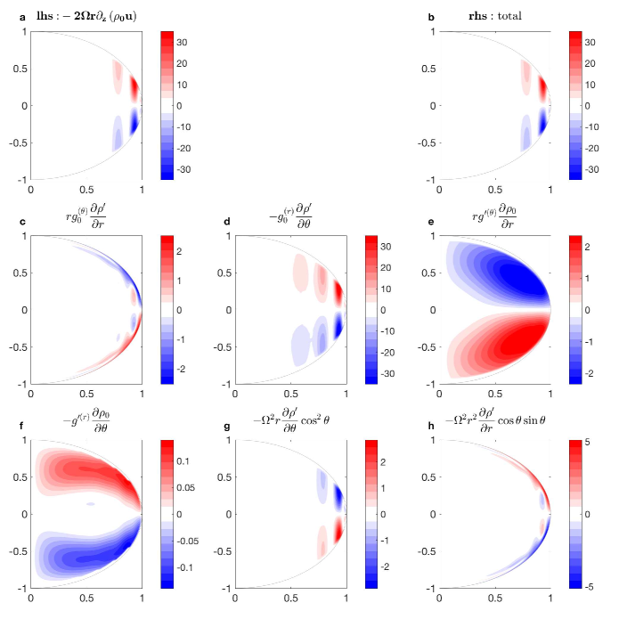
Figs. 5c,d show the solution to the null space part of the density, $\delta\rho^{\prime}$. It is negative everywhere, in order to compensate for $\hat{\rho}^{\prime}$ which is generally positive so that mass is conserved (section 2.3). The null space solution $\delta\rho^{\prime}$ is smaller than the full solution (Fig. 5a) by an order of magnitude. Furthermore, the latitude-dependent part of $\delta\rho^{\prime}$ (Fig 5d), which is the only part contributing to the gravity moments, is an order of magnitude smaller than $\delta\rho^{\prime}$ itself (Fig 5a). This explains why the contribution of $\delta\rho^{\prime}$ to the gravitational moments (Fig. 3, dashed line) is at least two orders of magnitude smaller than that of the non null-space part of the solution. Overall, this analysis shows that this perturbation approach gives, to leading order, results that are very close to those of the CMS.

Figure 5: Upper panels: the solution for $\rho^{\prime}$ (a) and the latitudinal depended part of the solution (b). Lower panels: the solution for $\delta\hat{\rho}^{\prime}$ (c) and its latitudinal dependent part (d). Unlike the eigenvectors (Fig. 2), the solution for the null space is large scale in both radius and latitude. It is negative everywhere (as a result of the need to compensate for $\delta\hat{\rho}^{\prime}$, which is positive everywhere). A large scale latitude depended structure exists, with the highest values close to the planet surface. All values are in kg m^-3.

3.2 Analysis of solution and comparison to previous approximations

We now assess the contribution of each term on the $rhs$ of the equation to the density solution (Fig. 4), and to the gravitational moments in particular. Since the equation is linear with respect to $\rho^{\prime}$ the analysis can be done by solving the equation when different terms are excluded. Following is a discussion of the thermal wind approximation of (Kaspi et al.,, 2010), and of the thermal-gravity wind solution of Zhang et al., (2015).

3.2.1 Spherically symmetric thermal wind approximation

The simplest solution to Eq. (6), the thermal wind (TW) approximation, is obtained when assuming that the static solution is spherically symmetric (Kaspi et al.,, 2010), density and gravity as in Figs. 1a,c) satisfying $\rho_{0}=\rho_{0}^{m}$, $g_{0}^{(r)}=g_{0}^{(r)m}$, and $g_{0}^{(\theta)}=0$, and neglecting the gravity anomaly ${\bf g}^{\prime}$, so that

$$\rho = \rho_{0}(r)+\rho^{\prime}(r,\theta),$$

$${\bf g} = g_{0}^{(r)}(r).$$ (19)

These assumptions reduce Eq. (6) to,

$$2\Omega r\partial_{z}\left(\rho_{0}u\right) = g_{0}^{(r)}\frac{\partial\rho^{\prime}}{\partial\theta},$$ (20)

where the centrifugal terms drop under the background sphericity assumptions (see discussion in section 4). The solution for the anomalous density can be simply found by integrating the rhs of Eq. (20) so that,

$$\rho^{\prime}(r,\theta) = \int^{\theta}\frac{2\Omega r}{g_{0}^{(r)}(r)}\partial_{z}\left(\rho_{0}(r)u(r,\theta^{\prime})\right)d\theta^{\prime}+\tilde{\rho}^{\prime}(r),$$ (21)

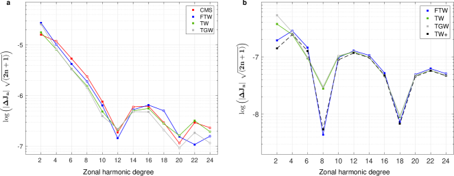
where $\tilde{\rho}^{\prime}$ is an unknown integration coefficient that does not contribute to the gravitational moments (see Eq. 18). Note that Eq. (20) is not the standard form of the thermal wind equation, e.g. Vallis, (2006), since it includes $\rho_{0}$ on the lhs, and the rhs is not a purely baroclinic term; nonetheless the two forms are equivalent (see details in Kaspi et al.,, 2016). Solving Eq. (21) and calculating the gravity moments using Eq. (17) we can compare the solution to the CMS method (Fig. 6a). The thermal wind solution follows the full CMS solution with the ratio between the calculated moments being $0.91,1.44,1.6,1.53,1.56,0.88$ for $J_{2},J_{4},...,J_{12}$, respectively. Note that in order to maintain the same framework, the equation was solved numerically using the same methodology as in the full case. Solving the equation using the method of Kaspi et al., (2010), which is much more efficient numerically, gives the same results up to numerical roundoff.

A variation on this case (Cao and Stevenson,, 2015), is to allow the background density $\rho_{0}$, as well as the gravity in the radial direction, $g_{0}^{(r)}$, to vary with latitude (Fig. 1b,d). The gravity in the latitudinal direction is kept zero. The resulting equation is the same as Eq. (21), but with the background fields being a function of both radius and latitude,

$$\rho^{\prime}(r,\theta) = \int^{\theta}\frac{2\Omega r}{g_{0}^{(r)}(r,\theta)}\partial_{z}\left(\rho_{0}(r,\theta)u(r,\theta^{\prime})\right)d\theta^{\prime}+\tilde{\rho}^{\prime}(r).$$ (22)

The solution to this approximation is very similar to the above simplified thermal wind balance (indistinguishable from the green line in Fig. 6), aside from some differences in the higher gravity moments, especially $J_{12}$ as was also found by Cao and Stevenson, (2015).

3.2.2 The thermal-gravity wind approximation

Next, we examine the contribution of the anomalous gravity to the solution, termed by Zhang et al., (2015) the thermal-gravity equation (TGW). They suggested that since the density perturbations $\rho^{\prime}$ result also in perturbations to the gravity field $\mathbf{g}\mathbf{{}^{\prime}}$, these in turn affect the solution, and therefore need to be included in the balance. As in Zhang et al., (2015) we assume the background state to vary with radius only, so that,

$$\rho = \rho_{0}(r)+\rho^{\prime}(r,\theta),$$ (23)

$${\bf g} = g_{0}^{(r)}(r)+\mathbf{g^{\prime}}(r,\theta).$$ (24)

These assumptions reduce Eq. (6) to,

$$-2\Omega r\partial_{z}\left(\rho_{0}u\right) = -g_{0}^{(r)}\frac{\partial\rho^{\prime}}{\partial\theta}+r\frac{\partial\rho_{0}}{\partial r}g^{\prime}{}^{(\theta)}.$$ (25)

This equation cannot be easily integrated in $\theta$, and needs to be solved numerically (Zhang et al.,, 2015). The resulting gravity moments are shown in Fig. 6a (gray), together with the thermal wind solution and the full perturbation method solution. The overall effect of the term added in Eq. (25) relative to the simplified thermal wind is small. It is mostly apparent in $J_{2}$ which increases by $54\%$. The effect on higher moments, not calculated in Zhang et al., (2015), is much smaller. The small effect of the additional term in TGW approximation is already clear from the magnitude of the relevant term Fig. 4e (repeating Fig. 4 with a radially dependent background state gives a similar structure and magnitude to that shown in Fig. 4a,c,e). Note that solving the equation with background fields that are both radially and latitudinally dependent shows similar results in the gravity moments.

Figure 6: The wind induced gravitational moments from several limits of Eq. 17. (a) For barotropic winds, showing the full solution (blue), standard thermal wind (green), and the thermal-gravity (gray). The CMS solution is shown in red for comparison. All solutions are quite similar, indicating that the simple TW approximation produces essentially the correct solution shown by the fuller approximations. (b) For a baroclinic case (with a wind-decay scale of 1000km). Shown are full solution (blue), standard thermal wind (green), and the thermal-gravity (gray) and a solution where the terms depending on $\partial\rho_{1}/\partial r$ are included (see text for discussion of the TW+ case).

3.3 The perturbation method in the more general case of baroclinic winds

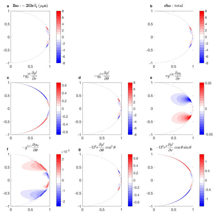
So far we have focused only on barotropic cases since the CMS solution, which we used as our reference, may only be obtained for barotropic winds. The FTW can be used also to analyze baroclinic winds, which are considered in this section. Using the baroclinic winds described in section 2.4 (decay depth of wind is 1000km), we repeat the above calculations of the density field and gravity moments. The gravitational moments for this case are shown in Fig. 4b, and the individual terms in the FTW equation are shown in Fig. 7.

The solution for the gravitational moments shows that the TW (Kaspi et al.,, 2010) and TGW (Zhang et al.,, 2015) solutions are again remarkably similar, apart from $J_{2}$. The solutions for both of these approximations are similar to the fuller FTW approximation, except for the moments $J_{2}$, $J_{6}$ and $J_{8}$. In particular, the fuller solution for $J_{8}$ is an order of magnitude smaller than both cruder approximations, underlining the importance of considering the additional physical effects included in this paper. In this case, there is a significant difference between TW (green) and the similar TGW (gray) on the one hand, and FTW (blue) on the other. The main reason for this difference are the two terms involving $\partial\rho^{\prime}/\partial r$. This is shown by the dash black curve denoted TW+, where we have used the TW solution plus the terms shown in panels c and h in Fig. 7, which both involve the radial derivative of the perturbation density. The importance of these terms is a direct consequence of the structure of the perturbation density solution, which tends to be strongly concentrated near the upper surface. This surface enhancement is not surprising given that the wind forcing decays rapidly away from the surface in this baroclinic case. This also implies that all terms in the equation tend to be more concentrated near the surface than in the barotropic case (compare Fig. 4 and Fig. 7). For this baroclinic case, the TGW term (panel e) is negligible relative to most other terms considered here. Note also, that the solution of the null space (section 2.3) relies on the barotropically based polyrtopic equation, therefore some inconsistencies might arise due to that. This, however, should not affect much the solutions since the null space contribution to the solution is small.

4 Discussion and conclusion

In the traditional approximation for terrestrial planets the centrifugal term is often merged with gravity in the momentum equation, by choosing the vertical direction to be that perpendicular to the planet’s geopotential surface and defining an effective gravity. This is then traditionally followed by approximating the planet as a sphere, so that the vertical direction coincides with the radial direction, and thus effectively neglecting the horizontal component of the centrifugal term. It is important to note that this centrifugal term is not smaller than the Coriolis term even for the Earth case, but because of the nearly spherical shape of Earth, this approximation allows trading a large dynamical component in the momentum balance with a small geometric error (Vallis,, 2006, section 2.2). This approximation has proven to hold well for Earth and other terrestrial planets. On the giant planets, the oblateness is not small (6.5% and 9.8% on Jupiter and Saturn, respectively, compared to 0.3% on Earth). Therefore, the contribution of the centrifugal (fifth and sixth terms on the rhs of Eq. 6) and self-gravitation terms (third and fourth terms on the rhs of Eq. 6) can potentially lead to significant contributions to the momentum balance, and therefore may alter thermal-wind balance as well. The goal of this study is to assess the importance of these terms in a fluid planet.

By solving numerically the full second order momentum equation in our perturbation approach, which includes the original thermal-wind balance terms (lhs term and second term on rhs in Eq. 6), self-gravity terms, centrifugal terms, and other non-spherical contributions (first term on rhs of Eq. 6), we have shown that the original thermal wind balance is still the leading order. In the barotropic limit, the thermal wind results, with the various higher order contributions, are systematically compared to results from the oblate concentric Maclaurin spheroids (CMS) model. In the context of recent studies that argue that additional terms are important in the balance for calculating the gravitational moments (Zhang et al.,, 2015; Cao and Stevenson,, 2015), we show that to leading order these terms are negligible, and have a small contribution to the gravity moments. Consistently with Zhang et al., (2015), we find that the self-gravity term (TGW) increases the value of $J_{2}$, though it does not bring the thermal wind $J_{2}$ closer to the CMS result. This terms has a negligible contribution to all higher harmonics, which were not discussed in Zhang et al., (2015).

Figure 7: Solution of Eq. 6 for a baroclinic case (depth of winds is 1000 km) when all terms are included. (a) $lhs$ term, (b) total $rhs$, (c-h) the six terms on the $rhs$. Values of $\rho$’ are in kg m^-3.

We conclude therefore that while more complete solutions are possible, as we do in this study, the traditional thermal-wind gives a very good approximation to the balance between the wind shear and the density gradients, and integrating it gives a very good approximation to the gravity moments. Particularly, taking into account the accuracy of the Juno and Cassini measurements, this gives an excellent approximation. Quantitatively, for the barotropic cases, its results differ by at most a factor of 1.6 compared to the full solution. This difference is small considering the other uncertainties of the interior flow. For the baroclinic case, where wind structures decay rapidly near the surface, terms involving the radial derivative of the perturbation density become more important for calculating the gravity moments.

The main advantage of using the thermal wind (TW) model compared to full, self-consistent thermal wind (FTW) is numerical. While the TW equation (21) allows for local calculation of the density from the wind, the FTW equation (6) is an integro-differential equation that needs to be solved globally. It is mostly complicated from the need to integrate the dynamical density ($\rho^{\prime}$ ) globally to calculate the dynamical self-gravity ($\mathbf{g^{\prime}}$). The TW approximation allows therefore using much higher resolution, which is necessary for resolving the high order moments. As a consequence of the simplicity of the TW model, more sophisticated and numerically demanding methods can be applied in order to find the best matching wind field given the gravity measurements (Galanti and Kaspi, 2016a, ; Galanti and Kaspi, 2016b, ). The inevitability of the solution using the TW model is a major advantage for the upcoming analysis of the Juno and Cassini data. Given the extremely small contribution of the null space to the overall solution, we expect that the more complete FTW model would also be invertible, still the computational challenge involved is much greater.

In summary, deciphering the effect of the atmospheric and internal flows from the measured gravity spectrum of Jupiter and Saturn provides a major challenge. The methods suggested to date have been either limited to barotropic cases (e.g., Hubbard,, 1982, 1999, 2012; Kong et al.,, 2012; Hubbard et al.,, 2014), or approximations limited to spherical symmetry or partial solutions (e.g., Kaspi et al.,, 2010; Zhang et al.,, 2015; Cao and Stevenson,, 2015). Here, we have developed a self-consistent perturbation approach to the thermal wind balance that incorporates all physical effects, including the effects of oblateness on the dynamics and the gravity perturbation induced by the flow itself. The full self-consistent perturbation approach to the thermal wind balance considered here allows to objectively examine the role of different physical processes, allows obtaining and even more accurate approximation by proceeding to higher order perturbation corrections (Appendix A.2), and allows interpreting the expected Juno and Cassini observations in a more complete way than was possible in previous approaches, thus maximizing the benefits of these observations.

Acknowledgements: We thank the Juno science team interiors working group for valuable discussions. ET is funded by the NSF Physical Oceanography program, grant OCE-1535800, and thanks the Weizmann Institute of Science (WIS) for its hospitality during parts of this work. YK and EG acknowledge support from the Israeli Ministry of Science (grant 45-851-641), the Minerva foundation with funding from the Federal German Ministry of Education and Research, and from the WIS Helen Kimmel Center for Planetary Science.

Appendix A Appendices

A.1 Higher order perturbation equations

We write here the perturbation equations to the second order to demonstrate how the results of our approach can be made more accurate if needed. The momentum equation (2) is,

$$2\boldsymbol{\Omega}\mathbf{\times}\left(\rho\mathbf{u}\right) = -\nabla p-\rho{\bf g}-\rho\boldsymbol{\Omega}\times\boldsymbol{\Omega}\mathbf{\times r}.$$ (26)

Writing the density as $\rho=\rho_{0}+\rho_{1}+\rho_{2}$, and substituting into the above equation, treating $\rho_{1}$ as an order $\epsilon$ correction and $\rho_{2}$ as an order $\epsilon^{2}$ correction, we can separate the different orders to find equations for each correction order. Note that in the previous sectinos we denote $\rho_{1}$ as $\rho^{\prime}$. We view, as defined earlier, the zeroth order balance as the balance without the effects of the winds, so that our zeroth order equation is,

$$0 = -\nabla p_{0}-\rho_{o}g_{0}-\rho_{0}\boldsymbol{\Omega}\times\boldsymbol{\Omega}\mathbf{\times r}.$$ (27)

The winds enter at the first order, where the equation is

$$2\boldsymbol{\Omega}\mathbf{\times}\left(\rho_{0}\mathbf{u}\right) = -\nabla p_{1}-\rho_{o}{\bf g}_{1}-\rho_{1}{\bf g}_{0}-\rho_{1}\boldsymbol{\Omega}\times\boldsymbol{\Omega}\mathbf{\times r},$$ (28)

and the second order correction is then obtained by solving

$$2\boldsymbol{\Omega}\mathbf{\times}\left(\rho_{1}{\bf u}\right) +\text{$\rho_{1}{\bf g}_{1}$}= -\nabla p_{2}-\rho_{o}{\bf g}_{2}-\rho_{2}{\bf g}_{0}-\rho_{2}\boldsymbol{\Omega}\times\boldsymbol{\Omega}\mathbf{\times r}.$$ (29)

In the second order perturbation equation we moved all terms that are known from previous orders to the lhs. This equation is again solved by taking a curl and then taking care of the integration constant (null space solution) if needed. Because the second order equation is generally similar to the first order equation, its numerical solution follows the same approach and should not pose significant additional difficulties. While this procedure should be formally done in a non-dimensional form, we present here the dimensional equations for clarity. The small parameter in this expansion when it is done in non-dimensional form is the Rossby number $Ro=(\Omega U)/L$, where $U$ is a scale for the velocity and $L$ the horizontal length scale of the relevant motions.

A.2 Integration constant and null space

The objective of this appendix is to show how the integration constant encountered in the thermal wind approach (e.g., Kaspi et al.,, 2010; Zhang et al.,, 2015) can be calculated. This is meant to aid the understanding of our approach to solving for the null space of the more general solution considered in the main text. The main message of this appendix is that the integration constant may be determined by adding the missing physics of the polytropic equation, and by requiring the total mass of the density perturbation to vanish. The momentum equation for the simple example is,

$$0=-\nabla p-\mathbf{g}\rho+\Omega^{2}\rho r\cos\theta\hat{r}_{\perp}.$$ (30)

We treat the effects of rotation as a perturbation and the leading order balance is then hydrostatic, with the corresponding fields being a function of radius alone ($\rho_{0}=\rho_{0}\left(r\right)$),

$$0=-\nabla p_{0}-\mathbf{g}_{0}\rho_{0}.$$ (31)

The next order contains the deviations in density and gravity due to rotation,

$$0=-\nabla p_{1}-\mathbf{g}_{1}\rho_{0}-\mathbf{g}_{0}\rho_{1}+\Omega^{2}\rho_{0}r\cos\theta\hat{r}_{\perp}.$$ (32)

Taking the curl,

$$0 = -g_{1}^{(\theta)}r\frac{\partial\rho_{0}}{\partial r}+g_{0}\frac{\partial\rho_{1}}{\partial\theta}-\Omega^{2}r^{2}\frac{\partial\rho_{0}}{\partial r}\cos\theta\sin\theta,$$ (33)

substituting the expression for the gravity fields, and integrating over $\theta$,

$$-\frac{1}{2}\Omega^{2}r^{2}\frac{\partial\rho_{0}}{\partial r}\cos^{2}\theta = g_{0}\rho_{1}+2\pi G\frac{\partial\rho_{0}}{\partial r}\iint\frac{\mathbf{\rho_{{}_{1}}}(r^{\prime},\theta^{\prime})r\mathbf{{}^{\prime 2}}\sin(\theta^{\prime})}{\langle|\mathbf{r-}\mathbf{r}^{\prime}|\rangle}dr^{\prime}d\theta^{\prime}+C(r),$$ (34)

where $C(r)$ is the unknown integration constant to be solved for, and the lhs is a known forcing term due to rotation by to the already known zeroth order solution. The perturbation density can be expressed as the sum of $\hat{\rho}_{1}(r,\theta)$ that solves the above equation with the integration constant set to zero, and $\delta\rho_{1}(r)$ that satisfies the same equation with a zero on the lhs and with the integration constant. Together, $\rho_{1}=\hat{\rho}_{1}(r,\theta)+\delta\rho_{1}(r)$ solves Eq. 34.

Given that we took the curl of the momentum equation, $\hat{\rho}_{1}$ which solves the above equation without $C(r)$ satisfies the original momentum equation up to a gradient of some function which we may write as $\hat{p}_{1}+\delta p_{1}$,

$$0=-\nabla(p_{1}+\delta p_{1})+\rho_{0}\mathbf{\hat{g}}_{1}+\hat{\rho}_{1}\mathbf{g}_{0}+\rho_{0}\Omega^{2}r\cos\theta\hat{r}_{\perp}.$$

Next, take the difference between the momentum equation for $\rho_{1}$ and for $\hat{\rho}_{1}$, we find,

$$0=-\nabla\delta p_{1}+\rho_{0}\mathbf{\delta g}_{1}+\delta\rho_{1}\mathbf{g}_{0}.$$ (35)

The second and third terms in 35 are functions of radius $r$ only. Therefore we expect the pressure term $-\nabla\delta p_{1}$ to also be a function of the radius only. Furthermore, assuming now that the polytropic relation holds for the perturbation pressure and density, we have

$$\delta p_{1}=Kn\rho_{0}\delta\rho_{1}$$

which leads to an equation for the unknown perturbation density,

$$0=-\nabla\left(Kn\rho_{0}\delta\rho_{1}\right)+\rho_{0}\mathbf{\delta g}_{1}+\delta\rho_{1}\mathbf{g}_{0}.$$

Substituting the expression for the gravity,

$$0 = -\frac{\partial}{\partial r}\left(Kn\rho_{0}\delta\rho_{1}\right)+\rho_{0}2\pi G\frac{\partial}{\partial r}\iint\left\langle\frac{1}{|\mathbf{r-}\mathbf{r}^{\prime}|}\right\rangle\delta\rho_{1}(r^{\prime})r\mathbf{{}^{\prime 2}}\sin(\theta^{\prime})dr^{\prime}d\theta^{\prime}+\delta\rho_{1}\mathbf{g}_{0},$$ (36)

and substituting the zeroth order solutions for $\rho_{0},$ $p_{0}$ and $g_{0}$ (Zhang et al., (2015), see notation there), and after some more rearrangement and integration in $\xi$ we get,

$$0 = -\delta\rho_{1}+\frac{1}{2}\iint\left\langle\frac{1}{|\mathbf{\xi-}\xi^{\prime}|}\right\rangle\delta\mathbf{\rho_{{}_{1}}}(\xi^{\prime})\xi\mathbf{{}^{\prime 2}}\sin(\theta)d\xi^{\prime}d\theta+D$$ (37)

where $D$ is the constant of integration. Use the expansion for the average over longitude (Zhang et al.,, 2015), and the fact that the integral over all Legendre polynomials but the first vanish,

$$0 = -\delta\rho_{1}(\xi)+\int_{0}^{\pi}f_{0}(\xi,\xi^{\prime})\delta\mathbf{\rho_{{}_{1}}}(\xi^{\prime})\xi\mathbf{{}^{\prime 2}}d\xi^{\prime}+D,$$ (38)

where,

$$f_{0}(\xi,\xi^{\prime})=\begin{cases}\frac{1}{\xi}&\xi^{\prime}\leq\xi\\ \frac{1}{\xi^{\prime}}&\xi^{\prime}>\xi\end{cases}.$$

A solution may be found by assuming a Frobenius-form solution,

$$\delta\rho_{1}(\xi)=\sum_{m=0}^{\infty}a_{m}\xi{}^{m+r}.$$

Now find what is $a_{m}.$ Write Eq. (38) explicitly

$$0 = -\sum_{m=0}^{\infty}a_{m}\xi^{m+r}+\sum_{m=0}^{\infty}\int_{0}^{\xi}\frac{1}{\xi}a_{m}\xi^{\prime m+r}\xi\mathbf{{}^{\prime 2}}d\xi^{\prime}+\sum_{m=0}^{\infty}\int_{\xi}^{\pi}\frac{1}{\xi^{\prime}}a_{m}\xi^{\prime m+r}\xi\mathbf{{}^{\prime 2}}d\xi^{\prime}+D,$$ (39)

and performing the integral and collecting powers, while also defining $a_{-1}=a_{-2}=0$ ,

$$0 =\sum_{m=0}^{\infty}\left(-a_{m}+\frac{1}{\left(m+1+r\right)}a_{m-2}-\frac{1}{m+r}a_{m-2}\right)\xi^{m+r}+\sum_{m=0}^{\infty}\frac{1}{m+2+r}a_{m}\pi^{m+2+r}+D.$$ (40)

The coefficient of $\xi^{m+r}$ should vanish for all $m$, giving us the recursion relation. Multiplying by $(m+r)(m+r+1)$ and considering the $m=0$ and $m=1$ cases, and we find that there are two possible solutions for the Frobenius power, $r=0$ or $r=-1$. The first leads to the recursion relation,

$$a_{m} = -\frac{1}{m(m+1)}a_{m-2}.$$

We term this solution $F_{1}(\xi).$ The second solution, with $r=-1$, leads to

$$a_{m} = -\frac{1}{(m-1)m}a_{m-2},$$ (41)

which is the recursion relation for cosine. Therefore,

$$\delta\rho_{1}=C_{1}F_{1}+C_{2}\frac{\cos(\xi)}{\xi}.$$

The $\cos(\xi)/\xi$ solution is not physical because it diverges at $\xi=0$ and we conclude that $C_{2}=0$. Considering the coefficients of $\xi^{0}$ in Eq. 40 we find $a_{0}$ in terms of the unknown integration constant $D$. We may then use $D$ to satisfy the constraint that volume integral over the total perturbation $\rho_{1}(\xi,\theta)+\delta\rho_{1}(\xi)$ should vanish, as done in the manuscript for the fuller problem considered there.

References

- Busse, (1976) Busse, F. H. (1976). A simple model of convection in the Jovian atmosphere. Icarus, 29:255–260.
- Cao and Stevenson, (2015) Cao, H. and Stevenson, D. J. (2015). Gravity and zonal flows of giant planets: From the euler equation to the thermal wind equation. ArXiv e-prints.
- Cho and Polvani, (1996) Cho, J. and Polvani, L. M. (1996). The formation of jets and vortices from freely-evolving shallow water turbulence on the surface of a sphere. Phys. of Fluids., 8:1531–1552.
- (4) Galanti, E. and Kaspi, Y. (2016a). An adjoint based method for the inversion of the Juno and Cassini gravity measurements into wind fields. Astrophys. J., 820:91.
- (5) Galanti, E. and Kaspi, Y. (2016b). Deciphering Jupiters deep flow dynamics using the upcoming Juno gravity measurements and an adjoint based dynamical model. Icarus. submitted.
- Guillot, (2005) Guillot, T. (2005). The interiors of giant planets: Models and outstanding questions. Ann. Rev. Earth Plan. Sci., 33:493–530.
- Heimpel et al., (2016) Heimpel, M., Gastine, T., and Wicht, J. (2016). Simulation of deep-seated zonal jets and shallow vortices in gas giant atmospheres. Nature Geoscience, 9:19–23.
- Helled and Guillot, (2013) Helled, R. and Guillot, T. (2013). Interior models of saturn: Including the uncertainties in shape and rotation. Astrophys. J., 767:113.
- Hubbard, (1982) Hubbard, W. B. (1982). Effects of differential rotation on the gravitational figures of Jupiter and Saturn. Icarus, 52:509–515.
- Hubbard, (1999) Hubbard, W. B. (1999). Note: Gravitational signature of Jupiter’s deep zonal flows. Icarus, 137:357–359.
- Hubbard, (2012) Hubbard, W. B. (2012). High-precision Maclaurin-based models of rotating liquid planets. Astrophys. J. Let., 756:L15.
- Hubbard, (2013) Hubbard, W. B. (2013). Conventric maclaurian spheroid models of rotating liquid planets. Astrophys. J., 768(1).
- Hubbard et al., (2014) Hubbard, W. B., Schubert, G., Kong, D., and Zhang, K. (2014). On the convergence of the theory of figures. Icarus, 242:138–141.
- Ingersoll and Pollard, (1982) Ingersoll, A. P. and Pollard, D. (1982). Motion in the interiors and atmospheres of Jupiter and Saturn: Scale analysis, anelastic equations, barotropic stability criterion. Icarus, 52:62–80.
- Kaspi, (2013) Kaspi, Y. (2013). Inferring the depth of the zonal jets on Jupiter and Saturn from odd gravity harmonics. Geophys. Res. Lett., 40:676–680.
- Kaspi et al., (2016) Kaspi, Y., Davighi, J. E., Galanti, E., and Hubbard, W. B. (2016). The gravitational signature of internal flows in giant planets: comparing the thermal wind approach with barotropic potential-surface methods. Icarus, 276:170–181.
- Kaspi and Flierl, (2007) Kaspi, Y. and Flierl, G. R. (2007). Formation of jets by baroclinic instability on gas planet atmospheres. J. Atmos. Sci., 64:3177–3194.
- Kaspi et al., (2010) Kaspi, Y., Hubbard, W. B., Showman, A. P., and Flierl, G. R. (2010). Gravitational signature of Jupiter’s internal dynamics. Geophys. Res. Lett., 37:L01204.
- Kaspi et al., (2013) Kaspi, Y., Showman, A. P., Hubbard, W. B., Aharonson, O., and Helled, R. (2013). Atmospheric confinement of jet-streams on Uranus and Neptune. Nature, 497:344–347.
- Kong et al., (2012) Kong, D., Zhang, K., and Schubert, G. (2012). On the variation of zonal gravity coefficients of a giant planet caused by its deep zonal flows. Astrophys. J., 748.
- Lian and Showman, (2010) Lian, Y. and Showman, A. P. (2010). Generation of equatorial jets by large-scale latent heating on the giant planets. Icarus, 207:373–393.
- Liu and Schneider, (2010) Liu, J. and Schneider, T. (2010). Mechanisms of jet formation on the giant planets. J. Atmos. Sci., 67:3652–3672.
- Liu et al., (2014) Liu, J., Schneider, T., and Fletcher, L. N. (2014). Constraining the depth of saturn’s zonal winds by measuring thermal and gravitational signals. Icarus, 239:260–272.
- Liu et al., (2013) Liu, J., Schneider, T., and Kaspi, Y. (2013). Predictions of thermal and gravitational signals of Jupiter’s deep zonal winds. Icarus, 224:114–125.
- Militzer et al., (2008) Militzer, B., Hubbard, W. B., Vorberger, J., Tamblyn, I., and Bonev, S. A. (2008). A massive core in Jupiter predicted from first-principles simulations. Astrophys. J., 688:L45–L48.
- Nettelmann et al., (2012) Nettelmann, N., Becker, A., Holst, B., and Redmer, R. (2012). Jupiter models with improved Ab initio hydrogen equation of state (H-REOS.2). Astrophys. J., 750:52.
- Porco et al., (2003) Porco, C. C., West, R. A., McEwen, A., Del Genio, A. D., Ingersoll, A. P., Thomas, P., Squyres, S., Dones, L., Murray, C. D., Johnson, T. V., Burns, J. A., Brahic, A., Neukum, G., Veverka, J., Barbara, J. M., Denk, T., Evans, M., Ferrier, J. J., Geissler, P., Helfenstein, P., Roatsch, T., Throop, H., Tiscareno, M., and Vasavada, A. R. (2003). Cassini imaging of Jupiter’s atmosphere, satellites and rings. Science, 299:1541–1547.
- Scott and Polvani, (2007) Scott, R. K. and Polvani, L. M. (2007). Forced-dissipative shallow-water turbulence on the sphere and the atmospheric circulation of the giant planets. J. Atmos. Sci., 64:3158–3176.
- Showman et al., (2006) Showman, A. P., Gierasch, P. J., and Lian, Y. (2006). Deep zonal winds can result from shallow driving in a giant-planet atmosphere. Icarus, 182:513–526.
- Showman et al., (2016) Showman, A. P., Kaspi, Y., Achterberg, R., and Ingersoll, A. P. (2016). Saturn in the 21st Century, chapter The global atmospheric circulation of Saturn. Cambridge University Press.
- Strang, (2006) Strang, G. (2006). Linear algebra and its applications. 4th ed. Belmont, CA: Thomson, Brooks/Cole.
- Vallis, (2006) Vallis, G. K. (2006). Atmospheric and Oceanic Fluid Dynamics. pp. 770. Cambridge University Press.
- Vasavada and Showman, (2005) Vasavada, A. R. and Showman, A. P. (2005). Jovian atmospheric dynamics: An update after Galileo and Cassini. Reports of Progress in Physics, 68:1935–1996.
- Williams, (1978) Williams, G. P. (1978). Planetary circulations: 1. barotropic representation of the Jovian and terrestrial turbulence. J. Atmos. Sci., 35:1399–1426.
- Wisdom and Hubbard, (2016) Wisdom, J. and Hubbard, W. B. (2016). Differential rotation in Jupiter: A comparison of methods. Icarus, 267:315–322.
- Zhang et al., (2015) Zhang, K., Kong, D., and Schubert, G. (2015). Thermal-gravitational wind equation for the wind-induced gravitational signature of giant gaseous planets: Mathematical derivation, numerical method and illustrative solutions. Astrophys. J., 806:270–279.