High-dimensional entanglement certification

Abstract

Quantum entanglement is the ability of joint quantum systems to possess global properties (correlation among systems) even when subsystems have no definite individual property. Whilst the 2-dimensional (qubit) case is well-understood, currently, tools to characterise entanglement in high dimensions are limited. We experimentally demonstrate a new procedure for entanglement certification that is suitable for large systems, based entirely on information-theoretics. It scales more efficiently than Bell’s inequality, and entanglement witness. The method we developed works for arbitrarily large system dimension $d$ and employs only two local measurements of complementary properties. This procedure can also certify whether the system is maximally entangled. We illustrate the protocol for families of bipartite states of qudits with dimension up to $32$ composed of polarisation-entangled photon pairs.

Introduction

As the dimension of investigated systems increases, it becomes more complicated to demonstrate their quantum effects arndt2014testing ; sciarrino2013quantum ; friedman2000quantum . Indeed, a full characterization (quantum tomography) becomes practically impossible already for systems of rather small dimensionality PhysRevA.66.062305 ; artiles2005invitation . It is therefore important to explore new avenues to prove the presence of such effects, e.g. entanglement, for arbitrary dimensions. High-dimensional entangled states offer a larger code space, attracting interests for quantum key distribution mair2001entanglement , teleportation PhysRevLett.69.2881 and security-enhanced quantum cryptography PhysRevLett.88.127901 ; PhysRevA.69.032313 .

In this context, proving that one has achieved entanglement (entanglement certification) and detecting entanglement are different primitives. Indeed, entanglement detection methods bruss2002characterizing ; RevModPhys.81.865 ; Ghne20091 must be as sensitive as possible and must be able to detect the largest possible class of entangled states. Often such methods are inapplicable to large system dimensions or scale poorly with increasing dimension as they entail increasingly complicated measurements and data analysis. Entanglement detection such as witness operators, for instance, typically requires a number of local measurement settings that scales linearly in $d$ guhne2003experimental . In contrast, entanglement certification refers to the fact that one has simply to prove that the system is entangled. To do entanglement certification, one can optimize the method to the specific entangled state that one is producing. It must fulfill different requirements: it must be as robust and simple as possible. In other words a good method for entanglement detection can also work for entanglement certification, but not vice versa.

Here we present an entanglement certification procedure that is extremely simple to implement (the measurement of two local observables PhysRevA.75.012336 ; PhysRevA.75.062317 suffices), is compatible with current state-of-the-art experimental techniques, and can be easily scaled up to arbitrary dimension. In addition to certifying the production of entangled states, our procedure can also certify the production of maximal entanglement. To prove its simplicity, we present an experimental test that uses entangled systems with dimension up to $d=32$, constructed by suitably grouping couples of entangled photon pairs. In the general case, for a two-qudit experiment with arbitrary $d$, two measures would still be sufficient to implement our method, but not sufficient for tomography or other entanglement detection methods. To certify the presence of entanglement, one has only to calculate the (classical) correlations among the measurement outcomes of the two observables, for example, through their mutual information. If such correlations are larger than some threshold, the state is guaranteed to be entangled (Fig. 1). If they attain their maximum value, the state must be maximally entangled.

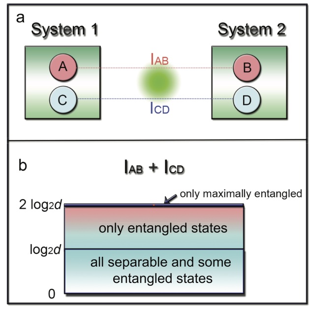
Figure 1: Illustration of the procedure. (a) Measure two complementary observables: $AB$ and $CD$, where $A,C$ are observables for system 1 and $C,D$ for system 2. Then calculate the mutual information $I_{AB}$ and $I_{CD}$ of their outcomes. (b) If the value of the sum $I_{AB}+I_{CD}$ is larger than log${}_{2}(d)$ bits ($d$ being the system dimension), then the two systems are certified to be entangled. If the value of the sum is 2log${}_{2}(d)$ bits, they are certified to be maximally entangled.

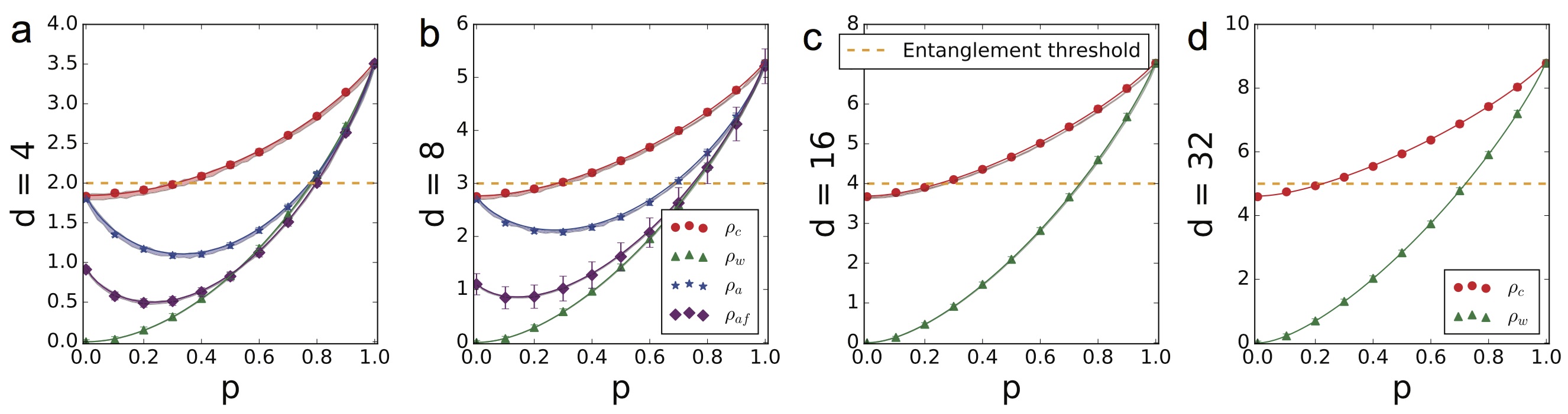
Figure 2: Experimental test of the method for $d$-dimensional systems. The plots refer to the experimentally determined sum of mutual information $I_{AB}+I_{CD}$ for $\rho_{c}$ of equation (6) (red circles), $\rho_{w}$ of equation (7) (green triangles), $\rho_{a}$ of equation (8) (blue stars when $CD$ is the $\sigma_{x}$ observable, and purple diamonds when $CD$ is the Fourier basis). The points that fall above the entanglement threshold (orange dashed line) refer to states that are certified to be entangled. Taking into account the confidence interval of the measurement outcome, the state was maximally entangled if the maximum sum $I_{AB}+I_{CD}=2\log_{2}d$ is achieved. The bands are a Monte Carlo simulation, taking into account realistic experimental conditions (eg. phase inaccuracy due to the wave plates used in state tuning); for $d=32$ they are narrower than the fit. The error bars represent bounds for 2 standard deviations (95$\%$ confidence), for most of the data points the error bars are smaller than the markers.

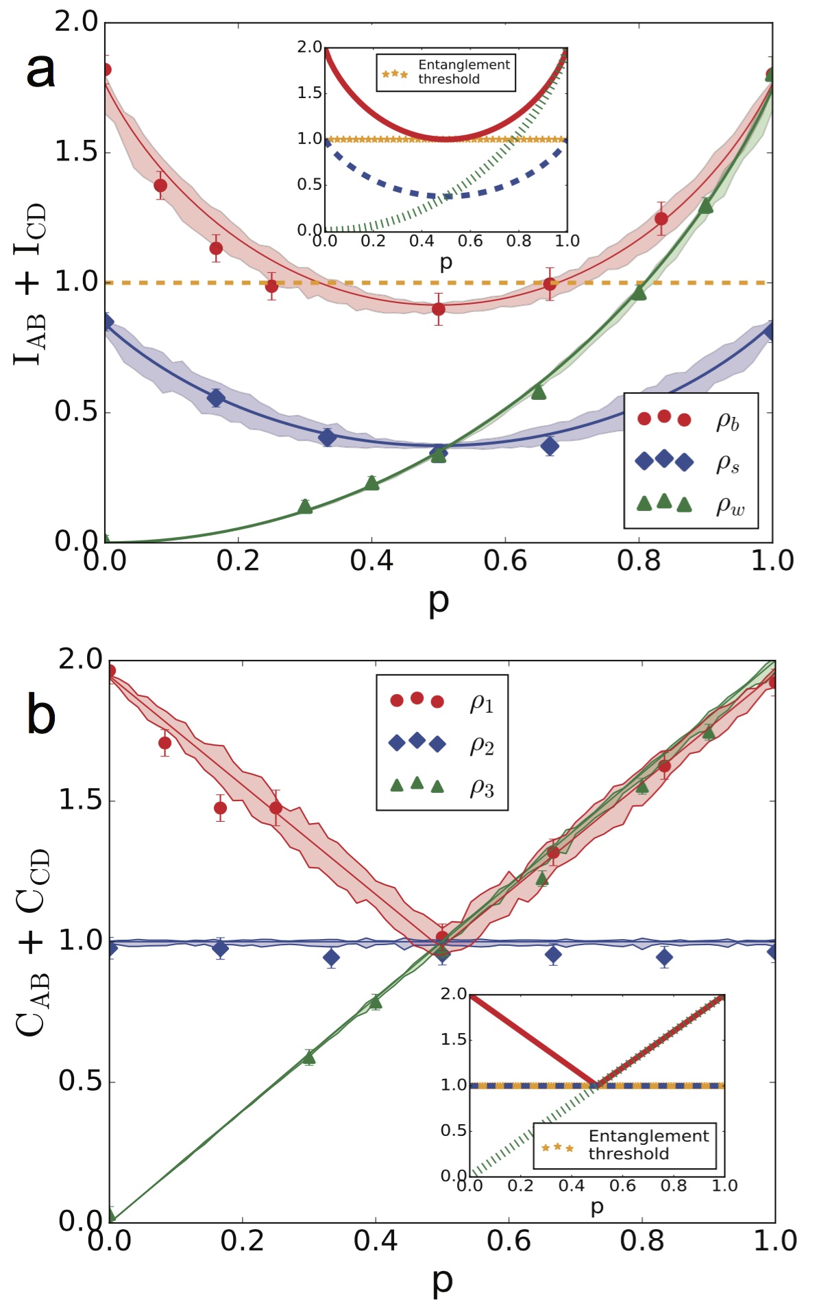
Figure 3: Experimental comparison between mutual information (above) and Pearson coefficient (below). The insets show the theoretical curves. The data points refer to $\rho_{b}$ of equation (10) (red circles), $\rho_{s}$ of equation (LABEL:eq:classical) (blue diamonds), $\rho_{w}$ of equation (7) (green triangles) for $d=2$. The states whose data points are strictly above the entanglement threshold ($I_{AB}+I_{CD}=1$ for the upper graph and $C_{AB}+C_{CD}=1$ for the lower graph, conjectured) are certified to be entangled. In the lower graph this threshold overlaps with the fit for $\rho_{s}$, which is then not entangled, as expected. The markers represent the data points, the lines represent a fit from reconstructed density matrices, and the bands are a Monte Carlo simulation, taking into account realistic experimental conditions (eg. phase inaccuracy due to the wave plates used in state tuning). The error bars represent bounds for 2 standard deviations. It is evident that the experimental results are in good agreement with the theoretical values.

If $A$ and $C$ are complementary properties, the knowledge of $A$ gives no information on $C$ and vice versa. This happens whenever $|\braket{a}{c}|^{2}=1/d$, for all $|a\rangle$ and $|c\rangle$ eigenstates of the observables $A$ and $C$, where $d$ is the Hilbert space dimension. This is equivalent to two sets of mutually unbiased bases (MUB’s). Consider the two-qubit maximally entangled state $|\Phi^{+}\rangle\propto|00\rangle+|11\rangle$; it clearly has maximal correlation among results for the observables with eigenstates $|0\rangle,|1\rangle$: both qubits have the same value. This state has also maximal correlation among results for a complementary observable with eigenvalues $|\pm\rangle=\frac{1}{\sqrt{2}}(|0\rangle\pm|1\rangle)$, since it can be written as $|\Phi^{+}\rangle\propto|++\rangle+|--\rangle$. Thus, the mutual information between measurement outcomes on the two qubits is one bit per observable, summing to two bits. If one has only separable states, the sum cannot be larger than one: for example, the classically correlated state $\rho\propto\ket{00}\bra{00}+\ket{11}\bra{11}$ has one bit of mutual information for the outcomes of the first observable, but zero bits for the outcomes of the second.

Starting from the theoretical suggestions of maccone2014complementarity , we extend the method from the qubit ($d=2$) case to arbitrary high dimensions. The proposed mechanism to certify entanglement thus uses the following procedure:

1. Identify two bipartite complementary observables $AB$ and $CD$, where $A,C$ are system 1 observables and $B,D$ are system 2 observables (Fig. 1a).

2. Measure the statistics of the outcomes of the two observables: local measurements on the two systems suffice.

3. These measurements return the joint probabilities $p(a_{o},b_{o})$ of obtaining outcome $a_{o}$ on system 1 for $A$ and $b_{o}$ on system 2 for $B$, and $p(c_{o},d_{o})$ of obtaining outcome $c_{o}$ on system 1 and $d_{o}$ on system 2. Use them to calculate the mutual information $I_{AB}$ among measurement results for $AB$ and $I_{CD}$ among results for $CD$, with

   $$I_{AB}\equiv\sum_{ab}p(a,b)\log_{2}\frac{p(a,b)}{\sum_{a}p(a,b)\sum_{b}p(a,b)}.$$ (1)

4. Certification: if $I_{AB}+I_{CD}>\log_{2}d$, the two systems are entangled; if $I_{AB}+I_{CD}=2\log_{2}d$, the two systems are maximally entangled.

The proof of these statements, based on Maassen and Uffink’s entropic uncertainty relation PhysRevLett.60.1103 is given in maccone2014complementarity (see also PhysRevA.90.062119 ; PhysRevA.89.022112 ; PhysRevLett.108.210405 ).

In regards to the choosing the observables, for pure states, the obvious choice would be the Schmidt bases and their respective Fourier bases. Whilst for mixed states, one can diagonalise the density matrix, identify the eigenvector with the largest weight and use the Schmidt basis (and its respective Fourier bases). Alternatively, one can choose the bases that diagonalises the reduced density matrices. While there is no guarantee that these choices will allow one to implement the procedure, they are the ones that may uncover the most correlations.

This method is simple to implement for systems of any dimensionality: it only entails independent measurements of two local observables on the two systems. Moreover, it is robust since, although one can optimize the choice of observables to maximize the sum of mutual information, the systems are guaranteed to be entangled if the above conditions are satisfied for any couple of complementary observables. It is interesting to note that, coherently performing sequential complementary measurements on the same system may generate the entanglement itself PhysRevA.89.010302 .

To date, the most prominent way of producing higher dimensional entangled systems is via the orbital angular momentum degree of freedom of a photon fickler2012quantum ; dada2011experimental ; mair2001entanglement ; schemes to produce three-level entangled states in trapped ions have also been proposed PhysRevA.68.035801 ; PhysRevA.77.014303 . Our method, however, works for any d-dimensional system as long as the appropriate measurements can be performed.

Based on the theoretical work by Collins et al., other recent experiments dada2011experimental ; lo2015experimental have studied higher dimensional entangled system via generalised Bell’s inequalities, where the correlations between the two measurement settings on each are studied. The violation of Bell’s inequality is usually discussed in terms of quantum non-locality. In this context, the framework of hidden variable theories is in general specified by the 4 measurement settings, each with $d$ outcomes, therefore needing $d^{4}$ joint probabilites collins2002bell to describe the system globally. In this case, collins2002bell ; dada2011experimental ; lo2015experimental examine two settings on each system, and how the observables on one system are correlated with the two observables on the second system, requiring a total of $2d\times 2d$ joint outcomes. On the other hand, our method is based on entropic relations, requiring only two measurement settings, and is completely specified by $2d^{2}$ probabilities. Similarly to lo2015experimental , we used ensembles of individual entangled photon pairs to construct a higher dimensional state. All the subsystems that compose this state do not exist at the same time, but that is irrelevant to our current aims.

To demonstrate the method in practice, we performed an experiment using high-dimensional entangled systems. We certify the presence of entanglement for various families of states, by measuring pairs of complementary observables. These families are obtained by appropriately grouping couples of polarisation entangled photonic qubits, mapping qudits onto qubits:

$$\frac{1}{\sqrt{d}}\sum_{j=0}^{d-1}\ket{j}\ket{j} = \frac{1}{\sqrt{d}}\Big{(}\ket{00}+\ket{11}\Big{)}^{\otimes n},$$ (2)

where this mapping is obtained by expressing $j$ in binary notation and rearranging the qubits in such a way that the ones placed in odd positions in the tensor products on the right hand side are assigned to system 1 while the ones in even positions to system 2. For example, a $d=4$ maximally entangled state can be expressed as $(\ket{00}+\ket{11}+\ket{22}+\ket{33})/2\equiv(\ket{00\,00}+\ket{01\,01}+\ket{10\,10}+\ket{11\,11})/2\equiv(\ket{0}_{\alpha}\ket{0}_{\beta}+\ket{1}_{\alpha}\ket{1}_{\beta})\otimes(\ket{0}_{\gamma}\ket{0}_{\delta}+\ket{1}_{\gamma}\ket{1}_{\delta})/2,$ where qubits labeled $\alpha$ and $\gamma$ belong to system 1, while $\beta$ and $\delta$ to system 2. It would also be extremely interesting to show that one could coherently manipulate the $n$ entangled pairs locally, though that is not necessary to implement our method (which is also one of the main strength of the method). An analogous mapping applies to the mixed states:

$$\tfrac{1}{{d}}\textstyle{\sum_{j}}\ket{j}\bra{j}\otimes\ket{j}\bra{j} = \tfrac{1}{{d}}(\ket{00}\bra{00}+\ket{11}\bra{11})^{\otimes n}.$$ (3)

Regarding the necessary measurements, the observable $AB$ corresponds to $\sigma_{z}$, namely the computational basis $\{\ket{0},\ket{1}\}$ for each qubit. As to the observable $CD$, we will consider two possibilities: the Fourier basis and the $\sigma_{x}$ basis. The Fourier basis is defined as

$$\ket{f_{j}}\equiv\frac{1}{\sqrt{d}}\sum_{k=0}^{d-1}\omega^{kj}\ket{k}\Rightarrow\ket{k}=\frac{1}{\sqrt{d}}\sum_{j=0}^{d-1}\omega^{-kj}\ket{f_{j}}\ ,$$ (4)

with $\omega\equiv\exp(2\pi i/d)$. It can be expressed as tensor products of single-qubit states (see Supplementary Material).

The Fourier basis in arbitrary dimension identifies an observable complementary to the computational basis. However, in the case considered here, there are complementary bases that are simpler to access experimentally, namely the bases where one measures $\sigma_{x}$ or $\sigma_{y}$ on each qubit. We consider $\sigma_{x}$ here. The $\sigma_{x}$ basis is given by $|c_{k}\rangle$ ($k=0,\cdots,d-1$) obtained by expressing the binary digits of $k$ in the $|+\rangle,|-\rangle$ basis, i.e.

$$|c_{k}\rangle=[(|0\rangle+(-1)^{\gamma_{1}}|1\rangle)(|0\rangle+(-1)^{\gamma_{2}}|1\rangle)\cdots]/\sqrt{2^{n}},$$ (5)

where $\gamma_{\ell}$ are the bits of the number $k$. The $\sigma_{x}$ basis is complementary to the computational basis, since $|\braket{j}{c_{k}}|^{2}=1/2^{n}=1/d$ for all $j,k$.

We tested our entanglement certification procedure on several families of states. These particular states that we consider are arbitrarily chosen for their simplicity. For the specific examples, the entanglement of the $d$-dimensional entangled pair is exactly the same as the one obtained from consecutive entangled two-photon states. This happens only when $d$ is a power of two, though the method works for any $d$ . The first is

$$\rho_{c}(p)=\frac{p}{d}\sum_{jj^{\prime}}\ket{jj}\bra{j^{\prime}j^{\prime}}+\frac{1-p}{d}\sum_{j}\ket{jj}\bra{jj},$$ (6)

which mixes the maximally entangled state of equation (2) with the state in equation (3) with classical correlation only on the computational basis, the above state is always entangled for $p\neq 0$.

The experimental test of this prediction is presented in Fig. 2, red circles (the markers are the data points and the connecting lines are the expected curves fitted to density matrices from quantum state tomography).

The second family of states we consider are the Werner states: a mixture of a maximally entangled and a maximally mixed state,

$$\rho_{w}=\frac{p}{d}\sum_{jj^{\prime}}\ket{jj}\bra{j^{\prime}j^{\prime}}+\frac{1-p}{d^{2}}I,$$ (7)

where $I$ is the identity $d^{2}\times d^{2}$ matrix. These states are entangled for $p>1/(d+1)$ (e.g. PhysRevA.66.062310 ). Their mutual information is experimentally determined as the green triangles in Fig. 2.

The third family of states is

$$\rho_{a}\!=\!\frac{p}{d}\sum_{jj^{\prime}}\ket{jj}\bra{j^{\prime}j^{\prime}}+(1-p)(\tfrac{\ket{+-}\bra{+-}+\ket{-+}\bra{-+}}{2})^{\otimes n},$$

(8)

where $\ket{\pm}=\frac{1}{\sqrt{2}}(\ket{0}\pm\ket{1})$. The experimental results are plotted in Fig. 2 as blue stars (when the $CD$ observable is the $\sigma_{x}$ basis $|c_{k}\rangle$) and as purple diamonds (when $CD$ is the Fourier basis $|f_{j}\rangle$). Measurements in the Fourier basis and in the $\sigma_{x}$ basis are performed for $d=4$ and 8 only, due to the large number of projections required for higher dimensions where temporal phase instability would significantly affect the measurements. This state shows the difference between the complementary bases: its form implies that correlations are greater in the $\sigma_{x}$ than the Fourier basis.

The entanglement certification method can be modified by using a different measure of correlations. Indeed, instead of the mutual information, one can also measure correlations with the Pearson coefficient

$$\mathrm{C_{AB}\equiv({\langle AB\rangle-\langle A\rangle\langle B\rangle})/{\sigma_{A}\sigma_{B}}},$$ (9)

where $\langle X\rangle$ is the expectation value of $X$ and $\sigma_{X}^{2}$ its variance.It measures the linear correlation between the outcomes of two observables $A$ and $B$, and takes values $-1\leqslant\mathrm{C_{AB}}\leqslant 1$. It is conjectured maccone2014complementarity that if $\mathrm{C_{AB}+C_{CD}}>1$, then the state is entangled. Moreover, it is known that if $\mathrm{C_{AB}+C_{CD}}=2$, the state is maximally entangled. This may be helpful in high-noise scenarios, since it allows for the certification of a larger class of entangled states. The Pearson correlation coefficient seems to be more robust against imbalanced probabilities or decoherence in the experiment (see Fig. 3), and numerical simulations suggest that it is more effective in detecting entanglement maccone2014complementarity . So, in addition to the sum of mutual information $I_{AB}+I_{CD}$, we can use $\mathrm{C_{AB}+C_{CD}}$ as an alternative way of certifying entanglement (modulo a conjecture).

We consider the two-qubit states

$$\rho_{b} = p\ket{\Phi^{+}}\bra{\Phi^{+}}+(1-p)\ket{\Phi^{-}}\bra{\Phi^{-}},$$ (10)

$$\rho_{s} = p(\tfrac{\ket{00}\bra{00}+\ket{11}\bra{11}}{2})+(1-p)(\tfrac{\ket{++}\bra{++}+\ket{--}\bra{--}}{2}),$$

and the Werner state $\rho_{w}$ of Eq. (7) with $d=2$. In (10), $|\Phi^{\pm}\rangle\equiv({|00\rangle\pm|11\rangle})/{\sqrt{2}}$. The state $\rho_{b}$ is entangled for $p\neq 1/2$, whereas $\rho_{s}$ is always separable and has zero discord only for $p=0,1$. For two-qubit states, the $\sigma_{x}$ basis $|c_{k}\rangle$ coincides with the Fourier basis $|f_{j}\rangle$, so the two possible observables $CD$ we used above coincide here.

However, we preferred working with mutual information since the fact that the Pearson coefficient can be used to certify entanglement is still a conjecture, whereas it has been rigorously proved for the sum of mutual information.

Whilst it is true that the standard entanglement witness

$$W=I-\sigma_{z}\otimes\sigma_{z}-\sigma_{x}\otimes\sigma_{x}$$ (12)

out-performs our method for entanglement dection for the ($d=2$ case) Werner state (detects entanglement at $p\geq 0.5$), this is not true for arbitrary dimensions in general.

Finally, also comparing this agains Bell’s inequalities using the Werner state, our method using mutual information with two complementary observables (computational and $\sigma_{x}$ basis), for d = 2, the threshold of log${}_{2}(d)$ is surpassed at p$\approx$ 0.78. However, if we increase this to three observables (indeed one can, and in this case we consider the $\sigma_{y}$ basis), the entanglement is detected at p$\approx$ 0.65 (see supplementary material of maccone2014complementarity ), which outperforms Bell’s inequalities at $1/\sqrt{2}$ RevModPhys.81.865 . Also, in the limit of large $d$, our method (see Eq (S7) in the Supplementary Material) also out-performs the threshold in Bell’s inequality violation, given in collins2002bell .

In summary, we have presented an entanglement certification method that is suitable for large dimensional systems. To our knowledge, there are no such methods that are as efficient to implement on a 32-dimensional system such as the one we experimentally study here. We have shown that entangled states are more correlated on the outcomes of complementary observables. One may think that this property is shared by other types of quantum correlations such as quantum discord PhysRevLett.88.017901 but, surprisingly, this is not the case, at least when the correlations are gauged through mutual information. Indeed, the separable state $\rho_{s}$ has highest $I_{AB}+I_{CD}$ for $p=0,1$ (Fig. 3), the values for which its discord is null. In contrast, $I_{AB}+I_{CD}$ is lowest for $p=1/2$ which is where such state has highest discord. This unexpected property is lost when the correlation is gauged with the Pearson coefficient, as $\mathrm{C_{AB}+C_{CD}}=1$ for all values of $p$.

Methods

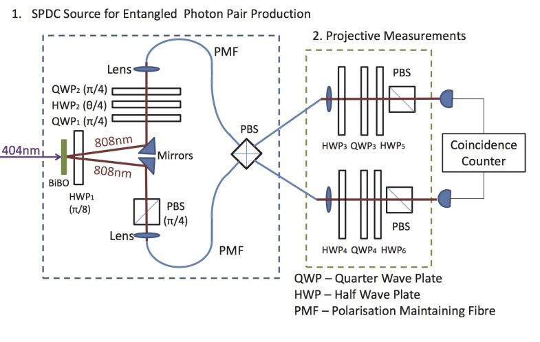
Figure 4: Scheme for polarisation entangled source. Type-I SPDC source is used to generate pairs of H polarised single photons. HWP₁ rotates $\ket{\text{HH}}$ to $\ket{+}\ket{+},\ket{+}=\frac{1}{\sqrt{2}}\ket{\text{H}}\ket{\text{V}}$. The top arm experiences a polarisation-dependent phase shift, and the state of the bottom arm is purified and matched to the top arm by the PBS rotated by $\pi/4$ radians, which transmits $\ket{+}$. The photons are then collected into polarisation maintaining fibres (PMF), where the PBS transmits H and reflects V; in combination with post-selection, the measured state is $\frac{1}{\sqrt{2}}(\ket{\text{HV}}+e^{i\theta}\ket{\text{VH}})$ after renormalisation. Standard tomography set up projects the state onto different bases for measurements. See text for further details.

In order to generate polarisation-entangled photon pairs, a set up similar to matthews2013observing and identical to chapman2016experimental is used. We use the polarisation encoding where $\ket{\mathrm{H}}\equiv\ket{0}$ and $\ket{\mathrm{V}}\equiv\ket{1}$. The set up is shown in Fig.4. A type-I nonlinear crystal (BiBO) is pumped with a vertically polarised cw laser (404 nm) at 80 mW, generating pairs of H polarised single photons (808 nm). The photons are spectrally filtered using 3 nm top-hat filteres centred on 808 nm. The first half way plate HWP₁ (optics axis set to $\pi/8$ radians) rotates the output photon pair from $\ket{\mathrm{HH}}$ to $\ket{\mathrm{++}}$, where $\ket{\mathrm{+}}=\frac{1}{\sqrt{2}}\ket{\mathrm{H}}+\ket{\mathrm{V}}$. The polarisation in the top arm is matched and purified to that of the bottom arm using a polarisation beam splitter (PBS) rotated by $\pi/4$ radians, which transmits $\ket{+}$.

The unitary operation realised by the sequence of wave plates QWP₁ + HWP${}_{2}(\theta)$ + QWP₂, as a function $\theta$ of the HWP₂ angle, applies a phase to photon in V state, effectively that of a phase gate: $\begin{pmatrix}1&0\\ 0&e^{i4\theta}\\ \end{pmatrix}.$ Denoting the the input photon in the top (bottom) arm with subscript 1 (2), the two-photon state collected into the polarisation mainting fibre (PMF) is therefore $\frac{1}{\sqrt{2}}(\ket{\text{H}}_{1}+e^{i\theta}\ket{\text{V}}_{1})\otimes\frac{1}{\sqrt{2}}(\ket{\text{H}}_{2}+\ket{\text{V}}_{2})$.

We use a silicon avalanche single photon counter and measure in coincidence with a time window of 2.5 ns. At the PBS, H is transmitted and V is reflected. After the fibre PBS crystal, the top (bottom) arm fibre contains the components $(\ket{\text{V}}_{1}+\ket{\text{H}}_{2})$ ( $\ket{\text{H}}_{1}+e^{i\theta}\ket{\text{V}}_{2}$). However, the design of the fibre PBS is such that the output coupler flips the polarisation state in the bottom arm, therefore when detected in coincidence, the detector will register either $e^{i\theta}\ket{\text{V}}_{1}\ket{\text{H}}_{2}$ or $\ket{\text{H}}_{2}\ket{\text{V}}_{1}$ , and these two components are made spatially indistinguishable by adjusting the position of the fibre, giving the post-selected state $\frac{1}{\sqrt{2}}(\mathrm{\ket{\text{HV}}+e^{-i\theta}\ket{\text{VH}}})$. HWP₃ and HWP₄ apply the appropriate bit flip operations on each single qubit, and QWP₃+HWP₅ and QWP₄+HWP₆ project the states onto the different bases, which are then measured.

The polarisation maintaining fibres has a beat length (H and V delayed with respect to each other by $2\pi$) of 24mm; the coherence length of the photon pairs is 250 $\mu$m (extracted from a Hong-Ou-Mandel dip of 99$\%$ visibility), which means that if uncompensated, 1.0 m of fibre will spatially separate the H and V components of a photon out of coherence, turning a Bell state $\frac{1}{\sqrt{2}}\ket{\mathrm{HH+VV}}$ into the classically correlated mixture $(\mathrm{\frac{\ket{HH}\bra{HH}+\ket{VV}\ket{VV}}{2}})$. When producing a Bell state, this spatial decoherence was compensated by crossing the slow axis of the PMF and tuning the stage position of the fibre (and vice versa when the mixed state is required).

.1 The Fourier basis

The Fourier basis can be written as single-qubit tensor products in the following way:

$$|f_{j}\rangle=\frac{1}{\sqrt{d}}\bigotimes_{k=0}^{n-1}(|0\rangle+\omega^{j2^{k}}|1\rangle),$$ (S1)

by expressing $k$ in Eq.(4) in binary form. Using equation (4), the maximally entangled state in equation (2) is perfectly correlated (actually, anti-correlated) in this basis:

$$\tfrac{1}{\sqrt{d}}\textstyle{\sum_{j}}|j\rangle|j\rangle=\tfrac{1}{\sqrt{d}}\textstyle{\sum_{k}}|f_{k}\rangle|f_{-k}\rangle.$$ (S2)

.2 The $\sigma_{x}$ basis

The maxiamlly entangled state $\ket{00}+\ket{11}=\ket{++}+\ket{--}$, the mapping (2) can be trivially applied to the $\sigma_{x}$ basis, namely

$$\sum_{j}|j\rangle|j\rangle = (|++\rangle+|--\rangle)^{\otimes n}=\sum_{k}|c_{k}\rangle|c_{k}\rangle,$$ (S3)

showing that the maximally entangled state in equation (2) is maximally correlated also in the $\sigma_{x}$ basis.

.3 Analytical expressions for mutual information

On the state $\rho_{c}$, the joint probabilities for the computational basis is $p(a_{o},b_{o})=\delta_{a_{o}b_{o}}/d$ with $\delta_{ab}$ the Kronecker delta. So the mutual information for the computational basis is $I_{AB}=\log_{2}d$ as expected: there is perfect correlation on such basis in both terms of (6). Writing $\rho_{c}$ in the $\sigma_{x}$ basis, we can calculate the joint probabilities for it as $p(c_{o},d_{o})=\delta_{c_{o},d_{o}}p/d+(1-p)/d^{2}$ (i.e. there is still maximal correlation on the entangled part of $\rho_{c}$, while there is no correlation on the rest). Whence we can calculate $I_{CD}$ and find

$$I_{AB}+I_{CD}=\log_{2}d+$$ (S4)

$$\tfrac{(1-p)(d-1)}{d}\log_{2}(1-p)+\tfrac{1+(d-1)p}{d}\log_{2}(1+(d-1)p).$$

(The same result is obtained also considering the Fourier basis for $CD$ instead of the $\sigma_{x}$ basis.)

Consider now the Werner state $\rho_{w}$. The joint probabilities for the two complementary observables (computational and Fourier bases) are respectively

$$p(a_{o},b_{o})=p/d\delta_{a_{o}b_{o}}+(1-p)/d^{2}\;,$$ (S5)

$$p(c_{o},d_{o})=p/d\delta_{a_{o},-b_{o}}+(1-p)/d^{2}$$ (S6)

$$\Rightarrow I_{AB}+I_{CD}=2I_{AB}=$$ (S7)

$$2\left[\tfrac{1+(d-1)p}{d}\log_{2}[1+(d-1)p]+\tfrac{(1-p)(d-1)}{d}\log_{2}(1-p)\right],$$

which is experimentally determined as the green triangles in Fig.2. The mappings (S2) and (S3), and the fact that $\openone$ remains unchanged in any basis implies that $I_{AB}=I_{CD}$ is the same for all the observables considered here (computational, Fourier and $\sigma_{x}$). Given the symmetry of $\rho_{w}$, our method is able to certify entanglement only for highly-entangled Werner states.

.4 Density matrices

The states used in constructing the family of states as in Eq. (6), (7) and (8) are primarily the Bell states $\frac{1}{\sqrt{2}}(\ket{01}+\ket{10}|),\frac{1}{\sqrt{2}}(\ket{01}-\ket{10}|)$ and the decohered, classically correlated state $\frac{\ket{01}\bra{01}+\ket{10}\bra{10}}{2}$. All the others can be accessed by applying the appropriate local unitary transformation. The density matrices obtained by performing quantum state tomography are shown in Fig.S1,S2 and S3. The fidelities are given in the captions.

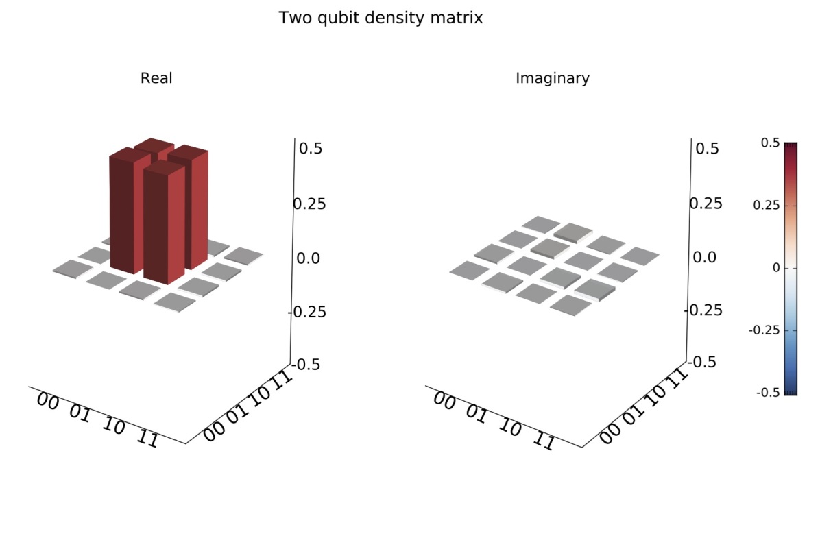
Figure S1: Density matrix for $\frac{1}{\sqrt{2}}(\ket{01}+\ket{10}|)$, fidelity = $97.6\%$ after maximum likelihood [33]

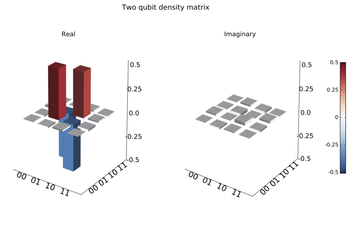
Figure S2: Density matrix for $\frac{1}{\sqrt{2}}(\ket{01}-\ket{10}|)$, fidelity = $97.8\%$ after maximum likelihood.

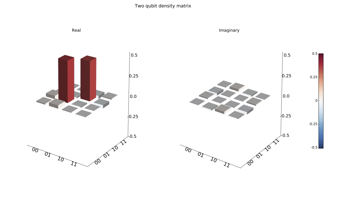
Figure S3: Density matrix for $\frac{\ket{01}\bra{01}+\ket{10}\bra{10}}{2}$, fidelity = $97.6\%$ after maximum likelihood.

.5 $d=2$ states generation

$\rho_{b}$ is generated by averaging measurements for $\ket{\Phi^{+}}\bra{\Phi^{+}}$ with phases applied to a single qubit. $\rho_{s}$ is generated by decohering the Bell-state $\frac{1}{\sqrt{2}}(\ket{00}+e^{i\phi}\ket{11})$ to $\frac{\ket{00}\bra{00}+\ket{11}\bra{11}}{2}$ (See Methods), followed by averaging with the appropriate partial bit flip ($\sigma_{x}\otimes\sigma_{x}$) applied to both qubits. For each value of $p$, 40 iterations were run, the upper and lower bounds of the bands are given by the mean of the 40 points $\pm$ 2 standard deviations respectively. The typical count rates were in the order of 800 coincidences/sec, with accidentals subtracted; for each projective measurement, a 10-second integration time was used such that error due to Poissonian noise would account for $\leq 1\%$ of the measured probability.

$\rho_{w}$ is made by measuring $\ket{\Phi^{+}}\bra{\Phi^{+}}$ and $(\mathbb{I}/4)$ in a time-sharing fashion. All of the states in $d>2$ are generated by combining pure states measurements.

I Data processing and error analysis

Measurement in each MUB involves projecting the state onto a given basis. For each basis projection onto $\rho_{i}$, the counts for that projection is normalised with respect to the normalisation factor ($\mathrm{N_{tot}}$), given : $\mathrm{N_{tot}}=\bra{00}\rho_{i}\ket{00}+\bra{01}\rho_{i}\ket{01}+\bra{10}\rho_{i}\ket{10}+\bra{11}\rho_{i}\ket{11}$

Each statistic was assumed to be a Poissonian process, with standard deviation $\Delta\mathrm{N_{i}}$ = $\sqrt{\mathrm{N_{i}}}$. The error bars displays 2 stdev with the following method of analysis.

$\mathrm{p_{i}=N_{i}/N_{tot}}$, therefore $\mathrm{\Delta p_{i}=p_{i}(\frac{\Delta N_{i}}{N_{tot}}+\frac{\Delta N_{tot}}{N_{tot}}})$ eg. with a total of 10000 counts, the following shows the basis vector, counts for the projection and probability:

$$\begin{pmatrix}HH\\ HV\\ VH\\ VV\end{pmatrix}\rightarrow\begin{pmatrix}1000\\ 4000\\ 4500\\ 500\end{pmatrix}\rightarrow\begin{pmatrix}0.10\\ 0.40\\ 0.45\\ 0.05\end{pmatrix}$$ (S8)

The Shannon entropy for qubit one is given by:

$$\mathrm{H(A)=-p(H)log2(p(H))+p(V)log2p(V)}$$ (S9)

ie

$$\mathrm{H(A)} = -((0.1+0.4)\mathrm{log2}(0.1+0.4)$$ (S10)

$$+(0.45+0.5)\mathrm{log2}(0.45+0.45)$$

$$\begin{split}\mathrm{H(A|B)=-((0.1)log2(\frac{0.1}{0.1+0.45})+(0.45)log2(\frac{0.45}{0.1+0.45})}\\ +\mathrm{(0.40)log2(\frac{0.40}{0.40+0.05})+(0.05)log2(\frac{0.40}{0.40+0.05})}\end{split}$$ (S11)

The error in the probabilities are therefore:

$$\Delta p_{i}=\begin{pmatrix}0.1(\frac{\sqrt{1000}}{1000}+\frac{\sqrt{10000}}{10000})\\ 0.40(\frac{\sqrt{4000}}{4000}+\frac{\sqrt{10000}}{10000})\\ 0.45(\frac{\sqrt{4500}}{4500}+\frac{\sqrt{10000}}{10000})\\ 0.05(\frac{\sqrt{500}}{500}+\frac{\sqrt{10000}}{10000})\end{pmatrix}$$ (S12)

$$\mathrm{I}=-\sum_{i}\mathrm{p_{i}log_{2}(p_{i})}$$ (S13)

At each point displayed on the graphs in the main text, the error bars were calculated via error propagation. The uncertainty in information, $\Delta I$ then follows as:

$$\mathrm{\Delta I}=-\mathrm{\frac{1}{ln(2)}\sum_{i}(\Delta p_{i}ln(p_{i})+p_{i}\Delta(ln(p_{i})))}\$$ (S14)

$$=-\mathrm{\frac{1}{ln(2)}\sum_{i}(\Delta p_{i}ln(p_{i})+1))}$$ (S15)

II Maximal MUB’s in $d=3$ and 4

We used the MUB’s from [34] to perform our calculations. Note that for d = 4, out of the four sets of MUB’s provided, there is an error in that the two sets are identical. We amended this, and the ones we used are specified in Eq.(LABEL:eq:fourMUBs)

For $d=3$:

$$\{\ket{F3_{a}}\} = \{\frac{1}{3}[1,1,1],\frac{1}{3}[1,\omega,\omega^{2}],\frac{1}{3}[1,\omega^{2},\omega]\}$$

$$\{\ket{F3_{b}}\} = \{\frac{1}{3}[1,\omega,\omega],\frac{1}{3}[1,\omega^{2},1],\frac{1}{3}[1,1,\omega^{2}]\}$$

$$\{\ket{F3_{c}}\} = \{\frac{1}{3}[1,\omega^{2},\omega^{2}],\frac{1}{3}[1,\omega,1],\frac{1}{3}[1,1,\omega]\}$$ (S16)

where $\omega=e^{2\pi i/d}$. Together with the computational basis, these form the four sets of MUB’s in $d=3$.

For the computational and the Fourier basis ($\{\ket{F3_{a}}\}$), maximal correlation occur when the two systems are measured in these the same respective bases. For $\{\ket{F3_{b}}\}$ and $\{\ket{F3_{c}}\}$ however, there is zero correlation if both sides are measured in the same bases. To achieve maximum correlation, when system one is measured in $\{\ket{F3_{b}}\}$ ( $\{\ket{F3_{c}}\}$), system two must be measured with a different set of MUB as defined in Eqn.(S17) ((S18)).

Comparing the mutual information for using just two MUB’s (red dotted) and the full four MUB’s, are given in Fig.S4.

$$\{\frac{1}{3}[\omega,1,1],\frac{1}{3}[1,1,\omega],\frac{1}{3}[1,\omega,1]\}$$ (S17)

$$\{\frac{1}{3}[\omega^{2},1,1],\frac{1}{3}[1,1,\omega^{2}],\frac{1}{3}[1,\omega^{2},1]\}$$ (S18)

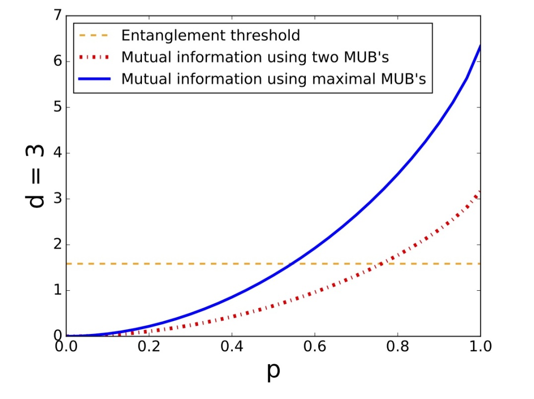
Figure S4: Mutual information of the Werner state in Eqn (7) for $d=3$ when measured in only two MUB’s (red dotted line), or all five sets of MUB’s (blue solid line)

For $d=4$, we used the following bases:

$$\{\ket{F4_{a}}\} = \{\frac{1}{2}[1,1,1,1,],\frac{1}{2}[1,1,-1,-1],$$

$$\frac{1}{2}[1,-1,-1,1],\frac{1}{2}[1,-1,1,-1]\}$$

$$\{\ket{F4_{b}}\} = \{\frac{1}{2}[1,-1,-i,-i],\frac{1}{2}[1,-1,i,i],$$

$$\frac{1}{2}[1,1,i,-i],\frac{1}{2}[1,1,-i,i]\}$$

$$\{\ket{F4_{c}}\} = \{\frac{1}{2}[1,-i,-i,-1],\frac{1}{2}[1,-i,i,1],$$

$$\frac{1}{2}[1,i,i,-1],\frac{1}{2}[1,i,-i,1]\}$$

$$\{\ket{F4_{d}}\} = \{\frac{1}{2}[1,-i,1,-i],\frac{1}{2}[1,-i,1,i],$$ (S19)

$$\frac{1}{2}[1,i,1,-i],\frac{1}{2}[1,i,-1,i]\}$$

Together with the computational basis, these form the five sets of MUB’s in $d=4$. The mutual information for the Werner state, when measured using two MUB’s (red dotted) and the full five MUB’s, are given in Fig.S5.

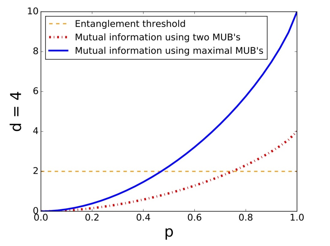
Figure S5: Mutual information of the Werner state in Eqn (7) for $d=4$ when measured in only two MUB’s (red dotted line), or all five sets of MUB’s (blue solid line)

References

- (1) Arndt, M. & Hornberger, K. Testing the limits of quantum mechanical superpositions. Nat. Phys. 10, 271–277 (2014).
- (2) Sciarrino, F. Quantum optics: Micro meets macro. Nat. Phys. 9, 529–529 (2013).
- (3) Friedman, J. R., Patel, V., Chen, W., Tolpygo, S. & Lukens, J. E. Quantum superposition of distinct macroscopic states. Nat. 406, 43–46 (2000).
- (4) Gühne, O. et al. Detection of entanglement with few local measurements. Phys. Rev. A 66, 062305 (2002).
- (5) Artiles, L., Gill, R. et al. An invitation to quantum tomography. J. Roy. Statist. Soc. Ser. B 67, 109–134 (2005).
- (6) Mair, A., Vaziri, A., Weihs, G. & Zeilinger, A. Entanglement of the orbital angular momentum states of photons. Nat. 412, 313–316 (2001).
- (7) Bennett, C. H. & Wiesner, S. J. Communication via one- and two-particle operators on Einstein-Podolsky-Rosen states. Phys. Rev. Lett. 69, 2881–2884 (1992).
- (8) Bruß, D. & Macchiavello, C. Optimal eavesdropping in cryptography with three-dimensional quantum states. Phys. Rev. Lett. 88, 127901 (2002).
- (9) Durt, T., Kaszlikowski, D., Chen, J.-L. & Kwek, L. C. Security of quantum key distributions with entangled qudits. Phys. Rev. A 69, 032313 (2004).
- (10) Bruß, D. Characterizing entanglement. J. Math. Phys. 43, 4237–4251 (2002).
- (11) Horodecki, R., Horodecki, P., Horodecki, M. & Horodecki, K. Quantum entanglement. Rev. Mod. Phys. 81, 865–942 (2009).
- (12) Gühne, O. & Tóth, G. Entanglement detection. Phys. Rep. 474, 1 – 75 (2009).
- (13) Gühne, O. et al. Experimental detection of entanglement via witness operators and local measurements. J. Modern Opt. 50, 1079–1102 (2003).
- (14) Kothe, C. & Björk, G. Entanglement quantification through local observable correlations. Phys. Rev. A 75, 012336 (2007).
- (15) Abascal, I. S. & Björk, G. Bipartite entanglement measure based on covariance. Phys. Rev. A 75, 062317 (2007).
- (16) Maccone, L., Bruß, D. & Macchiavello, C. Complementarity and correlations. Phys. Rev. Lett. 114, 130401 (2015).
- (17) Maassen, H. & Uffink, J. B. M. Generalized entropic uncertainty relations. Phys. Rev. Lett. 60, 1103–1106 (1988).
- (18) Schneeloch, J., Broadbent, C. J. & Howell, J. C. Uncertainty relation for mutual information. Phys. Rev. A 90, 062119 (2014).
- (19) Coles, P. J. & Piani, M. Improved entropic uncertainty relations and information exclusion relations. Phys. Rev. A 89, 022112 (2014)
- (20) Coles, P. J., Colbeck, R., Yu, L. & Zwolak, M. Uncertainty relations from simple entropic properties. Phys. Rev. Lett. 108, 210405 (2012).
- (21) Coles, P. J. & Piani, M. Complementary sequential measurements generate entanglement. Phys. Rev. A 89, 010302 (2014).
- (22) Fickler, R. et al. Quantum entanglement of high angular momenta. Sci. 338, 640–643 (2012).
- (23) Dada, A. C., Leach, J., Buller, G. S., Padgett, M. J. & Andersson, E. Experimental high-dimensional two-photon entanglement and violations of generalized bell inequalities. Nat. Phys. 7, 677–680 (2011).
- (24) Zheng, S.-B. Generation of entangled states for many multilevel atoms in a thermal cavity and ions in thermal motion. Phys. Rev. A 68, 035801 (2003).
- (25) Ye, S.-Y., Zhong, Z.-R. & Zheng, S.-B. Deterministic generation of three-dimensional entanglement for two atoms separately trapped in two optical cavities. Phys. Rev. A 77, 014303 (2008).
- (26) Lo, H.-P. et al. Experimental violation of bell inequalities for multi-dimensional systems. arXiv preprint arXiv:1501.06429 (2015).
- (27) Collins, D., Gisin, N., Linden, N., Massar, S. & Popescu, S. Bell inequalities for arbitrarily high-dimensional systems. Phys. Rev. Lett. 88, 040404 (2002).
- (28) Kendon, V. M., Życzkowski, K. & Munro, W. J. Bounds on entanglement in qudit subsystems. Phys. Rev. A 66, 062310 (2002).
- (29) Ollivier, H. & Zurek, W. H. Quantum discord: A measure of the quantumness of correlations. Phys. Rev. Lett. 88, 017901 (2001).
- (30) Matthews, J. C. et al. Observing fermionic statistics with photons in arbitrary processes. Sci. Rep. 3, 1539 (2013).
- (31) James, D. F. V., Kwiat, P. G., Munro, W. J. & White, A. G. Measurement of qubits. Phys. Rev. A 64, 052312 (2001).
- (32) Klappenecker, A. & Rötteler, M. Constructions of mutually unbiased bases. In Finite fields and applications, 137–144 (Springer, 2004).
- (33) Chapman, R. J. et al. Experimental perfect quantum state transfer. arXiv:1603.00089 (2016).