Trading-Off Cost of Deployment Versus Accuracy in Learning Predictive Models

Abstract

Predictive models are finding an increasing number of applications in many industries. As a result, a practical means for trading-off the cost of deploying a model versus its effectiveness is needed. Our work is motivated by risk prediction problems in healthcare. Cost-structures in domains such as healthcare are quite complex, posing a significant challenge to existing approaches. We propose a novel framework for designing cost-sensitive structured regularizers that is suitable for problems with complex cost dependencies. We draw upon a surprising connection to boolean circuits. In particular, we represent the problem costs as a multi-layer boolean circuit, and then use properties of boolean circuits to define an extended feature vector and a group regularizer that exactly captures the underlying cost structure. The resulting regularizer may then be combined with a fidelity function to perform model prediction, for example. For the challenging real-world application of risk prediction for sepsis in intensive care units, the use of our regularizer leads to models that are in harmony with the underlying cost structure and thus provide an excellent prediction accuracy versus cost tradeoff.

1 Introduction

Many industries (e.g., retail, manufacturing, and medicine) are recognizing the advantages of using predictive models to make key decisions. They also understand that the cost of obtaining input measurements should be balanced with their effectiveness in prediction when choosing which model to deploy. This is especially challenging when the cost structure for an application is complicated. As an important example, consider the cost structure associated with deploying a predictive model in an Intensive Care Unit (ICU) (see the cost-dependency graph in Figure 1). In such a setting, the following hold: (i) costs may be defined for tests, measurements, or activities and these costs may be of different types (e.g., the financial cost of acquiring a blood test versus the staff time taken to draw blood); (ii) features are obtained using one or more measurements (e.g., lactate level or creatinine) which in turn are obtained by ordering a test; (iii) a test may consist of a single measurement (e.g., lactate level) or a panel of measurements (e.g., CBC panel); (iv) a measurement can be ordered via multiple tests (e.g., creatinine can be ordered on its own, as part of a basic or a comprehensive metabolic panel, each having a different financial cost); (v) multiple features can be derived from the same measurement (e.g., the heart rate variability and the heart rate trend can both be derived from the heart rate trace); and (vi) some features may require multiple measurements (e.g., shock index is derived from blood pressure and heart rate measurements). These aspects make the cost structure complicated.

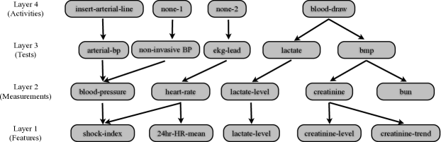
Figure 1: A portion of the dependency graph for the ICU example.

Before expanding upon the challenges involved with addressing complex cost-structures such as the one above, we first introduce the mathematical setup for learning predictive models. This involves data that is formally represented by sets of pairs $\{(x_{i},y_{i})\}_{i=1}^{N}$ for some integer $N$, where $x_{i}\in\Re^{n}$ for some integer $n$ and $y_{i}\in\Re$, for all $1\leq i\leq N$. The vector $x_{i}$ denotes the $i$th input (feature) vector and $y_{i}$ the output (label) associated with the $i$th input vector $x_{i}$. The goal is then to predict the unknown output associated with a newly obtained input vector by using the knowledge one learns from the data $\{(x_{i},y_{i})\}_{i=1}^{N}$. A popular approach for performing this task is to build predictive models via empirical regularized-loss minimization Vapnik (1998). The problems used take the form

$${\displaystyle\mathop{\operator@font{minimize}}_{\beta\in\Re^{n}}}\;\;f(\beta):=\frac{1}{N}\sum_{i=1}^{N}L\big{(}\beta;(x_{i},y_{i})\big{)}+R(\beta),$$ (1)

where $\beta\in\Re^{n}$ is the parameter vector to be learned, $L$ is a loss function such as the logistic loss $L(\beta;(x_{i},y_{i}))=\log(1+\exp^{y_{i}x_{i}^{T}\!\beta})$, and $R$ is a regularizer. The choice of regularizer amounts to giving preference to certain models, e.g., the $\ell_{1}$-regularizer $R(\beta)=\lambda\|\beta\|_{1}$ for some $\lambda>0$ prefers models defined by a sparse vector $\beta$. In practice, the regularizer should be chosen to reflect the preferred models, which are often driven by the costs associated with the application. For example, in compressed sensing, one wishes to find a sparse solution to a linear system of equations. Thus, the cost, i.e., the number of nonzeros in a prospective solution, is harmonious with the $\ell_{1}$-regularizer, which promotes sparse solutions. Note that in this example, as well as many others, the costs are directly tied to the feature vectors themselves, i.e., they occur at the feature level.

How does one design an appropriate regularizer for problems with a complicated cost structure, such as for the ICU example above? We address that question in this paper.

Related work. Learning models in the presence of costs has received significant attention in recent years (e.g., Xu et al. (2012); Ji and Carin (2007); Weiss and Taskar (2013); Xu et al. (2013); Raykar et al. (2010)). Existing work has primarily targeted applications where the cost of computation is the primary concern, and this cost is elicited at the feature level. Moreover, much of this work has focused on optimizing performance when information is acquired incrementally Ji and Carin (2007); Xu et al. (2012); Trapeznikov and Saligrama (2013); Kanani and Melville (2008); Kapoor and Horvitz (2009). In Ji and Carin (2007), they define the problem of cost-sensitive classification and use a partially observable Markov decision process to trade-off the cost of acquiring additional measurements with classification performance. While they apply their method to a medical diagnosis problem, their costs were approximated at the feature level. In Xu et al. (2012), stage-wise regression is used to learn a collection of regression trees in a manner that ensures that classifiers built from more trees is more accurate, but more expensive. For the task of ranking web page documents, they showed improved speed and accuracy by accounting for feature costs—simple lookups (e.g., word occurrences) versus those needing more computation (e.g., a document-specific BM25 score for measuring relevance to a query). For structured prediction, Weiss et al. (2013) proposed a two tier collection of models of varying costs and a model selector; for each new test example, their selector adaptively chooses a model. For vision applications (e.g., articulated pose estimation in videos), they showed gains in performance by adaptively selecting models of varying costs by using a histogram of gradient features at a fine (expensive) versus a coarse (cheap) resolution. These solutions focused on applications with no dependencies between the costs for the units reasoned over (i.e. feature or model costs are independent) and when they are provided upfront. As predictive models continue to find their way into many important applications, a means for incorporating rich cost structures is needed.

Returning to our example in healthcare, the challenge of incorporating costs arises from the dependencies between features, measurements, tests, and required activities. Measurements may be obtained from a singleton test or as part of a test that yields multiple measurements. Tests may have different resource costs associated with them, while features may be derived from more than one measurement. These dependencies between features, measurements and tests yield a complex dependence structure between the features. Moreover, various costs are specified at different levels of this hierarchy; therefore, the cost of a feature is not specified upfront, but rather is dependent on which other features, measurements, and tests are selected.

Cost imposed via a hierarchical dependency graph is reminiscent of past works utilizing structured sparsity penalties (see the survey Wainwright (2014) and Bach et al. (2012)), especially those using tree-based regularizers Kim and Xing (2010) and penalties with overlapping groups and hierarchical structure Zhao et al. (2006); Bach et al. (2012). Different from these past works, a key challenge for our task is that the structure of the group regularizer is not given and its construction is not straightforward. We show that cost-dependency graphs are naturally captured via Boolean circuits—graphs where nodes share a combination of AND and OR connections with its parents. Only leaf nodes (i.e. feature nodes) of this circuit are included in the regularizer while the internal nodes (e.g., measurements needed to obtain features) induce dependency between the leaf nodes. The presence of mixed AND/OR relationships and the non-inclusion of internal nodes renders our application different from past works. Other regularizers such as OSCAR Zhong and Kwok (2012) and Laplacian Net Huang et al. (2011) aim at discovering group structure when the features are highly correlated. In our setting, the groups are determined by the structure of the cost graph, not by the correlations between the features.

Our contributions. We develop a new framework for defining structured regularizers suitable for problems with complex cost structures by drawing upon a surprising connection to boolean circuits. In particular, we represent the problem costs as a boolean circuit, and then use properties of boolean circuits to define the exact cost penalty. Based on our exact cost penalty, any standard convex relaxation may be employed for the purpose of computational efficiency, and here we choose a standard $\ell_{1}$-$\ell_{\infty}$ relaxation. Our new regularizer may be used within an empirical risk minimization framework to tradeoff cost versus accuracy. We focus on the one-shot setting (i.e., when all measurements are obtained upfront), although our regularizer is also applicable in the incremental setting. Since the cost-structure of many real-life applications may be represented as a boolean circuit, the contribution of our work is substantial.

Our ideas are presented in the context of a challenging healthcare application—the development of a rapid screening tool for sepsis Angus and van der Poll (2013)—using data from patients in the ICU Saeed et al. (2011). In this setting, examples of potential users include patients, doctors, and administration. Our experiments show that our regularizer allows for a collection of models that are in harmony with a user’s cost preferences. Numerical comparisons to a cost-sensitive $\ell_{1}$—a natural competitor to our proposed regularizer that does not account for the complicated cost structure—shows that models obtained with our regularizer have a better prediction/cost tradeoff. Compared to existing approaches in predictive modeling where cost preferences are often accounted for post hoc, our scheme provides a new way to account for complex cost preferences during model selection.

2 Regularizers for complex cost structures

Our scheme is general since it may be applied to any problem with a cost structure that may be represented as a finite-layer boolean circuit. However, for clarity of exposition, we first focus on a particular healthcare application that also serves as the basis for the numerical results presented.

2.1 An example from the intensive-care unit (ICU)

We formulate a structured regularizer for the cost structure associated with risk prediction applications for the in-hospital setting. These include problems such as prediction of those at risk for death, the likelihood of readmission, and the early detection of adverse events, e.g., shock and cardiac arrest.

Recall the cost dependency graph for the ICU example in Figure 1. The features are represented by nodes in layer-$1$, and their calculation requires a subset of measurements from layer $2$, i.e., nodes in layer-$1$ share an AND or OR relationship with those in layer-$2$. Measurements can be obtained in a number of ways by performing various tests, which are represented at layer-$3$, i.e., nodes in layer-$2$ similarly share an AND or OR relationship with those in layer-$3$. The caregiver activities are represented at layer-$4$ and are performed when a test is needed that requires that action, i.e., layer-$3$ shares an AND relationship with layer-$4$. Every relationship in this boolean circuit is described using only logical AND and OR operations. Note that, without loss of generality, we include fictitious nodes “none-1” and “none-2” in layer-$4$ so that the collection of input nodes are in the same layer.

There are three relevant costs: the financial cost of ordering a test, the waiting time to obtain a test result, and the caregivers’ time needed to perform the activities required for the tests. The ideal regularizer should account for the following: (i) obtaining a measurement may cost different amounts depending on which tests are ordered to obtain it; (ii) features share costs with other features derived from the same measurement; (iii) a feature may require multiple measurements so that its cost depends on more than one measurement; and (iv) caregiver time and financial costs are additive while wait time is the maximum of the separate wait times.

Our structured regularizer requires the following sets:

$$\mathcal{F} :=\{f_{1},\cdots,f_{n_{f}}\},\;\; \;\;\;\mathcal{M} :=\{m_{1},\cdots,m_{n_{m}}\},\;\;$$

$$\mathcal{T} :=\{t_{1},\cdots,t_{n_{t}}\},\;\; \mathcal{A} :=\{a_{1},\cdots,a_{n_{a}}\}.$$

to be the sets of features (layer-$1$ nodes), measurements (layer-$2$ nodes), tests (layer-$3$ nodes), and caregiver activities (layer-$4$ nodes), with $n_{f},n_{m},n_{t},$ and $n_{a}$ being the number of each, respectively. We use $f_{i}\hookleftarrow m_{i}$ to mean that there is a directed edge that links node $m_{j}$ to node $f_{i}$. Thus, our specific boolean circuit allow us to interpret $f_{i}\hookleftarrow m_{j}$, $m_{j}\hookleftarrow t_{k}$, and $t_{k}\hookleftarrow a_{l}$ to mean the $i$th feature requires the $j$th measurement, the $j$th measurement can be obtained by performing the $k$th test, and the $k$th test requires the $l$th activity.

We now define the set valued mappings $m(f_{i}):=\{m_{j}:f_{i}\hookleftarrow m_{j}\}$, $t(m_{j}):=\{t_{k}:m_{j}\hookleftarrow t_{k}\}$, and $t(a_{l}):=\{t_{k}:t_{k}\hookleftarrow a_{l}\}$, which represent the set of measurements required to obtain feature $i$, the set of tests that produce measurement $j$, and the set of tests that require action $l$. We note that we have overloaded the definition of the function $t$ above, i.e., we have two different definitions for $t(m_{j})$ and $t(a_{l})$. However, this should not lead to any confusion since the correct definition is always clear from the context.

Next, we resolve the fact that some features may be obtained in multiple ways by ordering various combinations of tests. If this is not considered, the cost of a feature may be over penalized by our regularizer. To address this issue, let $w_{i}$ denote the numbers of ways feature $i$ can be obtained. Then, for the $i$th feature, we define $\vec{f}_{i}:=[f_{i,1},\cdots,f_{i,w_{i}}]^{T}$ and $\vec{\beta}_{i}:=[\beta_{i,1},\cdots,\beta_{i,w_{i}}]^{T}$ so that $\beta_{i,p}$ represents the parameter associated with ordering feature $f_{i}$ in the $p$th way. This allows us to define the extended feature and parameter vectors $\vec{f}:=[\vec{f_{1}},\dots,\vec{f_{n_{f}}}]^{T}$ and $\vec{\beta}:=[\vec{\beta_{1}},\dots,\vec{\beta_{n_{f}}}]^{T}$.

Modeling financial cost and caregiver time: To model financial cost, which is incurred at the test level, for each test $t_{k}$ and feature $f_{i}$ we define $\vec{n}_{k,i}:=[n_{k,i,1},\cdots,n_{k,i,w_{i}}]^{T}$ with

$$n_{k,i,p}:=\!\begin{cases}1&\!\mbox{if $t_{k}$ is used when $f_{i}$ is ordered in its $p$th way,}\\ 0&\!\mbox{otherwise,}\end{cases}$$

for all $1\leq k\leq n_{t}$, $1\leq i\leq n_{f}$, and $1\leq p\leq w_{i}$. Given a financial cost $C_{k}^{\mathcal{T}}$ of ordering test $k$ and a weighting parameter $\lambda_{\$}$, the exact structured regularizer for financial cost is

$$R_{exact}^{\$}(\vec{\beta}):=\lambda_{\$}\!\sum_{k=1}^{n_{t}}\mathcal{C}_{k}^{\mathcal{T}}I\!\left(\sum_{i=1}^{n_{f}}\sum_{p=1}^{w_{i}}I(n_{k,i,p}\beta_{i,p})\right)$$ (2)

with the indicator function $I$ satisfying $I(0)=0$ and $I(z)=1$ for all $z\neq 0$. It follows from (2) that a financial cost for test $t_{k}$ is incurred only when instructed to order some feature $f_{i}$ in the $p$th way ($\beta_{i,p}\neq 0$), and that $p$th way requires test $t_{k}$ ($n_{k,i,p}\neq 0$). The regularizer (2) is not computationally friendly, so we instead use the relaxed structured regularizer

$$R_{relax}^{\$}(\vec{\beta}) :=\lambda_{\$}\!\sum_{k=1}^{n_{t}}\mathcal{C}_{k}^{\mathcal{T}}\Big{\|}\bigvee_{i=1}^{n_{f}}\vec{n}_{k,i}\odot\vec{\beta}_{i}\Big{\|}_{\infty}$$ (3)

where we define for a set of vectors $\{z_{i}\}_{i=1}^{n}$ and a subset $S=\{i_{1},i_{2},\dots,i_{r}\}\subseteq\{1,2,\dots,n\}$ the quantities

$$\bigvee_{i=1}^{n}z_{i}:=[z_{1}^{T}\dots z_{n}^{T}]^{T}\;\;\text{and}\;\;\bigvee_{i\in{\mathcal{S}}}z_{i}:=[z_{i_{1}}^{T}\dots z_{i_{r}}^{T}]^{T}.$$

Note that (3) is a sum of group $\ell_{\infty}$-norms, which is supported by the software SPAMS.

To model the caregivers time cost in a similar way, we define $\vec{n}_{l,i}:=[n_{l,i,1},\cdots,n_{l,i,w_{i}}]^{T}$ with

$$n_{l,i,p}:=\!\begin{cases}1&\!\mbox{if $a_{l}$ is used when $f_{i}$ is ordered in its $p$th way,}\\ 0&\!\mbox{otherwise,}\end{cases}$$

for all $1\leq l\leq n_{a}$, $1\leq i\leq n_{f}$, and $1\leq p\leq w_{i}$, where we have again overloaded notation. The regularizer associated with caregiver activity time then becomes

$$R_{relax}^{time}(\vec{\beta}) :=\lambda_{time}\!\sum_{l=1}^{n_{a}}\mathcal{C}_{l}^{\mathcal{A}}\Big{\|}\bigvee_{i=1}^{n_{f}}\vec{n}_{l,i}\odot\vec{\beta}_{i}\Big{\|}_{\infty}$$ (4)

with $\mathcal{C}_{l}^{\mathcal{A}}$ being the time cost associated with the $l$th activity and $\lambda_{time}>0$ a weighting parameter. Overall, our structured regularizer becomes

$$R_{relax}(\vec{\beta}):=R_{relax}^{\$}(\vec{\beta})+R_{relax}^{time}(\vec{\beta}).$$ (5)

By varying $\lambda_{\$}$ and $\lambda_{time}$ we trade-off the financial and caregiver activity time costs, respectively.

Remark 1

If a scaled-$\ell_{1}$-norm was used, the user chooses a weight for each feature by condensing the complex cost structure into a single number, necessarily in an ad-hoc way.

Remark 2

Consider the $3$-layer boolean circuit where layer-$1$ contain the nodes ${\mathcal{F}}$, layer-$2$ contain the nodes $\mathcal{Z}:=\{f_{i,p}:1\leq i\leq n_{f}\ \text{and}\ 1\leq p\leq w_{i}\}$, and layer-$3$ contain the nodes ${\mathcal{A}}$. Moreover, the gate functions at layer-$1$ are given, for each $f_{i}$, by $g_{f_{i}}(\mathcal{Z}):=\underset{1\leq p\leq w_{i}}{{\rm OR}}f_{i,p}$ for all $1\leq i\leq n_{f}$, and the gate functions at layer-$2$ are given, for each $f_{i,p}$, by $g_{f_{i,p}}({\mathcal{A}}):=\underset{\{l:n_{l,i,p}=1\}}{{\rm AND}}a_{l}$ for all $1\leq i\leq n_{f}$ and $1\leq p\leq w_{i}$. In particular, only OR gate functions are used in layer-$1$ and only AND gate functions are used in layer-$2$. Moreover, the properties of this $3$-layer gate allows us to conclude that for a given caregiver activity, say $a_{l}$, we have $\left\|\bigvee_{i=1}^{n_{f}}\vec{n}_{l,i}\odot\vec{\beta}_{i}\right\|_{\infty}\equiv\left\|\bigvee_{(i,p)\in{\mathcal{S}}_{l}}\vec{\beta}_{i,p}\right\|_{\infty}$ with the index set ${\mathcal{S}}_{l}$ defind as ${\mathcal{S}}_{l}:=\{(i,p):n_{l,i,p}=1\}=\{(i,p):\,\text{the output of $g_{f_{i,p}}(\cdot)$ depends on $a_{l}$}\}$, so that the definition of our regularizer (4) follows from our knowledge of the $3$-layer boolean circuit. In fact, the only properties of the circuit that we used were (i) layer-$1$ was the feature layer; (ii) layer-$3$ contained the nodes whose costs we were modeling; (iii) layer-$1$ only contained OR gates; and (iv) layer-$2$ only had AND gates. This motivates the general case below.

Modeling testing wait time: We use a simpler approach to address the time needed to obtain test results. Note that the wait time for a set of test results is the maximum of the wait times for each individual test (assuming that tests can be ordered in parallel). Thus, for a given upper bound, say $W$, on the tolerated testing wait time, we only allow tests that have a wait time less than $W$ to be used. This amounts to selecting a reduced boolean circuit containing only these allowed tests, the caregiver actions required to obtain these allowed tests, measurements that result from the allowed tests, and the features that may be calculated from the included measurements.

2.2 Structured regularizer: the general case

We now show how to define our regularizer for any problem whose cost structure may be represented as a finite $r$-layer boolean circuit; Figure 1 is an instance of such a circuit.

An $r$-layer boolean circuit consists of layers of finitely many nodes. The lowest layer (layer-$1$) consists of the set of output nodes, while the highest layer (layer-$r$) contains the input nodes. Additionally, we are given boolean functions—defined on the basis ${\mathcal{B}}=\{{\rm AND},{\rm OR},{\rm NOT}\}$—for all nodes. Formally, each boolean function performs the basic logical operations from ${\mathcal{B}}$ on one or more logical inputs from the previous layer, and produces a single logical output value. The healthcare example in Figure 1 is a $4$-layer boolean circuit with the features corresponding to layer-$1$, the measurements to layer-$2$, the tests to layer-$3$, and the activities to layer-$4$.

Let ${\mathcal{N}}_{i}:=\{x_{i,1},x_{i,2},\dots,x_{i,n_{i}}\}$ be the nodes in layer-$i$ for some $n_{i}$. By removing double negations, and using the laws of distribution and De Morgan’s laws, the $r$-layer circuit may be reduced to a $3$-layer boolean circuit in disjunctive normal form Pfahringer (2010); Zeng et al. (2012). The nodes in the $3$-layer circuit are then layer-$3$: $\{x_{r,1},x_{r,2},\dots,x_{r,n_{r}}\}$, layer-$2$: $\{z_{1},z_{2},\dots,z_{m}\}$, and layer-$1$: $\{x_{1,1},x_{1,2},\dots,x_{1,n_{1}}\}$ for some $m$ and set $\{z_{i}\}_{i=1}^{m}$ of nodes for layer-$2$. Moreover, the only logical operations used by the boolean functions $g_{z_{i}}(\cdot)$ in layer-2 are AND and NOT operations, while the boolean functions $g_{x_{1,i}}(\cdot)$ in layer-$1$ only use logical OR operations. (In Remark 2 we showed how a circuit of this form could be obtained for the healthcare example.) If we define the vectors $\vec{z}:=[z_{1},z_{2},\dots,z_{m}]^{T}$ and $\vec{\beta}:=[\beta_{1},\beta_{2},\dots,\beta_{m}]^{T}$, then we define our cost-driven structured regularizer as

$$R_{relax}(\,\vec{\beta}\,):=\lambda\!\sum_{k=1}^{n_{r}}\mathcal{C}_{k}\Big{\|}\bigvee_{j\in{\mathcal{S}}_{k}}\beta_{j}\Big{\|}_{\infty}$$

with ${\mathcal{S}}_{k}:=\{j:g_{z_{j}}(\cdot)\,\text{depends on the logical value of}\,x_{r,k}\}$. When this regularizer is used in model prediction, an optimal value for the extended vector $\vec{\beta}$ is obtained. Using this vector and the fact that layer-$1$ only has OR gates, we know that a node $x_{1,i}$ in layer-$1$ (i.e., the feature layer for the healthcare application) has the logical value of $1$ (i.e., the feature should be computed) if $\beta_{j}\neq 0$ for some $j\in\{k:g_{x_{1,i}}(\cdot)\ \text{depends on the logical value of}\ z_{k}\}$.

Remark 3

Although our exact penalty is approximated by an overlapping group regularizer, what is non-trivial is determining which features belong to which groups for complex cost graphs. By relating the cost graph to a Boolean circuit, we can use properties of Boolean circuits to define an extended feature set and overlapping structure that is correct for arbitrary cost graphs. Moreover, this connection allows for the use of widely used off-the-shelf software such as SymPy to convert an arbitrary graph to the 3-layer circuit in disjunctive normal form used to define our exact regularizer.

3 Numerical experiments

We focus on early detection of septic shock—an adverse event resulting from sepsis—since it is the 11th leading cause of patient mortality in the United States. (Mortality rates are between $30\%$ and $50\%$ for those who develop septic shock Angus et al. (2001).) Although early treatment can reduce the patient mortality rate, less than one-third of patients receive appropriate therapy before onset. Therefore, an early warning system that accurately predicts a sepsis event allows for appropriate treatment and a higher quality of patient care. (See the references in Ho et al. (2014) for recent work on sepsis detection; none have tackled the cost of deployment.) More broadly, this problem is an instance of cost-sensitive risk prediction for automated triage Wilson et al. (1981).

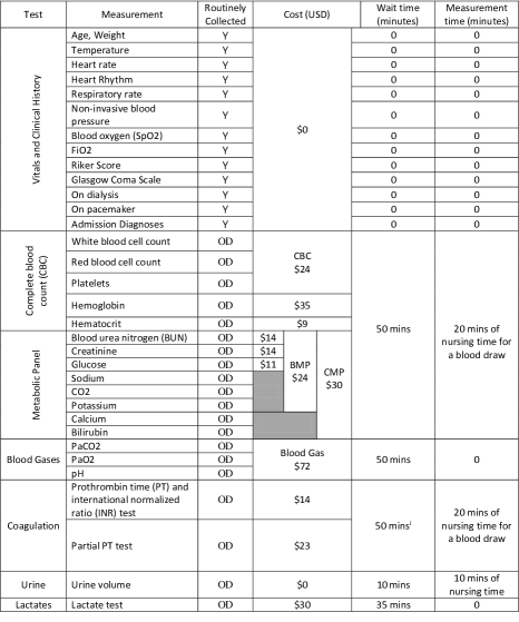
Figure 2: The cost structure (measurements and associated costs) for risk prediction of adverse events in an ICU. Some measurements are made on demand (OD), while the others are routinely collected. The following acronyms are used: basic metabolic panel (BMP), comprehensive metabolic panel (CMP), and complete blood count (CBC).

Table 1: Various costs for different models obtained by using our structured regularizer.

Models	$\mathcal{M}_{1}$	$\mathcal{M}_{2}$	$\mathcal{M}_{3}$	$\mathcal{M}_{4}$
Sensitivity at $0.85$ specificity	0.61	0.66	0.65	0.72
AUC	$82.79\pm 0.55$	$84.45\pm 0.64$	$84.75\pm 0.55$	$87.21\pm 0.46$
Financial Cost	$$0$	$$0$	$$72$	$$170$
Caregiver Time	0 minutes	$10$ minutes	0 minutes	$30$ minutes
Result Time	0 minutes	$10$ minutes	50 minutes	$50$ minutes
Tests Required	routine	routine, urine	abg, routine	abg, cbc, cmp, hct, hemoglobin, routine, urine
Activities Required	none	urine	arterial stick	arterial stick, blood draw, urine

We constructed the full cost-graph in collaboration with domain experts, which resulted in $119$ nodes and $294$ edges. (The full list of measurements and tests can be found in Figure 2.) We combine the logistic-regression function with our structured regularizer (5) to predict the probability that a patient will develop septic shock. We use MIMIC-II Saeed et al. (2011), a large publicly available dataset of electronic health records from patients admitted to four different ICUs at the Beth Israel Deaconess Medical Center over a seven year period. Using the processing described in Henry et al. (2015), $2,\!291$ positive patients and $12,\!646$ negative patient cases were obtained.

We answer two questions. Does our structured regularizer lead to diverse models, especially in terms of the various costs? How well does our new structured regularizer perform compared to existing available solutions? Natural comparisons include regularizers that account for cost but do not account for the cost-dependence structure, e.g., the $\ell_{1}$-norm regularizer or the cost-sensitive $\ell_{1}$-norm. A comparison with other structured sparsity penalties would also seem appropriate, but none exist that construct the penalty for complex cost graphs (see the discussion in the related work section). We do not include comparisons to stage-wise alternatives because they are suboptimal to the proposed cost-sensitive $\ell_{1}$-norm, which yields a global optimum.

Experimental setup. We split the individuals into training (75%) and test (25%) sets. From the training set, we process the data using a sliding window to extract positive and negative samples consisting of the features observed at a given time, and an associated label that is positive if septic shock was occured within the following $48$ hours and negative otherwise. Since the dataset is imbalanced, we subsample the negative pairs to obtain a balanced training set.

For our test set, we use the learned model to predict the risk of septic shock at each time point. This gives a trajectory of risk for septic shock over time for each individual. For a given threshold, an individual is identified as having shock if their risk trajectory rose above that threshold prior to shock onset. For this threshold, we calculate: (i) sensitivity as the fraction of patients who develop septic shock and are identified as having a high risk of septic shock; (ii) the false positive rate (FPR) as the fraction of patients who never develop septic shock but are identified as high risk patients by our model; and specificity as $1-\text{FPR}$. The receiver operating characteristic (ROC) curve and area under that curve (AUC) are obtained by varying the threshold value, with patients identified as at-risk if their predicted probability was above the threshold value. We use $10$ bootstrapped samples to estimate confidence intervals for the AUC.

We used the mexFistGraph routine in SPAMS to minimize the sum of the logistic function and our structured regularizer (5). The maximum allowed iteration limit was set to $5,\!000$ and the termination tolerance (duality gap) to $10^{-3}$.

Model diversity. Three costs were considered: (i) financial cost associated with ordering a test; (ii) nursing-staff’s time needed to perform the activities required for the tests; and (iii) waiting time to obtain a test result. For a chosen maximum wait time and weighting parameters $\lambda_{\$}$ and $\lambda_{time}$, our algorithm minimizes the sum of the logistic-regression function with the regularizer (5), which returns parameters for a model from which we may compute an associated ROC, AUC, financial cost, nurse-time, and test result wait time. By sweeping over a range of values for the maximum allowed wait time, $\lambda_{\$}$, and $\lambda_{time}$, we obtain models with various costs that reflect preferences for different models. For our cost-dependency structure, there are three possible maximum wait times: $50$ minutes, $10$ minutes, and $0$ minutes. For each of these scenarios, we select values for $\lambda_{\$}$ and $\lambda_{time}$ from an equally spaced grid over the interval $[10^{-3},10^{-7}]$, which yields a collection of models at the cost-accuracy frontier. Four models—denoted as ${\mathcal{M}}_{1}$, ${\mathcal{M}}_{2}$, ${\mathcal{M}}_{3}$, and ${\mathcal{M}}_{4}$—are represented in Table 1 to illustrate the tradeoff achieved by our approach.

Model $\mathcal{M}_{1}$ is the most cost-effective. It uses existing measurements that are routinely collected and therefore it neither incurs a financial cost nor the need for nursing-time to acquire new measurements. Since no additional tests are required, the wait time for the model is also zero minutes. The model achieves a relatively high AUC of $82.79$. The set of measurements that were found to be most predictive include: clinical history (on ventilator, on pacemaker, has cardiovascular complications); vitals (shock index, raw and derived features of the heart rate, SpO2, FiO2, blood pressure, respiratory rate); and time since first presentation of systemic inflammatory response syndrome (SIRS).

At the other extreme, model $\mathcal{M}_{4}$ has a financial cost of $\$170$, requires a nurse-time of $30$ minutes, and a total test result wait time of $50$ minutes. It requires measurements attained from numerous additional tests such as the arterial blood gas, comprehensive metabolic panel, hematocrit, hemoglobin, and urine tests. By using these measurements, the accuracy increases to an AUC of $87.21$, and shows a clinically significant gain in sensitivity compared to model $\mathcal{M}_{1}$.

Models $\mathcal{M}_{2}$ and $\mathcal{M}_{3}$ have cost and performance intermediate to models ${\mathcal{M}}_{1}$ and ${\mathcal{M}}_{4}$. Also, it is interesting to see that $\mathcal{M}_{2}$ and $\mathcal{M}_{3}$ achieve similar performance in very different ways. Model ${\mathcal{M}}_{2}$ selects a urine measurement with a test result wait time of $10$ minutes and $10$ minutes of nurse time, while ${\mathcal{M}}_{3}$ does not require any nurse time, but needs $50$ minutes of wait time to receive test results.

For the specificity level of $0.85$, the models vary significantly in terms of sensitivity. As expected, model ${\mathcal{M}}_{1}$ has the lowest sensitivity value of $0.61$, followed by model ${\mathcal{M}}_{3}$ with a value of $0.65$, then model ${\mathcal{M}}_{2}$ with a value of $0.66$, and finally model ${\mathcal{M}}_{4}$ with a value of $0.72$. Thus, with additional resources, ${\mathcal{M}}_{4}$ is significantly better at identifying patients that eventually did experience septic shock. The added sensitivity is useful for units with vulnerable populations.

In practice, a user can benefit from our structured regularizer in at least two ways. First, the user can obtain multiple predictive models by choosing a diverse set of values for the weighting parameter values $\lambda_{\$}$ and $\lambda_{time}$. This brute force approach would provide a diverse landscape of models with very different cost distributions. A second approach involves the user making a sequence of decisions. In particular, the user would adjust the weighting parameter values after the results using their current values is obtained. Specifically, the user would adjust the parameter values so as to obtain a new model that is more aligned with their preferences.

Comparison with the $\ell_{1}$ and scaled $\ell_{1}$-norm. Simple regularizers (e.g., the $\ell_{1}$-norm) can not capture the rich structure of the cost-dependencies in real-world domains such as healthcare. Figure 3 compares our structured group regularizer (Group) to the $\ell_{1}$-norm (L1) and a scaled-$\ell_{1}$-norm (L1-scaled). The L1 method is a straightforward implementation of logistic regression plus $\ell_{1}$-norm minimization. The L1-scaled algorithm combines the logistic function with a scaled-$\ell_{1}$-norm given by $R(\beta):=\lambda\|S\beta\|_{1}$ for some diagonal scaling matrix $S=\mathop{\operator@font{diag}}(s_{1},\dots,s_{n})$ and weighting parameter $\lambda>0$. In our tests, we defined $s_{i}$ as the maximum of $1$ and the minimum cost required to obtain the $i$th feature. Although this choice is reasonable, it is also ad-hoc, which is necessarily true for any choice of the scaling matrix $S$. This is a consequence of the fact that it takes a complicated cost structure and represents it by $n$ numbers, which is too simplistic.

Figure 3: Cost ($) and area under the curve (AUC) for the $\ell_{1}$ (L1), scaled-$\ell_{1}$ (L1-scaled), and group regularizer (Group).

Figure 3 compares the tradeoff between financial cost and AUC values of Group, L1, and L1-scaled. (Similar plots could be constructed for test result time and nurse time.) The reported cost of a model is obtained by post-processing, whereby we sum the costs for the unique set of tests required. Each point in the plot represents a pair $(\$,\text{AUC})$ for some model. For algorithms L1 and L1-scaled, the points were obtained by varying the parameter $\lambda$ over the interval $[10^{-3},10^{-7}]$. For algorithm Group based on the regularizer (5), we fixed $\lambda_{time}=10^{-7}$ and let $\lambda_{\$}$ take on the same values as $\lambda$ for algorithms L1 and L1-scaled; this placed different levels of emphasis on only the financial cost, which further illustrates the flexibility of our cost-driven structured regularizer. For all three algorithms we only use tests that have a maximum allowed wait time of $50$ minutes.

First, observe that algorithm L1 performs the worst. In particular, the cheapest model recovered by algorithm L1 costs $$129$ and had an AUC of approximately $77.5$. At that same price-point, algorithms L1-scaled and Group were able to obtain AUC values of approximately $84.6$ and $86.1$. This is not surprising since the $\ell_{1}$-regularizer used by algorithm L1 causes the most predictive features to be chosen first, without any regard to the resulting financial cost. This performance is not surprising and may be used to motivate algorithm L1-scaled. In essence, L1-scaled incorporates a rough measure of the cost for each feature through the choice of $s_{i}$, as described above. Second, Figure 3 shows that our cost-sensitive regularizer significantly outperforms algorithm L1-scaled. Third, observe that a (perhaps) surprisingly high AUC value (approximately $84.5$) may be achieved for models without any financial cost by algorithms L1-scaled and Group. For the prediction of sepsis, this means that although expensive tests produce measurements that allow for better prediction accuracy, one may still do well without incurring any (additional) financial costs. This observation should be leveraged when implementing screening tools or assessing risk stratification.

4 Conclusions and discussion

We designed a structured regularizer that captures the complex cost structure of many applications. The feature, measurement, test, and caregiver activity hierarchy in healthcare was used as an example, but we showed how our method can be used anytime the cost structure can be represented as a finite-layer boolean circuit. By building a regularizer that was in harmony with user’s application-specific cost preferences, our experiments produced a diverse collection of models. Moreover, our cost-sensitive regularizer achieved better prediction accuracy for the same (often lower) cost when compared to $\ell_{1}$ or weighted-$\ell_{1}$ norms commonly used. We comment that the design of our regularizer must only be done once up-front for each application, and then may be reused to answer a host of questions, e.g., through model prediction.

Beyond sepsis, our regularizer applies to many prediction problems in healthcare Bates et al. (2014) including early detection of other potentially preventable conditions, e.g., pneumonia, c-diff, and renal failure Fuller et al. (2009). More broadly, our regularizer is applicable to cost-sensitive prediction problems whose cost-graphs may be represented with a logical AND and OR structure associated with boolean circuits. In traffic prediction, for example, features (e.g., mean and trend) of the traffic velocity can be computed from streams acquired from sources (e.g., querying crowdsourced GPS devices, pneumatic road tubes, piezo-electric sensors, cameras, and manual counting) at different locations including live event streams Horvitz et al. (2012). Considerations for choosing a model include the cost of acquiring and deploying the sensors, the staff time to maintain the sensors, and the recurring costs of acquiring traffic, weather and live event streaming data. Depending on the availability and cost of resources, one may wish to deploy different models in different regions.

Although our cost-sensitive regularizer may be used in many important applications, it has limitations. Its more accurate modeling of the cost-graph is achieved at the expense of requiring additional computation to construct. Converting a general r-layer Boolean circuit to a 3-layer Boolean circuit has complexity $O(s^{fr})$, where $s$ is the number of nodes and $f$ is the fan (the largest number of allowed gate inputs/outputs) of the circuit. However, most cost-graphs are highly structured, thus dramatically reducing the computational cost. For example, constructing the regularizer for the ICU application took approximately 10 seconds on a MacBook Air laptop (1.8 GHz Intel Core i5 processor with 4GB of RAM). This modest additional cost is a consequence of the structure of the cost-graph: most nodes have relatively few connections to nodes in adjacent layers, and the logical gates mostly contain simple OR and AND constructs. Since these properties hold for many cost-graphs in practice, our approach is often practical.

References

- Angus and van der Poll [2013] Derek C. Angus and Tom van der Poll. Severe sepsis and septic shock. N Engl J Med, 369:850–851, 2013.
- Angus et al. [2001] Derek C Angus, Walter T Linde-Zwirble, Jeffrey Lidicker, Gilles Clermont, Joseph Carcillo, and Michael R Pinsky. Epidemiology of severe sepsis in the united states: analysis of incidence, outcome, and associated costs of care. Critical Care Medicine, 29(7):1303–1310, 2001.
- Bach et al. [2012] Francis Bach, Rodolphe Jenatton, Julien Mairal, and Guillaume Obozinski. Optimization with sparsity-inducing penalties. Foundations and Trends® in Machine Learning, 4(1):1–106, 2012.
- Bates et al. [2014] David W Bates, Suchi Saria, Lucila Ohno-Machado, Anand Shah, and Gabriel Escobar. Big data in health care: using analytics to identify and manage high-risk and high-cost patients. Health Affairs, 33(7):1123–1131, 2014.
- Fuller et al. [2009] Richard Fuller, Elizabeth McCullough, Mona Bao, and Richard Averill. Estimating the costs of potentially preventable hospital acquired complications. Health Care Financing Review, 30(4):17–32, 2009.
- Henry et al. [2015] Katharine E Henry, David N Hager, Peter J Pronovost, and Suchi Saria. A targeted real-time early warning score (trewscore) for septic shock. Science Translational Medicine, 7(299):299ra122–299ra122, 2015.
- Ho et al. [2014] Joyce C. Ho, Cheng H. Lee, and Joydeep Ghosh. Septic shock prediction for patients with missing data. ACM Trans. Manage. Inf. Syst., 5(1):1:1–1:15, 2014.
- Horvitz et al. [2012] Eric J Horvitz, Johnson Apacible, Raman Sarin, and Lin Liao. Prediction, expectation, and surprise: Methods, designs, and study of a deployed traffic forecasting service. arXiv:1207.1352, 2012.
- Huang et al. [2011] Jian Huang, Shuangge Ma, Hongzhe Li, and Cun-Hui Zhang. The sparse laplacian shrinkage estimator for high-dimensional regression. Annals of statistics, 39(4):2021, 2011.
- Ji and Carin [2007] Shihao Ji and Lawrence Carin. Cost-sensitive feature acquisition and classification. Pattern Recogn., 40(5):1474–1485, May 2007.
- Kanani and Melville [2008] Pallika Kanani and Prem Melville. Prediction-time active feature-value acquisition for cost-effective customer targeting. Advances in neural information processing systems, 2008.
- Kapoor and Horvitz [2009] Ashish Kapoor and Eric Horvitz. Breaking boundaries: Active information acquisition across learning and diagnosis. Advances in neural information processing systems, 2009.
- Kim and Xing [2010] Seyoung Kim and Eric P Xing. Tree-guided group lasso for multi-task regression with structured sparsity. In Proceedings of the 27th International Conference on Machine Learning, pages 543–550, 2010.
- Pfahringer [2010] Bernhard Pfahringer. Conjunctive normal form. In Encyclopedia of Machine Learning, pages 209–210. Springer, 2010.
- Raykar et al. [2010] Vikas C Raykar, Balaji Krishnapuram, and Shipeng Yu. Designing efficient cascaded classifiers: tradeoff between accuracy and cost. In Proceedings of the 16th ACM SIGKDD, pages 853–860. ACM, 2010.
- Saeed et al. [2011] Mohammed Saeed, Mauricio Villarroel, Andrew T Reisner, Gari Clifford, Li-Wei Lehman, George Moody, Thomas Heldt, Tin H Kyaw, Benjamin Moody, and Roger G Mark. Multiparameter intelligent monitoring in intensive care ii (mimic-ii): a public-access intensive care unit database. Critical Care Medicine, 39(5):952, 2011.
- Trapeznikov and Saligrama [2013] Kirill Trapeznikov and Venkatesh Saligrama. Supervised sequential classification under budget constraints. In Proc. of 16th Intl. Conference on Artificial Intelligence and Statistics, pages 581–589, 2013.
- Vapnik [1998] Vladimir Naumovich Vapnik. Statistical learning theory, volume 1. Wiley New York, 1998.
- Wainwright [2014] Martin J Wainwright. Structured regularizers for high-dimensional problems: Statistical and computational issues. Annual Review of Statistics and Its Application, 1:233–253, 2014.
- Weiss and Taskar [2013] David J Weiss and Ben Taskar. Learning adaptive value of information for structured prediction. In Advances in Neural Information Processing Systems, pages 953–961, 2013.
- Weiss et al. [2013] David Weiss, Benjamin Sapp, and Ben Taskar. Dynamic structured model selection. ICCV, 2013.
- Wilson et al. [1981] Linda Ornelas Wilson, Frank P Wilson, and Mark Wheeler. Computerized triage of pediatric patients: Automated triage algorithms. Annals of emergency medicine, 10(12):636–640, 1981.
- Xu et al. [2012] Zhixiang Xu, Kilian Weinberger, and Olivier Chapelle. The greedy miser: Learning under test-time budgets. In Proc. of the 29th International Conference on Machine Learning, pages 1175–1182, 2012.
- Xu et al. [2013] Zhixiang Xu, Matt Kusner, Minmin Chen, and Kilian Q Weinberger. Cost-sensitive tree of classifiers. In Proceedings of the 30th International Conference on Machine Learning, pages 133–141, 2013.
- Zeng et al. [2012] Xuelan Zeng, Xingxing Sun, Yingying Yu, and Lisha Wu. The reduction generated algorithm of minimal disjunctive normal form based on discernibility matrix. In Fuzzy Systems and Knowledge Discovery (FSKD), 2012 9th International Conference on, pages 265–269. IEEE, 2012.
- Zhao et al. [2006] Peng Zhao, Guilherme Rocha, and Bin Yu. Grouped and hierarchical model selection through composite absolute penalties. Department of Statistics, UC Berkeley, Tech. Rep, 703, 2006.
- Zhong and Kwok [2012] Leon Wenliang Zhong and James T Kwok. Efficient sparse modeling with automatic feature grouping. Neural Networks and Learning Systems, IEEE Transactions on, 23(9):1436–1447, 2012.