Depth Image Inpainting: Improving Low Rank Matrix Completion with Low Gradient Regularization

Abstract

We consider the case of inpainting single depth images. Without corresponding color images, previous or next frames, depth image inpainting is quite challenging. One natural solution is to regard the image as a matrix and adopt the low rank regularization just as inpainting color images. However, the low rank assumption does not make full use of the properties of depth images .

A shallow observation may inspire us to penalize the non-zero gradients by sparse gradient regularization. However, statistics show that though most pixels have zero gradients, there is still a non-ignorable part of pixels whose gradients are equal to 1. Based on this specific property of depth images , we propose a low gradient regularization method in which we reduce the penalty for gradient 1 while penalizing the non-zero gradients to allow for gradual depth changes. The proposed low gradient regularization is integrated with the low rank regularization into the low rank low gradient approach for depth image inpainting. We compare our proposed low gradient regularization with sparse gradient regularization. The experimental results show the effectiveness of our proposed approach.

I Introduction

Image inpainting is an important research topic in the fields of computer vision and image processing[16], [37], [12], [42]. A lot of approaches have been proposed to tackle inpainting problems for images of different categories [1], [11], [2]. However, most research have been focused on natural images and medical images. The research amount on depth image inpainting is relatively small.

The fast development of the RGB-D sensors, such as Microsoft Kinect, ASUS Xtion Pro and Intel Leap Motion, enables a variety of applications based on the depth information by providing depth images of the scenes in real time. Together with the traditional multi-view stereo approaches, depth images are now playing a more and more important role in computer vision research and applications [33], [34], [39], [38], yet the inpainting problem of them are not well-studied.

The main reason may be that most image inpainting techniques can be applied directly to depth images. Noting that there is only a simple mathematical relation between the disparity value and the depth value, we will use disparity instead of depth in our paper. In the remainder of the paper, depth and disparity will have the same meaning which refers to the disparity value. To obtain coarse inpainting results, we apply the low rank assumption and complete the depth image with the low rank matrix completion approach [6]. The inpainting results are not satisfactory enough. Depth images are textureless compared with natural images. The lack of texture causes difficult for the low rank completion approach. In addition, the low rank completion approach usually results in excessive and spurious details in the inpainted areas (see Figure 1). Moreover, depth images have quite sparse gradients. In other words, gradients vanish at most places. Therefore, together with the textureless property, it is reasonable if one regularizes the inpainting results with the sparse gradient prior. To improve depth inpainting results under the low rank assumption, the gradients can be regularized in the meanwhile. There have been work in recovering images (e.g. medical images [36] and natural images [9]) under the sparse gradient assumption.

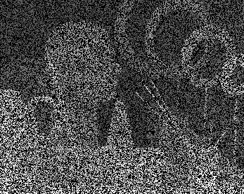
Figure 1: Left: Original disparity map. Middle: Corrupted disparity map with half pixels missing. Right: The inpainted result by low rank(LR) completion. We can see the inpainted map has much noise compared with original map.

However, statistics of depth image gradients show that the sparse gradient assumption is not accurate enough. The gradients can be described more properly as low rather than sparse. In another word, at many places in the depth image, gradients are not always 0 but rather very small (see Figure 4). This property has not been considered for image inpainting because it is not universal in general images. For depth images, statistics show the universality of this property. Hence we propose the low gradient regularization. We denote the low gradient regularization as $L_{0}^{\psi}$ gradient regularization. The notation comes from the corresponding non-convex TV^ψ norm [21]. Relation between them will be explained in the remainder part of this paper.

Unlike the $L_{0}$ norm which penalizes the non-zero elements equally (the norm is always 1 whether the element is 1 or 100), our proposed $L_{0}^{\psi}$ measure reduces the penalty for small elements. In depth images, our $L_{0}^{\psi}$ reduces the penalty for gradient 1 (all gradients are truncated into integer values) and thus allows for gradual depth changes.

Our main contributions are two-folds: First we propose the low gradient regularization $L_{0}^{\psi}$ which well describes the statistical property of the depth image gradients. Second we develop a solution to the $L_{0}^{\psi}$ gradient minimization problem based on [28]. We integrate our low gradient regularization with the low rank assumption into the LRL0^ψ regularization for depth image inpainting. In the experiments we compare our LRL0^ψ algorithm with two approaches, the low rank total variation (LRTV) [36] and the low rank L0 gradient (LRL0) approaches, which only enforce the sparse gradient constraint.

The remainder of the paper is organized as follows. Section II describes related work in image inpainting and the sparse gradient. Section III introduces the LRTV [36] and the LRL0 approaches which only consider the sparse gradient regularization. In section III we point out the defects of the sparse gradient regularization and then our main contribution, the low gradient regularization, is described in section IV. In section V we perform experiments on our dataset and display the experimental results. Finally We conclude our work in VI.

II Background

II-A Low Rank Matrix Completion

Completing a matrix with missing observations is an intriguing task in the machine learning and mathematics society [4], [7], [5], [24], [47]. Most work are based on the low rank assumption of the underlying data. The low rank matrix completion is one of effective approaches for image inpainting. Candes et al. [6] first introduce the matrix completion problem by approximating the rank with nuclear norm. Zhang et al. [46] propose the truncated nuclear norm regularization and achieve excellent results in image inpainting. Gu et al. [15] further present the weighted nuclear norm regularization and perform the image denoising task with outstanding results.

II-B Depth Inpainting

Depth image inpainting has been considered mostly under the situation of RGB-D inpainting or stereoscopic inpainting problems. Moreover, most depth inpainting approaches inpaint missing regions of specific kinds (e.g. occlusions, missing caused by sensor defects or holes caused by object-removal). Doria et al. [13] introduce a technique to fill holes in the LiDAR data sets. Wang et al. [43] present an algorithm for simultaneous color and depth inpainting. They take the stereo image pairs and the estimated disparity map as input and fill the holes cause by object removal. Lu et al. [26] cluster the RGB-D image patches into groups and employ the low rank matrix completion approach to enhance the depth images obtained from RGB-D sensors with the aid of corresponding color images. Zou et al. [48] consider inpainting RGB-D images by removing fence-like structures. Buyssens et al. [3] inpaint holes in the depth maps based on superpixel for virtual view synthesizing in RGB-D scenes. Herrera et al. [20] inpaint incomplete depth maps produced by 3D reconstruction methods under a second-order smoothness prior. As far as we know, almost all depth inpainting approaches refer to color images. They are either color-guided depth inpainting or simultaneous RGB-D inpainting. However, we consider inpainting only a single depth image.

II-C TV and $L_{0}$ Gradient Regularization

TV norm and its variations have been employed in image processing for quite a long time [9], [14]. Perrone et al. [30] propose a blind deconvolution algorithm based on the total variation minimization. Guo et al. [17] extend the total variation norm to tensors for visual data recovery. Li et al. [25] use the total variation in their robust noisy image completion algorithm.

Total variation refers to the integration of the norm of gradients on the whole image. When a function is applied to the norm of the gradients at each pixel before integral, the integration is called the total generalized variation. Hintermüller et al. [22] propose a nonconvex TV^q model for image restoration. They further propose a superlinearly solver for the general concave generalized TV model in [21]. Ranftl et al. [31] utilize the total generalized variation for optical flow estimation.

As mentioned above, the TV norm is a relaxation of the $L_{0}$ gradient. However, the TV norm also penalizes large gradient magnitudes. It may influence real image edges and boundaries [44]. Thus many algorithms directly solving $L_{0}$ gradient minimization have been proposed. Xu et al. [44] adopt a special alternating optimization strategy. They employ the method for image deblurring [45]. Their work is later applied for mesh denoising by He et al. [18]. Nguyen et al. [28] propose a fast $L_{0}$ gradient minimization approach based on a method named region fusion.

There are approaches that combine low rank regularization with the total variation minimization. Shi et al. [36] combine both the low rank and the total variation regularization into an LRTV algorithm for medical image super-resolution. Ji et al. [23] propose a tensor completion approach based on the total variation and the low-rank matrix completion. He et al. [19] employ the total variation regularization and the low-rank matrix factorization for hyperspectral image restoration.

III Low Rank Sparse Gradient Approach

In this section, we will review the LRTV [36] algorithm and introduce how it can be employed to inpaint depth images. Then the $L_{0}$ gradient is used to replace the TV regularization. We briefly review the algorithm developed by Nguyen et al. [28] for the $L_{0}$ gradient minimization. These are necessary for the explanation of our main contribution, the LRL0^ψ algorithm, which will be described in the next section.

Given a corrupted disparity map or depth image $\mathbf{D}$ and its inpainting mask $\mathbf{\Omega}$ (missing areas), we hope to recover the original image $\mathbf{U}$. The recovered image $\mathbf{U}$ should match the observations $\mathbf{U}|_{\Omega}=\mathbf{D}|_{\Omega}$. In conventional matrix completion image inpainting scheme, the low rank prior is added as a regularization [6], [15], [46] and the unknown image is recovered by solving

$$\arg\min_{\mathbf{U}}||\mathbf{U}-\mathbf{D}||^{2}_{\Omega}+\lambda\cdot\mathit{rank}(\mathbf{U})$$ (1)

$\lambda$ is a weight representing the importance of low rank. The above rank minimization problem is intractable due to the non-convexity and discontinuous nature of the rank function. Theoretical studies show that the nuclear norm is the tightest convex lower bound of the rank function of matrices [32]. Therefore, rank is usually approximated by the nuclear norm [6]. We employ the nuclear norm [6] as the low rank prior. As discussed in the introduction, we also add the sparse gradient regularization for depth recovery. Altogether we have the following formula

$$\arg\min_{\mathbf{U}}||\mathbf{U}-\mathbf{D}||^{2}_{\Omega}+\lambda_{r}\cdot||\mathbf{U}||_{*}+\lambda_{s}\cdot||\nabla\mathbf{U}||_{0}$$ (2)

Notice that the third term in equation 2 is the $L_{0}$ norm of gradient. Minimization corresponding to the $L_{0}$ norm is usually relaxed to $L_{1}$ norm and thus the $L_{0}$ gradient becomes total variation [36], [19], [23]. The $L_{0}$ norm is non-convex. The advantage of relaxing the $L_{0}$ gradient to total variation is that the problem becomes convex. We first employ the existed LRTV scheme as described in [36] for depth inpainting.

III-A Total Variation

The $L_{0}$ gradient norm is approximated by total variation and equation 2 now becomes

$$\arg\min_{\mathbf{U}}||\mathbf{U}-\mathbf{D}||^{2}_{\Omega}+\lambda_{r}\cdot||\mathbf{U}||_{*}+\lambda_{tv}\cdot TV(\mathbf{U})$$ (3)

This problem has almost the same form as the super-resolution problem in [36]. Following the solution in [36], we employ the ADMM alrgorithm [40] to solve the new equation

$$\begin{split}min_{\mathbf{U},\mathbf{M},\mathbf{Y}}||&\mathbf{U}-\mathbf{D}||^{2}_{\Omega}+\lambda_{r}||\mathbf{M}||_{*}+\lambda_{tv}TV(\mathbf{U})+\\ \frac{\rho}{2}&(||\mathbf{U}-\mathbf{M}+\mathbf{Y}||^{2}-||\mathbf{Y}||^{2})\end{split}$$ (4)

The minimization problem in equation 4 is broken into three sub-problems and the variables are iteratively updated.

The first subproblem needs to update $\mathbf{U}^{k+1}$ by minimizing part of equation 4 related with total variation.

$$\arg\min_{\mathbf{U}}||\mathbf{U}-\mathbf{D}||^{2}_{\Omega}+\lambda_{tv}TV(\mathbf{U})+\frac{\rho}{2}||\mathbf{U}-\mathbf{M}^{k}+\mathbf{Y}^{k}||^{2}$$ (5)

This subproblem is solved by Bregman iteration [27]. In the second subproblem $\mathbf{M}^{k+1}$ is updated by

$$\arg\min_{\mathbf{M}}||\mathbf{M}||_{*}+\frac{\rho}{2}||\mathbf{U}^{k+1}-\mathbf{M}+\mathbf{Y}^{k}||^{2}$$ (6)

After the update of $\mathbf{U}^{k+1}$ and $\mathbf{M}^{k+1}$, $\mathbf{Y}^{k+1}$ is updated by $\mathbf{Y}^{k+1}=\mathbf{Y}^{k}+(\mathbf{U}^{k+1}-\mathbf{M}^{k+1})$.

In our experiments, we initialize $\mathbf{U}$ as the coarse inpainting results obtained by the low rank matrix completion and $\mathbf{M}$ and $\mathbf{Y}$ are set to $\mathbf{0}$.

Figure 2: Top left: Groundtruth (GT). Top right: Corrupted with 50% missing entries. Lower left: Low rank inpainting [6]. Its PSNR = 27.7596. Lower right: LRTV result. Its PSNR = 28.1319. The LRTV approach obtains better results than only low rank. We also compute the TV norm for GT, low rank, and LRTV. They are 642186, 833767 and 622276 respectively. We can see the LRTV result has lower TV than GT. The $L_{0}$ norm of them are 63765, 117922 and 81644. The LRTV result has much higher $L_{0}$ norm than GT. In term of TV regularization, LRTV has achieved its optimal solution but in $L_{0}$ norm it is still far from optimal. The minimization of the TV norm does not necessarily mean the minimization of $L_{0}$ gradients.

The TV regularization improves the inpainting results compared with only low rank [6] (Figure 2). However, TV regularization has some drawbacks, it smoothes real depth edges [44]. We also observe that in depth inpainting results, the TV norm always becomes close and even lower than that of the groundtruth (see Figure 2). And even with a lower-than-groundtruth TV, the depth image remains noisy visually. We observe that even we optimize the results to have lower-than-groundtruth TV norm, the $L_{0}$ norm of gradients is still far above the groundtruth. Because the optimal solution under the TV norm regularization is not exactly optimal for the $L_{0}$ gradient , we decide to directly employ the $L_{0}$ gradient regularization.

In theory, the $L_{0}$ norm is the most suitable measure for sparsity. There are research on the gap between TV and $L_{0}$ (e.g. [29], [8]). There also have been work on directly solving $L_{0}$ gradient minimization problems [44], [28] by approximation strategies.

III-B $L_{0}$ Gradient

As mentioned above, the TV norm is widely used as the approximation of the $L_{0}$ norm of gradients for it enables fast and tractable solutions. However, the drawbacks of this approximation are also studied [44]. Therefore, a lot of approaches which directly and approximately minimize the $L_{0}$ gradient have been proposed [10], [44], [41], [28]. Among the approaches, Nguyen et al. [28] propose a region fusion method for $L_{0}$ gradient minimization. Their approach achieves rather good results while running the most efficiently compared with other $L_{0}$ gradient minimization algorithms [10], [44], [41].

We replace the TV norm in subproblem 2 (equation 5) with $L_{0}$ gradient

$$\arg\min_{\mathbf{U}}||\mathbf{U}-\mathbf{D}||^{2}_{\Omega}+\lambda_{l0}||\mathbf{\nabla U}||_{0}+\frac{\rho}{2}||\mathbf{U}-\mathbf{M}^{k}+\mathbf{Y}^{k}||^{2}$$ (7)

Following [28], we rewrite equation 7 as

$$\begin{split}\arg\min_{\mathbf{U}}\sum_{i=1}^{L}||U_{i}-D_{i}||^{2}_{\Omega}+&\frac{\rho}{2}||U_{i}-M^{k}_{i}+Y^{k}_{i}||^{2}\\ +&\frac{\lambda_{l0}}{2}\sum_{j\in N_{i}}||U_{i}-U_{j}||_{0}\end{split}$$ (8)

where $L$ is the length of the signal (the number of pixels in the image) and $N_{i}$ the neighboring set (four connected pixels) of the $i^{th}$ pixel.

The bold symbol like $\mathbf{U}$ indicates matrix and the normal symbol $U_{i}$, $M_{i}$, $D_{i}$ and $Y_{i}$ denote the values of $\mathbf{U}$, $\mathbf{M}$, $\mathbf{D}$ and $\mathbf{Y}$ at the $i$th pixel or the mean value in the $i$th region.

In [28] they propose an algorithm which loops though all neighboring regions (groups) $G_{i}$ and $G_{j}$. At first, all pixels are themselves groups. For region $G_{i}$, $D_{i}$, $M_{i}$ and $Y_{i}$ denote the mean value of $\mathbf{G}$, $\mathbf{D}$ and $\mathbf{Y}$ in the $i$th region $G_{i}$. We rewrite the pairwise region cost for our objective function as

$$\begin{split}f=\min_{U_{i},U_{j}}w_{i}||U_{i}-D_{i}||_{\Omega}^{2}+&w_{j}||U_{j}-D_{j}||_{\Omega}^{2}\\ +&\beta c_{i,j}||U_{i}-U_{j}||_{0}\\ +&\frac{\rho w_{i}}{2}||U_{i}-M^{k}_{i}+Y^{k}_{i}||^{2}\\ +&\frac{\rho w_{j}}{2}||U_{j}-M^{k}_{j}+Y^{k}_{j}||^{2}\end{split}$$ (9)

where $\beta$ is the auxiliary parameter ($0\leq\beta\leq\lambda$) [28].

The fusion criterion [28] derived from equation 9 which decides whether region $G_{i}$ and $G_{j}$ should be fused now becomes

$$\{U_{i},U_{j}\}=\begin{cases}\{A,A\}&\mathtt{if}\;f_{A}\leq f_{B}\\ \{B_{i},B_{j}\}&\mathtt{otherwise}\end{cases}$$ (10)

where $A=(\tilde{w}_{i}D_{i}+\tilde{w}_{j}D_{j}+\rho w_{i}M^{k}_{i}+\rho w_{j}M^{k}_{j}-\rho w_{i}Y^{k}_{i}-\rho w_{j}Y^{k}_{j})/(\tilde{w}_{i}+\tilde{w}_{j}+\rho w_{i}+\rho w_{j})$, $B_{i}=(2\tilde{w}_{i}D_{i}+\rho w_{i}(M^{k}_{i}-Y^{k}_{i}))/(2\tilde{w}_{i}+\rho w_{i})$, $B_{j}=(2\tilde{w}_{j}D_{j}+\rho w_{j}(M^{k}_{j}-Y^{k}_{j}))/(2\tilde{w}_{j}+\rho w_{j})$, $f_{A}$ is the value of equation 9 when $U_{i}=U_{j}=A$. $f_{B}$ is the value of equation 9 when $U_{i}=B_{i}$ and $U_{j}=B_{j}$. $w_{i}$ is the total number of pixels in region $i$ while $\tilde{w}_{i}$ only counts pixels in region $i$ that are meanwhile not in the missing region $\Omega$.

Then we modifty the region fusion minimization algorithm in [28] to solve the equation 8. In their original region fusion minimization, the two regions will remain untouched if the criterion equation 10 judges they should not be fused. In our settings, we will update them by $U_{i}=B_{i}$ and $U_{j}=B_{j}$.

The $L_{0}$ gradient regularization leads to better results in depth inpainting results in most cases. However, it does not always perform better than LRTV (see Figure 3). One of the reasons may be that the region fusion solution for $L_{0}$ gradient minimization is only an approximation. But beyond that, we have not fully utilized the features of the gradient maps. We compute the gradients of depth images and find out that the low $L_{0}$ norm is not accurate enough to characterize the property of depth image gradients (As shown in Figure 4). Besides 0, a non-ignorable part of pixels have gradient 1. In $L_{0}$ norm, all gradients larger than 0 are penalized equally. Based on the statistics of depth images, we hope to reduce the penalty for gradient 1 so that gradual depth change is allowed.

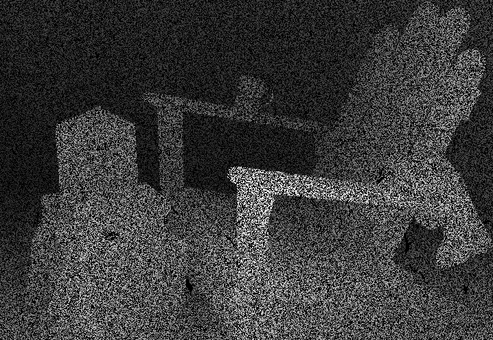
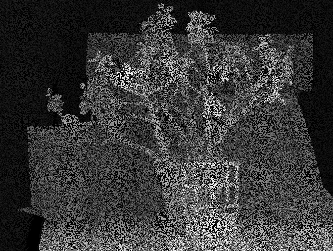
Figure 3: The first column are original depth images. The second column corresponds to the corrupted depth images. The third column displays the LRTV results. The last column shows our LRL0 results. For first row (Adirondack), the PSNR of LRTV and LRL0 are 28.1319 and 28.6198 respectively. For second row (Jadeplant), they are 22.8231 and 22.7730. We can see LRL0 achieves better inpainting results than LRTV on Adirondack but fails on Jadeplant.

IV Low Rank Low Gradient Approach

In this section, we will describe our main contribution, the LRL0^ψ algorithm. First we will point out our definition of the low gradient. Then we will describe our low rank low gradient regularization algorithm.

IV-A Integral Gradient

The magnitude of gradient is usually a real number. However, we will consider the gradients as integral values. We deal with depth images and disparity images with integral depth values. Thus the gradients on each direction take integral values. When doing statistics on the depth gradients, we truncate the magnitude of the gradients into integers. Denote the gradient as $(\nabla_{x},\nabla_{y})$, the truncation of the gradient magnitude is $\biggl{\lfloor}\sqrt{\nabla_{x}^{2}+\nabla_{y}^{2}}\biggr{\rfloor}$. Noting that the truncated value takes 0 only and if only the gradients on both directions are 0. The truncated gradient magnitude takes 1 if and only if the gradients are $(\pm 1,\pm 1)$, $(0,\pm 1)$ or $(\pm 1,0)$. In other words, for zero gradients, the real values and integral values are exactly the same. For gradient of value 1, it relates to 8 patterns $(\pm 1,\pm 1)$, $(0,\pm 1)$ or $(\pm 1,0)$. Our low gradient is defined on the integral gradients.

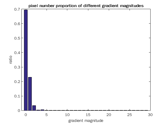
Figure 4: Gradient magnitude histogram of groundtruth disparity map of Middlebury Adirondack dataset. We can see most pixels have gradient magnitude 0 and a non-ignorable part have magnitude 1. This observation inspires us to employ low gradient regularization.

IV-B Low Gradient

As discussed in previous sections, the gradients of depth images cannot be simply depicted as sparse. The penalty of the small gradient value 1 should be reduced to allow for gradual depth changes (see Figure 4). There is a category of generalized TV^ψ norm [21] where the penalty of gradients are not increased linearly. Similar to the generalization of TV, we propose the $L_{0}^{\psi}$ norm so that the penalty for gradient 1 is reduced. Actually it is not a norm but rather a measure for the property of data because it does not satisfy the absolute homogeneity. Therefore we will call $L_{0}^{\psi}$ a measure. The $L_{0}^{\psi}$ measure is as follows:

$$||\mathbf{X}||_{L_{0}^{\psi}}=\alpha\#\{X=1\}+\#\{X>1\}$$ (11)

where $0<\alpha<1$ and $\#\{\cdot\}$ denotes the number of elements in the set.

We set $\alpha=0.75$ in all our experiments based on the statistics of groundtruth gradients.

Thus our low gradient leads to the following optimization problem:

$$\arg\min_{\mathbf{U}}||\mathbf{U}-\mathbf{D}||^{2}_{\Omega}+\lambda_{l0^{\psi}}||\mathbf{\nabla U}||_{l0^{\psi}}+\frac{\rho}{2}||\mathbf{U}-\mathbf{M}^{k}+\mathbf{Y}^{k}||^{2}$$ (12)

where $\lambda_{l0^{\psi}}$ is the weight of importance of the $L_{0}^{\psi}$ gradient term.

We extend the region fusion minimization in section III-B to solve $L_{0}^{\psi}$ gradient minimization problem.

In this case, the pairwise cost is as follows:

$$\begin{split}f=\min_{U_{i},U_{j}}w_{i}||U_{i}-&D_{i}||_{\Omega}^{2}+w_{j}||U_{j}-D_{j}||_{\Omega}^{2}\\ +&\beta c_{i,j}||U_{i}-U_{j}||_{L_{0}^{\psi}}\\ +&\frac{\rho w_{i}}{2}||U_{i}-M^{k}_{i}+Y^{k}_{i}||^{2}\\ +&\frac{\rho w_{j}}{2}||U_{j}-M^{k}_{j}+Y^{k}_{j}||^{2}\end{split}$$ (13)

The fusion criterion now contains three conditions. For groups $G_{i}$ and $G_{j}$,

• $U_{i}=U_{j}$. The optimal solution is $U_{i}=U_{j}=A$, where

  $$\begin{split}A&=\frac{A_{1}}{A_{2}}\\ A_{1}&=2(\tilde{w}_{i}D_{i}+\tilde{w}_{j}D_{j})+\rho w_{i}(M_{i}^{k}-Y_{i}^{k})\\ &+\rho w_{j}(M_{j}^{k}-Y^{k}_{j})\\ A_{2}&={2\tilde{w}_{i}+2\tilde{w}_{j}+\rho w_{i}+\rho w_{j}}\end{split}$$ (14)

  The function value of equation 13 under this condition is $f_{A}$.

• $|U_{i}-U_{j}|=1$, that is, $U_{j}=U_{i}\pm 1$. The optimal solution is $U_{i}=B$, $U_{j}=B\pm 1$, where

  $$\begin{split}B&=\frac{B_{1}}{A_{2}}\\ B_{1}&=2\tilde{w}_{i}D_{i}+2\tilde{w}_{j}(D_{j}\mp 1)\\ &+\rho w_{i}(M^{k}_{i}-Y^{k}_{i})\\ &+\rho w_{j}(M^{k}_{j}-Y^{k}_{j}\mp 1)\end{split}$$ (15)

  Denote the function value of equation 13 under this condition $f_{B}$.

• $|U_{i}-U_{j}|>1$. In this case $U_{i}=C_{i}$, $U_{j}=C_{j}$. $C_{i}=(2\tilde{w}_{i}D_{i}+\rho w_{i}(M^{k}_{i}-Y^{k}_{i}))/(2\tilde{w}_{i}+\rho w_{i})$, $C_{j}=(2\tilde{w}_{j}D_{j}+\rho w_{j}(M^{k}_{j}-Y^{k}_{j}))/(2\tilde{w}_{j}+\rho w_{j})$. We denote the function value as $f_{C}$.

  The fusion criterion now becomes:

  $$\{U_{i},U_{j}\}=\begin{cases}\{A,A\}&\mathtt{if}\;f_{A}\leq f_{B}\;\mathtt{and}\;f_{A}\leq f_{C}\\ \{B,B\pm 1\}&\mathtt{if}\;f_{B}<f_{A}\;\mathtt{and}\;f_{B}\leq f_{C}\\ \{C_{i},C_{j}\}&\mathtt{otherwise}\end{cases}$$ (16)

Based on this fusion criterion, we modify the region fusion iterations in [28] to solve the $L_{0}^{\psi}$ gradient minimization problem (see Algorithm 1). Our region fusion low gradient minimization algorithm is summarized in Algorithm 1. Notice that compared with the region fusion minimization algorithm for $L_{0}$ in [28], our algorithm has several differences. Similar to the modification in $L_{0}$ gradient minimization, when two regions are not to be fused by the fusion criterion, we update them to the optimal solutions $\{B,B\pm 1\}$ or $\{C_{i},C_{j}\}$ following equation 16.

Algorithm 1 Region Fusion Minimization for $L_{0}^{\psi}$

1:image $U$ with pixel number $N$, the level of sparseness $\lambda$, missing region $\Omega$, original missing image $D$, $Y$ and $M$

2:Initialize the regions as pixels themselves $G_{i}\leftarrow\{i\}$, $V_{i}\leftarrow C_{i}$, $w_{i}\leftarrow 1$

3:$\tilde{w}_{i}\leftarrow 0$ if $i\in\Omega$, otherwise $\tilde{w}_{i}\leftarrow 1$

4:Set $N_{i}$ as the four-connected neighborhood of $i$

5:Set $c_{i,j}=1$ if $j\in N_{i}$, otherwise $c_{i,j}=0$

6:$\beta\leftarrow 0$, $iter\leftarrow 0$, $P\leftarrow N$

7:repeat

8:     $i\leftarrow 1$

9:     while $i\leq P$ do

10:         for all $j\in N_{i}$ do

11:              Compute $f_{A},f_{B},f_{C}$ following Section IV

12:              if $f_{A}\leq f_{B}$ and $f_{A}\leq f_{C}$ then

13:                  $G_{i}\leftarrow G_{i}\cup G_{j}$

14:                  $V_{i}\leftarrow(w_{i}V_{i}+w_{j}V_{j})/(w_{i}+w_{j})$

15:                  $w_{i}\leftarrow w_{i}+w_{j}$

16:                  $\tilde{w}_{i}\leftarrow\tilde{w}_{i}+\tilde{w}_{j}$

17:                  Remove $j$ in $N_{i}$ and delete $c_{i,j}$

18:                  for all $k\in N_{j}\backslash\{i\}$ do

19:                       if $k\in N_{i}$ then

20:                           $c_{i,k}\leftarrow c_{i,k}+c_{j,k}$

21:                           $c_{k,i}\leftarrow c_{i,k}+c_{j,k}$

22:                       else

23:                           $N_{i}\leftarrow N_{i}\cup\{k\}$

24:                           $N_{k}\leftarrow N_{k}\cup\{i\}$

25:                           $c_{i,k}\leftarrow c_{j,k}$

26:                           $c_{k,i}\leftarrow c_{j,k}$

27:                       end if

28:                       Remove $j$ in $N_{k}$ and delete $c_{k,j}$

29:                  end for

30:                  Delete $G_{j}$,$N_{j}$,$w_{j}$

31:              else if $f_{B}<f_{A}$ and $f_{B}\leq f_{C}$ then

32:                  if $U_{i}>U_{j}$ then

33:                       $V_{i}\leftarrow B$, $V_{j}\leftarrow B-1$

34:                  else

35:                       $V_{i}\leftarrow B$, $V_{j}\leftarrow B+1$

36:                  end if

37:              end if

38:              $P\leftarrow P-1$, $i\leftarrow i+1$

39:         end for

40:     end while

41:     $iter\leftarrow iter+1$

42:     $\beta\leftarrow(iter/K)\lambda$

43:until $\beta>\lambda$

44:for $i=1\to P$ do

45:     for all $j\in G_{i}$ do

46:         $S_{j}\leftarrow V_{i}$

47:     end for

48:end for

49:filtered Image $S$

V Experiments and Results

Figure 5: The left is an example of the random missing pattern. The right is an example of the textual missing mask.

V-A Dataset

For there is no public dataset that aims at inpainting depth images, we make a dataset for evaluating depth inpainting approaches. We convert the groundtruth disparity maps from Middlebury stereo dataset [35] to grayscale depth images. The groundtruth depth maps are from 14 images including Adirondack, Jadeplant, Motorcycle, Piano, Playtable, Playroom, Recycle, Shelves, Teddy, Pipes, Vintage, MotorcycleE, PianoL and PlaytableP. The unknown values of the groundtruth disparity maps are converted to 0s in depth images. To create damaged images, we generate several masks including random missing masks (see Figure 5) and textual masks (see Figure 5). The masks are provided in our dataset.

In addition to the depth images and masks, we also provide our results which will be displayed in this section together with our codes for all the algorithms concerned in this paper. Our codes also enable generations of new random masks. New depth images can also be processed by our codes to produce inpainted results. Our dataset can be accessed via http://www.cad.zju.edu.cn/home/dengcai/Data/depthinpaint/DepthInpaintData.html. Our code can be accessed via https://github.com/xuehy/depthInpainting.

V-B Experiments

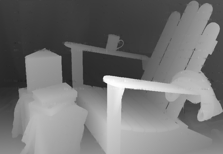
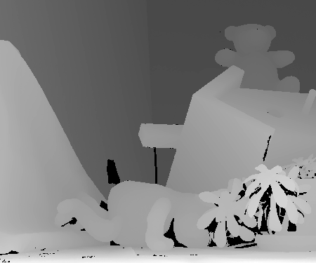
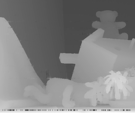
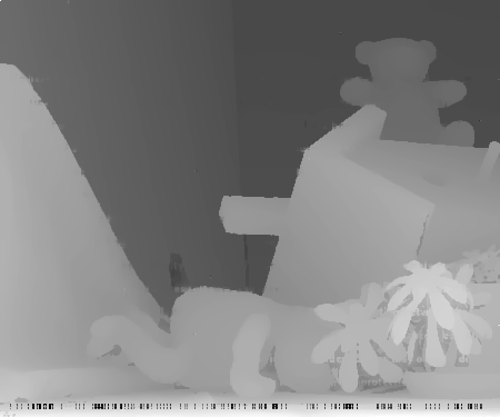
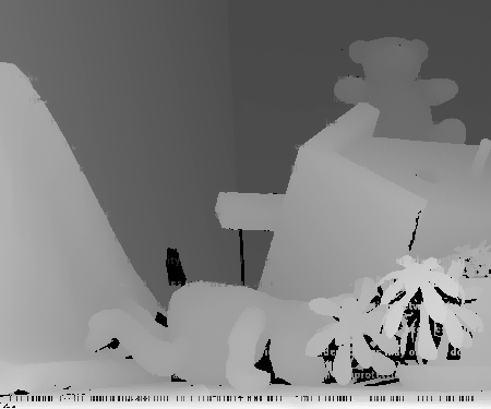
Figure 6: In this figure we show the results of Adirondack and Teddy with textual mask. For every image, the first row shows the original depth image, the damaged image and the low rank result (from left to right). The second row displays the result of LRTV, LRL0 and LRL0^ψ (from left to right). The PSNR of Adirondack are 28.2444(Low rank), 28.3886(LRTV), 28.9374(LRL0) and 29.2523(LRL0^ψ). The PSNR of Teddy are 16.3590, 16.9535, 17.0616 and 17.1101.

We first inpaint the depth images with the nuclear norm regularization matrix completion approach. Then we apply the LRTV approach which is first used by Shi et al. [36] for medical image super-resolution. From the inpainted results, we can see LRTV reduces noise caused by the low rank completion. Later on, we employ the LRL0 algorithm. As we can see, although LRL0 outperforms LRTV in most cases, it fails on some depth images. As discussed in section III-B, we propose the low gradient measure and the corresponding LRL0^ψ algorithm based on the statistics of depth gradient maps. In the end we inpaint the images with LRL0^ψ. We evaluate the inpainted results using PSNR and the PSNR is computed only on the missing area of the depth images.

V-C Parameters and Setup

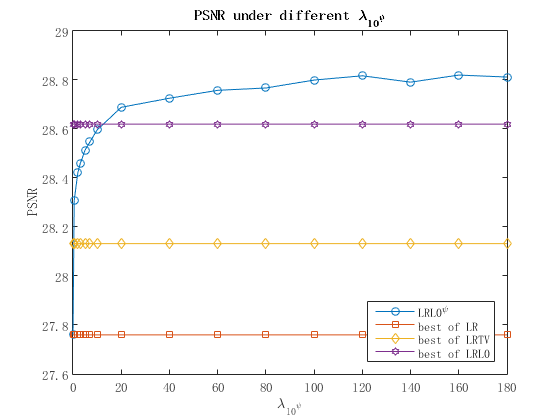
Figure 7: For the LRL0^ψ algorithm we search for the best value of $\lambda_{l0^{\psi}}$ for the image Adirondack. The $\lambda_{l0^{\psi}}$ with highest PSNR is reported as the result. This figure shows the results of LRL0^ψ under different parameters. The best results of the other methods are reported here. We can see our LRL0^ψ achieves better results than the other approaches when the parameter gets large enough.

The experiments are performed on a PC of Intel i7 3.5GHz CPU with 16GB memory. Our parameter settings are listed as follows. For all algorithms, we set the weight for the low rank term $\lambda_{r}=10$.

• For LRTV: we set the weight for TV term to $\lambda_{tv}=40$.

• For LRL0: we set the weight as $\lambda_{l0}=30$.

• For LRL0^ψ: we set the weight as $\lambda_{l0^{\psi}}=100$.

For all algorithms, the iterations are stopped when the the number of iterations exceeds 30 or the relative error of solutions is below $1\times 10^{-3}$.

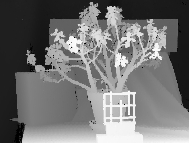
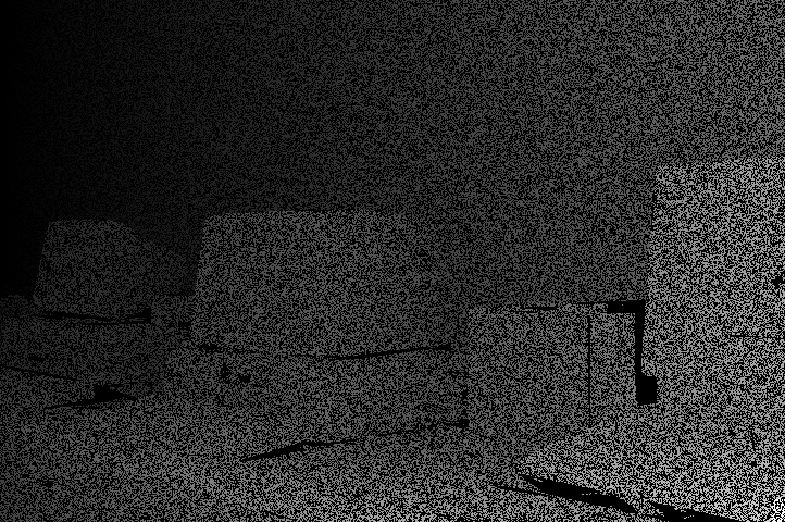
Figure 8: In this figure we show the results of three images: Adirondack, Jadeplant and Vintage. For every image, the first row shows the original depth image, the damaged image and the low rank result (from left to right). The second row displays the result of LRTV, LRL0 and LRL0^ψ (from left to right). The PSNR of Adirondack are 27.7596(Low rank), 28.1319(LRTV), 28.6198(LRL0) and 28.8292(LRL0^ψ). The PSNR of Jadeplant are 21.9843, 22.8231, 22.7730 and 22.8725. The PSNR of Vintage are 22.7924, 23.2368, 24.0400 and 24.2091.

V-D Results and Analysis

Mask type	Adiron	Jadepl	Motor	Piano
Method	rand	rand	rand	rand
LR	27.7596	21.9843	22.0838	18.2673
LRTV	28.1319	22.8231	22.7546	18.5161
LRL0	28.6198	22.7730	22.9303	19.5263
LRL0ψ	28.8292	22.8725	23.1480	19.6801
Mask type	Playt	Playrm	Recyc	Shelvs
Method	rand	rand	rand	rand
LR	22.8384	17.7783	23.5558	14.9259
LRTV	23.2150	18.0073	23.9033	15.3300
LRL0	24.3513	18.6153	24.7019	16.1661
LRL0ψ	24.4886	18.7681	24.8112	16.2910
Mask type	Teddy	Pipes	Vintge	MotorE
Method	rand	rand	rand	rand
LR	19.5329	22.1899	22.7924	22.3541
LRTV	20.0866	22.9039	23.2368	23.2859
LRL0	20.7570	23.4278	24.0400	23.1577
LRL0ψ	20.8839	23.6760	24.2091	23.3850
Mask type	PianoL	PlaytP	adi	ted
Method	rand	rand	text	text
LR	19.8488	23.9959	28.2444	16.359
LRTV	20.1330	23.2150	28.3886	16.9535
LRL0	21.3011	25.6337	28.9347	17.0616
LRL0ψ	21.4553	25.8008	29.2523	17.1101

TABLE I: PSNR of results from different inpainting methods on our dataset. The mask type indicates what kind of mask is applied to make the depth image with missing areas. rand indicates random missing and text indicates textual masks. Noting that our proposed LRL0 approach performs generally better than LRTV and achieves relatively close results to LRL0^ψ. However, LRL0 gets worse-than-LRTV results on MotorE and Jadeplant. Our proposed LRL0^ψ approach always achieves the best results in PSNR.

Some of the experimental results are shown in Figure 6 and Figure 8. The PSNR of the results of the whole dataset are shown in Table I. The low rank results have obvious noise (see Figure 6 and 8). Noting that the LRL0 approach performs generally better than LRTV and achieves relatively close results to LRL0^ψ. However, LRL0 gets worse-than-LRTV results on MotorE and Jadepl. For high resolution results, please refer to our published dataset. Our proposed LRL0^ψ approach always achieves the best results in PSNR because it allows for gradual pixel value variation which is common in depth images.

V-E Parameter Analysis

We tune the parameter $\lambda_{l0^{\psi}}$ to see the effect of the weight of the low gradient regularization term. The resultant PSNR curve is shown in Figure 7. When $\lambda_{l0^{\psi}}=0$, the LRL0^ψ algorithm degenerates to the LR algorithm. As $\lambda_{l0^{\psi}}$ increases, the low gradient term gets more important and the inpainting result improves over the LR algorithm. When $\lambda_{l0^{\psi}}$ gets large enough(exceeds 80), the resultant PSNR gets stable. The LRL0^ψ algorithm outperforms the other approaches when the weight $\lambda_{l0^{\psi}}$ for the low gradient term gets large enough.

VI Conclusions

We consider the problem of inpainting depth images. The popular image inpainting technique low rank matrix completion always leads to noisy depth inpainting results. Based on the gradient statistics of depth images, we propose the low gradient regularization and combine it with the low rank prior into the LRL0^ψ approach. Then we extend the region fusion approach in [28] for our $L_{0}^{\psi}$ gradient minimization problem. We compare our approach with the only low rank regularization and two other approaches, the LRTV and the LRL0 approaches, which only enforce sparse gradient regularization. Experiments show that our proposed methods outperform the only low rank method. Our proposed LRL0^ψ approach also outperforms the LRTV and LRL0 approaches for it better utilizes the gradient property.

Hongyang Xue Hongyang Xue received the B.E. degree in Computer Science and Technology from Zhejiang University, China, in 2014. He is currently a Ph.D. candidate in Computer Science at Zhejiang University. His research include machine learning, computer vision and data mining.

Shengming Zhang Shengming Zhang is an intern in the State Key Laboratory of CAD&CG, Undergraduate of Computer Science at Zhejiang University, China. He will receive the Bachelor’s degree in Computer Science from Zhejiang University in 2017. His research interests include computer vision, computer graphics and machine learning.

Deng Cai Deng Cai is a Professor in the State Key Laboratory of CAD&CG, College of Computer Science at Zhejiang University, China. He received the Ph.D. degree in Computer Science from the University of Illinois at Urbana Champaign in 2009. His research interests include machine learning, data mining and information retrieval.

References

- [1] M. Bertalmio, G. Sapiro, V. Caselles, and C. Ballester. Image inpainting. In Proceedings of the 27th annual conference on Computer graphics and interactive techniques, pages 417–424. ACM Press/Addison-Wesley Publishing Co., 2000.
- [2] A. Buades, B. Coll, and J.-M. Morel. Image denoising methods. a new nonlocal principle. SIAM review, 52(1):113–147, 2010.
- [3] P. Buyssens, M. Daisy, D. Tschumperlé, and O. Lézoray. Superpixel-based depth map inpainting for rgb-d view synthesis. In Image Processing (ICIP), 2015 IEEE International Conference on, pages 4332–4336. IEEE, 2015.
- [4] J.-F. Cai, E. J. Candès, and Z. Shen. A singular value thresholding algorithm for matrix completion. SIAM Journal on Optimization, 20(4):1956–1982, 2010.
- [5] E. J. Candes and Y. Plan. Matrix completion with noise. Proceedings of the IEEE, 98(6):925–936, 2010.
- [6] E. J. Candès and B. Recht. Exact matrix completion via convex optimization. Foundations of Computational mathematics, 9(6):717–772, 2009.
- [7] E. J. Candès and T. Tao. The power of convex relaxation: Near-optimal matrix completion. Information Theory, IEEE Transactions on, 56(5):2053–2080, 2010.
- [8] E. J. Candes, M. B. Wakin, and S. P. Boyd. Enhancing sparsity by reweighted ℓ 1 minimization. Journal of Fourier analysis and applications, 14(5-6):877–905, 2008.
- [9] T. Chan, S. Esedoglu, F. Park, and A. Yip. Recent developments in total variation image restoration. Mathematical Models of Computer Vision, 17:2, 2005.
- [10] X. Cheng, M. Zeng, and X. Liu. Feature-preserving filtering with l 0 gradient minimization. Computers & Graphics, 38:150–157, 2014.
- [11] A. Criminisi, P. Pérez, and K. Toyama. Region filling and object removal by exemplar-based image inpainting. Image Processing, IEEE Transactions on, 13(9):1200–1212, 2004.
- [12] S. Dai and Y. Wu. Removing partial blur in a single image. In Computer Vision and Pattern Recognition, 2009. CVPR 2009. IEEE Conference on, pages 2544–2551. IEEE, 2009.
- [13] D. Doria and R. J. Radke. Filling large holes in lidar data by inpainting depth gradients. In Computer Vision and Pattern Recognition Workshops (CVPRW), 2012 IEEE Computer Society Conference on, pages 65–72. IEEE, 2012.
- [14] B. Goldluecke and D. Cremers. An approach to vectorial total variation based on geometric measure theory. In Computer Vision and Pattern Recognition (CVPR), 2010 IEEE Conference on, pages 327–333. IEEE, 2010.
- [15] S. Gu, L. Zhang, W. Zuo, and X. Feng. Weighted nuclear norm minimization with application to image denoising. In Proceedings of the IEEE Conference on Computer Vision and Pattern Recognition, pages 2862–2869, 2014.
- [16] C. Guillemot and O. Le Meur. Image inpainting: Overview and recent advances. Signal Processing Magazine, IEEE, 31(1):127–144, 2014.
- [17] X. Guo and Y. Ma. Generalized tensor total variation minimization for visual data recovery? In Computer Vision and Pattern Recognition (CVPR), 2015 IEEE Conference on, pages 3603–3611. IEEE, 2015.
- [18] L. He and S. Schaefer. Mesh denoising via l 0 minimization. ACM Transactions on Graphics (TOG), 32(4):64, 2013.
- [19] W. He, H. Zhang, L. Zhang, and H. Shen. Total-variation-regularized low-rank matrix factorization for hyperspectral image restoration. Geoscience and Remote Sensing, IEEE Transactions on, 54(1):178–188, 2016.
- [20] D. Herrera, J. Kannala, J. Heikkilä, et al. Depth map inpainting under a second-order smoothness prior. In Image Analysis, pages 555–566. Springer, 2013.
- [21] M. Hintermüller and T. Wu. A superlinearly convergent r-regularized newton scheme for variational models with concave sparsity-promoting priors. Computational Optimization and Applications, 57(1):1–25, 2014.
- [22] M. Hintermüller and T. Wu. Nonconvex tv ^q-models in image restoration: Analysis and a trust-region regularization–based superlinearly convergent solver. SIAM Journal on Imaging Sciences, 6(3):1385–1415, 2013.
- [23] T.-Y. Ji, T.-Z. Huang, X.-L. Zhao, T.-H. Ma, and G. Liu. Tensor completion using total variation and low-rank matrix factorization. Information Sciences, 326:243–257, 2016.
- [24] R. H. Keshavan, S. Oh, and A. Montanari. Matrix completion from a few entries. In Information Theory, 2009. ISIT 2009. IEEE International Symposium on, pages 324–328. IEEE, 2009.
- [25] W. Li, L. Zhao, D. Xu, and D. Lu. A non-local method for robust noisy image completion. In Computer Vision–ECCV 2014, pages 61–74. Springer, 2014.
- [26] S. Lu, X. Ren, and F. Liu. Depth enhancement via low-rank matrix completion. In The IEEE Conference on Computer Vision and Pattern Recognition (CVPR), June 2014.
- [27] A. Marquina and S. J. Osher. Image super-resolution by tv-regularization and bregman iteration. Journal of Scientific Computing, 37(3):367–382, 2008.
- [28] R. M. Nguyen and M. S. Brown. Fast and effective l0 gradient minimization by region fusion. In Proceedings of the IEEE International Conference on Computer Vision, pages 208–216, 2015.
- [29] X. Pang, S. Zhang, J. Gu, L. Li, B. Liu, and H. Wang. Improved l 0 gradient minimization with l 1 fidelity for image smoothing. PloS one, 10(9):e0138682, 2015.
- [30] D. Perrone and P. Favaro. Total variation blind deconvolution: The devil is in the details. In Computer Vision and Pattern Recognition (CVPR), 2014 IEEE Conference on, pages 2909–2916. IEEE, 2014.
- [31] R. Ranftl, K. Bredies, and T. Pock. Non-local total generalized variation for optical flow estimation. In Computer Vision–ECCV 2014, pages 439–454. Springer, 2014.
- [32] B. Recht, M. Fazel, and P. A. Parrilo. Guaranteed minimum-rank solutions of linear matrix equations via nuclear norm minimization. SIAM review, 52(3):471–501, 2010.
- [33] X. Ren, L. Bo, and D. Fox. Rgb-(d) scene labeling: Features and algorithms. In Computer Vision and Pattern Recognition (CVPR), 2012 IEEE Conference on, pages 2759–2766. IEEE, 2012.
- [34] M. Rohrbach, S. Amin, M. Andriluka, and B. Schiele. A database for fine grained activity detection of cooking activities. In Computer Vision and Pattern Recognition (CVPR), 2012 IEEE Conference on, pages 1194–1201. IEEE, 2012.
- [35] D. Scharstein and R. Szeliski. A taxonomy and evaluation of dense two-frame stereo correspondence algorithms. International journal of computer vision, 47(1-3):7–42, 2002.
- [36] F. Shi, J. Cheng, L. Wang, P.-T. Yap, and D. Shen. Low-rank total variation for image super-resolution. In Medical Image Computing and Computer-Assisted Intervention–MICCAI 2013, pages 155–162. Springer, 2013.
- [37] J. Shi, X. Ren, G. Dai, J. Wang, and Z. Zhang. A non-convex relaxation approach to sparse dictionary learning. In Computer Vision and Pattern Recognition (CVPR), 2011 IEEE Conference on, pages 1809–1816. IEEE, 2011.
- [38] N. Silberman, D. Hoiem, P. Kohli, and R. Fergus. Indoor segmentation and support inference from rgbd images. In Computer Vision–ECCV 2012, pages 746–760. Springer, 2012.
- [39] S. Song and J. Xiao. Sliding shapes for 3d object detection in depth images. In Computer Vision–ECCV 2014, pages 634–651. Springer, 2014.
- [40] B. Stephen, P. Neal, C. Eric, P. Borja, and E. Jonathan. Distributed optimization and statistical learning via the alternating direction method of multipliers. Found. Trends Mach. Learn, 3(1):1–122, 2011.
- [41] M. Storath, A. Weinmann, and L. Demaret. Jump-sparse and sparse recovery using potts functionals. Signal Processing, IEEE Transactions on, 62(14):3654–3666, 2014.
- [42] Y. Tang, R. Salakhutdinov, and G. Hinton. Robust boltzmann machines for recognition and denoising. In Computer Vision and Pattern Recognition (CVPR), 2012 IEEE Conference on, pages 2264–2271. IEEE, 2012.
- [43] L. Wang, H. Jin, R. Yang, and M. Gong. Stereoscopic inpainting: Joint color and depth completion from stereo images. In Computer Vision and Pattern Recognition, 2008. CVPR 2008. IEEE Conference on, pages 1–8. IEEE, 2008.
- [44] L. Xu, C. Lu, Y. Xu, and J. Jia. Image smoothing via l 0 gradient minimization. In ACM Transactions on Graphics (TOG), volume 30, page 174. ACM, 2011.
- [45] L. Xu, S. Zheng, and J. Jia. Unnatural l0 sparse representation for natural image deblurring. In Proceedings of the IEEE Conference on Computer Vision and Pattern Recognition, pages 1107–1114, 2013.
- [46] D. Zhang, Y. Hu, J. Ye, X. Li, and X. He. Matrix completion by truncated nuclear norm regularization. In Computer Vision and Pattern Recognition (CVPR), 2012 IEEE Conference on, pages 2192–2199. IEEE, 2012.
- [47] Y. Zheng, G. Liu, S. Sugimoto, S. Yan, and M. Okutomi. Practical low-rank matrix approximation under robust l 1-norm. In Computer Vision and Pattern Recognition (CVPR), 2012 IEEE Conference on, pages 1410–1417. IEEE, 2012.
- [48] Q. Zou, Y. Cao, Q. Li, Q. Mao, and S. Wang. Automatic inpainting by removing fence-like structures in rgbd images. Machine Vision and Applications, 25(7):1841–1858, 2014.